
Statistical Modeling Approaches for PM10 Prediction in Urban Areas; A Review of 21st-Century Studies

Abstract
:1. Introduction
2. Search Strategy and Study Selection
3. PM10 Predictors in Statistical Models
4. Temporal Prediction (Forecasting) of PM10 in Urban Areas
4.1. Multi-Variate Linear Regression (MLR)

| PM10 Parameter | Method ** | Forecasting Time-Scale | Case Study | Country | Inputs * | Results *** | Time Series | Ref. |
|---|---|---|---|---|---|---|---|---|
| Monthly | MLP | -**** | One station in Janipur | India | TV, WS, WD, RH, Ta | RMSE = 7.9, R = 0.7 | 1993–1998 | [64] |
| Daily | MLP | Mean and maximum one day ahead | One station in Lawer Fraster Valley | Canada | PM10, PM2.5, NO, CO, NO2, MVs and TVs | Mean PM10: R = 0.65 | 1995–1999 | [65] |
| Maximum PM10: R = 0.66 | ||||||||
| Daily | MLR | Mean and maximum one day ahead | One station in Lawer Fraster Valley | Canada | PM10, PM2.5, NO, CO, NO2, MVs and TVs | Mean PM10: R = 0.7 | 1995–1999 | [65] |
| Maximum PM10: R = 0.69 | ||||||||
| Daily | MLP | One-day | One station in Athens | Greece | Model 1: WS, DT, DOW, RH, WDI Model2: Lagged PM10, WS, DT, DOW, RH, WDI | Model 1: MAE = 16.0, RMSE = 21.2, R2 = 0.47 | 1 June 1999–31 May 2001 | [66] |
| Model 2: MAE = 12.6, RMSE = 16.9, R2 = 0.65 | ||||||||
| Daily | MLR | One-day | One station in Athens | Greece | Model 1: WS, DT, DOW, RH, WDI Model 2: Lagged PM10, WS, DT, DOW, RH, WDI | Model 1: MAE = 18.0, RMSE = 23.4, R2 = 0.34 | 1 June 1999–31 May 2001 | [66] |
| Model 2: MAE = 14.7, RMSE = 18.37, R2 = 0.6 | ||||||||
| Hourly | MLR | One hour | 2 stations in Helsinki | Finland | TVs (e.g., CDAY and HOD), MVs, and traffic flow variables | R = 0.2–0.24 | 1996–1999 | [35] |
| Hourly | MLP | One hour | 2 stations in Helsinki | Finland | TVs (e.g., CDAY and HOD), MVs, and traffic flow variables | R = 0.31–0.42 | 1996–1999 | [35] |
| Daily | RBF | 3 days ahead | One station in Hong Kong | Hong Kong | PM10, SO2, NO, CO, NO2, NOx, WA; WD; SR; Ta | MAE = 12.5, RMSE = 16.3 | 2000 | [67] |
| Daily | RBF | 3 days ahead | One station in Hong Kong | Hong Kong | 6 PCs of combination of PM10, SO2, NO, CO, NO2, NOx, WS, WD, SR and Ta | MAE = 16.4, RMSE = 21.4 | 2000 | [67] |
| Daily | MLP | One day | One station in Milan | Italy | PM10, SO2, Ta, P | R = 0.88 MAE = 8.59 | 1999–2002 | [68] |
| Daily | PNN | One day | One station in Milan | Italy | PM10, SO2, Ta, P | R = 0.89 MAE = 8.55 | 1999–2002 | [68] |
| Daily | LL | One day | One station in Milan | Italy | PM10, SO2, Ta, P | R = 0.90 MAE= 8.25 | 1999–2002 | [68] |
| Daily | MLP | One-day ahead | 10 Urban stations in 10 cities | Belgium | First 9-hourly PM10 in current day and daily forecasts of BLH, WS, Ta, CC, WD, DOW for one-day ahead | RMSE: about 12–24 R: about 0.67–0.81 | 1997–2001 | [5] |
| Hourly | MLP | 24 h ahead | 4 stations in Athens | Greece | PM10 (t−24), PM10 (t−25), PM10 (t−26), WS, Ta, RH, SR, WD, DOW, SEA, SDAY, CDAY | R = 0.7–0.82 | 2001–2002 | [58] |
| Hourly | MLP | 24 h ahead | 4 stations in Athens | Greece | PM10 (t−24), PM10 (t−25), PM10 (t−26) | R = 0.43–0.54 | 2001–2002 | [58] |
| Hourly | MLP | 24 h ahead | 4 stations in Athens | Greece | Different set of variables were selected for the 4 stations | R = 0.65–0.83 | 2001–2002 | [58] |
| Hourly | MLR | 24 h ahead | 4 stations in Athens | Greece | 10 variables were selected | R = 0.55–0.59 | 2001-2002 | [58] |
| Daily | MLP and MLR | Maximum one-day ahead | 5 stations in Santiago | Chile | Some hourly PM10 in day t−1, and some meteorological observations and forecasts | Contingency table | 2001–2004 | [69] |
| Daily maximum | ELMAN | Two-days ahead | Five stations in Palermo | Italy | Hourly WS, WD, Ta, P | RMSE = 4.53–6.47 R = 0.93–0.97 MAE = 2.77–5.58 | 1 January 2003–31 December 2004 | [2] |
| Daily | MLP | One day ahead | One station in Volos | Greece | PM10 (t−1), DOW; MOY, Tmax-Tmin, WS | R = 0.78 RMSE = 11.4 | 2001–2003 | [56] |
| Daily | MLR | One day ahead | One station in Volos | Greece | PM10 (t−1), DOW; MOY, Tmax-Tmin, WS | R = 0.74 RMSE = 11.2 | 2001–2003 | [56] |
| Daily | MLR | Daily | One station in Graz | Austria | Meteorological forecasts and TVs; PM10 (t−1) and Ta (t−1) | R2 = 0.69 | 2001–2007 | [32] |
| Daily | MLR | Daily | One station in Klagenfurt | Austria | Meteorological forecasts and TVs; PM10 (t−1) and Ta (t−1) | R2 = 0.7 | 2003–2005 | [32] |
| Daily | MLR | Daily | One station in Bolzano | Italy | Meteorological forecasts and TVs; PM10 (t−1) and Ta (t−1) | R2 = 0.55 | 2001–2006 | [32] |
| Hourly | MLP | Hourly | Three traffic sites in Guangzhou | China | 7 MVs: WS, Ta, P, WD, Rf, SR, RH 3 background parameters: PM10 (t−1), PM10 (t−2), PM10 (t−3) 2 TVs: DOW, HOD; TrV; 3 geographical parameters: DRC, SD, SAR | One hour ahead: MAPE = 12.9%; MAE = 15.5; RMSE = 20.1 R = 0.961 Some hours ahead: MAPE = 22.4%; MAE = 35; RMSE = 57.5; R = 0.912 | 2007 | [70] |
| Hourly | MLR | Hourly | Three traffic sites in Guangzhou | China | WS, SR, RH, PM10 (t−1), PM10 (t−2), PM10 (t−3) TrV DRC | One hour ahead: R = 0.971 Some hours ahead: R= 0.894 | 2007 | [70] |
| Hourly | MLP | One hour ahead | One station in Zagreb | Croatia | PM10(t−1), MVs, TVs | R = 0.72 MAE = 9.34 RMSE = 13.3 | 2004–2005 | [36] |
| Hourly | MLP | One hour ahead | 4 stations in four urban areas | Cyprus | PM10 (t−24), PM10 (t−25), PM10 (t−26), MVs, TVs | R2 = 0.65–0.76 RMSE = 13–32 | 2006–2008 | [33] |
| Hourly | RBF | One hour ahead | 4 stations in four urban areas | Cyprus | PM10 (t−24), PM10 (t−25), PM10 (t−26), MVs, TVs | R2 = 0.37–0.43 RMSE = 19.5–35 | 2006–2008 | [33] |
| Hourly | PCRA | One hour ahead | 4 stations in four urban areas | Cyprus | PM10 (t−24), PM10 (t−25), PM10 (t−26), MVs, TVs | R2 = 0.33–0.38 RMSE = 17.8–26.2 | 2006–2008 | [33] |
| Hourly | MLP | 24 h ahead | One station, Phoenix | Arizona | PM10, meteorological data | R2 = 0.38 | 2005 | [51] |
| Daily maximum | MLP | One day ahead | 8 stations in Santiago | Chile | PM10, meteorological information | MPAE = 14%–27% | 2006–2011 | [71] |
| Daily | MLP | Maximum one day ahead | 9 stations in Tehran | Iran | PM10, NO, CO, MVs, TVs | R = 0.05–0.72 | 2001–2009 | [72] |
| Hourly | MLP | 2 h ahead | One station in London | UK | PM10 (t−2), WS (t−2), WD (t-2) | R2 = 0.98 | January 2009 | [73] |
| Daily | MLP | - | 36 stations in Changsha | China | MVs | R2 = 0.89 | April 2013–April 2014 | [74] |
| Daily | MLR | - | 36 stations in Changsha | China | MVs | R2 = 0.47 | April 2013–April 2014 | [74] |
4.2. Artificial Neural Networks
| Evaluation Statistics | Abbreviation | Model 1: MLR | Model 1: ANN | Model 2: MLR | Model 2: ANN |
|---|---|---|---|---|---|
| Probability of Detection or Fraction of Correctly Forecasted exceedances | 0.91 | 0.93 | 0.93 | 0.93 | |
| False Alarm Rate | 0.3 | 0.2 | 0.17 | 0.13 | |
| Threat Score or Success Index | 0.65 | 0.75 | 0.78 | 0.82 |
4.3. Other Techniques
| PM10 Parameter | Method ** | Forecasting Time-Scale | Case Study | Country | Inputs * | Results *** | Time Series | Source |
|---|---|---|---|---|---|---|---|---|
| Hourly | GAM | -**** | Four stations in Oslo | Norway | TVs, MVs, and traffic variables | R2 = 0.48–0.72 | November 2001–May 2003 | [76] |
| Daily | MLR | One-day | One station in Delhi | India | WS, RH, SR, Ta | R2 = 0.58 | 2000–2002 | [37] |
| Daily | ARIMA | One-day | One station in Delhi | India | Daily PM10 | R2 = 0.73 | 2000–2002 | [37] |
| Daily | Hybrid MLR and ARIMA | One-day | One station in Delhi | India | WS, RH, SR, Ta, Daily PM10 | R2 = 0.77 | 2000–2002 | [37] |
| Daily | MLR | One-day | One station in Hong Kong | Hong Kong | WS, RH, SR, Ta | R2 = 0.54 | 2000–2001 | [37] |
| Daily | ARIMA | One-day | One station in Hong Kong | Hong Kong | Daily PM10 | R2 = 0.8 | 2000–2001 | [37] |
| Daily | Hybrid MLR and ARIMA | One-day | One station in Hong Kong | Hong Kong | WS, RH, SR, Ta, Daily PM10 | R2 = 0.84 | 2000–2001 | [37] |
| Daily | MLR | Daily | One station in Thessaloniki | Greece | MVs | R = 0.297 | 1994–2000 | [52] |
| MAE = 49 | ||||||||
| PCR | R = 0.235 | |||||||
| MAE = 34 | ||||||||
| CART | R = 0.386 | |||||||
| MAE = 28 | ||||||||
| MLP | R = 0.249 | |||||||
| MAE = 25 | ||||||||
| Daily | MLP | One-day | One station in Temuco | Chile | WS, Tmin, Tmax, hourly maximum PM10 | RMSE = 28.6, R2 = 0.78 | 2000–2006 | [34] |
| Daily | MLR | One-day | One station in Temuco | Chile | WS, Tmin, Tmax, hourly maximum PM10 | RMSE = 28.4, R2 = 0.78 | 2000–2006 | [34] |
| Daily | ARMAX | One-day | One station in Temuco | Chile | WS, Tmin, Tmax, hourly maximum PM10 | RMSE = 28.5, R2 = 0.77 | 2000–2006 | [34] |
| Daily | Hybrid ARMAX-ANN | One-day | One station in Temuco | Chile | WS, Tmin, Tmax, hourly maximum PM10 | RMSE = 8.8, R2 = 0.98 | 2000–2006 | [34] |
| Monthly | MLP | - | Some stations in Avilés | Spain | O3, CO, NO, NO2, SO2 | R = 0.42 | 2006–2008 | [77] |
| SVM | R = 0.62 | |||||||
| Daily | GAM | - | One station in Makkah | Saudi Arabia | SO2, NO, NO2, O3 and CO concentration (t); PM10 (t-1); WS, RH, WD, Rf, P and Ta (t) | R2 = 0.52 | November 2011–July 2012 | [78] |
| Monthly | MLP | - | Some stations in Gijón | Spain | O3, CO, NO, NO2, SO2 | R = 0.62 | 2006–2008 | [79] |
| SVM | R = 0.8 | |||||||
| Daily | MLR | - | One station in Makkah | Saudi Arabia | SO2,NOx and CO (t); PM10 (t-1); WS, RH and Ta (t) | R = 0.51 | 2012 | [57] |
| GAM | R = 0.6 | |||||||
| QRM | R = 0.81 | |||||||
| BRT | R = 0.54–0.61 |
5. Spatial Prediction (Spatial Distribution) of PM10 in Urban Areas
| PM10 Parameter | Case Study | Country | Inputs | Number of Stations | Buffer Radii (m) | Results | Time Series | Source |
|---|---|---|---|---|---|---|---|---|
| Heating season | Tianjin | China | Major roads, land use, population, meteorological and distance to sea parameters | 30 | 500–2000 | R2 = 0.49 | 2006 | [60] |
| Heating season | Tianjin | China | Major roads, land use, population, meteorological and distance to sea parameters | 30 | 500–2000 | R2 = 0.72 | 2006 | [60] |
| Annual | Jinan | China | Traffic, land use, population, meteorological and distance to sea parameters | 14 | 500–2000 | R2 = 0.6 | August 2008–July 2009 | [120] |
| Annual | London | UK | Traffic volume, land cover, altitude | 52 | 20–300 | R2 = 0.47 | 1997–2005 | [124] |
| Annual | Oslo | Norway | Traffic, population and land use parameters | 20 | 25–1000 | R2 = 0.64 | October 2008–April 2011 | [125] |
| Stockholm county | Sweden | 0.77 | ||||||
| Helsinki/Turku | Finland | 0.42 | ||||||
| Copenhagen | Denmark | 0.64 | ||||||
| Kaunas | Lithuania | 0.3 | ||||||
| Manchester | UK | 0.75 | ||||||
| London/Oxford | UK | 0.88 | ||||||
| Munich/Augsburg | Germany | 0.75 | ||||||
| Vorarlberg | Austria | 0.71 | ||||||
| Paris | France | 0.77 | ||||||
| Gyor | Hungary | 0.54 | ||||||
| Lugano | Italy | 0.8 | ||||||
| Turin | Italy | 0.69 | ||||||
| Rome | Italy | 0.59 | ||||||
| Barcelona | Spain | 0.82 | ||||||
| Catalunya | Spain | 0.71 | ||||||
| Athens | Greece | 0.6 | ||||||
| Heraklion | Greece | 0.38 | ||||||
| Annual | Urban core area of Taiyuan | China | Meteorological parameters, emission data, altitude | - | - | R2 = 0.72 | 2000–2008 | [126] |
| Annual | Tehran | Iran | Geographic, traffic, land use, distance, population and product variables | 21 | 100–3000 | Adjustd R2 = 0.53 | 2010 | [127] |
| Cooler season | Adjustd R2 = 0.58 | |||||||
| Warmer Season | Adjustd R2 = 0.55 | |||||||
| Annual | Taipei | Taiwan | Road and land use parameters | 20 | 25–5000 | R2 = 0.69 | October 2009–August 2010 | [128] |
| Seasonal | Changsha | China | Road network and land use parameters | 40 | 300–1200 | R2 (Spring) = 0.48–0.7 | 2010 | [129] |
| R2 (Summer) = 0.39–0.6 | ||||||||
| R2 (Autumn) = 0.3–0.72 | ||||||||
| R2 (Winter) = 0.34–0.36 | ||||||||
| Annual | Changsha | China | Traffic conditions and land use type | 36 | 300–1200 | R2 = 0.58 | 2010 | [74] |
| Four-year average | London | UK | Traffic and land use parameters | 42 | 20–5000 | R2 = 0.71 | 2008–2011 | [123] |
| Four-year average | London | UK | Traffic and land use parameters + 4 morphological parameters | 42 | 20–5000 | R2 = 0.73 | 2008–2011 | [123] |
6. Spatio-Temporal Prediction (Forecasting of Spatial Distribution) of PM10 in Urban Areas
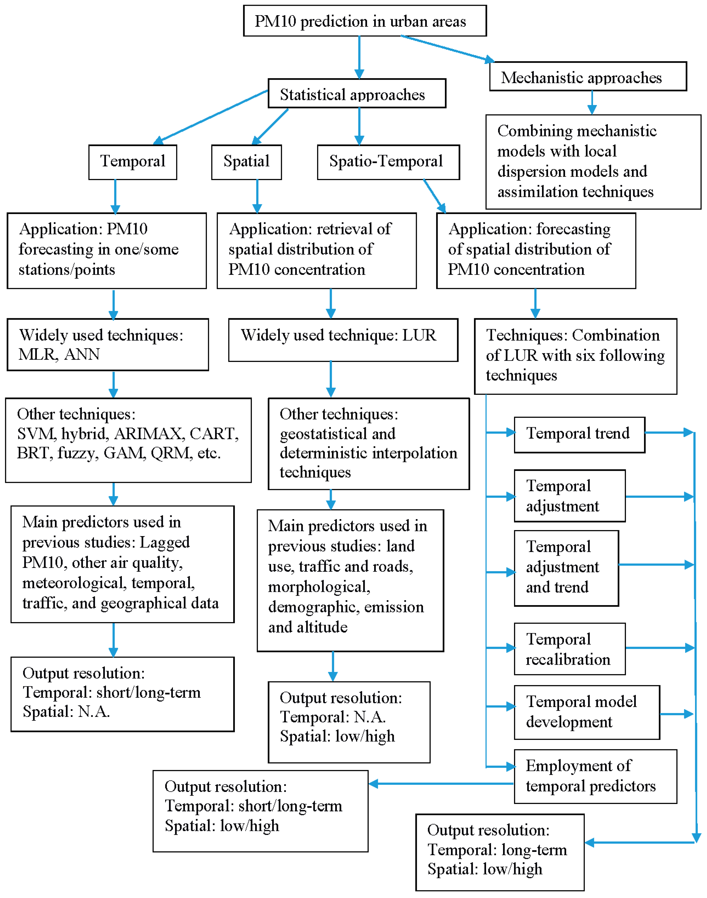
- Temporal trend: The simplest method is the utilization of the temporal trend of the air pollutant, derived from the local background monitoring stations, for the adjustment of LUR results for past years. The disadvantage of this technique is that the trend of the monitoring station is extended throughout the urban area [134,140]. This approach is easy and it can be suitable if a representative fixed station is employed. However, a fixed station, which is affected by local air pollution sources (a non-representative station), cannot properly calibrate the pollutant concentration [74]. Taheri Shahraiyni et al. [141] presented a technique for the determination of the most representative stations in urban areas. Combining this new technique with temporal trend may lead to an appropriate spatio-temporal model for long-term variations of PM10.
- Temporal adjustment: Another approach is the temporal adjustment of the values of the model’s predictors. This approach has some disadvantages. Many predictors change very slowly over time (e.g., land use) and consequently, this approach only predicts long-term variations in PM10 levels. In addition, the temporal changes of the predictors do not necessarily reflect the temporal changes of the pollutants [134], and this method does not account for changes in the relationship between predictors and air pollutants [140].
- Temporal adjustment and trend: The combination of the previous two approaches (temporal adjustment and temporal trend) can be considered as an approach for spatio-temporal prediction of PM10. In this approach, the spatio-temporal PM10 concentration is first calculated by the temporal adjustment technique, and then the temporal trend is added to the developed model [140].
- Temporal recalibration: The change, or recalibration of the coefficients of the existing model, is another approach for the development of a suitable model for other times [134,140]. Mölter et al. [134] recalibrated the LUR model for calculation of annual spatial variations of PM10 in Manchester, UK, over a long period. They concluded that this technique allows for the extrapolation of the LUR model over a long period. Wang et al. [140] compared different approaches (approaches 1–4) for hindcast and forecast of NO and NO2 in Vancouver, Canada and showed that the best approach is the recalibration technique.
- Employment of temporal predictors: Although the previous approaches (approaches 1–5) derived a spatio-temporal PM10 model, they have been utilized for long-term variations of air pollutants, and accordingly are not useful for the derivation of short-term variations of PM10. Employment of temporal predictors enables the estimation of short-term variation of air pollutants, by the utilization of some short-term dynamic input variables in the spatio-temporal model. For example, Gryparis et al. [143] and Maynard et al. [144] employed the temporal, meteorological, location (latitude and longitude) and traffic variables, along with black carbon levels measured at one monitoring station, for the development of a daily black carbon model for Boston, USA. However, they did not consider land use parameters. Su et al. [145] incorporated meteorological parameters into LUR models and utilized them for hourly NO2 estimation in Vancouver, Canada. Alam and McNabola [39] utilized the daily traffic and meteorological parameters, temporal parameter, and transboundary air pollution, derived from back trajectory analysis and population density, as input variables of the different statistical techniques (MLR, NPR (Non-Parametric Regression), ANN) within the LUR conceptual framework for the spatial simulation of daily PM10 concentration in Vienna (Austria) and Dublin (Ireland). The results showed that ANN (Dublin: R2 = 0.51; Vienna: R2 = 0.66) outperforms MLR (Dublin: R2 = 0.38–0.43; Vienna: R2 = 0.35–0.39) and NPR (Dublin: R2 = 0.45; Vienna: R2 = 0.51). They showed that the utilization of a non-linear technique, instead of linear techniques, can lead to an acceptable level of accuracy.
7. Summary and Conclusions

Acknowledgments
Author Contributions
Conflicts of Interest
References
- Sarkar, S.; Khillare, P.S.; Jyethi, D.S.; Hasan, A.; Parween, M. Chemical speciation of respirable suspended particulate matter during a major firework festival in India. J. Hazard. Mater. 2010, 184, 321–330. [Google Scholar] [CrossRef] [PubMed]
- Brunelli, U.; Piazza, V.; Pignato, L.; Sorbello, F.; Vitabile, S. Two-days ahead prediction of daily maximum concentrations of SO2, O3, PM10, NO2, CO in the urban area of Palermo, Italy. Atmos. Environ. 2007, 41, 2967–2995. [Google Scholar] [CrossRef]
- Vautard, R.; Bessagnet, B.; Chin, M.; Menut, L. On the contribution of natural Aeolian sources to particulate matter concentrations in Europe: Testing hypotheses with a modelling approach. Atmos. Environ. 2005, 39, 3291–3303. [Google Scholar] [CrossRef]
- Ni, T.; Han, B.; Bai, Z. Source Apportionment of PM10 in Four Cities of Northeastern China. Aerosol Air Qual. Res. 2012, 12, 571–582. [Google Scholar] [CrossRef]
- Hooyberghs, J.; Mensink, C.; Dumont, G.; Fierens, F.; Brasseur, O. A neural network forecast for daily average PM10 concentrations in Belgium. Atmos. Environ. 2005, 39, 3279–3289. [Google Scholar] [CrossRef]
- Maricq, M.M. Chemical characterization of particulate emissions from diesel engines: A review. J. Aerosol Sci. 2007, 38, 1079–1118. [Google Scholar] [CrossRef]
- Amato, F.; Pandolfi, M.; Moreno, T.; Furger, M.; Pey, J.; Alastuey, A.; Bukowiecki, N.; Prevot, A.S.H.; Baltensperger, U.; Querol, X. Sources and variability of inhalable road dust particles in three European cities. Atmos. Environ. 2011, 45, 6777–6787. [Google Scholar] [CrossRef]
- Lenschow, P.; Abraham, H.J.; Kutzner, K.; Lutz, M.; Preuß, J.D.; Reichenbächer, W. Some ideas about the sources of PM10. Atmos. Environ. 2001, 35, S23–S33. [Google Scholar] [CrossRef]
- Keary, J.; Jennings, S.G.; O’connor, T.C.; McManus, B.; Lee, M. PM10 concentration measurements in Dublin city. Environ. Monit. Assess. 1998, 52, 3–18. [Google Scholar] [CrossRef]
- Hoek, G.; Brunekreef, B.; Goldbohm, S.; Fischer, P.; van den Brandt, P.A. Association between mortality and indicators of traffic-related air pollution in the Netherlands: A cohort study. Lancet 2002, 360, 1203–1209. [Google Scholar] [CrossRef]
- Querol, X.; Alastuey, A.; Ruiz, C.R.; Artiñano, B.; Hansson, H.C.; Harrison, R.M.; Buringh, E.; ten Brink, H.M.; Lutz, M.; Bruckmann, P.; et al. Speciation and origin of PM10 and PM2.5 in selected European cities. Atmos. Environ. 2004, 38, 6547–6555. [Google Scholar] [CrossRef]
- Querol, X.; Alastuey, A.; Viana, M.M.; Rodriguez, S.; Artiñano, B.; Salvador, P.; Garcia do Santos, S.; Fernandez Patier, R.; Ruiz, C.R.; de la Rosa, J.; et al. Speciation and origin of PM10 and PM2.5 in Spain. J. Aerosol Sci. 2004, 35, 1151–1172. [Google Scholar] [CrossRef]
- Hueglin, C.; Gehrig, R.; Baltensperger, U.; Gysel, M.; Monn, C.; Vonmont, H. Chemical characterisation of PM2. 5, PM10 and coarse particles at urban, near-city and rural sites in Switzerland. Atmos. Environ. 2005, 39, 637–651. [Google Scholar] [CrossRef]
- Rauterberg-Wulff, A.; Lutz, M.; Nulis, E.; Reichenbacher, W.; Kettschau, A.; Schlickum, V.; Kerschbaumer, A.; Couturier, G.; Jarnott, F.; Gerike, S.; et al. Berlin’s Air Quality Plan 2011 to 2017; Senate Department for Urban Development and Environmental Communication: Berlin, Germany, 2013; p. 227. (In German) [Google Scholar]
- Khoder, M.I. Atmospheric conversion of sulfur dioxide to particulate sulfate and nitrogen dioxide to particulate nitrate and gaseous nitric acid in an urban area. Chemosphere 2002, 49, 675–684. [Google Scholar] [CrossRef]
- Tsai, Y.I.; Chen, C.L. Atmospheric aerosol composition and source apportionments to aerosol in southern Taiwan. Atmos. Environ. 2006, 40, 4751–4763. [Google Scholar] [CrossRef]
- Glinianaia, S.V.; Rankin, J.; Bell, R.; Pless-Mulloli, T.; Howel, D. Particulate air pollution and fetal health: A systematic review of the epidemiologic evidence. Epidemiology 2004, 15, 36–45. [Google Scholar] [CrossRef] [PubMed]
- Šrám, R.J.; Binková, B.; Dejmek, J.; Bobak, M. Ambient air pollution and pregnancy outcomes: A review of the literature. Environ. Health Persp. 2005, 113, 375–382. [Google Scholar] [CrossRef]
- Samet, J.M.; Zeger, S.L.; Dominici, F.; Curriero, F.; Coursac, I.; Dockery, D.W.; Schwartz, J.; Zanobetti, A. The National Morbidity, Mortality, and Air Pollution Study. Part II: Morbidity and Mortality from Air Pollution in the United States; Research Report, 94; Health Effects Institute: Cambridge, MA, USA, 2000. [Google Scholar]
- Dockery, D.W.; Pope, C.A.; Xu, X.; Spengler, J.D.; Ware, J.H.; Fay, M.E.; Ferris, B.G.; Speizer, F.E. An association between air pollution and mortality in six US cities. New Engl. J. Med. 1993, 329, 1753–1759. [Google Scholar] [CrossRef] [PubMed]
- Pope, C.A.; Thun, M.J.; Namboodiri, M.M.; Dockery, D.W.; Evans, J.S.; Speizer, F.E.; Heath, C.W., Jr. Particulate air pollution as a predictor of mortality in a prospective study of US adults. Am. J. Resp. Crit. Care Med. 1995, 151, 669–674. [Google Scholar] [CrossRef] [PubMed]
- Pope, C.A.; Burnett, R.T.; Thun, M.J.; Calle, E.E.; Krewski, D.; Ito, K.; Thurston, G.D. Lung cancer, cardiopulmonary mortality, and long-term exposure to fine particulate air pollution. J. Am. Med. Assoc. 2002, 287, 1132–1141. [Google Scholar] [CrossRef]
- Pope, C.A.; Dockery, D.W. Health effects of fine particulate air pollution: Lines that connect. J. Air Waste Manag. Assoc. 2006, 56, 709–742. [Google Scholar] [CrossRef] [PubMed]
- Chow, J.C.; Watson, J.G.; Mauderly, J.L.; Costa, D.L.; Wyzga, R.E.; Vedal, S.; Hidy, G.M.; Altshuler, S.L.; Marrack, D.; Heuss, J.M.; et al. Health effects of fine particulate air pollution: Lines that connect. J. Air Waste Manag. Assoc. 2006, 56, 1368–1380. [Google Scholar] [CrossRef] [PubMed]
- Sanhueza, P.; Vargas, C.; Mellado, P. Impact of air pollution by fine particulate matter (PM10) on daily mortality in Temuco, Chile. Rev. Med. Chile 2006, 134, 754–761. [Google Scholar] [PubMed]
- Sanhueza, P.A.; Torreblanca, M.A.; Diaz-Robles, L.A.; Schiappacasse, L.N.; Silva, M.P.; Astete, T.D. Particulate air pollution and health effects for cardiovascular and respiratory causes in Temuco, Chile: A wood-smoke-polluted urban area. J. Air Waste Manag. Assoc. 2009, 59, 1481–1488. [Google Scholar] [CrossRef] [PubMed]
- Dockery, D.W.; Pope, C.A. Acute respiratory effects of particulate air pollution. Annu. Rev. Publ. Health 1994, 15, 107–132. [Google Scholar] [CrossRef] [PubMed]
- Schwartz, J.; Dockery, D.W.; Neas, L.M. Is daily mortality associated specifically with fine particles? J. Air Waste Manag. Assoc. 1996, 46, 927–939. [Google Scholar] [CrossRef] [PubMed]
- Katsouyanni, K.; Touloumi, G.; Spix, C.; Schwartz, J.; Balducci, F.; Medina, S.; Rossi, G.; Ponka, A.; Schouten, J.P.; Anderson, H.R.; et al. Short term effects of ambient sulphur dioxide and particulate matter on mortality in 12 European cities: Results from time series data from the APHEA project. BMJ 1997, 314, 1658–1663. [Google Scholar] [CrossRef] [PubMed]
- European Union. Directive 2008/50/EC of the European parliament and of the council of 21 May 2008 on ambient air quality and cleaner air for Europe. Off. J. Eur. Union 2008, L152/1, 1–44. [Google Scholar]
- Baklanov, A.; Hänninen, O.; Slørdal, L.H.; Kukkonen, J.; Bjergene, N.; Fay, B.; Finardi, S.; Hoe, S.C.; Jantunen, M.; Karppinen, A.; et al. Integrated systems for forecasting urban meteorology, air pollution and population exposure. Atmos. Chem. Phys. 2007, 7, 855–874. [Google Scholar] [CrossRef]
- Stadlober, E.; Hörmann, S.; Pfeiler, B. Quality and performance of a PM10 daily forecasting model. Atmos. Environ. 2008, 42, 1098–1109. [Google Scholar] [CrossRef]
- Paschalidou, A.K.; Karakitsios, S.; Kleanthous, S.; Kassomenos, P.A. Forecasting hourly PM10 concentration in Cyprus through artificial neural networks and multiple regression models: Implications to local environmental management. Environ. Sci. Pollut. Res. 2011, 18, 316–327. [Google Scholar] [CrossRef] [PubMed]
- Diaz-Robles, L.A.; Ortega, J.C.; Fu, J.S.; Reed, G.D.; Chow, J.C.; Watson, J.G.; Moncada-Herrera, J.A. A hybrid ARIMA and artificial neural networks model to forecast particulate matter in urban areas: The case of Temuco, Chile. Atmos. Environ. 2008, 42, 8331–8340. [Google Scholar] [CrossRef]
- Kukkonen, J.; Partanen, L.; Karppinen, A.; Walden, J.; Kartastenpää, R.; Aarnio, P.; Koskentalo, T.; Berkowicz, R. Evaluation of the OSPM model combined with an urban background model against the data measured in 1997 in Runeberg Street, Helsinki. Atmos. Environ. 2003, 37, 1101–1112. [Google Scholar] [CrossRef]
- Hrust, L.; Klaić, Z.B.; Križan, J.; Antonić, O.; Hercog, P. Neural network forecasting of air pollutants hourly concentrations using optimised temporal averages of meteorological variables and pollutant concentrations. Atmos. Environ. 2009, 43, 5588–5596. [Google Scholar] [CrossRef]
- Goyal, P.; Chan, A.T.; Jaiswal, N. Statistical models for the prediction of respirable suspended particulate matter in urban cities. Atmos. Environ. 2006, 40, 2068–2077. [Google Scholar] [CrossRef]
- Jakeman, A.J.; Simpson, R.W.; Taylor, J.A. Modeling distributions of air pollutant concentrations– III. The hybrid deterministic-statistical distribution approach. Atmos. Environ. 1988, 22, 163–174. [Google Scholar] [CrossRef]
- Alam, M.S.; McNabola, A. Exploring the modeling of spatiotemporal variations in ambient air pollution within the land use regression framework: Estimation of PM10 concentrations on a daily basis. J. Air Waste Manag. Assoc. 2015, 65, 628–640. [Google Scholar] [CrossRef] [PubMed]
- Chang, J.C.; Hanna, S.R. Air quality model performance evaluation. Meteorol. Atmos. Phys. 2004, 87, 167–196. [Google Scholar] [CrossRef]
- Vautard, R.; Builtjes, P.H.J.; Thunis, P.; Cuvelier, C.; Bedogni, M.; Bessagnet, B.; Honore´, C.; Moussiopoulos, N.; Pirovano, G.; Schaap, M.; et al. Evaluation and intercomparison of Ozone and PM10 simulations by several chemistry transport models over four European cities within the CityDelta project. Atmos. Environ. 2007, 41, 173–188. [Google Scholar] [CrossRef]
- Borrego, C.; Monteiro, A.; Ferreira, J.; Miranda, A.I.; Costa, A.M.; Carvalho, A.C.; Lopes, M. Procedures for estimation of modelling uncertainty in air quality assessment. Environ. Int. 2008, 34, 613–620. [Google Scholar] [CrossRef] [PubMed]
- Stern, R.; Builtjes, P.; Schaap, M.; Timmermans, R.; Vautard, R.; Hodzic, A.; Memmesheimer, M.; Feldmann, H.; Renner, E.; Wolke, R.; et al. A model inter-comparison study focusing on episodes with elevated PM10 concentrations. Atmos. Environ. 2008, 42, 4567–4588. [Google Scholar] [CrossRef]
- Denby, B.; Schaap, M.; Segers, A.; Builtjes, P.; Horalek, J. Comparison of two data assimilation methods for assessing PM10 exceedances on the European scale. Atmos. Environ. 2008, 42, 7122–7134. [Google Scholar] [CrossRef]
- Konovalov, I.B.; Beekmann, M.; Meleux, F.; Dutot, A.; Foret, G. Combining deterministic and statistical approaches for PM10 forecasting in Europe. Atmos. Environ. 2009, 43, 6425–6434. [Google Scholar] [CrossRef]
- Borrego, C.; Monteiro, A.; Pay, M.T.; Ribeiro, I.; Miranda, A.I.; Basart, S.; Baldasano, J.M. How bias-correction can improve air quality forecasts over Portugal. Atmos. Environ. 2011, 45, 6629–6641. [Google Scholar] [CrossRef] [Green Version]
- Akita, Y.; Baldasano, J.M.; Beelen, R.; Cirach, M.; de Hoogh, K.; Hoek, G.; Nieuwenhuijsen, M.; Serre, M.L.; de Nazelle, A. Large scale air pollution estimation method combining land use regression and chemical transport modeling in a geostatistical framework. Environ. Sci. Technol. 2014, 48, 4452–4459. [Google Scholar] [CrossRef] [PubMed] [Green Version]
- Hamm, N.A.S.; Finley, A.O.; Schaap, M.; Stein, A. A spatially varying coefficient model for mapping PM10 air quality at the European scale. Atmos. Environ. 2015, 102, 393–405. [Google Scholar] [CrossRef]
- Van de Kassteele, J.; Velders, G.J.M. Uncertainty assessment of local NO2 concentrations derived from error-in-variable external drift Kriging and its relationship to the 2010 air quality standard. Atmos. Environ. 2006, 40, 2583–2595. [Google Scholar] [CrossRef]
- Duyzer, J.; van den Hout, D.; Zandveld, P.; van Ratingen, S. Representativeness of air quality monitoring networks. Atmos. Environ. 2015, 104, 88–101. [Google Scholar] [CrossRef]
- Fernando, H.J.S.; Mammarella, M.C.; Grandoni, C.; Fedele, P.; di Marco, R.; Dimitrova, R.; Hyde, P. Forecasting PM10 in metropolitan areas: Efficacy of neural networks. Environ. Pollut. 2012, 163, 62–67. [Google Scholar] [CrossRef] [PubMed]
- Slini, T.; Kaprara, A.; Karatzas, K.; Moussiopoulos, N. PM10 forecasting for Thessaloniki, Greece. Environ. Model. Softw. 2006, 21, 559–565. [Google Scholar] [CrossRef]
- Harrison, R.M.; Deacon, A.R.; Jones, M.R.; Appleby, R.S. Sources and processes affecting concentrations of PM10 and PM2.5 particulate matter in Birmingham (U.K.). Atmos. Environ. 1997, 31, 4103–4117. [Google Scholar] [CrossRef]
- Hubbard, M.C.; Cobourn, W.G. Development of a regression model to forecast ground-level ozone concentration in Louisville, KY. Atmos. Environ. 1998, 32, 2637–2647. [Google Scholar] [CrossRef]
- Papanastasiou, D.K.; Melas, D. Statistical characteristics of ozone and PM10 levels in a medium-sized Mediterranean city. Int. J. Environ. Pollut. 2008, 36, 127–138. [Google Scholar] [CrossRef]
- Papanastasiou, D.K.; Melas, D.; Kioutsioukis, I. Development and assessment of neural network and multiple regression models in order to predict PM10 levels in a medium-sized Mediterranean city. Water Air Soil Pollut. 2007, 182, 325–334. [Google Scholar] [CrossRef]
- Sayegh, A.S.; Munir, S.; Habeebullah, T.M. Comparing the performance of statistical models for predicting PM10 concentrations. Aerosol Air Qual. Res. 2014, 14, 653–665. [Google Scholar] [CrossRef]
- Grivas, G.; Chaloulakou, A. Artificial neural network models for prediction of PM10 hourly concentrations, in the Greater Area of Athens, Greece. Atmos. Environ. 2006, 40, 1216–1229. [Google Scholar] [CrossRef]
- Perez, P.; Reyes, J. Prediction of maximum of 24-h average of PM10 concentrations 30 h in advance in Santiago, Chile. Atmos. Environ. 2002, 36, 4555–4561. [Google Scholar] [CrossRef]
- Chen, L.; Bai, Z.; Kong, S.; Han, B.; You, Y.; Ding, X.; Du, S.; Liu, A. A land use regression for predicting NO2 and PM10 concentrations in different seasons in Tianjin region, China. J. Environ. Sci. 2010, 22, 1364–1373. [Google Scholar] [CrossRef]
- Kim, B.M.; Teffera, S.; Zeldin, M.D. Characterization of PM2.5 and PM10 in the South Coast air basin of Southern California: Part 1—Spatial variations. J. Air Waste Manag. Assoc. 2000, 50, 2034–2044. [Google Scholar] [CrossRef] [PubMed]
- Taheri Shahraiyni, H.; Sodoudi, S.; Cubasch, U.; Kerschbaumer, A. The influence of the plants on the decrease of air pollutants (Case study: Particulate matter in Berlin). In Presented at the Euro-American Conference for Academic Disciplines, Paris, France, 13–16 April 2015.
- Zhang, G.P. Time series forecasting using a hybrid ARIMA and neural network model. Neurocomputing 2003, 50, 159–175. [Google Scholar] [CrossRef]
- Chelani, A.B.; Gajghate, D.G.; Hasan, M.Z. Prediction of ambient PM10 and toxic metals using artificial neural networks. J. Air Waste Manag. Assoc. 2002, 52, 805–810. [Google Scholar] [CrossRef] [PubMed]
- McKendry, I.G. Evaluation of artificial neural networks for fine particulate pollution (PM10 and PM2.5) forecasting. J. Air Waste Manag. Assoc. 2002, 52, 1096–1101. [Google Scholar] [CrossRef] [PubMed]
- Chaloulakou, A.; Grivas, G.; Spyrellis, N. Neural network and multiple regression models for PM10 prediction in Athens: A comparative assessment. J. Air Waste Manag. Assoc. 2003, 53, 1183–1190. [Google Scholar] [CrossRef] [PubMed]
- Lu, W.Z.; Wang, W.J.; Wang, X.K.; Yan, S.H.; Lam, J.C. Potential assessment of a neural network model with PCA/RBF approach for forecasting pollutant trends in Mong Kok urban air, Hong Kong. Environ. Res. 2004, 96, 79–87. [Google Scholar] [CrossRef] [PubMed]
- Corani, G. Air quality prediction in Milan: Feed-forward neural networks, pruned neural networks and lazy learning. Ecol. Model. 2005, 185, 513–529. [Google Scholar] [CrossRef]
- Perez, P.; Reyes, J. An integrated neural network model for PM10 forecasting. Atmos. Environ. 2006, 40, 2845–2851. [Google Scholar] [CrossRef]
- Cai, M.; Yin, Y.; Xie, M. Prediction of hourly air pollutant concentrations near urban arterials using artificial neural network approach. Transp. Res. Part D Transp. Environ. 2009, 14, 32–41. [Google Scholar] [CrossRef]
- Perez, P. Combined model for PM10 forecasting in a large city. Atmos. Environ. 2012, 60, 271–276. [Google Scholar] [CrossRef]
- Nejadkoorki, F.; Baroutian, S. Forecasting extreme PM10 concentrations using artificial neural networks. Int. J. Environ. Res. 2012, 6, 277–284. [Google Scholar]
- Popescu, M.; Ilie, C.; Panaitescu, L.; Lungu, M.L.; Ilie, M.; Lungu, D. Artificial neural networks forecasting of the PM10 quantity in London considering the Harwell and Rochester Stoke PM10 measurements. J. Environ. Prot. Ecol. 2013, 14, 1473–1481. [Google Scholar]
- Liu, W.; Li, X.; Chen, Z.; Zeng, G.; León, T.; Liang, J.; Huang, G.; Gao, Z.; Jiao, S.; He, X.; et al. Land use regression models coupled with meteorology to model spatial and temporal variability of NO2 and PM10 in Changsha, China. Atmos. Environ. 2015, 116, 272–280. [Google Scholar] [CrossRef]
- Nagendra, S.S.; Khare, M. Artificial neural network approach for modelling nitrogen dioxide dispersion from vehicular exhaust emissions. Ecol. Model. 2006, 190, 99–115. [Google Scholar] [CrossRef]
- Aldrin, M.; Haff, I.H. Generalised additive modelling of air pollution, traffic volume and meteorology. Atmos. Environ. 2005, 39, 2145–2155. [Google Scholar] [CrossRef]
- Suárez Sánchez, A.; Nieto, P.G.; Fernández, P.R.; del Coz Díaz, J.J.; Iglesias-Rodríguez, F.J. Application of an SVM-based regression model to the air quality study at local scale in the Avilés urban area (Spain). Math. Comput. Model. 2011, 54, 1453–1466. [Google Scholar] [CrossRef]
- Munir, S.; Habeebullah, T.M.; Seroji, A.R.; Morsy, E.A.; Mohammed, A.M.; Saud, W.A.; Abdou, A.E.A.; Awad, A.H. Modeling particulate matter concentrations in makkah, applying a statistical modeling approach. Aerosol Air Qual. Res. 2013, 13, 901–910. [Google Scholar] [CrossRef]
- Suárez Sánchez, A.; García Nieto, P.J.; Iglesias-Rodríguez, F.J.; Vilan Vilan, J.A. Nonlinear air quality modeling using support vector machines in Gijón urban area (Northern Spain) at local scale. Int. J. Nonlinear Sci. Numer. Simul. 2013, 14, 291–305. [Google Scholar] [CrossRef]
- Box, G.E.P.; Jenkins, G.M. Time Series Analysis, Forecasting and Control; Holden-Day: San Francisco, CA, USA, 1970; p. 575. [Google Scholar]
- Cortes, C.; Vapnik, V. Support-vector networks. Mach. Learn. 1995, 20, 273–297. [Google Scholar] [CrossRef]
- Bruzzone, L.; Melgani, F. Robust multiple estimator systems for the analysis of biophysical parameters from remotely sensed data. IEEE Trans.Geosci. Remote Sens. 2005, 43, 159–174. [Google Scholar] [CrossRef]
- Raimondo, G.; Montuori, A.; Moniaci, W.; Pasero, E.; Almkvist, E. A machine learning tool to forecast PM10 level. In Proceedings of the AMS 87th Annual Meeting, San Antonio, TX, USA, 13–18 January 2007.
- Sotomayor-Olmedo, A.; Aceves-Fernández, M.A.; Gorrostieta-Hurtado, E.; Pedraza-Ortega, C.; Ramos-Arreguín, J.M.; Vargas-Soto, J.E. Forecast urban air pollution in Mexico City by using support vector machines: A kernel performance approach. Int. J. Intell. Sci. 2013, 3, 126–135. [Google Scholar] [CrossRef]
- Hastie, T.J.; Tibshirani, R.J. Generalized Additive Models; Chapman and Hall/CRC: London, UK, 1990. [Google Scholar]
- Koenker, R. Quantile Regression; No. 38; Cambridge University Press: Cambridge, UK, 2005. [Google Scholar]
- Breiman, L.; Friedman, J.H.; Olshen, R.; Stone, C.J. Classification and Regression Trees; Wadsworth: Belmont, CA, USA, 1984. [Google Scholar]
- Yetilmezsoy, K.; Abdul-Wahab, S.A. A prognostic approach based on fuzzy-logic methodology to forecast PM10 levels in Khaldiya residential area, Kuwait. Aerosol Air Qual. Res. 2012, 12, 1217–1236. [Google Scholar] [CrossRef]
- Diem, J.E.; Comrie, A.C. Predictive mapping of air pollution involving sparse spatial observations. Environ. Pollut. 2002, 119, 99–117. [Google Scholar] [CrossRef]
- Kanakiya, R.S.; Singh, S.K.; Shah, U. GIS Application for spatial and temporal analysis of the air pollutants in urban area. Int. J. Adv. Remote Sens. GIS 2015, 4, 1120–1129. [Google Scholar]
- Tuna, F.; Buluç, M. Analysis of PM10 pollutant in Istanbul by using Kriging and IDW methods: Between 2003 and 2012. Int. J. Comput. Inf. Technol. 2015, 4, 170–175. [Google Scholar]
- Dimitrova, R.; Lurponglukana, N.; Fernando, H.J.S.; Runger, G.C.; Hyde, P.; Hedquist, B.C.; Johnson, W. Relationship between particulate matter and childhood asthma-basis of a future warning system for Central Phoenix. Atmos. Chem. Phys. Discuss. 2011, 11, 28627–28661. [Google Scholar] [CrossRef]
- Lertxundi-Manterola, A.; Saez, M. Modelling of nitrogen dioxide (NO2) and fine particulate matter (PM10) air pollution in the metropolitan areas of Barcelona and Bilbao, Spain. Environmetrics 2009, 20, 477–493. [Google Scholar] [CrossRef]
- Beelen, R.; Hoek, G.; Pebesma, E.; Vienneau, D.; de Hoogh, K.; Briggs, D.J. Mapping of background air pollution at a fine spatial scale across the European Union. Sci. Total Environ. 2009, 407, 1852–1867. [Google Scholar] [CrossRef] [PubMed]
- Pope, R.; Wu, J. Characterizing air pollution patterns on multiple time scales in urban areas: A landscape ecological approach. Urban Ecosyst. 2014, 17, 855–874. [Google Scholar] [CrossRef]
- Kottur, S.V.; Mantha, S.S. An integrated model using Artificial Neural Network (ANN) and Kriging for forecasting air pollutants using meteorological data. Int. J. Adv. Res. Comput. Commun. Eng. 2015, 4, 146–152. [Google Scholar] [CrossRef]
- Liao, D.; Peuquet, D.J.; Duan, Y.; Whitsel, E.A.; Dou, J.; Smith, R.L.; Heiss, G. GIS approaches for the estimation of residential-level ambient PM concentrations. Environ. Health Persp. 2006, 114, 1374–1380. [Google Scholar] [CrossRef]
- Briggs, D.J.; Collins, S.; Elliott, P.; Fischer, P.; Kingham, S.; Lebret, E.; van der Veen, A. Mapping urban air pollution using GIS: A regression-based approach. Int. J. Geogr. Inf. Sci. 1997, 11, 699–718. [Google Scholar] [CrossRef]
- Aguilera, I.; Sunyer, J.; Fernández-Patier, R.; Esteban, R.G.; Bomboi, T.; Alvarez-Pedrerol, M. Using land-use regression modeling to estimate exposure to VOCs in a cohort of pregnant women. Epidemiology 2007, 18, S42–S43. [Google Scholar]
- Briggs, D. The role of GIS: Coping with space (and time) in air pollution exposure assessment. J. Toxicol. Environ. Health Part A 2005, 68, 1243–1261. [Google Scholar] [CrossRef] [PubMed]
- Hewitt, C.N. Spatial variations in nitrogen dioxide concentration in an urban area. Atmos. Environ. 1991, 25, 429–434. [Google Scholar] [CrossRef]
- Myers, D.E. Interpolation and estimation with spatially located data. Chemom. Intell. Lab. Syst. 1991, 11, 209–228. [Google Scholar] [CrossRef]
- Liu, L.J.S.; Rossini, A.J. Use of Kriging models to predict 12-hour mean ozone concentrations in metropolitan Toronto—A pilot study. Environ. Int. 1996, 22, 677–692. [Google Scholar] [CrossRef]
- Diem, J.E. A critical examination of ozone mapping from a spatial-scale perspective. Environ. Pollut. 2003, 125, 369–383. [Google Scholar] [CrossRef]
- Vicedo-Cabrera, A.M.; Biggeri, A.; Grisotto, L.; Barbone, F.; Catelan, D. A Bayesian Kriging model for estimating residential exposure to air pollution of children living in a high-risk area in Italy. Geospat. Health 2013, 8, 87–95. [Google Scholar] [CrossRef] [PubMed]
- Carnevale, C.; Decanini, E.; Volta, M. Design and validation of a multiphase 3D model to simulate tropospheric pollution. Sci. Total Environ. 2008, 390, 166–176. [Google Scholar] [CrossRef] [PubMed]
- Singh, V.; Carnevale, C.; Finzi, G.; Pisoni, E.; Volta, M. A cokriging based approach to reconstruct air pollution maps, processing measurement station concentrations and deterministic model simulations. Environ. Model. Softw. 2011, 26, 778–786. [Google Scholar] [CrossRef]
- Carnevale, C.; Finzi, G.; Pisoni, E.; Singh, V.; Volta, M. An integrated air quality forecast system for a metropolitan area. J. Environ. Monit. 2011, 13, 3437–3447. [Google Scholar] [CrossRef] [PubMed]
- Pollice, A.; Lasinio, G.J. Spatiotemporal analysis of the PM10 concentration over the Taranto area. Environ. Monit. Assess. 2010, 162, 177–190. [Google Scholar] [CrossRef] [PubMed]
- Le, N.Z.; Zidek, J.V. Statistical Analysis of Environmental Space-Time Processes; Springer Science & Business Media: New York, NY, USA, 2006. [Google Scholar]
- Park, N.W. Time-series mapping of PM10 concentration using multi-gaussian space-time Kriging: A case study in the Seoul metropolitan area, Korea. Adv. Meteorol. 2015, 1–10. [Google Scholar] [CrossRef]
- Montero, J.M.; Fernández-Avilés, G. Functional Kriging prediction of pollution series: The geostatistical alternative for spatially-fixed data. Estudios Econ. Apl. 2015, 33, 145–174. [Google Scholar]
- Hoek, G.; Beelen, R.; de Hoogh, K.; Vienneau, D.; Gulliver, J.L.; Fischer, P.; Briggs, D. A review of land-use regression models to assess spatial variation of outdoor air pollution. Atmos. Environ. 2008, 42, 7561–7578. [Google Scholar] [CrossRef]
- Jerrett, M.; Arain, A.; Kanaroglou, P.; Beckerman, B.; Potoglou, D.; Sahsuvaroglu, T.; Morrison, J.; Giovis, C. A review and evaluation of intraurban air pollution exposure models. J. Expo. Sci. Environ. Epidemiol. 2005, 15, 185–204. [Google Scholar] [CrossRef] [PubMed]
- Ryan, P.H.; LeMasters, G.K. A review of land-use regression models for characterizing intraurban air pollution exposure. Inhal. Toxicol. 2007, 19 (Suppl. 1), 127–133. [Google Scholar] [CrossRef] [PubMed]
- Gilbert, N.L.; Goldberg, M.S.; Beckerman, B.; Brook, J.R.; Jerrett, M. Assessing spatial variability of ambient nitrogen dioxide in Montreal, Canada, with a land-use regression model. J. Air Waste Manag. Assoc. 2005, 55, 1059–1063. [Google Scholar] [CrossRef] [PubMed]
- Ross, Z.; English, P.B.; Scalf, R.; Gunier, R.; Smorodinsky, S.; Wall, S.; Jerrett, M. Nitrogen dioxide prediction in Southern California using land use regression modeling: Potential for environmental health analyses. J. Exp. Sci. Environ. Epidemiol. 2006, 16, 106–114. [Google Scholar] [CrossRef] [PubMed]
- Hochadel, M.; Heinrich, J.; Gehring, U.; Morgenstern, V.; Kuhlbusch, T.; Link, E.; Wichmann, H.E.; Krämer, U. Predicting long-term average concentrations of traffic-related air pollutants using GIS-based information. Atmos. Environ. 2006, 40, 542–553. [Google Scholar] [CrossRef]
- Henderson, S.B.; Beckerman, B.; Jerrett, M.; Brauer, M. Application of land use regression to estimate long-term concentrations of traffic-related nitrogen oxides and fine particulate matter. Environ. Sci. Technol. 2007, 41, 2422–2428. [Google Scholar] [CrossRef] [PubMed]
- Chen, L.; Bai, Z.; Kong, S.; You, Y.; Han, B.; Han, D.; Li, Z. Application of land use regression for estimating concentrations of major outdoor air pollutants in Jinan, China. J. Zhejiang Univ. Sci. A 2010, 11, 857–867. [Google Scholar]
- Dons, E.; van Poppel, M.; Kochan, B.; Wets, G.; Panis, L.I. Modeling temporal and spatial variability of traffic-related air pollution: Hourly land use regression models for black carbon. Atmos. Environ. 2013, 74, 237–246. [Google Scholar] [CrossRef]
- Dons, E.; van Poppel, M.; Panis, L.I.; de Prins, S.; Berghmans, P.; Koppen, G.; Matheeussen, C. Land use regression models as a tool for short, medium and long term exposure to traffic related air pollution. Sci. Total Environ. 2014, 476–477, 378–386. [Google Scholar] [CrossRef] [PubMed]
- Tang, R.; Blangiardo, M.; Gulliver, J. Using building heights and street configuration to enhance intraurban PM10, NOx, and NO2 Land use regression models. Environ. Sci. Technol. 2013, 47, 11643–11650. [Google Scholar] [CrossRef] [PubMed]
- Gulliver, J.; de Hoogh, K.; Fecht, D.; Vienneau, D.; Briggs, D. Comparative assessment of GIS-based methods and metrics for estimating long-term exposures to air pollution. Atmos. Environ. 2011, 45, 7072–7080. [Google Scholar] [CrossRef]
- Eeftens, M.; Beelen, R.; de Hoogh, K.; Bellander, T.; Cesaroni, G.; Cirach, M.; Dons, E.; Sugiri, D.; Eriksen, K.; Hoek, G.; et al. Development of land use regression models for PM2.5, PM2.5 absorbance, PM10 and PM coarse in 20 European study areas; Results of the ESCAPE project. Environ. Sci. Technol. 2012, 46, 11195–11205. [Google Scholar] [CrossRef] [PubMed]
- Zhang, H.; Liu, Y.; Shi, R.; Yao, Q. Evaluation of PM10 forecasting based on the artificial neural network model and intake fraction in an urban area: A case study in Taiyuan City, China. J. Air Waste Manag. Assoc. 2013, 63, 755–763. [Google Scholar] [CrossRef] [PubMed]
- Amini, H.; Taghavi-Shahri, S.M.; Henderson, S.B.; Naddafi, K.; Nabizadeh, R.; Yunesian, M. Land use regression models to estimate the annual and seasonal spatial variability of sulfur dioxide and particulate matter in Tehran, Iran. Sci. Total Environ. 2014, 488–489, 343–353. [Google Scholar] [CrossRef] [PubMed]
- Lee, J.H.; Wu, C.F.; Hoek, G.; de Hoogh, K.; Beelen, R.; Brunekreef, B.; Chan, C.C. LUR models for particulate matters in the Taipei metropolis with high densities of roads and strong activities of industry, commerce and construction. Sci. Total Environ. 2015, 514, 178–184. [Google Scholar] [CrossRef] [PubMed]
- Li, X.; Liu, W.; Chen, Z.; Zeng, G.; Hu, C.; León, T.; Liang, J.; Huang, G.; Gao, Z.; Li, Z.; et al. The application of semicircular-buffer-based land use regression models incorporating wind direction in predicting quarterly NO2 and PM10 concentrations. Atmos. Environ. 2015, 103, 18–24. [Google Scholar] [CrossRef]
- Basagaña, X.; Rivera, M.; Aguilera, I.; Agis, D.; Bouso, L.; Elosua, R.; Foraster, M.; de Nazelle, A.; Nieuwenhuijsen, M.; Vila, J.; et al. Effect of the number of measurement sites on land use regression models in estimating local air pollution. Atmos. Environ. 2012, 54, 634–642. [Google Scholar] [CrossRef]
- Taheri Shahraiyni, H.; Sodoudi, S.; Cubasch, U. Determination the optimum number and positions of monitoring stations for proper spatial modeling of PM10 concentration in Berlin. In Proceedings of the European Geosciences Union General Assembly Meeting, Vienna, Austria, 27 April–2 May 2014.
- Hickey, H.R.; Rowe, W.D.; Skinner, F. A cost model for air quality monitoring systems. J. Air Pollut. Control Assoc. 1971, 21, 689–693. [Google Scholar] [CrossRef] [PubMed]
- Cocheo, C.; Sacco, P.; Ballesta, P.P.; Donato, E.; Garcia, S.; Gerboles, M.; Gombert, D.; McManus, B.; Patier, R.F.; Roth, R.; et al. Evaluation of the best compromise between the urban air quality monitoring resolution by diffusive sampling and resource requirements. J. Environ. Monit. 2008, 10, 941–950. [Google Scholar] [CrossRef] [PubMed]
- Mölter, A.; Lindley, S.; de Vocht, F.; Simpson, A.; Agius, R. Modelling air pollution for epidemiologic research—Part I: A novel approach combining land use regression and air dispersion. Sci. Total Environ. 2010, 408, 5862–5869. [Google Scholar] [CrossRef] [PubMed]
- Trujillo-Ventura, A.; Hugh Ellis, J. Multiobjective air pollution monitoring network design. Atmos. Environ. 1991, 25, 469–479. [Google Scholar] [CrossRef]
- Taheri Shahraiyni, H.; Sodoudi, S.; Kerschbaumer, A.; Cubasch, U. A new structure-identification scheme for ANFIS and its application for the simulation of virtual air-pollution monitoring-stations in urban areas. Eng. Appl. Artif. Intell. 2015, 41, 175–182. [Google Scholar] [CrossRef]
- Taheri Shahraiyni, H.; Sodoudi, S.; Kerschbaumer, A.; Cubasch, U. The development of a dense urban air pollution monitoring network. Atmos. Pollut. Res. 2015, 6, 904–915. [Google Scholar] [CrossRef]
- Dormann, C.F.; Elith, J.; Bacher, S.; Buchmann, C.; Carl, G.; Carré, G.; Marquéz, J.R.G.; Gruber, B.; Lafourcade, B.; Leitão, P.J.; et al. Collinearity: A review of methods to deal with it and a simulation study evaluating their performance. Ecography 2013, 36, 27–46. [Google Scholar] [CrossRef]
- Chatterjee, S.; Hadi, A.S. Regression Analysis by Example, 4th ed.; John Wiley & Sons: New York, NY, USA, 2006. [Google Scholar]
- Wang, R.; Henderson, S.B.; Sbihi, H.; Allen, R.W.; Brauer, M. Temporal stability of land use regression models for traffic-related air pollution. Atmos. Environ. 2013, 64, 312–319. [Google Scholar] [CrossRef]
- Taheri Shahraiyni, H.; Sodoudi, S.; Kerschbaumer, A.; Cubasch, U. New technique for ranking of air pollution monitoring stations in the urban areas based upon spatial representativity (Case study: PM monitoring stations in Berlin). Aerosol Air Qual. Res. 2015, 15, 743–748. [Google Scholar] [CrossRef]
- Gulliver, J.; Morris, C.; Lee, K.; Vienneau, D.; Briggs, D.; Hansell, A. Land use regression modeling to estimate historic (1962–1991) concentrations of black smoke and sulfur dioxide for Great Britain. Environ. Sci. Technol. 2011, 45, 3526–3532. [Google Scholar] [CrossRef] [PubMed]
- Gryparis, A.; Coull, B.A.; Schwartz, J.; Suh, H.H. Semiparametric latent variable regression models for spatiotemporal modelling of mobile source particles in the greater Boston area. J. R. Stat. Soc. Ser C Appl. Stat. 2007, 56, 183–209. [Google Scholar] [CrossRef]
- Maynard, D.; Coull, B.A.; Gryparis, A.; Schwartz, J. Mortality risk associated with short-term exposure to traffic particles and sulfates. Environ. Health Persp. 2007, 115, 751–755. [Google Scholar] [CrossRef] [PubMed]
- Su, J.G.; Brauer, M.; Ainslie, B.; Steyn, D.; Larson, T.; Buzzelli, M. An innovative land use regression model incorporating meteorology for exposure analysis. Sci. Total Environ. 2008, 390, 520–529. [Google Scholar] [CrossRef] [PubMed]
- Bechtel, B.; Zakšek, K.; Hoshyaripour, G. Downscaling land surface temperature in an urban area: A case study for Hamburg, Germany. Remote Sens. 2012, 4, 3184–3200. [Google Scholar] [CrossRef]
- Merbitz, H.; Fritz, S.; Schneider, C. Mobile measurements and regression modeling of the spatial particulate matter variability in an urban area. Sci. Total Environ. 2012, 438, 389–403. [Google Scholar] [CrossRef] [PubMed]
© 2016 by the authors; licensee MDPI, Basel, Switzerland. This article is an open access article distributed under the terms and conditions of the Creative Commons by Attribution (CC-BY) license (http://creativecommons.org/licenses/by/4.0/).
Share and Cite
Taheri Shahraiyni, H.; Sodoudi, S. Statistical Modeling Approaches for PM10 Prediction in Urban Areas; A Review of 21st-Century Studies. Atmosphere 2016, 7, 15. https://doi.org/10.3390/atmos7020015
Taheri Shahraiyni H, Sodoudi S. Statistical Modeling Approaches for PM10 Prediction in Urban Areas; A Review of 21st-Century Studies. Atmosphere. 2016; 7(2):15. https://doi.org/10.3390/atmos7020015
Chicago/Turabian StyleTaheri Shahraiyni, Hamid, and Sahar Sodoudi. 2016. "Statistical Modeling Approaches for PM10 Prediction in Urban Areas; A Review of 21st-Century Studies" Atmosphere 7, no. 2: 15. https://doi.org/10.3390/atmos7020015
APA StyleTaheri Shahraiyni, H., & Sodoudi, S. (2016). Statistical Modeling Approaches for PM10 Prediction in Urban Areas; A Review of 21st-Century Studies. Atmosphere, 7(2), 15. https://doi.org/10.3390/atmos7020015