Bias Correction for Retrieval of Atmospheric Parameters from the Microwave Humidity and Temperature Sounder Onboard the Fengyun-3C Satellite

Abstract

The microwave humidity and temperature sounder (MWHTS) on the Fengyun (FY)-3C satellite measures the outgoing radiance from the Earth’s surface and atmospheric constituents. MWHTS, which makes measurements in the isolated oxygen absorption line near 118 GHz and the vicinity of the strong water vapor absorption line around 183 GHz, can provide fine vertical distribution structures of both atmospheric humidity and temperature. However, in order to obtain the accurate soundings of humidity and temperature by physical retrieval methods, the bias between the observed and simulated radiance calculated by the radiative transfer model from the background or first guess profiles must be corrected. In this study, two bias correction methods are developed through the correlation analysis between MWHTS measurements and air mass identified by the first guess profiles of the physical inversion; one is the linear regression correction (LRC), and the other is the neural network correction (NNC), representing the linear and nonlinear relationships between MWHTS measurements and air mass, respectively. The correction methods have been applied to MWHTS observed brightness temperatures over the geographic area (180° W–180° E, 60° S–60° N). The corrected results are evaluated by the probability density function of the differences between corrected observations and simulated values and the root mean square errors (RMSE) with respect to simulated observations. The numerical results show that the NNC method has better performance, especially in MWHTS Channels 1 and 7–9, whose peak weight function heights are close to the surface. In order to assess the effects of bias correction methods proposed in this study on the retrieval accuracy, a one-dimensional variational system was built and applied to the MWHTS brightness temperatures to estimate the atmospheric temperature and humidity profiles. The retrieval results also show that NNC has better performance. An indication of the stability and robustness of the NNC method is given, which suggests that the NNC method has promising application perspectives in the physical retrieval.

1. Introduction

Atmospheric temperature and humidity profiles play important roles in a wide range of atmospheric applications, such as climate monitoring, weather forecasting, initialization and evaluation of numerical weather prediction (NWP) models, assessing the atmospheric stability and nowcasting the intense convective weather, to name a few, and will clearly continue to be important for the foreseeable future [1,2]. Take NWP models for example; accurate profiles of temperature and humidity are essential for model initialization. Taken as the first guess, which is used to start the iterative process in the radiances’ assimilation system, accurate profiles of temperature and humidity could help to speed up the convergence process of iteration and further improve the timeliness of NWP. Such profiles can be retrieved from observations taken by satellite-borne sounders. Microwave measurements are advantageous over visible or infrared because clouds do not absorb and scatter microwave radiation to the same degree [3]. This allows for microwave measurements of atmospheric parameters in most weather conditions and provides a substantial dataset [4]. The FY-3C satellite, launched in September 2013, is the second-generation polar-orbiting meteorological satellite. The MWHTS onboard FY-3C satellite has 15 channels at frequencies ranging from 89–191 GHz, which allows simultaneous retrieval of the atmospheric temperature and humidity profiles with good temporal and spatial sampling under clear and cloudy conditions [5]. MWHTS inherits most of the channels from its predecessors: the microwave humidity sounder onboard the FY-3A and FY-3B satellites. However, microwave humidity and temperature sounder (MWHTS) includes eight new temperature sounding channels centered at the 118.75-GHz oxygen absorption line, which are used in operation for the first time internationally, and two new water vapor sounding channels. Those channels provide more details of the vertical distribution structure of atmospheric temperature and humidity.

Although the development of atmospheric temperature and humidity profile measurement using satellite-borne microwave sounders has a history of over 50 years and the improvement of inversion approaches are actively continuing [6], the retrieval strategies can be put into two categories: statistical methods and physical methods. Statistical approaches essentially use a statistical relationship between the actual observations and the atmospheric state variables and do not take any physical models into account [7,8,9,10]. In essence, physical methods propagate a first guess of the atmospheric parameters through a radiative transfer model and an iterative scheme, numerical procedures to fit the simulated measurements to the satellite observations by updating the first guess at each iteration [11,12,13,14]. Physical methods are the basic way to improve the retrieval accuracy and have been widely adopted, since they have clear physical meanings. All of the physical methods employ either a minimum variance estimate or maximum likelihood estimate under the assumption that observations are unbiased and have Gaussian errors [15]. Any bias related to the instrument and the radiative transfer model should be taken into account when determining the appropriate weight of radiance data in the physical retrieval process; therefore, it must be quantified and removed. The bias in our study refers to systematic error rather than random error. In statistics, bias is a feature of the estimator, which, on average, over- or under-estimates the true value. For instance, a radiative transfer model that is always cold under certain circumstances is biased [16]. The appearance of biases in the observations and the radiative transfer model is due to systematic errors in any one (but generally a combination) of the following sources: the satellite sounder (e.g., poor calibration or adverse environmental effects); the radiative transfer model (e.g., errors in the physics, or spectroscopy, or from non-modeled atmospheric process); and errors in the background atmospheric parameters from some data sources (e.g., radiosonde observations, numerical weather prediction (NWP) analysis, climate re-analysis, etc.) [17]. Since the causes of bias are complicated and manifold, removing the bias using a statistical model whose calculating process is simple may be more popular. Many efforts based on statistical methods have been made to develop the bias correction scheme for the NWP radiances’ assimilation system and the physical retrieval system. These two systems are based on variational approaches, which have a similar cost function to find the optimal solution. Thus, they can share the same bias removal scheme. For microwave radiometer measurements, many previous studies have developed empirical correction methods, which remove the systemic biases by an empirical factor varying with instrument, radiative transfer model, observation conditions, etc. These methods have been applied to the Microwave Sounding Unit (MSU) and Advanced Microwave Sounding Unit (AMSU)-A/B [18,19,20]. Li et al. adjusted the AMSU-A/B observations or forward model calculations by statistical relationships between the radiances in the same channel, irrespective of the atmosphere state [21]. However, Kelly and Flobert, McMillin et al. and Uddstrom demonstrated that a successful bias correction scheme must take into account the spatially-varying and air mass-dependent characters of the radiance biases and proposed the scan correction, which correct the measurements of different scan angles relative to the nadir observation and the air-mass correction taking into account the air-mass-dependent character of the radiance biases. This two-step correction scheme has been applied to MSU, AMSU-A/B, the Special Sensor Microwave/Imager (SSM/I) and the Special Sensor Microwave Imager/Sounder (SSMIS) [22,23,24,25]. Based on air-mass correction, in the satellite radiances’ assimilation system, the adaptive bias correction scheme has been proposed, which can distinguish the observation biases from the biases in the background in order to prevent the analysis from drifting towards its own climate. This correction scheme is now widely used in the NWP radiances’ assimilation system [16,17,26,27]. However, all of these air mass correction schemes belong to the linear regression approach assuming that the relationship between the atmospheric state and radiance bias is linear. The methods may not represent their intrinsic features very well. Additionally, for the MWHTS, there are few research works on bias correction for the atmospheric parameters’ retrieval.

To correct the biases between observations and those simulated by the radiative transfer model in the physical retrieval procedure, for air-mass correction, the linear regression correction (LRC) and neural network correction (NNC), representing the linear and nonlinear relationships between the biases in MWHTS measurements and air mass, respectively, are proposed. In order to evaluate the performances of this two bias correction methods in the physical retrieval system, a one-dimensional variational retrieval system is built to retrieve atmospheric temperature and humidity profiles using MWHTS brightness temperatures. In addition, the tests of the stability and robustness of the correction method proposed in this study are carried out by different atmospheric conditions and different algorithm initialization conditions. This paper is organized as follows: Section 2 provides the major instrument characteristics of FY-3C/MWHTS. Brightness temperatures’ simulations by the radiative transfer model, LRC and NNC approaches for the air mass correction and scan correction are described in Section 3. The retrieval system for MWHTS data is built in Section 4. The proposed bias correction approaches are evaluated in Section 5. Finally, the conclusions are summarized in Section 6.

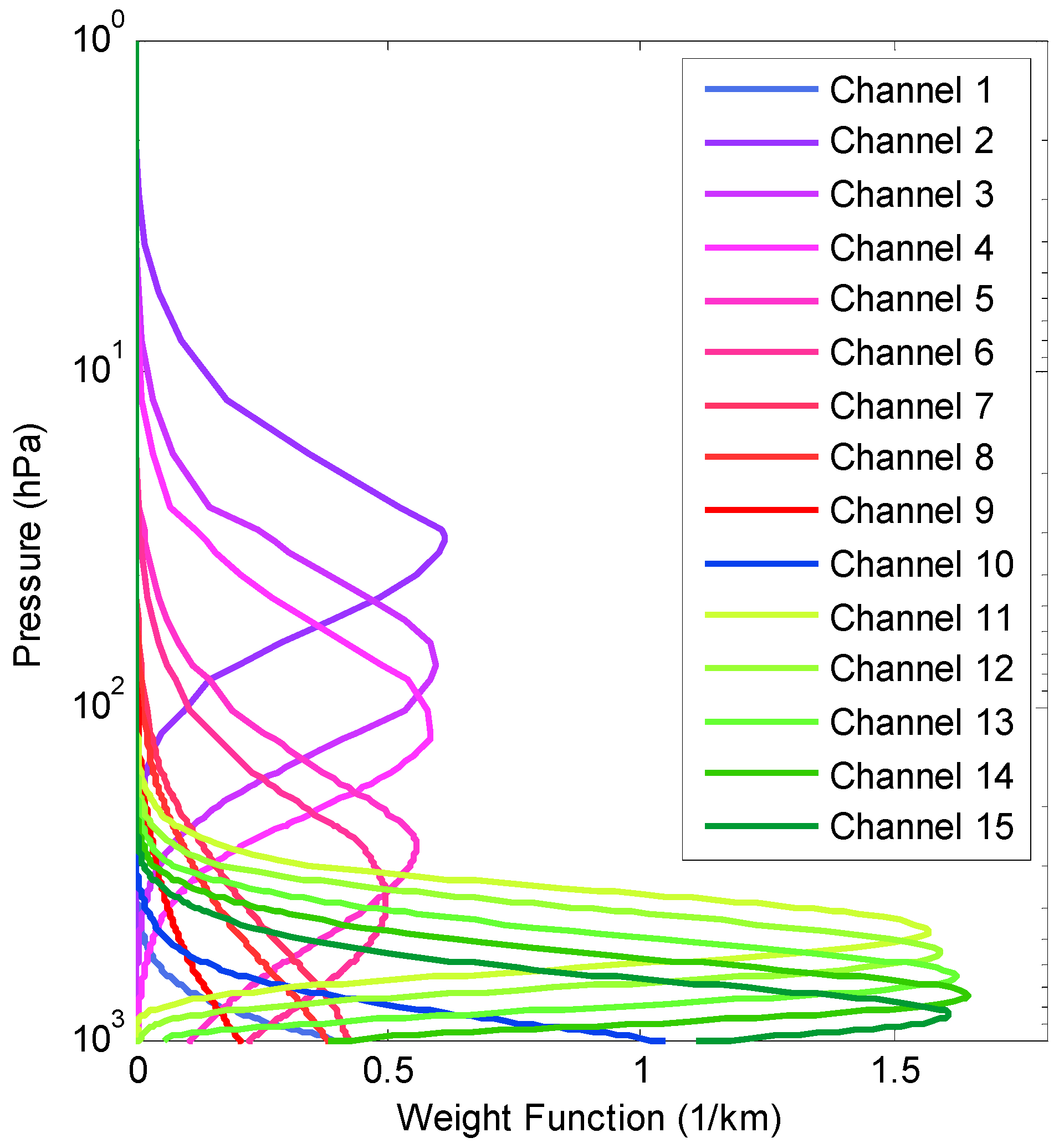
2. Description of MWHTS Instruments’ Characteristics

On 23 September 2013, the FY-3C satellite was successfully launched into a circular, near-polar, morning-configured (1005 Local Time (LT)) orbit with an altitude of 836 km above the Earth and an inclination angle of 98.75° to the Equator. MWHTS onboard FY-3C is a total power radiometer and has a cross-track scanning geometry within ±53.35° with respect to the nadir direction. MWHTS completes one scan every 2.66 s, and its swath is 2645 km, giving a nominal field of view (FOV) of 16 km at nadir. Each scan line has 98 FOVs together with a view of cold space and the onboard warm calibration target used to perform a two-point radiometric calibration [28]. MWHTS has 15 channels with eight temperature sounding channels for measuring temperature from the surface to the upper atmosphere, five humidity sounding channels for measuring water vapor and liquid precipitation from the surface to about 300 hPa and two window channels for providing information on the surface characteristics.

Table 1. MWHTS channel characteristics. WF, weighting function.

Channel	Frequency (GHz)	Polarization Angle	Bandwidth (MHz)	Peak WF (hPa)	In-Flight Sensitivity (K)
1	89	${90}^{°}-\theta$	1500	Window	0.23
2	118.75 ± 0.08	$\theta$	20	30	1.62
3	118.75 ± 0.2	$\theta$	100	50	0.75
4	118.75 ± 0.3	$\theta$	165	100	0.59
5	118.75 ± 0.8	$\theta$	200	250	0.65
6	118.75 ± 1.1	$\theta$	200	350	0.52
7	118.75 ± 2.5	$\theta$	200	Surface	0.49
8	118.75 ± 3.0	$\theta$	1000	Surface	0.27
9	118.75 ± 5.0	$\theta$	2000	Surface	0.27
10	150	${90}^{°}-\theta$	1500	Window	0.34
11	183.31 ± 1	$\theta$	500	300	0.47
12	183.31 ± 1.8	$\theta$	700	400	0.34
13	183.31 ± 3	$\theta$	1000	500	0.3
14	183.31 ± 4.5	$\theta$	2000	700	0.22
15	183.31 ± 7	$\theta$	2000	800	0.27

lists some of the channel characteristics of the FY-3C/MWHTS, including channel frequency, polarization angle, bandwidth, sensitivity of channel measured in flight and peak weighting function (WF) height, where the polarization angle is defined as the angle from horizontal polarization and $\theta$ is the scan angle from nadir.

Figure 1 displays the WF distributions for 15 channels of MWHTS calculated from a standard U.S. atmospheric profile at nadir by Millimeter-wave Propagation Model (MPM)-93 [29]. The WFs indicate the relative contribution of each atmospheric layer to the observations. For a given instrument channel and atmosphere state, the peak WF height increases with increasing zenith angle, since the optical path length sounded by the satellite increases with the instrument scan angles [30]. It is seen that MWHTS Channels 1–9 measure the atmospheric temperature from the surface to 30 hPa, mainly in the stratosphere. MWHTS Channels 10–15 measure the humidity in the troposphere. The WFs for MWHTS Channels 7–9 with frequencies in the far wing region of the 118.75-GHz oxygen absorption line and MWHTS Channels 1, 10 with frequencies near the atmospheric absorption window have their maximum closer to the surface. These channels are affected by the radiation from both the surface and the boundary layer and can be used to obtain Earth’s surface information.

In our study, Level 1b MWHTS brightness temperatures, obtained from the National Satellite Meteorological Center (http://www.nsmc.cma.gov.cn/NSMC/HOME/Index.html), are used. The MWHTS instrument is calibrated through a two-point calibration algorithm. The Level 1b MWHTS brightness temperatures are converted from MWHTS calibration data, including the radiometric counts from the cold space and warm target, the warm target temperature and instrument temperature. These calibration data are converted to brightness temperature using non-linear correction where the nonlinear coefficient is derived from the prelaunch thermal vacuum data, cross-polarization correction and correction of antenna spill-over effects. Before these brightness temperatures are used in quantitative application, such as data assimilation, atmospheric parameters retrieval and climate research, Guo et al. [5] have carried out the on-orbit calibration status and validation tests for the MWHTS product. The MWHTS post-launch instrument performance was evaluated during the first three months on-orbit. They used three methods to validate MWHTS measurements: vicarious calibration using site calibration test, cross-calibration with the products of the Advanced Technology Microwave Sounder (ATMS) at the simultaneous nadir overpass (SNO) and statistical characteristics analysis of the differences between observations and simulations by the Community Radiative Transfer Model (CRTM) in clear sky (i.e., Observation minus Background simulation (O-B)).

Table 2. The calibration results of MWHTS measurements [5].

Channel	Site Calibration Test	Cross Comparison		O-B
	Mean Error (K)	Mean Deviation (K)	Standard Deviation (K)	Mean Deviation (K)	Standard Deviation (K)
1	−1.18	2.08	1.26	−2.97	4.03
2	−0.6	-	-	−0.93	0.43
3	−0.71	-	-	−0.02	0.23
4	−1.21	-	-	−1.98	0.29
5	−1.19	-	-	0.28	0.27
6	−1.25	-	-	−0.34	0.48
7	0.01	-	-	0.78	1.8
8	0.01	-	-	0.8	2.26
9	0.89	-	-	3.94	3.6
10	−0.45	8.14	4.31	−4.32	3.06
11	−0.89	0.27	0.95	3.97	1.36
12	−1.15	0.85	0.82	1.74	1.47
13	0.78	−2.2	0.86	3.03	1.7
14	3.23	−3.94	0.95	3.18	2.08
15	−1.7	0.71	0.94	−1.21	2.39

lists the validation results of these three methods. The post launch site calibration results show that the brightness temperature bias in every channel except 14 is less than 1.3 K. The cross comparison with ATMS observations show that the standard deviations for humidity channels are less than 1 K. Furthermore, O-B validation results show that the differences between the observation and simulations for Channels 2–6 is less than 0.5 K, and the other channels are similar to that for corresponding ATMS channels. For a detailed description of the on-orbit calibration status of the MWHTS, see Guo et al. [5]. In addition, an evaluation of the quality of MWHTS measurements at ECMWF has been carried out by Lawrence et al. [31]. The evaluated results show that the quality of MWHTS observations of the 183-GHz channels is good, and the 118-GHz channels have global biases similar to temperature sounding channels on AMSU-A and ATMS in most cases. For a detailed description of the evaluation of the MWHTS observations, see Lawrence et al. [31].

3. Forward Model and Bias Correction

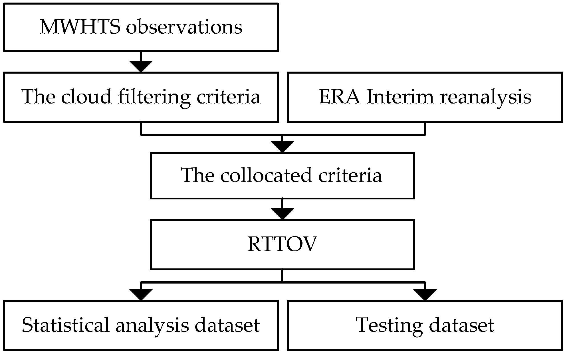
3.1. Forward Model Simulations

Emission, absorption and scattering of the radiation at microwave frequencies by the atmospheric constituents are the physical basis for measuring the atmospheric parameters, such as temperature or humidity. The radiation at the top of the atmosphere measured by a radiometer onboard the satellite can be simulated by a radiative transfer model [32]. In the process of physical retrieval, it is necessary to compare observed and simulated measurements, and the radiative transfer model is an essential part of the physical retrieval algorithm. In this study, the fast radiative transfer model RTTOV (Radiative Transfer for Television and Infrared Observation Satellite Operational Vertical Sounder), Version 11.2, developed by the European Center for Medium-Range Weather Forecast (ECMWF), is used to simulate MWHTS brightness temperatures. Because the surface emissivity has a serious impact on the microwave upwelling radiation, it must be taken into account in radiative transfer simulations [33]. For MWHTS, the surface emissivity affects the measurements of the two window Channels 1, 10, temperature sounding Channels 7–9 and water vapor sounding Channel 15, whose peak WF heights are closer to the surface. In RTTOV [34], over ocean, the surface emissivities are computed by the Faste Emissivity (FASTEM)-5 model [34], over land, a Tool to Estimate Land-Surface Emissivities at Microwave frequencies (TELSEM) emissivity atlas is used [35].

ERA-Interim produced by a data assimilation system, including a four-dimensional variational analysis with a 12-h analysis window, which assimilates many sounding measurements, including radiosondes and in situ sounders, is a reanalysis of the global atmosphere at ECMWF and will be used as inputs to RTTOV to simulate MWHTS observations in our study. For a detailed documentation of the ERA-Interim Archive, see Berrisford et al. [36]. This dataset with a horizontal resolution of 1° × 1° and a temporal resolution of 6 h (i.e., with data available at 0000 UTC, 0600 UTC, 1200 UTC and 1800 UTC) is selected in this work. The profile parameters have a total of 37 pressure levels unevenly spaced from 1000–1 hPa. The profiles of temperature, humidity, cloud liquid water and the surface parameters, including surface pressure, 10-m wind speed, 2-m dew point temperature, 2-m temperature and skin temperature are used as inputs to RTTOV. Due to the lack of accurate information about cloud ice and rain parameters in the ERA-Interim, simulations are carried out by the emission-based model neglecting the scatterings of clouds and precipitation in RTTOV. Ice and snow emissivity are not well characterized in the RTTOV [32], which can strongly contribute to the uncertainty in the simulations. Thus, only ERA-Interim data covering the geographic area (180° W–180° E, 60° S–60° N), where there is an ice-free surface, are utilized.

In order to remove the systematic biases in MWHTS observations, we construct a matchup file, containing the time and space collocated MWHTS observations, simulations from RTTOV and the ERA-Interim reanalysis dataset, to compare simulated and observed measurements. It is worth noting that simulations from RTTOV do not take scattering from clouds and precipitation into account; thus, it is necessary to filter out the MWHTS observations in convective weather. In our study, we use the cloud filtering method developed by Buehler [37] where the term cloud is referred to thick clouds or/and rain. Buehler et al. use the measurements at 183.31 ± 1.00 GHz and the difference of measurements at 183.31 ± 1.00 GHz and 183.31 ± 3.00 GHz to create a threshold to filter out the cloud- and precipitation-affected observations. For a detailed description of the cloud filtering methodology, see Buehler et al. and Burns et al. [37,38,39,40]. For MWHTS, the criteria of cloud filtering are that the brightness temperature difference between Channel 11 and Channel 13 is greater than zero and the brightness temperature of Channel 11 is greater than 240.6 K. The criteria for collocating MWHTS observations with ERA-Interim data are that the time difference between ERA-Interim reanalysis data and MWHTS observations is less than 0.5 h and the absolute distance between the position (latitude and longitude) of ERA-Interim reanalysis data and MWHTS observations is less the 0.5°. Based on the cloud filtering criteria and the collocated criteria, two collocated datasets both including the collocated MWHTS observations, simulations from RTTOV and ERA-Interim reanalysis data have been generated. One is the statistical analysis dataset with 254,612 collocated samples over land and 1,393,744 collocated samples over ocean from 1 February–31 May 2014, and it is used to analyze the bias characterization of MWHTS and train the statistical algorithms. The other is the testing dataset with 67,652 collocated samples over land and 345,039 collocated samples over ocean from 1–30 June 2014, and it is used to evaluate the algorithm performance. The overall MWHTS processing procedures implemented in our study are summarized in Figure 2.

3.2. Bias Correction

For FY-3C/MWHTS measurements, the bias can be put into two categories: scan bias, which changes with the scan angle of the instruments, and air-mass bias, which tends to vary with the air mass and surface characteristics of the Earth. In our study, the bias correction scheme is a two-step process: scan correction and air-mass correction. The bias correction can be carried out by either adjusting the satellite measurements or the simulations [21]. In general, the satellite measurements are adjusted, in order to avoid bias correction at each iteration in the physical retrieval procedure.

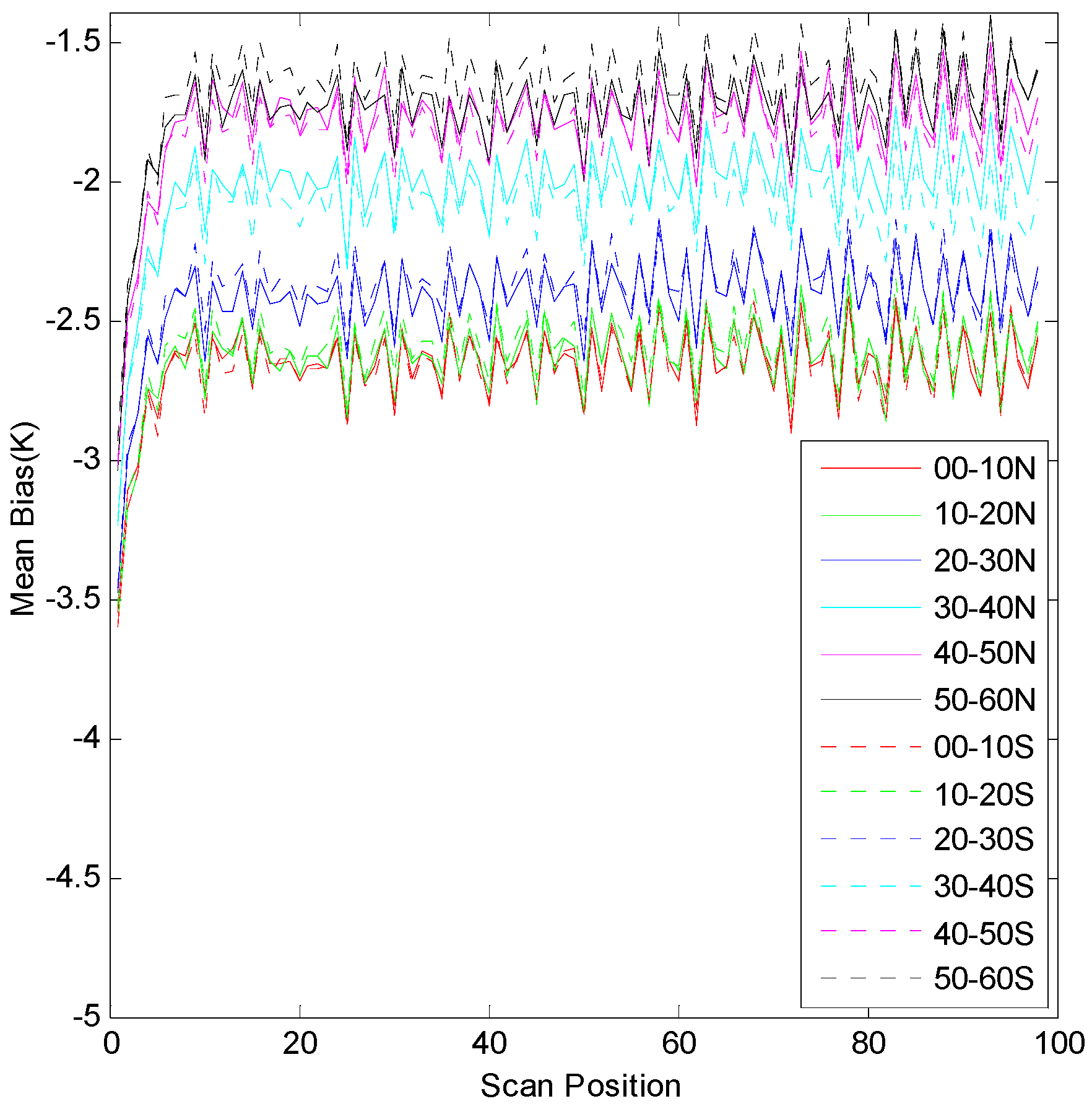
3.2.1. Scan Correction

Though the simulations from RTTOV have taken the scan angle of the instrument into account, which scans in a cross-track manner, residual biases vary with scan positions obviously in the MWHTS measurements, and the biases display noticeable variations in space. Dividing the statistical analysis dataset according to the latitude band, in this case every 10°, we calculate the mean bias between the observed and simulated values. Taking MWHTS Channel 4 for example, Figure 3 shows the distribution of the mean bias by latitude band at 98 scan positions. It can be seen that the biases vary significantly with scan positions, particularly at the first five scan angles. In addition, the biases at different latitude bands are more or less different, and the maximum of the biases’ differences is about 2 K. It is worth noting that there is a dip in bias in the first five scan positions for most MWHTS channels (figure omitted). This probably means that there is contamination at the start scan positions. The actual sources of MWHTS scanning biases may be a combination of some factors, such as the nonlinear correction in the calibration algorithm, the solar contamination on MWHTS onboard the calibration target, center frequency drift, and so on. This requires further research on the root cause analysis.

The scan correction can be divided into 12 latitude bands of 10° of longitude. However, correction coefficients across latitude bands may not be continuous; thus, some smoothing is required. In our study, a simple smoothing approach is carried out to generate a smooth transition between latitude bands as described by Harris et al. [25]. The smoothing is given by:

$$d_j^{\prime }(\varphi ,\theta )=\frac{1}{4}{d}_j(\varphi -1,\theta )+\frac{1}{2}{d}_j(\varphi ,\theta )+\frac{1}{4}{d}_j(\varphi +1,\theta )$$

(1)

where $d$ is mean bias, $\theta$ is the scan angle, $\varphi$ is the latitude band and $j$ is the index of the channel. $d_j(\varphi ,\theta )$ are averaged by the sampling method.

3.2.2. Air-Mass Correction

Bias in the radiative transfer model, because of errors in the physics or spectroscopy, or from imprecise modeling of the atmospheric process, is related to the atmospheric state sounding by the satellite. Removing this bias in physical terms is difficult, in generally, predicting it using a statistical method with bias predictors is preferred. In order to identify the air mass, which can provide a good representation of the atmospheric state, MWHTS observation bias/temperature and bias/humidity correlations, which can be used to study which combinations of atmospheric variables could be taken as bias predictors, are calculated at each pressure level using the statistical analysis dataset compiled in Section 3.1. These correlations are shown in Figure 4. For temperature, it can be seen that there is a correlation between MWHTS brightness temperature bias and the layer 1000–200 hPa, 200–50 hPa and 20–1 hPa for Channels 2–5 and Channels 11–14, but the correlation for Channels 6–10 is very weak. The humidity correlations are displayed for most of the channels in the layer 1000–100 hPa, shown as Figure 4b. In addition, there is a high correlation between the surface temperature and Channel 4. However, it is surprising that, for bias/temperature correlations, the temperature sounding Channels 6–9 show little correlation; for bias/humidity correlations, the humidity sounding channels show weaker correlation than most of the temperature sounding channels; and window Channels 1 and 10, which sense the surface, do not show high correlation with the surface. It is important to realize that we are talking about the bias, not the brightness temperatures themselves. It is not necessary to follow the weight functions shown in Figure 1, that is if a channel senses a given atmosphere layer, the bias will depend on this layer. However, the bias may be caused by another layer, because of correlations present in different layers [25].

As a result of this correlation analysis, we can find that a certain correlation exists between the bias and air mass, but it is not significant, especially in Channels 6–9 for bias/temperature. In order to represent the relationship between the bias and air mass, we consider two kinds of statistical regression methods: linear regression methods and nonlinear regression methods. For the linear regression methods, we select the multiple linear regression model, which is widely used in the bias correction in the operational physical retrieval system and the radiances’ assimilation system. For the nonlinear regression methods, in recent years, many regression models have been introduced to the field of atmosphere remote sensing, such as artificial neural networks, kernel-based regression, particle swarm optimization, support vector machine, and so on. Considering the computational cost, the nonlinear mapping ability and the nonlinear problem solved in our study, we select the neural networks. Therefore, we develop two correction methods: air-mass LRC and NNC, representing the linear and nonlinear relationship between MWHTS observation bias and air mass, respectively.

• LRC method:

Assuming a linear relationship between the brightness temperature bias and the air mass, the LRC method uses a set of bias predictors to predict the bias through the following equation [25]:

$$Z_j={\displaystyle \sum _{i=1}^n{A}_{ji}{X}_i}+C_j$$

(2)

where $j$ is the index of channel, $X_i(i=1,\dots ,n)$ is the bias predictors and $A_{ji}$ and $C_j$ are the coefficients, which are computed by carrying out a least-squares fit on the data samples containing the brightness temperature bias and air mass.

For the bias predictors $X_i$, after some testing, the best combination of predictors for the MWHTS would be: 1000–200 hPa thickness, 200–50 hPa thickness, 20–1 hPa thickness, surface skin temperature and column water vapor. In our study, $X_i$ is constructed using the temperature profiles, humidity profiles and surface skin temperature in the statistical analysis dataset compiled in Section 3.1. $X_i$ and the corresponding differences of observations and simulations are used to calculate the coefficients $A_{ji}$ and $C_j$ in this linear regression algorithm.

• NNC method:

In recent years, neural networks have been widely used in the retrieval of atmospheric geophysical parameters using remote sensing data, as NNs can be used to learn and compute functions for which the analytical relationships between inputs and outputs are complex (e.g., highly nonlinear) [11]. In our study, we focus on BP NNs, which are based on the error back propagation learning algorithm proposed by Rumelhart et al. in 1986, due to their strongly nonlinear mapping ability [41]. Following the vast majority of publications on applying NNs to the atmospheric remote sensing and considering the nonlinear problem of this work, we choose a three-layer networks. The schematic diagram of the three-layer BP NNs containing one hidden layer is shown in Figure 5. The input layer in which no computation is carried out has L nodes representing the length of the input vector $\mathit{X}$. Then, each node is connected to all M nodes of the hidden layer. Each node in the hidden layer performs a nonlinear computation and is connected to each node of the output layer. The output vector $\mathit{Z}$ containing N values is generated by a weighted sum over all of the output vector $\mathit{Y}$ of the hidden layer. Readers interested in additional details on initialization, training, optimization and other advanced topics can refer to [41,42].

In our study, the differences of observations and simulations in the statistical analysis dataset in Section 3.1 are taken as the output vector of the pairs input/output vector, and the corresponding temperature profiles, humidity profiles and skin temperatures are taken as the input vector of the pairs input/output vector (i.e., bias predictors); thus, the length L of the input vector $\mathit{X}$ is 74, and the length N of the output vector $\mathit{Z}$ is 15 in the BP NNs. The steepest descent method is selected in the training phase. Based on many tests, the hidden layer with 30 hidden nodes was found to be best in our study. The connection weights and bias are determined through the training using 90% of the pairs input/output vector; the other 10% of pairs are used for validation and stopping the training.

Finally, based on the above analysis, we can get the corrected brightness temperatures:

$${O^{*}}_j(\varphi ,\theta )=O_j(\varphi ,\theta )-d_j^{\prime }(\varphi ,\theta )-Z_j(\varphi ,\theta )$$

(3)

where ${O^{*}}_j$ is the corrected brightness temperatures in channel j and $O$ is the brightness temperatures without bias correction. In order to evaluate the effects of corrected brightness temperatures on the retrieval accuracy of atmospheric temperature and humidity profiles, we will build a physical retrieval system based on one-dimensional variational algorithm for MWHTS measurements.

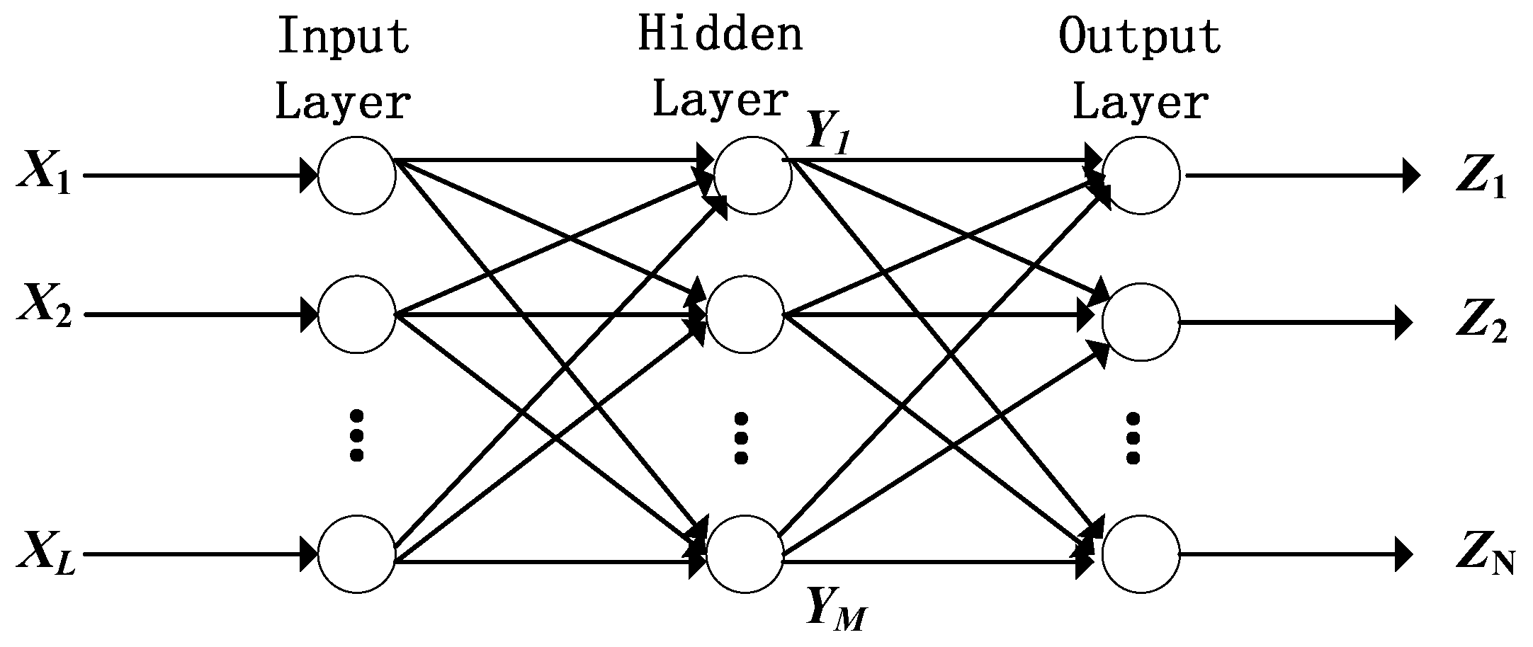
4. Retrieval System for MWHTS

The retrieval system for MWHTS is based on the one-dimensional variational algorithm, which is generally labeled under the general term of physical retrieval. The one-dimensional variational algorithm mainly includes two parts: one is the radiative transfer model for brightness temperature simulations; the other is the minimization of the following cost function:

$$J=\frac{1}{2}{(x-x^b)}^{\mathrm{T}}{\mathit{B}}^{-1}(x-x^b)+\frac{1}{2}{[H(x)-\mathit{I}]}^{\mathrm{T}}{\mathit{R}}^{-1}[H(x)-\mathit{I}]$$

(4)

The cost function is the basis of the one-dimensional variational algorithm; its purpose is weighting the relative contribution of background information and satellite observations. In Equation (4), $x^b$ is the background state variable, and $\mathit{B}$ is the background covariance matrix. $\mathit{R}$ is the sum of the covariance error in the brightness temperature simulations and the sensor noise. $\mathrm{T}$ represents the matrix transpose. $H$ is the forward operator that simulates the satellite observations at the atmospheric state variable $x$. $\mathit{I}$ is the observations. Assuming the errors in the observations and the background information are neither biased nor correlated, Gaussian distributions, and assuming that there is a local linearity around $x$, the minimization of the cost function can be solved by:

$$\frac{\partial J}{\partial x}=0$$

(5)

This results in the solution of $x$ [43]:

$$x_{n+1}=x^b+\mathit{B}{\mathit{H}}^{\mathrm{T}}(x_n){[\mathit{H}(x_n)\mathit{B}{\mathit{H}}^{\mathrm{T}}(x_n)+\mathit{R}]}^{-1}[\mathit{I}-H(X)-(x^b-x_n)]$$

(6)

where $\mathit{H}$ is the tangent linear function of $H$ at point $x$. $n$ is the iteration index. As we can see from Equation (6), the final solution $x_{n+1}$ is affected by the a priori information, including the background covariance matrix $\mathit{B}$, the background state variable $x^b$, the first guess, the bias $\mathit{I}-H(X)$ between observation and simulation, and the covariance matrix $\mathit{R}$.

Due to determining the atmospheric state variable $x$ from satellite observations being an underdetermined and ill-conditioned problem, it is important to use a source of a priori information to constrain the retrievals in the iteration in Equation (6) to get physically-realistic solutions. In our study, we use the atmospheric temperature and humidity profiles from ERA-Interim reanalysis described in Section 3.1, but the time range is from 1 January–30 December 2013, to generate background covariance matrix $\mathit{B}$. The formula is given by [44]:

$${\sigma }_{ij}^2=\frac{1}{N}{\displaystyle \sum _{i=1}^N{\displaystyle \sum _{j=1}^N(x_i-{\overline{x}}_i)}}\times (x_j-{\overline{x}}_j)$$

(7)

where ${\sigma }^2$ is an element in the covariance matrix $\mathit{B}$ and $i$ and $j$ represent the row and column, respectively. $N$ is the number of atmospheric temperature and humidity profiles used. We take the mean of the atmospheric temperature and humidity profiles used in Equation (7) as the background state variable $x^b$ in our retrieval system. $x_1$ in Equation (6) obtained from NWP model outputs is the first guess; the National Centers for Environmental Prediction (NCEP) Climate Forecast System (CFS) 6-h forecasts are used. The details of NCEP CFS are available in Saha et al. [45]. The horizontal and temporal resolution of this dataset is the same as that of ERA-Interim reanalysis and the collocated criteria with MWHTS measurements described in Section 3.1.

For the bias $\mathit{I}-H(X)$, the LRC and NNC methods proposed in Section 3.2 are used to adjust the observed brightness temperatures. After removing biases in the observations, the biases between the observations and the simulations and the sensitivities of MWHTS measured in flight (see Table 1), which are often considered as the instrument channel noise, are used to compute the error covariance matrix $\mathit{R}$ [46]. Assuming that the measurements in one channel are not related to those in the others, the diagonal elements of $\mathit{R}$ are used and given by [21]:

$$r^2=f^2+e^2.$$

(8)

where $r$ is the square roots of the diagonal elements of $\mathit{R}$, $f$ is the instrument channel noise and $e$ is the forward model error. It is worth noting that different correction methods often correspond to different error covariance matrixes.

The convergence criterion adopted in our retrieval system is:

$$\frac{\left|J_{n+1}-J_n\right|}{J_n}<0.01.$$

(9)

This mathematically means that the iteration is stopped if the relative difference of the cost function within two iterations is less than 0.01. Additionally, the maximum of 10 iterations is set. If the iterative times reach 10, the retrieval is set to the first guess. In addition, if the residuals between the measurements and those simulated by RTTOV from the first guess in any channel are greater than 20 K, then the measurements are abandoned. This is carried out for retrieval quality control.

5. Results

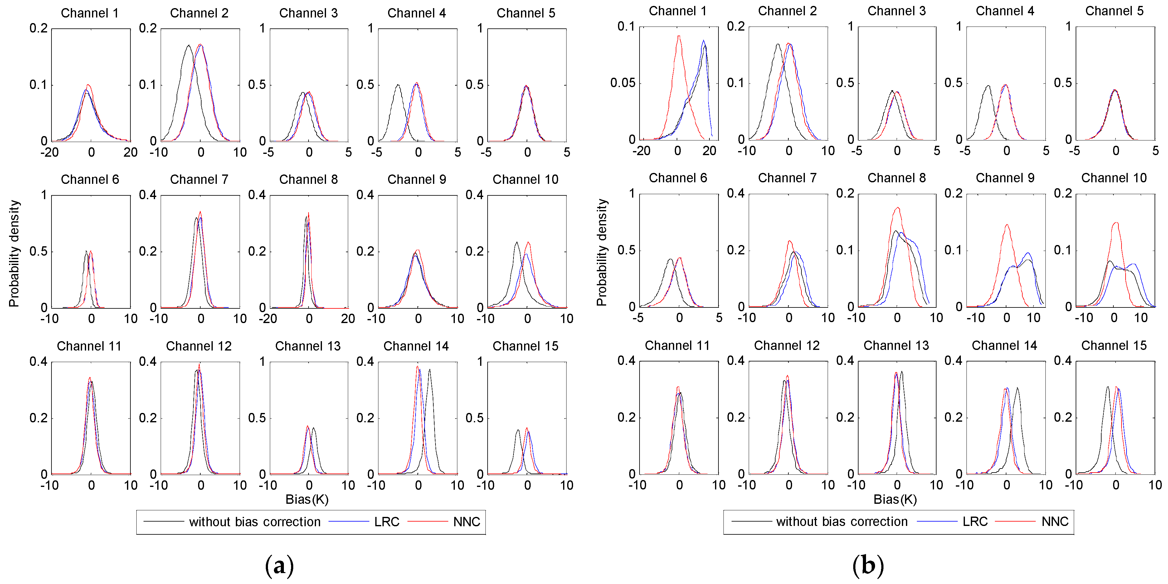
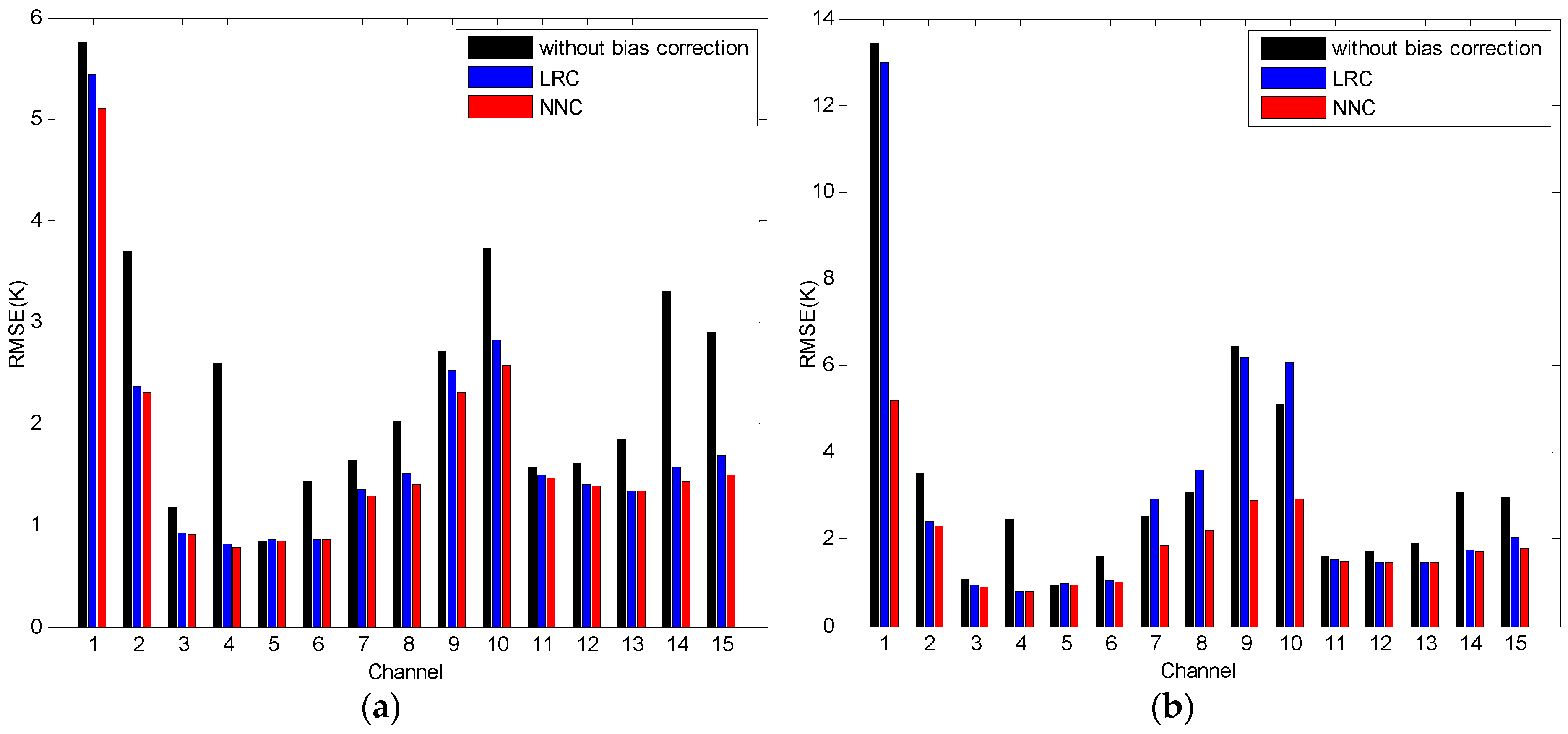
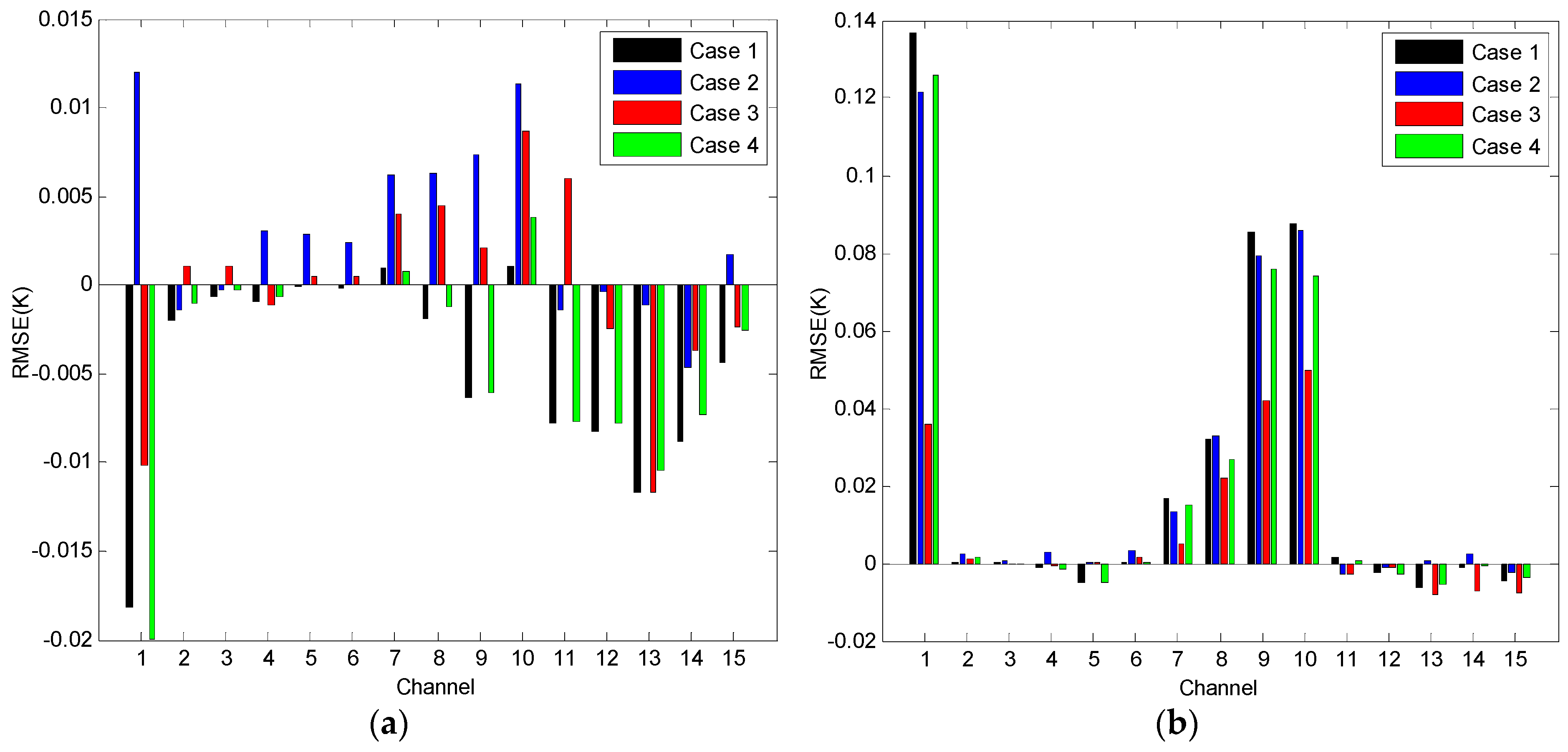
5.1. Bias Correction Results

The LRC and NNC methods are applied to MWHTS observations in the testing dataset in Section 3.1, with the bias predictors generated by the corresponding first guess used in the retrieval system built in Section 4. Figure 6 shows the probability density distribution of brightness temperature biases for MWHTS Channels 1–15 against the simulated brightness temperatures. For the MWHTS observations over ocean, the mean biases in Channels 1–4, 6–8, 10 and 13–15 before bias correction are large, but have been significantly reduced and are close to zero after both LRC and NNC. In addition, the probability density distribution of brightness temperature biases is more similar to a Gaussian distribution than that before bias correction. These two bias correction methods can get the desired correction results. For the MWHTS observations over land, the biases between brightness temperatures and simulated brightness temperatures in Channels 2–7 and 11–15 can be effectively corrected by these two correction methods, and the effect of correction is about the same as that over ocean. However, the biases’ correction in the other channels shows different behaviors when using different correction methods. LRC cannot correct the biases and improve its probability density distribution to make it obey a Gaussian distribution; thus, it will fail in the physical retrieval system. However, the correction results by the NNC method are satisfied. The two correction methods show different behaviors over ocean and land, which may be mainly caused by the surface emissivity. The sea surface emissivity can be calculated accurately by the FASTEM-5 model; but, due to greater variations in surface characteristics, the calculation of the land surface emissivity is complicated, and the accuracy is always lower than that of sea surface emissivity. In addition, the land surface has higher emissivity, which causes the radiation from the surface and the atmosphere close to the surface to be mixed. For Channels 1 and 8–10, which are sensitive to the surface, it is difficult to distinguish whether the contribution is from the land or atmosphere. This leads to the relations of the atmospheric parameters and the biases between observations and simulations to be much more complicated. Due to the strong nonlinearity mapping ability of neural networks, NNC can represent these relations well and get better correction results than LRC.

In order to quantitatively evaluate the performance of these two bias correction methods further, the RMSE is used. The RMSE of the bias before and after bias correction is shown in Figure 7. It can be seen that the RMSE of bias without bias correction is large over both ocean and land, especially in Channels 1 and 8–10, which are sensitive to the surface and the atmosphere close to the surface. Over ocean, the RMSEs of bias in all of the channels corrected by the two correction approaches decrease obviously; the correction performance of NNC is better than that of LRC. However, over land, as expected, the correction performance of bias in Channels 1 and 8–10 corrected by LRC is very poor, the RMSE of bias being even larger than that without bias correction. The RMSEs of bias in temperature sounding Channels 3–7 and water vapor sounding Channels 11–15 are less than those in Channels 1 and 8–10. The RMSEs are within 1.5 K over both ocean and land, and NNC can obtain better correction performance. However, the RMSE of bias in Channel 2 is still very large, though it has reduced significantly using the correction methods. This may be related to the accuracy of the atmospheric temperature profiles in the upper atmosphere.

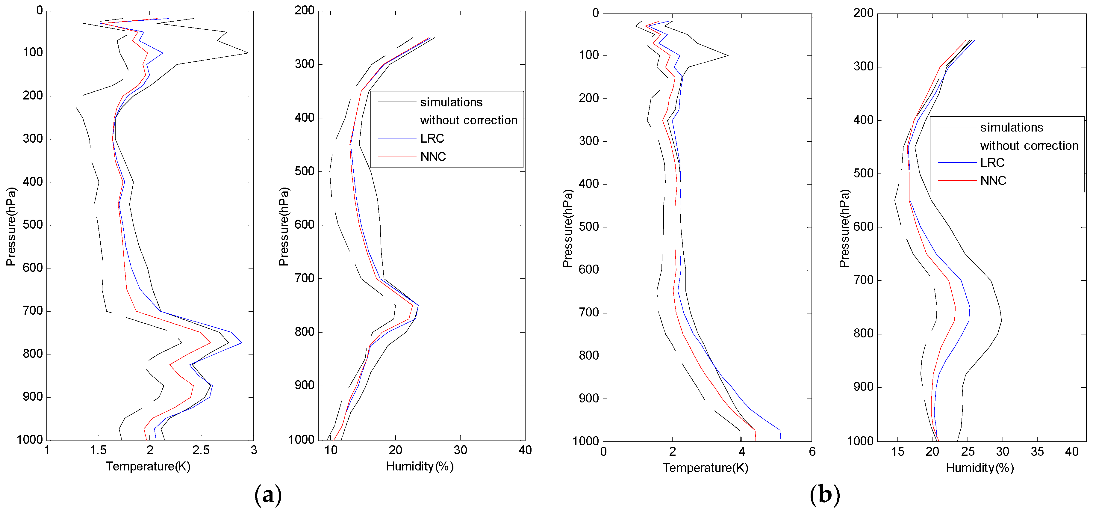
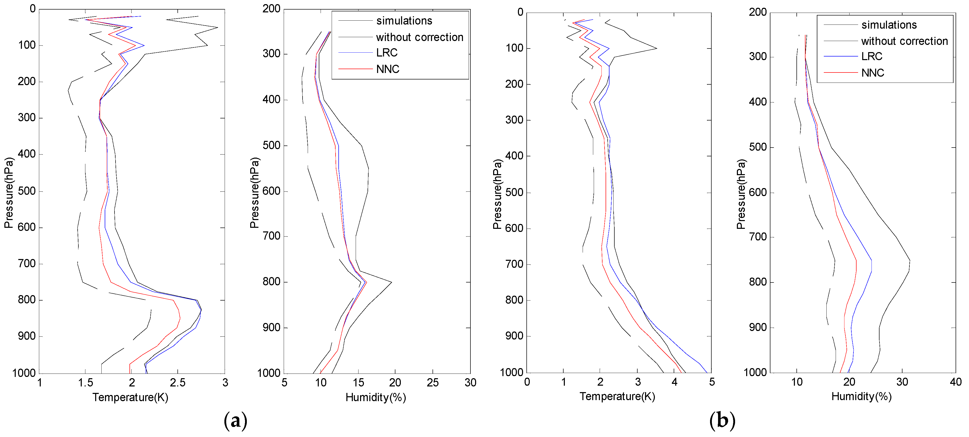
5.2. Results for MWHTS Retrievals

The inversion of MWHTS measurements, including the brightness temperatures with and without bias correction and simulated brightness temperatures in the testing dataset in Section 3.1, into atmospheric temperature and relative humidity profiles was carried out to investigate the influences of the LRC and NNC methods on the inversion accuracy. In our retrieval system, the iterative times are less than five in general. Due to the retrieval quality control, more than 95% and 84% of solutions are obtained convergently over ocean and land, respectively. In our study, RMSE is considered as the standard quantification to validate the retrievals with ECMWF ERA-Interim reanalysis, which is used as the truth. Based on the MWHTS channels’ WF analysis, we validate the retrievals at levels from 1000–20 hPa for temperature and 1000–250 hPa for relative humidity, respectively. Figure 8 shows the RMSE of inversion for the ocean and land cases, respectively. For the retrievals over ocean, the retrieved temperature RMSE using corrected measurements shows that, from 200–20 hPa and 750–450 hPa in which Channels 2–4 and 6 are sensitive, the retrieval accuracy can be increased by 0.9 K. The correction results of these channels are good, as can be seen in Figure 7a. However, the retrieved temperature accuracy using measurements corrected by NNC is better than that of using measurements corrected by LRC at levels from 1000–800 hPa, due to the correction results obtained by NNC outperforming those of LRC. The retrieved temperature accuracy using measurements corrected by LRC is similar to that of measurements without bias correction. Due to the better performance of the NNC method, the retrieved temperature accuracy is closer to the retrieved results using the simulated brightness temperatures. The retrieved humidity RMSE using measurements corrected by the two correction methods is significantly smaller than that of using measurements without bias correction. The retrieval accuracy can be increased by 6.8%. The NNC method works better than the LRC method, as well. Compared with the retrieved results over ocean, we come to the same conclusion that the retrievals using corrected measurements have higher accuracy than those of the measurements without bias correction over land. The retrieval accuracy for temperature and humidity can be increased by 0.8 K and 11%, respectively. However, for the temperature RMSE at levels from 1000–900 hPa where Channels 7–10 are sensitive, the retrieval accuracy of LRC is even lower than that of the measurements without bias correction, due to the biases in Channels 7–10 after bias correction still being high, as can be seen in Figure 7b. It can be found from the retrieved RMSE both over ocean and land that the better bias correction results are, the higher the retrieval accuracy is. The retrieval accuracy using measurements corrected by NNC is most approximate to that of using simulated brightness temperatures. This is means that the NNC method has better performance. In order to further verify the performance of the NNC correction method, NCEP CFS analysis is used as the truth to validate the retrievals. The same horizontal and temporal resolution of this dataset as that of ERA-Interim reanalysis and the collocated criteria with MWHTS measurements described in Section 3.1 is selected. The retrieval validation results are shown in Figure 9. First, the retrieval accuracy is different from that in Figure 8 at some layers of the atmosphere, due to the ECMWF ERA-Interim reanalysis and the NCEP CFS analysis being produced by different radiance assimilation systems. However, the most important one is that we can draw the same conclusion as that in Figure 8. The better the bias correction results are, the higher the retrieval accuracy is. Additionally, the NNC method has better performance than the LRC methods in the inversion of atmospheric temperature and humidity. One important thing to note about these retrieval results is that the temperature and humidity retrieval RMSE using simulated measurements is still large. This is caused by some other factors, such as the background covariance matrix, the background state variable and the first guess. Investigating the effect of these factors on the retrieval accuracy and how to improve the retrievals are beyond the scope of our study in this paper and will be studied in a future publication.

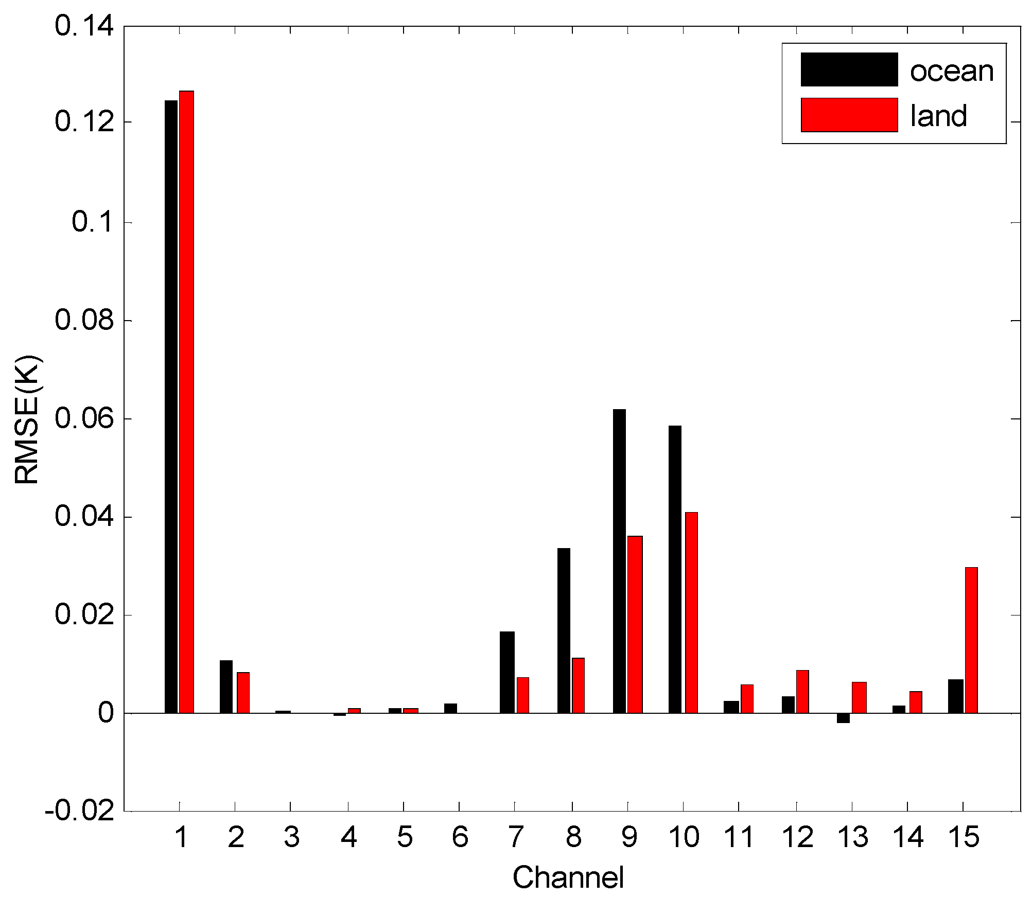
5.3. Evaluation of Algorithm Robustness

From the analyses above, the NNC method can provide excellent performance in the physical process. However, it is necessary to examine the algorithm performance when the atmospheric parameters used to generate the bias predictors fall outside the training dataset of NNs. We should note that, in the training phase of NNC, the atmospheric parameters used to generate the bias predictors come from the ECMWF reanalysis dataset, but in the retrieval system, the first guess used to generate the bias predictors come from the NCEP CFS forecast dataset. Additionally, we have achieved the desired correction results in the retrieval system. There is reason to believe that better correction results can be obtained when the bias predictors are generated by the atmospheric parameters coming from the same data source. However, this cannot be realized in the retrieval system, due to the reanalysis data not being able to be taken as the first guess. Figure 10 shows the difference of the RMSE of bias correction using the first guess as the bias predictors and that of using ERA-Interim reanalysis in the testing dataset as the bias predictors. It can be seen that the differences of the corrected results using atmospheric parameters coming from different data sources are almost equal to zero, except for Channels 1 and 7–10, in which the observations are affected by the surface emissivity. However, the atmospheric parameters used to calculate the surface emissivity may have a large amount of forecast error in the NCEP CFS 6-h forecasts, such as 10-m wind speed. Figure 11 shows the effects of the different corrected results on the retrieval accuracy. The differences are too small to be statistically significant; thus, the correction biases caused by bias predictors using different data sources in our retrieval system have little effect on the retrieval accuracy. These suggest that the performance of the NNC method proposed in our study is fairly robust in the retrieval system.

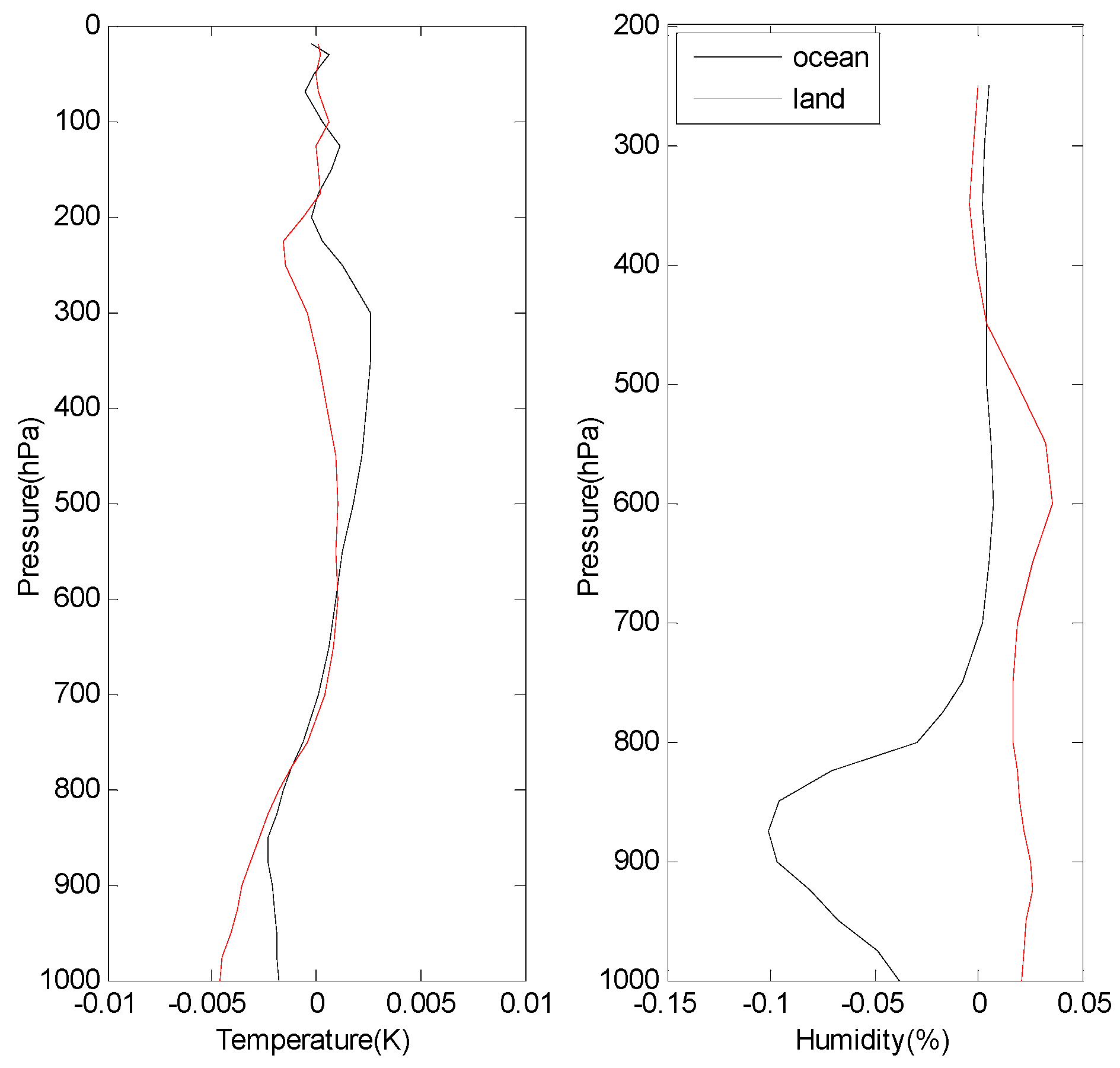
5.4. Evaluation of Algorithm Stability

A well-constructed NN can obtain the same solution, which is not affected by the NN’s initialization represented by the weights and biases used at the start of training. We can assess the stability of the algorithm through examining the solutions returned by NNC with different initialization states. We retrained the NNs of NNC with randomly-initialized weights and biased for four separate times, then applied the NNC method to the same MWHTS observations as that of Section 5.1. Figure 12 shows the differences of the RMSE of bias correction between four bias corrections and the NNC bias correction in Section 5.1. It can be seen that the corrected results obtained by the four cases are similar to those in Section 5.1, both over ocean and land. The differences of the RMSE of bias correction over land are greater than those over ocean obviously, because of being affected by surface emissivity. However, the differences are too small to affect the retrieval accuracy in our inversion system, which is the same as that of Figure 11. These suggest that the NNC method proposed in our study is insensitive to the initialization state.

6. Conclusions

In this work, two air mass correction methods have been proposed: LRC and NNC, representing the linear and nonlinear character between MWHTS measurements and air mass, respectively, to correct the systemic biases between the MWHTS observations and simulations coming from the radiative transfer model in the physical retrieval process. It has been shown that the NNC method obtains the desired correction results and outperforms the LRC method. Incorporating such correction brightness temperatures in the one-dimensional variational system built in this study can obtain higher retrieval accuracies of atmospheric temperature and humidity profiles than those of LRC and those without bias correction. These also suggest that the better the correction results are, the higher the retrieval accuracy in the physical process is. To fully assess the performances of the NNC method, NNC is carried out with bias predictors coming from NCEP CFS forecasts and ECMWF reanalysis, respectively. The results of the comparison suggest that NNC is fairly robust. The sensitivity of NNC to the initialization of the NNs at the start of training shows that NNC is much stabilized.

In conclusion, the NNC method proposed in this paper is promising in the physical retrieval system. Meanwhile, when the NNC method is applied in the statistical retrieval, simulations rather than the actual measurements can be used; thus, the collocated error between the satellite observations and atmospheric variables in time and space can be ignored. Nevertheless, NNC is not suitable in the NWP radiance assimilation system, in which an adaptive bias correction scheme is preferred to distinguish satellite observation bias from the NWP model bias and to prevent the contamination of the observation bias estimates by systemic NWP model errors.

References

1. Ebell, K.; Orlandi, E.; Hünerbein, A.; Löhnert, U.; Crewell, S. Combining ground-based with satellite-based measurements in the atmospheric state retrieval: Assessment of the information content. J. Geophys. Res. 2013, 118, 6940–6956. [Google Scholar] [CrossRef]
2. Ahn, M.H.; Kim, M.J.; Chung, C.Y.; Suh, A.S. Operational implementation of the ATOVS processing procedure in KMA and its validation. Adv. Atmos. Sci. 2003, 20, 398–414. [Google Scholar] [CrossRef]
3. Miao, J.; Kunzi, K.; Heygster, G.; Lachlan-Cope, T.A.; Turner, J. Atmospheric water vapor over Antarctica derived from Special Sensor Microwave/Temperature 2 data. J. Geophys. Res. 2001, 106, 10187–10203. [Google Scholar] [CrossRef]
4. Duck, T.J. A microwave satellite water vapor column retrieval for polar winter conditions. Atmos. Meas. Tech. 2016, 9, 2241–2252. [Google Scholar]
5. Guo, Y.; Lu, N.M.; Qi, C.L.; Gu, S.Y.; Xu, J.M. Calibration and validation of microwave humidity and temperature sounder onboard FY-3C satellite. Chin. J. Geophys. Chin. 2015, 58, 20–31. [Google Scholar]
6. Polyakov, A.; Timofeyev, Y.M.; Virolainen, Y. Comparison of different techniques in atmospheric temperature-humidity sensing from space. Int. J. Remote Sens. 2014, 35, 5899–5912. [Google Scholar]
7. Gohil, B.S.; Gairola, R.M.; Mathur, A.K.; Varma, A.K.; Mahesh, C.; Gangwar, R.K.; Pal, P.K. Algorithms for retrieving geophysical parameters from the MADRAS and SAPHIR sensors of the Megha-Tropiques satellite: Indian scenario. Q. J. R. Meteorol. Soc. 2013, 139, 954–963. [Google Scholar] [CrossRef]
8. Rao, T.N.; Sunilkumar, K.; Jayaraman, A. Validation of humidity profiles obtained from SAPHIR, on-board Megha-Tropiques. Curr. Sci. India 2013, 104, 1635–1642. [Google Scholar]
9. Shi, L. Retrieval of atmospheric temperature profiles from AMSU-A measurements using a neural network approach. J. Atmos. Ocean Technol. 2001, 18, 340–347. [Google Scholar] [CrossRef]
10. Chen, H.; Jin, Y.Q. Data validation of Chinese microwave FY-3A for retrieval of atmospheric temperature and humidity profiles during Phoenix typhoon. Int. J. Remote Sens. 2011, 32, 8541–8554. [Google Scholar] [CrossRef]
11. Blackwell, W.J.; Chen, F.W. Neural Networks in Atmospheric Remote Sensing; Artech House: Norwood, MA, USA, 2009. [Google Scholar]
12. Liu, D.; Lv, C.; Liu, K.; Xie, Y.; Miao, J. Retrieval analysis of atmospheric water vapor for K-band ground-based hyperspectral microwave radiometer. IEEE Trans. Geosci. Remote Sens. 2014, 11, 1835–1839. [Google Scholar]
13. Stähli, O.; Murk, A.; Kämpfer, N.; Mätzler, C.; Eriksson, P. Microwave radiometer to retrieve temperature profiles from the surface to the stratopause. Atmos. Meas. Tech. 2013, 6, 2477–2494. [Google Scholar] [CrossRef]
14. Bleisch, R.; Kämpfer, N.; Haefele, A. Retrieval of troposphere water vapor by using spectra of a 22 GHz radiometer. Atmos. Meas. Tech. 2011, 4, 1891–1903. [Google Scholar] [CrossRef] [Green Version]
15. Weng, F.; Zou, X.; Wang, X.; Yang, S.; Goldberg, M.D. Introduction to Suomi national polar-orbiting partnership advanced technology microwave sounder for numerical weather prediction and tropical cyclone applications. J. Geophys. Res. 2012, 117. [Google Scholar] [CrossRef]
16. Dee, D.P. Bias and data assimilation. Q. J. R. Meteorol. Soc. 2005, 131, 3323–3343. [Google Scholar] [CrossRef]
17. Auligné, T.; McNally, A.P.; Dee, D.P. Adaptive bias correction for satellite data in a numerical weather prediction system. Q. J. R. Meteorol. Soc. 2007, 133, 631–642. [Google Scholar] [CrossRef]
18. Susskind, J.; Rosenfield, J.; Reuter, D. An accurate radiative transfer model for use in the direct physical inversion of HIRS2 and MSU temperature sounding data. J. Geophys. Res. 1983, 88, 8550–8568. [Google Scholar] [CrossRef]
19. Smith, W.L.; Woolf, H.M.; Hayden, C.M.; Schreiner, A.J. The physical retrieval TOVS Export Package. In Proceedings of the Technical Proceedings of the First TOVS Study Conference, Igls, Austria, 29 August–2 September 1983.
20. Weng, F.; Zhao, L.; Ferraro, R.R.; Poe, G.; Li, X.; Grody, N.C. Advanced microwave sounding unit cloud and precipitation algorithms. Radio Sci. 2003, 38. [Google Scholar] [CrossRef]
21. Li, J.; Wolf, W.W.; Menzel, W.P.; Zhang, W.; Huang, H.L.; Achtor, T.H. Global soundings of the atmosphere from ATOVS measurements: The algorithm and validation. J. Appl. Meteorol. 2000, 39, 1248–1268. [Google Scholar] [CrossRef]
22. Kelly, G.A.; Flobert, J.F. Radiance tuning. In Proceedings of the Technical Proceedings of the Fourth TOVS Study Conference, Igls, Austria, 16–22 March 1988.
23. McMillin, L.M.; Crone, L.J.; Crosby, D.S. Adjusting satellite radiances by regression with an orthogonal transformation to a prior estimate. J. Appl. Meteorol. 1989, 28, 969–975. [Google Scholar] [CrossRef]
24. Uddstrom, M. Forward model errors. In Proceedings of the Technical Proceedings of the Sixth TOVS Study Conference, Airlie, VA, USA, 1–6 May 1991.
25. Harris, B.A.; Kelly, G. A satellite radiance-bias correction scheme for data assimilation. Q. J. R. Meteorol. Soc. 2001, 127, 1453–1468. [Google Scholar] [CrossRef]
26. Dee, D.P. Variational bias correction of radiance data in the ECMWF system. In Proceedings of the Workshop on Assimilation of High Spectral Resolution Sounders in NWP, Reading, UK, 28 June–1 July 2004.
27. Dee, D.P.; Uppala, S. Variational bias correction of satellite radiance data in the ERA-Interim reanalysis. Q. J. R. Meteorol. Soc. 2009, 135, 1830–1841. [Google Scholar] [CrossRef]
28. Wu, C.Q.; Ma, G.; Qi, C.L.; Guo, Y.; You, R. Retrieval of Atmospheric and Surface Parameters from VASS/FY-3C Data under Non-Precipitation Condition; SPIE Asia Pacific Remote Sensing; International Society for Optics and Photonics: Beijing, China, 2014. [Google Scholar]
29. Liebe, H.J.; Hufford, G.A.; Cotton, M.G. Propagation modeling of moist air and suspended water/ice particles at frequencies below 1000 GHz. In Proceedings of the AGARD 52nd Specialists Meeting of Electromagnetic Wave Propagation Panel, Palma De Mallorca, Spain, 17–21 May 1993.
30. Karbou, F.; Aires, F.; Prigent, C.; Eymard, L. Potential of Advanced Microwave Sounding Unit-A (AMSU-A) and AMSU-B measurements for atmospheric temperature and humidity profiling over land. J. Geophys. Res. 2005, 110, D07109. [Google Scholar] [CrossRef]
31. Lawrence, H.; Bormann, N.; Lu, Q.; Geer, A.; English, S. An Evaluation of FY-3C MWHTS-2 at ECMWF; EUMETSAT/ECMWF Fellowship Programme Research Report, 37; ECMWF: Reading, UK, 2015. [Google Scholar]
32. Zou, X.; Wang, X.; Weng, F.; Li, G. Assessments of Chinese Fengyun Microwave Temperature Sounder (MWTS) measurements for weather and climate applications. J. Atmos. Ocean. Technol. 2011, 28, 1206–1227. [Google Scholar] [CrossRef]
33. Sivira, R.; Brogniez, H.; Mallet, C.; Oussar, Y. A layer-averaged relative humidity profile retrieval for microwave observations: Design and results for the Megha-Tropiques payload. Atmos. Meas. Tech. 2015, 8, 1055–1071. [Google Scholar] [CrossRef] [Green Version]
34. Saunders, R.; Hocking, J.; Rundle, D.; Rayer, P.; Matricardi, M.; Geer, A.; Lupu, C.; Brunel, P.; Vidot, J. RTTOV-11 Science and Validation Report; NWP-SAF Report; Met Office: Exeter, UK, 2013; pp. 1–62.
35. Aires, F.; Prigent, C.; Bernardo, F.; Jiménez, C.; Saunders, R.; Brunel, P. A Tool to Estimate Land-Surface Emissivities at Microwave frequencies (TELSEM) for use in numerical weather prediction. Q. J. R. Meteorol. Soc. 2011, 137, 690–699. [Google Scholar] [CrossRef] [Green Version]
36. Berrisford, P.; Dee, D.; Poli, P.; Brugge, R.; Fielding, K.; Fuentes, M.; Kallberg, P.; Kobayashi, S.; Uppala, S.; Simmons, A. The ERA-Interim Archive Version 2.0; ERA Report Series 1; European Centre for Medium-Range Weather Forecasts (ECMWF): Reading, UK, 2011. [Google Scholar]
37. Buehler, S.A.; Kuvatov, M.; Sreerekha, T.R.; John, V.O.; Rydberg, B.; Eriksson, P.; Notholt, J. A cloud filtering method for microwave upper tropospheric humidity measurements. Atmos. Chem. Phys. 2007, 7, 5531–5542. [Google Scholar] [CrossRef]
38. Burns, B.A.; Wu, X.; Diak, G.R. Effects of precipitation and cloud ice on brightness temperatures in AMSU moisture channels. IEEE Trans. Geosci. Remote Sens. 1997, 35, 1429–1437. [Google Scholar] [CrossRef]
39. Greenwald, T.J.; Christopher, S.A. Effects of clod clouds on satellite measurements near 183 GHz. J. Geophys. Res. 2002, 107, 4170. [Google Scholar] [CrossRef]
40. Hong, G.; Heygster, G.; Miao, J.; Kunzi, K. Detection of tropical deep convective clouds from AMSU-B water vapor channels measurements. J. Geophys. Res. 2005, 110, D05205. [Google Scholar] [CrossRef]
41. Rumelhart, D.E.; Hinton, G.E.; Williams, R.J. Learning Internal Representations by Error Propagation; Technical Report, DTIC Doument; MIT Press: Cambridge, MA, USA, 1985. [Google Scholar]
42. Yao, Z.G.; Chen, H.B.; Lin, L.F. Retrieving atmospheric temperature profiles from AMSU-A data with neural networks. Adv. Atmos. Sci. 2005, 22, 606–616. [Google Scholar]
43. Liu, Q.; Weng, F. One-dimensional variational retrieval algorithm of temperature, water vapor, and cloud water profiles from advanced microwave sounding unit (AMSU). IEEE Trans. Geosci. Remote Sens. 2005, 43, 1087–1095. [Google Scholar]
44. Boukabara, S.A.; Garrett, K.; Chen, W.; Iturbide-Sanchez, F.; Grassotti, C.; Kongoli, C.; Chen, R.; Liu, Q.; Yan, B.; Weng, F.; et al. MiRS: An all-weather 1DVAR satellite data assimilation and retrieval system. IEEE Trans. Geosci. Remote Sens. 2011, 49, 3249–3272. [Google Scholar] [CrossRef]
45. Saha, S.; Moorthi, S.; Wu, X.; Wang, J.; Nadiga, S.; Tripp, P.; Behringer, D.; Hou, Y.T.; Chuang, H.Y.; Iredell, M.; et al. The NCEP climate forecast system version 2. J. Clim. 2014, 27, 2185–2208. [Google Scholar] [CrossRef]
46. English, S.J. Estimation of temperature and humidity profile information from microwave radiances over different surface types. J. Appl. Meteorol. 1999, 38, 1526–1541. [Google Scholar] [CrossRef]
Figure 1. Weight functions for the 15 channels of FY-3C/MWHTS calculated from the U.S. standard atmospheric profile at nadir, assuming a surface emissivity of 0.6.
Atmosphere 07 00156 g001
Figure 2. The flow chart for the MWHTS observations’ processing procedure.
Atmosphere 07 00156 g002
Figure 3. Scan bias by latitude band, FY-3C/MWHTS Channel 4.
Atmosphere 07 00156 g003
Figure 4. Atmospheric parameters-bias correlations, MWHTS Channels 1–15: (a) temperature bias; (b) humidity bias.
Atmosphere 07 00156 g004
Figure 5. Diagram of the BP neural networks.
Atmosphere 07 00156 g005
Figure 6. Probability density distributions of brightness temperature biases for MWHTS Channels 1–15 against the simulated brightness temperatures. (a) Over ocean; (b) over land. LRC, linear regression correction; NNC, neural network correction.
Atmosphere 07 00156 g006
Figure 7. The RMSE of the biases before and after bias correction for MWHTS Channels 1–15. (a) Over ocean; (b) over land.
Atmosphere 07 00156 g007
Figure 8. Temperature and relative humidity RMSE of retrieval over: (a) ocean; (b) land.
Atmosphere 07 00156 g008
Figure 9. The retrieval RMSE with respect to NCEP Climate Forecast System (CFS) analysis over: (a) ocean; (b) land.
Atmosphere 07 00156 g009
Figure 10. RMSE of bias correction using the first guess as the bias predictors minus the RMSE of bias correction using the ECMWF reanalysis as the bias predictors.
Atmosphere 07 00156 g010
Figure 11. Same as Figure 10, but for retrieval accuracy.
Atmosphere 07 00156 g011
Figure 12. The differences of the RMSE of the bias correction between four bias corrections and the NNC bias correction in Section 5.1. (a) Over ocean; (b) over land.
Atmosphere 07 00156 g012