Article

Evaluation of Optimized WRF Precipitation Forecast over a Complex Topography Region during Flood Season

1
College of Hydrology and Water Resources, Hohai University, Nanjing 210098, China
2
Jiangsu Electric Power Design Institute, Nanjing 211100, China
3
Pearl River Water Resources Commission of the Ministry of Water Resources, Guangzhou 510611, China
*
Author to whom correspondence should be addressed.
Atmosphere 2016, 7(11), 145; https://doi.org/10.3390/atmos7110145
Submission received: 8 October 2016 / Revised: 8 November 2016 / Accepted: 9 November 2016 / Published: 17 November 2016
(This article belongs to the Special Issue WRF Simulations at the Mesoscale: From the Microscale to Macroscale)

Abstract

:
In recent years, the Weather Research and Forecast (WRF) model has been utilized to generate quantitative precipitation forecasts with higher spatial and temporal resolutions. However, factors including horizontal resolution, domain size, and the physical parameterization scheme have a strong impact on the dynamic downscaling ability of the WRF model. In this study, the influence of these factors has been analyzed in precipitation forecasting for the Xijiang Basin, southern China—a region with complex topography. The results indicate that higher horizontal resolutions always result in higher Critical Success Indexes (CSI), but higher biases as well. Meanwhile, the precipitation forecast skills are also influenced by the combination of microphysics parameterization scheme and cumulus convective parameterization scheme. On the basis of these results, an optimized configuration of the WRF model is built in which the horizontal resolution is 10 km, the microphysics parameterization is the Lin scheme, and the cumulus convective parameterization is the Betts–Miller–Janjic scheme. This configuration is then evaluated by simulating the daily weather during the 2013–2014 flood season. The high Critical Success Index scores and low biases at various thresholds and lead times confirm the high accuracy of the optimized WRF model configuration for Xijiang Basin. However, the performance of the WRF model varies from different sub-basins due to the complexity of the mesoscale convective system (MCS) over this region.

1. Introduction

Quantitative precipitation forecast (QPF) plays a significant role in the prevention of natural disasters such as flood and rainstorms [1,2]. Numerical weather forecasts have been commonly used to provide QPF products in recent years [3,4,5]. However, the global numerical weather forecast models can not meet the requirement of high spatial and temporal resolution of a specific region with complicated topography, due to the limitation of computer resources. Many regional numerical weather forecast models—such as the Regional Atmospheric Modeling System (RAMS), the Pennsylvania State University–National Center for Atmospheric Research (PSU/NCAR) mesoscale model (MM5) and the Weather Research and Forecast model (WRF)—have been provided as dynamic downscaling tools to generate higher spatial and temporal resolution QPF products on the basis of global numerical weather forecasts [6,7]. Numerous studies have indicated that regional numerical weather forecast models are more capable of predicting precipitation in complicated topography than global models, as higher resolution helps to reveal local circulations and orographic forcing [8].
However, predicting precipitation in a complex terrain region remains challenging, and the performance of regional model remains to be improved [9]. Although a great range of options have been provided for regional models in order to be flexible to any region in the world, studies have indicated that there is still a need to establish a proper configuration for a given area with complex terrain. Carvalho et al. [10] simulated wind energy in an area of Portugal with complex terrain under different numerical and physical options, and the results indicated that the MM5–Yonsei University–Noah was the most suitable parameterization set for this site, and demonstrated that the increase of domain resolution alone cannot improve the model performance significantly. Zhang et al. [11] also found out that increasing the vertical resolution by the use of the WRF model may not help to predict 2-m temperature and 10-m wind speed in complex terrain. Cheng and Steenburgh [12] suggested that using a more sophisticated land surface model was not able to get a higher forecast skill over the Western United States.
Numerous options, including spatial resolutions, domain size, and microphysics parameterization schemes, always make it difficult to establish a proper dynamic configuration for a given region. However, model characteristics such as land surface model and vertical horizontal resolution may have less influence on precipitation forecast when compared with physical parameterizations. It is more feasible to concentrate on the optimization of several key options. Horizontal resolution is the most important option when setting up a downscaling configuration for regional models. However, the capability of increasing precipitation forecast skill with higher resolution remains to be discussed. The prediction skills of South Asia increased with higher horizontal resolution, while the skills did not enhance to Southeast Asia and oceans [13]. Another aspect that we must take into consideration is the domain size of simulation. Larger domain sizes lead to larger internal variability of model and longer computing time, but a small domain size makes it difficult for regional models to catch sight of large-scale features inherited from the lateral boundary conditions [14]. Dynamic downscaling method was effective only when the domain sizes get relatively smaller, but a calibrated domain size was needed for subdomains [15]. Microphysics and convective parameterization in regional models help to resolve micro-scale weather systems, and play an important role on the distribution and intensity of precipitation forecasts in regions with complex terrain. Haghroosta et al. [16] suggested that we should select suitable options for different variables.
The Xijiang Basin of south China has a complex topography, and rainstorm disasters are frequent due to the influence of monsoon climate and the occurrence of tropical cyclones. Because the QPF of Xijiang Basin still has low accuracy, there is an urgent need to provide QPF products with higher spatial and temporal resolutions. The Weather Research and Forecast (WRF) model has been proved to be an efficient dynamic downscaling tool in recent years [17]. In this paper, horizontal resolution, domain size, and physical parameterization of the WRF model are optimized through sensitivity tests. An optimized dynamic downscaling configuration is established in Xijiang Basin, and the configuration is verified by evaluating precipitation forecast accuracy during the 2013–2014 flood seasons (1st June–31st August).

2. Data and Methodology

2.1. Study Area and Data Sources

The Xijiang Basin is located at 21.31 ° N–26.49 ° N and 102.14 ° E–112.88 ° E, and covers an area of 406,000 km 2 (Figure 1). The region contains the major tributary of the Pearl River, which originates in the Maxiong Mountains of Yunnan Province, southwest China, and flows through the Guizhou, Guangxi, and Guangdong Provinces, before entering the South China Sea through the Pearl River Delta. Elevation in the basin decreases from the northwest (the Yunnan–Guizhou Plateau) to the southeast delta area. The runoff generation mechanism and concentration time under such complex topography are still under investigation. What is more, the complex topography makes it difficult to gather adequate precipitation information, which is essential to flood forecasts. These factors make it challenging to forecast flood events prior to the periods of runoff concentration.
The region is characterized by a subtropical-to-tropical monsoon climate [18]. Mean annual rainfall over the last three decades varied between 900 and 2200 mm (Figure 2). The Beipanjiang (BPJ) and Nanpanjiang (NPJ) sub-basins are situated to the west, where the annual precipitation is between 900 and 1300 mm. The annual precipitation of the Hongshuihe (HSH) and Yujiang (YJ) Basins are relatively higher than those of BPJ and NPJ, but lower than the others, which include Qianjiang–Liujiang (QLJ), Guijiang (GJ), Xunjiang (XUN), and Xijiang (XIJ). The flooding season extends from April to September, during which nearly 72%–88% of the annual runoff is formed. The area of each sub-basin is shown in Table 1.
The Global Forecast System (GFS) forecast data was used as input to the WRF model. Although the GFS model provides various forecast products with different horizontal resolutions, this study mainly focused on the downscaling capability of the WRF model. The resolution of the 0.5 ° × 0.5 ° GFS product is too high to conduct a sensitivity test, while the resolution of the 2.5 ° × 2.5 ° GFS product is too coarse. Thus, the GFS forecast product we used in this study was at a horizontal resolution of 1 ° × 1 ° and had a frequency of 6 h. The model chosen to conduct the simulations was WRF version 3.5 of the Advanced Research (ARW) solver. It represented the current state-of-the-art in mesoscale model development, and was established as a successor to the long-standing MM5 model, sharing much of the same dynamics and model physics. A more detailed description can be found in a previous study [19]. The observed precipitation of the Xijiang Basin was derived from the real-time operational system of daily precipitation analysis over China on a 0.25 ° × 0.25 ° grid, which was merged from over 2400 stations over mainland China and satellite estimates [20].

2.2. Experimental Design of Sensitivity Tests

Seven typical rainstorms (Table 2), formed because of substantial convective systems, were selected from the 2005–2010 Xijiang Basin data.
All simulations were integrated for 24 h. Different horizontal resolutions, domain sizes, and physical parameterizations were used for each case. All other options (such as integration steps and soil level) which were of lesser importance to the simulations were kept the same. All simulations were run on a Lambert conformal projection. The vertical structure of the model included 28 layers covering the whole troposphere, and the model top was at 50 mb. With the exception of the microphysical and convective parameterization schemes, the physical parameterization schemes for all simulations used were: Yonsei University scheme for the boundary layer [21], the Monin–Obukhov scheme for the surface layer [22], Dudhia for shortwave [23], the Rapid Radiative Transfer Model (RRTM) for longwave radiation [24], and the Noah scheme [25] for land surface.

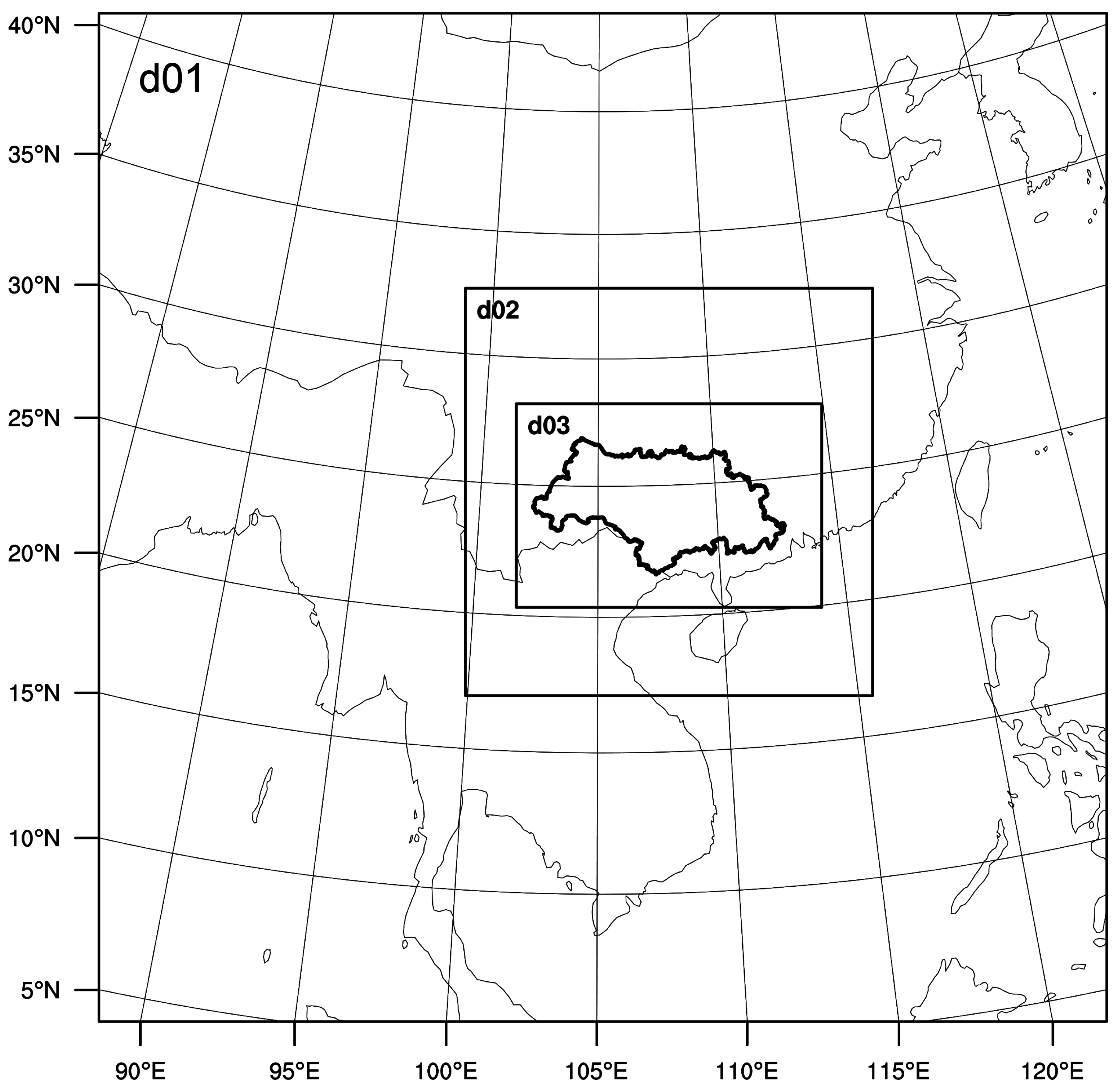
2.2.1. Experimental Design of Horizontal Resolution and Domain Size Sensitivity

For the horizontal resolution sensitivity tests, different nesting strategies were set with different domain sizes (Figure 3 and Table 3). The results of different horizontal resolutions, 45 km (d01), 30 km (d01), 20 km (d01), 15 km (d02), 10 km (d02) and 5 km (d03) were compared to investigate the influence of horizontal resolution and domain size on precipitation forecasts.
Studies have indicated that the numerical forecast models are capable of resolving mesoscale convective systems when the horizontal resolution is higher than 10 km, which means that the utilization of a cumulus convective parameterization scheme at such a high resolution may overestimate the processes of cumulus convections. However, a discussion still exists about whether the high horizontal resolution (<10 km) numerical models are able to resolve the convective processes completely when the scale of cumulus convective processes is lower than 5 km. Thus, the Lin microphysics scheme [26] and the Betts–Miller–Janjic (BMJ) cumulus convection scheme [27] were used for all sensitivity tests.

2.2.2. Experimental Design of Physical Parameterization Sensitivity

Seven microphysics parameterizations were used for parameterization sensitivity tests, including: the Kessler scheme [28], the Lin scheme [26], the the WRF Single-Moment (WSM) 3 scheme [29], the WSM5 scheme [29], the Ferrier scheme [30], the WSM6 scheme [29], and the Thompson scheme [31]. Three convective parameterizations were utilized: the Kain–Fritsch (KF) scheme [32], the Betts–Miller–Janjic (BMJ) scheme [27], and the Grell–Devenyi (GD) scheme [33]. Each microphysics scheme and convective scheme was permutated and combined for all cases, while the horizontal resolution and domain size was based on the results of the sensitivity test.

2.3. Model Evaluation

The bilinear interpolation method—which had been widely used in the evaluation of numerical weather forecast models—was utilized to regrid all WRF model outputs into the same observation grid points at a horizontal resolution of 0.25 ° . Although the bilinear method may smooth the precipitation field, we mostly focused on the comparison of different resolutions. The utilization of the same bilinear interpolation method may have limited influence on the results of the comparison.
A 2 × 2 contingency table (Table 4) was used to evaluate the accuracy of precipitation forecast.
On the basis of this table, The Critical Success Index (CSI; also known as the threat score) was calculated as:
CSI = a a + b + c
the Bias (B) was defined as:
B = a + b a + c
The false alarm rate (FAR) was calculated as:
FAR = b a + b
The probability of detection (POD) indexes was calculated as:
POD = a a + c
The best score is 1 for CSI and POD, and the best score is 0 for FAR. However, the CSI, Bias, FAR, and POD alone were unable to evaluate the performance of the simulations. Thus, two additional statistical methods were also employed: mean relative error (MRE) and correlation coefficient (R), calculated as follows:
MRE = 1 N i = 1 N x i y i y i
R = i = 1 N ( x i x ¯ ) ( y i y ¯ ) i = 1 N ( x i x ¯ ) 2 i = 1 N ( y i y ¯ ) 2
where N was the total number of verification grid points, x i and y i were the model simulated and observed values, respectively, x ¯ and y ¯ were the mean forecasted and observed precipitation, respectively, and m was the total number of grid points beyond a threshold.

3. Results

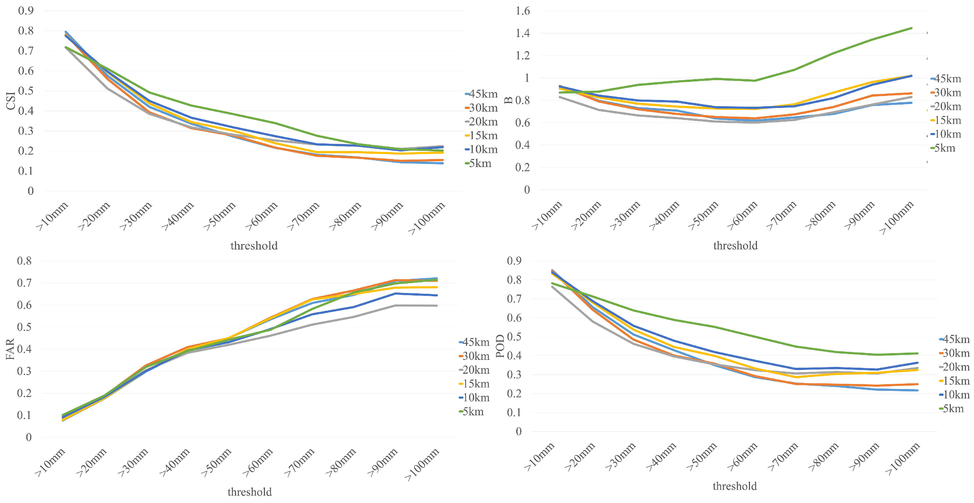
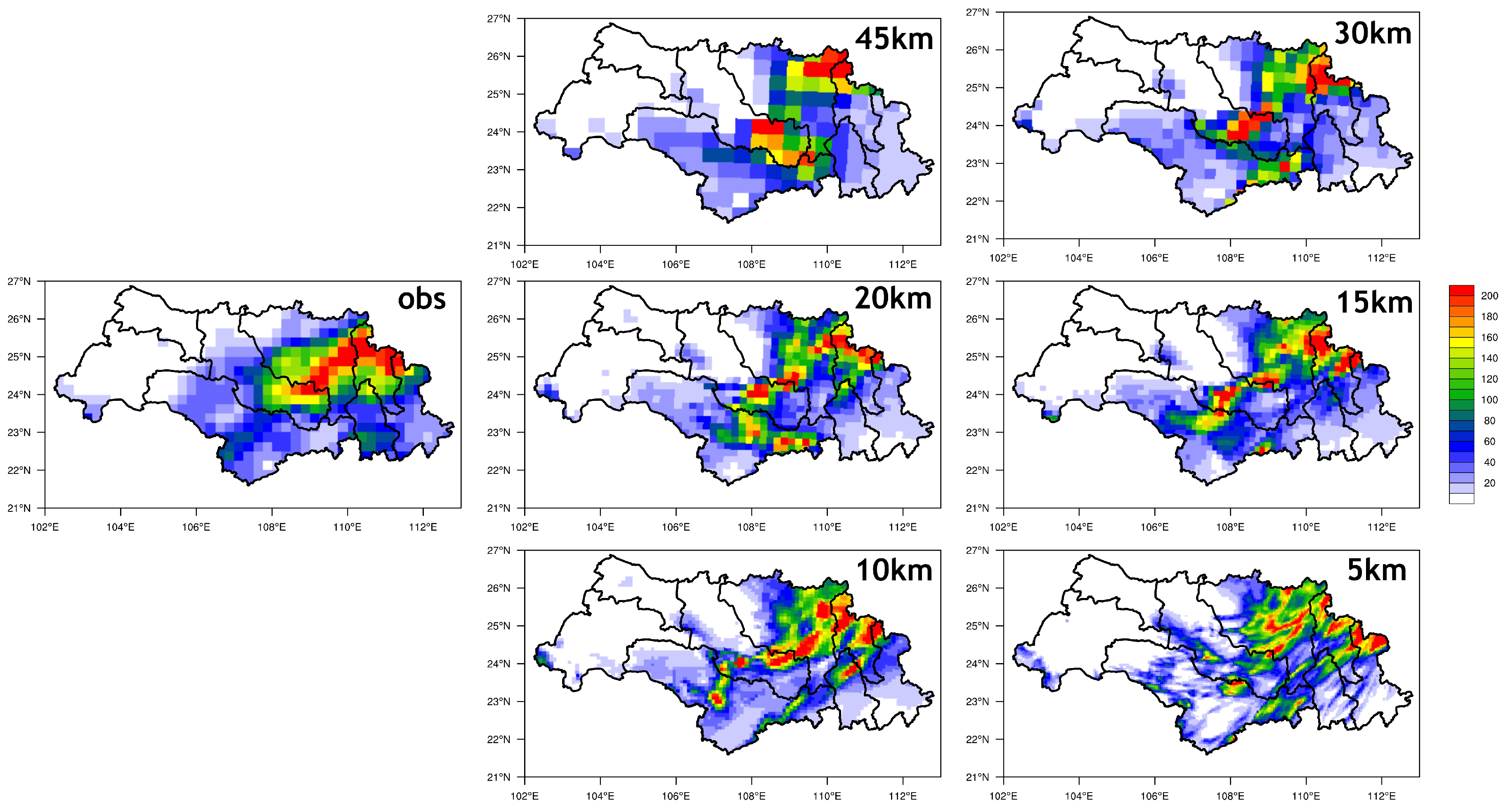
3.1. Influence of Horizontal Resolution and Domain Size on Simulations

The results from different horizontal resolutions indicated that the WRF model was able to simulate all precipitation processes from Case 1 to Case 7. In order to investigate the downscaling ability of the WRF model at different horizontal resolutions, the Bias (B), false alarm rate (FAR), and probability of detection (POD) indexes were calculated at different thresholds. From Figure 4, we can see that the CSI scores increased as the horizontal resolution got higher. Especially when the horizontal resolution was 5 km, the CSI score was always the highest compared to the other resolutions. The POD indexes showed results similar to the CSI scores. Although the CSI and POD scores at a horizontal resolution of 10 km were lower than that of 5 km, the results were better than other resolutions.
When the bias and FAR are taken into consideration, higher horizontal resolution always resulted in higher bias and FAR scores. When the threshold was greater than 60 mm/day, the bias increased significantly at a horizontal resolution of 5 km. The biases of 15 km and 10 km were almost the same, which were close to the value of 1 when the threshold was greater than 100 mm/day. Although the FAR scores at a horizontal resolution of 10 km were higher than that of 20 km, it was much lower than other resolutions.
Differences still exist, especially for the simulation of rainstorm centers. Here, we selected Case 5 as a typical case because the amount of areal average precipitation and maximum grid precipitation was greatest when compared with other cases. It was obvious that the main rain belt which covered southern GJ and the center of the HSH sub-basin was well captured by all horizontal resolutions (Figure 5). However, the location of rainstorm center showed great diversity with different resolutions. When the horizontal resolution was below 15 km, the rainstorm center located in the center of the QLJ sub-basin was not well captured. The amount of simulated precipitation was about 140 mm/day, while the observed precipitation exceeded 200 mm/day. Although the distribution at a horizontal resolution of 10 km and 5 km was much closer than observation, the discontinuity of rain bands at a horizontal resolution of 5 km made it more difficult to locate the real rainstorm center.

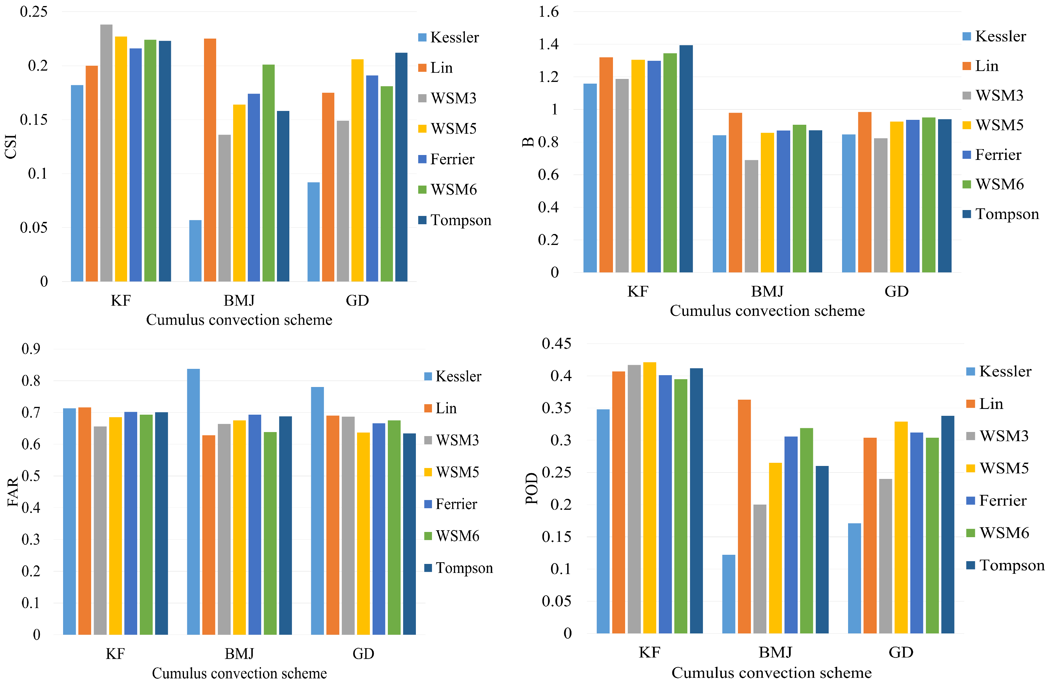
3.2. Influence of Physical Parameterization Scheme on Simulations

The domain configuration of physical parameterization sensitivity tests was based on the results of horizontal resolution sensitivity tests, and the outer domain was d01 with a horizontal resolution of 30 km and the inner domain was d02 with a horizontal resolution of 10 km. The B, FAR, and POD scores at a threshold of 100 mm/day were calculated for physical parameterization sensitivity tests as well (Figure 6). Greater differences were observed when different cumulus convective schemes and microphysics schemes were used. Although the KF convective scheme always leads to higher CSI scores when compared with the other two convective schemes, its biases were always higher than others. When the cumulus convective scheme was the BMJ scheme, the CSI score was greatly influenced by the choice of microphysics scheme. It was clear that the combination of BMJ convective scheme and Lin microphysics scheme always leads to higher CSI and POD scores, and lower biases and FAR scores than other combinations.

3.3. Evaluation of Precipitation Forecast with the Optimized Configuration

Based on the results of horizontal resolution and domain size sensitivity tests, we concluded that the optimized configuration of the WRF model for the Xijiang Basin was the two domain nested strategy, in which the outer domain was d01 with a horizontal resolution of 30 km while the inner domain was d02 with a horizontal resolution of 10 km. Meanwhile, the Lin microphysics parameterization scheme and the BMJ cumulus convective parameterization scheme was the best configuration for physical parameterizations. In order to evaluate the performance of the optimized configuration, the WRF model was integrated for 96 h and initialized daily from 1st June to 31st August in 2013 and 2014, driven by GFS 1 degree forecast data and updated lateral boundary condition every 6 h.

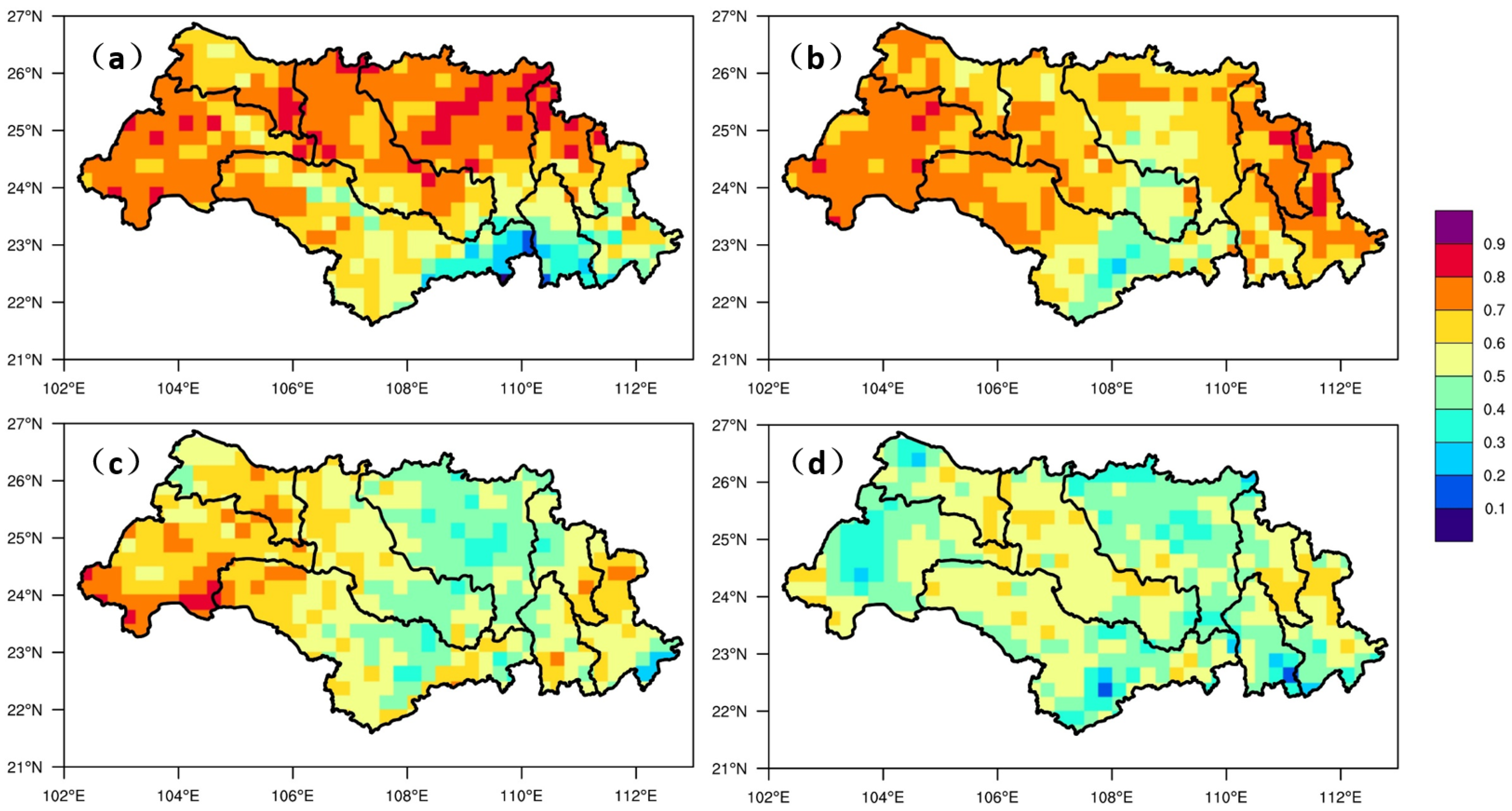
3.3.1. Evaluation of Grid Point Forecast

From the result of the correlation coefficient of 24 h total grid point precipitation between prediction and observation, it was clear that the WRF model with optimized configuration performed well (Figure 7).
The R values of GJ and QLJ sub-basins were >0.7 at a lead time of 24 h. However, the results showed significant regional variations, and the differences between north and south regions were up to 0.4 when the lead time was 24 h. The R values for YJ and XUN sub-basins were <0.3. The differences reduced with the extension of the forecast period, because the forecast accuracy in the north region decreased, while the forecast accuracy in the south region remained the same.
The spatial distribution of CSI and bias scores at a threshold of 0.1 mm/day are shown in Figure 8 and Figure 9. The CSI score for the whole Xijiang Basin was >0.4 for all forecast periods, confirming the accuracy of the optimized configuration. However, the highest CSI score was located in the eastern Xijiang River Basin, which differs with the results of R. Bias was >1.0 for almost all locations and forecast periods, meaning that the forecast precipitation area was greater than that of the observed data. BPJ and the northern YJ sub-basins showed the greatest biases when compared with other sub-basins, and the bias scores reached a value of 1.5.
In order to have a more reasonable evaluation of precipitation forecasts over Xijiang Basin, the percentiles of the climatological distribution of observed 24 h precipitation was taken into consideration. However, it was difficult to determine a fixed rainfall amount for all the gridpoints, due to the lack of observations for such a long period. We finally decided to utilize a threshold of 20 mm/day as the 90th percentile daily precipitation based on the results from Wu et al. [34]. The CSI and Bias scores at a threshold of 20 mm/day were shown in Figure 10 and Figure 11.
It was obvious that the CSI score at a threshold of 20 mm/day was much lower than that of 0.1 mm/day. When the lead time was 24 h, the CSI score reached a value of above 0.5 in NPJ, HSH, QLJ and GJ sub-basins. However, the forecast skill decreased significantly as the extension of forecast periods, especially in the QLJ sub-basin. Large biases were observed in NPJ, YJ, XUN, and XIJ sub-basins, where the bias scores were greater than 1.9. Meanwhile, the HSH sub-basin showed slight biases for all forecast periods.

3.3.2. Evaluation of Average Precipitation Forecast

The observed mean precipitation of each sub-basin was calculated and divided into three classes of rainfall amount: 0–10 mm/day, 10–20 mm/day, and >20 mm/day, based on the analysis of percentiles in previous sections.
For the MRE results (Figure 12), the WRF model showed remarkable differences among different sub-basins. When the observed average precipitation was lower than 10 mm/day, the MRE values of most sub-basins were higher than 100%, which indicated that a wet bias existed for most sub-basins. The MRE value decreased as the observed mean precipitation increased. The MRE values were between −50% and 150% for all sub-basins when the observed precipitation was between 10 and 20 mm/day, and the value of HSH sub-basin was lowest when compared with other sub-basins. A dry bias was observed for most sub-basins when the area average precipitation was beyond 20 mm/day. However, the values of mean relative error, which were between −70% and 50% for most sub-basins, were relatively low when compared with the other two classes of rainfall amount.

3.4. Discussion

Higher horizontal resolution may provide a more detailed description of rainbands, and always leads to higher precipitation intensity, and is capable of resolving mesoscale weather systems (the main factor in precipitation generation). A lot of studies have studied the causes of extreme precipitation for case 5, and pointed out the mesocale low altitude jet flow and the orographic lift effects contribute most to the generation of precipitation in the QLJ sub-basin [35,36]. Although the rainstorm centers located in the GJ and HSH sub-basins are well captured at any horizontal resolution, the rainstorm center over the QLJ sub-basin is missed unless the horizontal resolution is increased to 10 km. However, the improvement of forecast accuracy by increasing the horizontal resolution is limited; such a result is similar to those of Bresch et al. [37] and Gallus [38]. The appearance of discontinuous rainbands and the intensity of forecast precipitation far exceed the observation when the grid resolution is beyond 10 km, which indicates that high horizontal resolution may explicitly resolve mesoscale features. However, this may not be true because the spatial resolution of observed data does not allow a proper term of verification when the detailed forecast rainfall field at a grid spacing lower than 25 km. Further investigations are needed to improve the verification of precipitation forecasts at a resolution higher than 10 km.
The selection of physical parameterization schemes used by the model simulations is the most important factor, because microphysics and convective parameterization directly influence the generation of precipitation. The main differences of microphysics schemes are shown in Table 5. Among these seven microphysics schemes, the Lin, Ferrier, WSM6, and Thompson scheme take both the ice phase transformation and mixed-phase clouds transformation into consideration. However, the forecast skills of these schemes are not always higher than others, which indicates that microphysics schemes must coordinate with other parameterization schemes to give a better description of the microphysical processes. The Kain–Fritsch convective scheme is developed from the Fritsch–Chappell scheme, which considered both the downdrafts and convective available potential energy (CAPE). However, the deep convection processes—which are also of great importance to the Xijiang Basin—are not well described in the KF scheme. The BMJ scheme takes both the shallow and deep convection processes into consideration, and a modified moist-adiabatic profile is used as the convective adjustment reference profile. This may contribute to the higher forecast skill of the BMJ scheme when the Lin microphysics scheme is used. The GD ensemble scheme runs various cumulus trigger schemes for each grid, and the results are averaged to the model. Although this treatment takes the uncertainties of convective processes into account, the deep convection may play a more important role in the generation of precipitation over the Xijiang Basin.
The results of 2013–2014 simulations using the optimized configuration indicate that the optimized configuration of the WRF model is capable of forecasting precipitation over complex topography, and spatial distribution of the CSI scores are similar to the climatological distribution of flood season precipitation shown in Figure 13. Forecast accuracy varies among different sub-basins, and the WRF model always shows higher forecast accuracy in QLJ, HSH, and BPJ sub-basins, where the climatological precipitation is between 500 and 800 mm. Biases exist for the western NPJ sub-basin and the northern XIJ sub-basin, which indicate that the WRF model at a horizontal resolution of 10 km may have overestimated the convection processes in these areas. The precipitation forecast skill at the southern YJ sub-basin is always lowest when compared with other sub-basins, while the climatological precipitation is highest, with a value of above 1000 mm. A higher horizontal resolution of the WRF model may be needed for this area to resolve mesoscale convective system (MCS) at small scales.

4. Conclusions

In this study, the influence of horizontal resolution, domain size, and physical parameterization scheme on WRF simulation results was analyzed using precipitation forecasts for the Xijiang Basin, southern China. On the basis of the results, it was found that increasing the horizontal resolution always led to a better description of precipitation field. However, the forecast skills are not always increased as the resolution is increased. Given that the horizontal resolution of the initial and lateral boundary condition is 1 ° × 1 ° , the most appropriate domain configuration is the inner domain d02 with a horizontal resolution of 10 km, while the outer domain is d01 with a horizontal resolution of 30 km. In addition, microphysics parameterization schemes and convective parameterization schemes are the most important consideration for precipitation forecasting. The performance of the WRF model improves when the Lin microphysics and the BMJ convective parameterization schemes are used. The evaluation of precipitation forecasts from 1st June to 31st August in 2013 and 2014 have proved that the sensitivity tests are effective for building a proper dynamic downscaling configuration for the Xijiang Basin.
Fuzzy verification—which takes the uncertainties in the observations into account—is suitable for discontinuous fields like precipitation [39]. This method would be used in the future to improve the verification process of WRF over the selected study area. In addition, further studies to improve the forecasting accuracy of heavy rains are needed. It should be noted that the performance of the WRF model varies from different sub-basins due to the complexity of the mesoscale convective system (MCS) over this region. The horizontal resolution may need to be improved to give a more accurate description of MCS in the southern YJ sub-basin. Furthermore, increased attention should be paid to improving the physical parameterizations. In this study, only the influence of different schemes on precipitation simulation was considered. Issues such as downdraft, entrainment-related parameters, and the consumption time of Convective Available Potential Energy (CAPE) should be calibrated to make a more realistic representation of the MCS. However, the modification of these issues must be coordinated with the weather system, which requires a lot of work, and has not been taken into consideration in this paper. The investigation of these issues should be the focus of future studies.

Acknowledgments

The authors thank for the very valuable comments from reviewers and constructive suggestions from managing editor and assistant editor which greatly improved the quality of the paper. This work is supported by the Special Public Sector Research Program of the Ministry of Water Resources (Grants No. 201301040, 201401008, and 201301070), the Foundation for the Author of National Excellent Doctoral Dissertation of P.R. China (Grant No. 201161), the Qing Lan Project and Program for New Century Excellent Talents in University (Grant No. NCET-12-0842), the Natural Science Foundation of Jiangsu Province of China (Grant No. BK20131368), and the National Science and Technology Major Projects (Grant No. 2012ZX07101-010).

Author Contributions

Guihua Lu and Zhiyong Wu conceived and designed the sensitivity tests. Yuan Li performed the computations and wrote the paper. Hai He analyzed the sensitivity data and gave valuable suggestions. Jun Shi participated in the discussion of the study. Yuexiong Ma and Shichuang Weng provided information about the research area. All the authors have read and approved the final manuscript.

Conflicts of Interest

The authors declare no conflict of interest.

References

  1. Wu, Z.Y.; Lin, Q.X.; Lu, G.H.; Wen, L.; Zhang, S.L.; Hu, J.W. A comprehensive assessment of extending the lead time of precipitation and streamflow forecast by using coupled hydrological and atmospheric modeling system. Disaster Adv. 2013, 6, 519–528. [Google Scholar]
  2. Wu, J.; Lu, G.H.; Wu, Z.Y. Flood forecasts based on multi-model ensemble precipitation forecasting using a coupled atmospheric-hydrological modeling system. Nat. Hazards 2014, 74, 325–340. [Google Scholar] [CrossRef]
  3. Baldauf, M.; Seifert, A.; Forstner, J.; Majewski, D.; Raschendorfer, M.; Reinhardt, T. Operational Convective-Scale Numerical Weather Prediction with the COSMO Model: Description and Sensitivities. Mon. Weather Rev. 2011, 139, 3887–3905. [Google Scholar] [CrossRef]
  4. Lee, C.S.; Ho, H.Y.; Lee, K.T.; Wang, Y.C.; Guo, W.D.; Chen, D.Y.C.; Hsiao, L.F.; Chen, C.H.; Chiang, C.C.; Yang, M.J.; et al. Assessment of sewer flooding model based on ensemble quantitative precipitation forecast. J. Hydrol. 2013, 506, 101–113. [Google Scholar] [CrossRef]
  5. Novak, D.R.; Bailey, C.; Brill, K.F.; Burke, P.; Hogsett, W.A.; Rausch, R.; Schichtel, M. Precipitation and Temperature Forecast Performance at the Weather Prediction Center. Weather Forecast. 2014, 29, 489–504. [Google Scholar] [CrossRef]
  6. Liu, X.L.; Coulibaly, P. Downscaling Ensemble Weather Predictions for Improved Week-2 Hydrologic Forecasting. J. Hydrometeoro. 2011, 12, 1564–1580. [Google Scholar] [CrossRef]
  7. Liu, J.; Bray, M.; Han, D.W. Sensitivity of the Weather Research and Forecasting (WRF) model to downscaling ratios and storm types in rainfall simulation. Hydrol. Process. 2012, 26, 3012–3031. [Google Scholar] [CrossRef]
  8. Matsangouras, I.; Pytharoulis, I.; Nastos, P. Numerical modeling and analysis of the effect of Greek complex topography on tornado genesis. Nat. Hazards Earth Syst. Sci. Discuss. 2014, 2, 1433–1464. [Google Scholar] [CrossRef]
  9. Teixeira, J.; Carvalho, A.; Luna, T.; Rocha, A. Sensitivity of the WRF model to the lower boundary in an extreme precipitation event-Madeira Island case study. Nat. Hazards Earth Syst. Sci. Discuss. 2013, 1, 5603–5641. [Google Scholar] [CrossRef]
  10. Carvalho, D.; Rocha, A.; Gomez-Gesteira, M.; Santos, C. A sensitivity study of the WRF model in wind simulation for an area of high wind energy. Environ. Model. Softw. 2012, 33, 23–34. [Google Scholar] [CrossRef]
  11. Zhang, H.L.; Pu, Z.X.; Zhang, X.B. Examination of Errors in Near-Surface Temperature and Wind from WRF Numerical Simulations in Regions of Complex Terrain. Weather Forecast. 2013, 28, 893–914. [Google Scholar] [CrossRef]
  12. Cheng, W.Y.Y.; Steenburgh, W.J. Evaluation of surface sensible weather forecasts by the WRF and the Eta Models over the western United States. Weather Forecast. 2005, 20, 812–821. [Google Scholar] [CrossRef]
  13. Wen, M.; Yang, S.; Vintzileos, A.; Higgins, W.; Zhang, R.H. Impacts of Model Resolutions and Initial Conditions on Predictions of the Asian Summer Monsoon by the NCEP Climate Forecast System. Weather Forecast. 2012, 27, 629–646. [Google Scholar] [CrossRef]
  14. Xue, Y.K.; Janjic, Z.; Dudhia, J.; Vasic, R.; de Sales, F. A review on regional dynamical downscaling in intraseasonal to seasonal simulation/prediction and major factors that affect downscaling ability. Atmos. Res. 2014, 147, 68–85. [Google Scholar] [CrossRef]
  15. Bhaskaran, B.; Ramachandran, A.; Jones, R.; Moufouma-Okia, W. Regional climate model applications on sub-regional scales over the Indian monsoon region: The role of domain size on downscaling uncertainty. J. Geophys. Res. Atmos. 2012, 117. [Google Scholar] [CrossRef]
  16. Haghroosta, T.; Ismail, W.; Ghafarian, P.; Barekati, S. The efficiency of the WRF model for simulating typhoons. Nat. Hazards Earth Syst. Sci. Discuss. 2014, 2, 287–313. [Google Scholar] [CrossRef]
  17. Lowrey, M.R.K.; Yang, Z.L. Assessing the Capability of a Regional-Scale Weather Model to Simulate Extreme Precipitation Patterns and Flooding in Central Texas. Weather Forecast. 2008, 23, 1102–1126. [Google Scholar] [CrossRef]
  18. Zhang, S.R.; Lu, X.X.; Higgitt, D.L.; Chen, C.T.A.; Han, J.T.; Sun, H.G. Recent changes of water discharge and sediment load in the Zhujiang (Pearl River) Basin, China. Glob. Planet. Change 2008, 60, 365–380. [Google Scholar] [CrossRef]
  19. Skamarock, W.; Klemp, J.; Dudhia, J.; Gill, D.; Barker, D.; Duda, M.; Huang, X.; Wang, W. A description of the Advanced Research WRF version 3. Available online: http://opensky.ucar.edu/islandora/object/ technotes:500 (accessed on 10 November 2016).
  20. Shen, Y.; Xiong, A.Y.; Wang, Y.; Xie, P.P. Performance of high-resolution satellite precipitation products over China. J. Geophys. Res. Atmos. 2010, 115. [Google Scholar] [CrossRef]
  21. Hong, S.Y.; Noh, Y.; Dudhia, J. A new vertical diffusion package with an explicit treatment of entrainment processes. Mon. Weather Rev. 2006, 134, 2318–2341. [Google Scholar] [CrossRef]
  22. Skamarock, W.; Klemp, J.; Dudhia, J.; Gill, D.; Barker, D.; Wang, W.; Powers, J.G. A description of the advanced research WRF version 2. Available online: http://oai.dtic.mil/oai/ oai?verb=getRecord&metadataPrefix=html&identifier=ADA487419 (accessed on 10 November 2016).
  23. Dudhia, J. Numerical Study of Convection Observed during the Winter Monsoon Experiment Using a Mesoscale Two-Dimensional Model. J. Atmos. Sci. 1989, 46, 3077–3107. [Google Scholar] [CrossRef]
  24. Mlawer, E.J.; Taubman, S.J.; Brown, P.D.; Iacono, M.J.; Clough, S.A. Radiative transfer for inhomogeneous atmospheres: RRTM, a validated correlated-k model for the longwave. J. Geophys. Res. Atmos. 1997, 102, 16663–16682. [Google Scholar] [CrossRef]
  25. Chen, F.; Dudhia, J. Coupling an advanced land surface-hydrology model with the Penn State-NCAR MM5 modeling system. Part I: Model implementation and sensitivity. Mon. Weather Rev. 2001, 129, 569–585. [Google Scholar] [CrossRef]
  26. Lin, Y.L.; Farley, R.D.; Orville, H.D. Bulk parameterization of the snow field in a cloud model. J. Clim. Appl. Meteorol. 1983, 22, 1065–1092. [Google Scholar] [CrossRef]
  27. Janjic, Z.I. The step-mountain eta coordinate model: Further developments of the convection, viscous sublayer, and turbulence closure schemes. Mon. Weather Rev. 1994, 122, 927–945. [Google Scholar] [CrossRef]
  28. Kessler, E. On the continuity and distribution of water substance in atmospheric circulations. Atmos. Res. 1996, 41, 179. [Google Scholar] [CrossRef]
  29. Hong, S.Y.; Lim, J.O.J. The WRF single-moment 6-class microphysics scheme (WSM6). Asia Pac. J. Atmos. Sci. 2006, 42, 129–151. [Google Scholar]
  30. Ferrier, B.S.; Houze, R.A., Jr. One-dimensional time-dependent modeling of GATE cumulonimbus convection. J. Atmos. Sci. 1989, 46, 330–352. [Google Scholar] [CrossRef]
  31. Thompson, G.; Field, P.R.; Rasmussen, R.M.; Hall, W.D. Explicit Forecasts of Winter Precipitation Using an Improved Bulk Microphysics Scheme. Part II: Implementation of a New Snow Parameterization. Mon. Weather Rev. 2008, 136, 5095–5115. [Google Scholar] [CrossRef]
  32. Kain, J.S. The Kain-Fritsch convective parameterization: An update. J. Appl. Meteorol. 2004, 43, 170–181. [Google Scholar] [CrossRef]
  33. Grell, G.A.; Devenyi, D. A generalized approach to parameterizing convection combining ensemble and data assimilation techniques. Geophys. Res. Lett. 2002, 29, 381–384. [Google Scholar] [CrossRef]
  34. Wu, L.; Liu, B.; Chen, X.; Lu, W. Uncertainty of Extreme Precipitation Threshold in Pearl River Basin. J. China Hydrol. 2013, 33, 59–64. [Google Scholar]
  35. Zhao, J.; Luo, J.; Gao, A.; Zeng, X. Analysis on a Heavy Rain Process in a Warm Sector in Guangxi in June 2008. Trop. Geogr. 2010, 30, 145–150. [Google Scholar]
  36. Chen, Y.; Nong, M. Diagnosis and numerical simulation of the persistent heavy rainfall in Guangxi in June 2008. J. Meteorol. Sci. 2010, 30, 250–255. [Google Scholar]
  37. Bresch, J.F.; Reed, R.J.; Albright, M.D. A polar-low development over the Bering Sea: Analysis, numerical simulation, and sensitivity experiments. Mon. Weather Rev. 1997, 125, 3109–3130. [Google Scholar] [CrossRef]
  38. Gallus, W.A. Eta simulations of three extreme precipitation events: Sensitivity to resolution and convective parameterization. Weather Forecast. 1999, 14, 405–426. [Google Scholar] [CrossRef]
  39. Ebert, E.E. Fuzzy verification of high-resolution gridded forecasts: A review and proposed framework. Meteorol. Appl. 2008, 15, 51–64. [Google Scholar] [CrossRef]
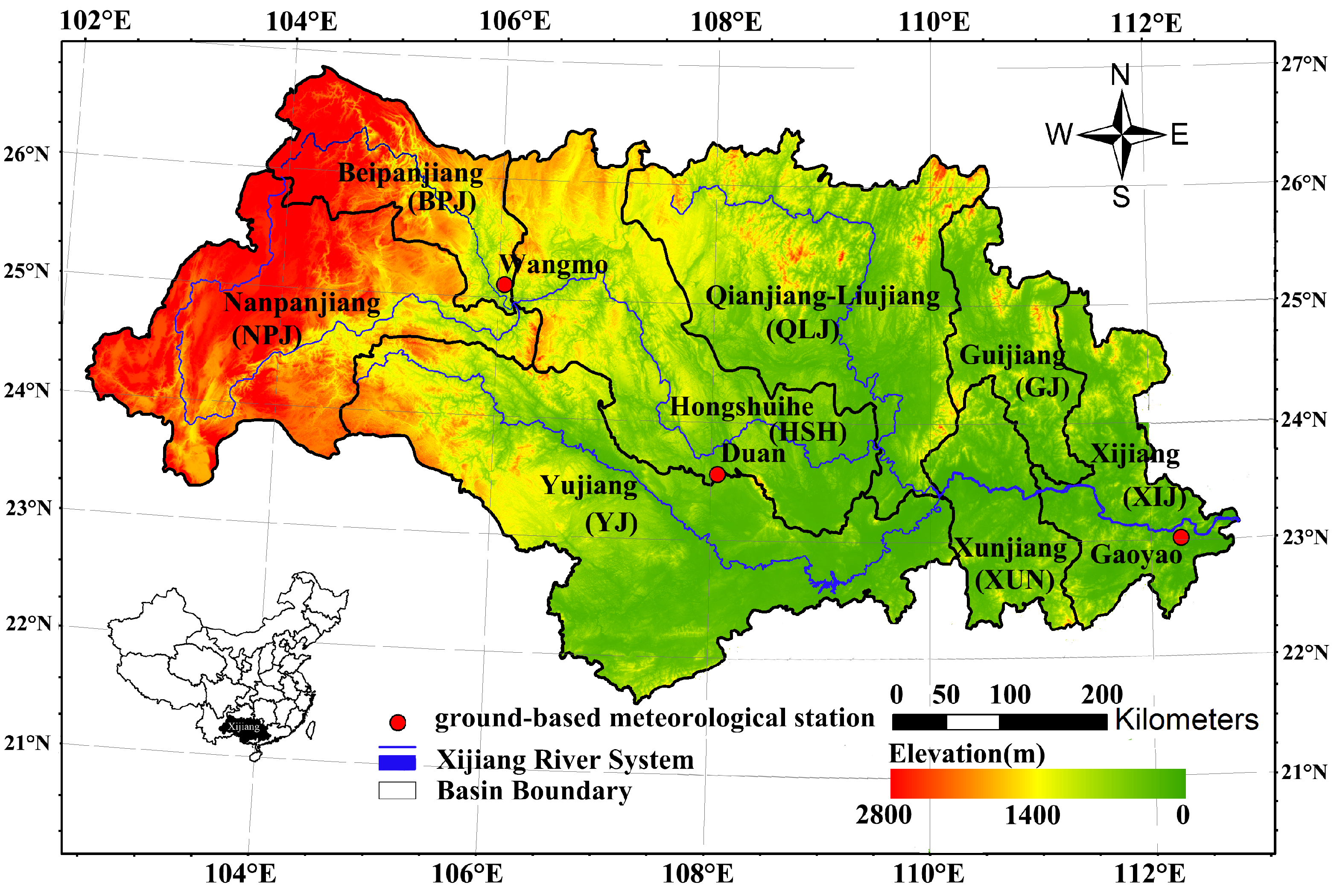
Figure 1. Regional map showing the location of three ground-based meteorological stations (red dots), the Xijiang River System (blue), and the local topography (elevation in metre) of the Xijiang Basin. The geographical location of the study region within China is shown in the small inset map (bottom left).
Atmosphere 07 00145 g001
Figure 2. Mean annual precipitation (mm/year) for the 1980–2010 period from the National Oceanic and Atmospheric Administration’s Climate Prediction Center (CPC) unified gauge-based analysis.
Atmosphere 07 00145 g002
Figure 3. Map of domain sizes of the d01–d03 simulations.
Atmosphere 07 00145 g003
Figure 4. Mean critical success index (CSI), bias (B) false alarm rate (FAR), and probability of detection (POD) scores for seven case studies at different horizontal resolutions (5 km, 10 km, 15 km, 20 km, 30 km, 45 km).
Atmosphere 07 00145 g004
Figure 5. Study region maps showing the observed and simulated precipitation (mm) distribution at different horizontal resolutions for Case 5.
Atmosphere 07 00145 g005
Figure 6. Mean CSI, B, FAR, and POD scores for seven case studies at different physical parameterization schemes (threshold ≥ 100 mm/day). (KF: Kain–Fritsch; BMJ: Betts–Miller–Janjic; GD: Grell–Devenyi; WSM: WRF–Single–Moment.)
Atmosphere 07 00145 g006
Figure 7. Study region maps showing the spatial distribution of correlation coefficient (R) in the Xijiang Basin. (a) 24 h lead time; (b) 48 h lead time; (c) 72 h lead time; (d) 96 h lead time.
Atmosphere 07 00145 g007
Figure 8. Study region maps showing the spatial distribution of CSI score (≥0.1 mm/day) in the Xijiang Basin. (a) 24 h lead time; (b) 48 h lead time; (c) 72 h lead time; (d) 96 h lead time.
Atmosphere 07 00145 g008
Figure 9. Study region maps showing the spatial distribution of Bias (≥0.1 mm/day) in the Xijiang Basin. (a) 24 h lead time; (b) 48 h lead time; (c) 72 h lead time; (d) 96 h lead time.
Atmosphere 07 00145 g009
Figure 10. Study region maps showing the spatial distribution of CSI score (≥20 mm/day) in the Xijiang Basin. (a) 24 h lead time; (b) 48 h lead time; (c) 72 h lead time; (d) 96 h lead time.
Atmosphere 07 00145 g010
Figure 11. Study region maps showing the spatial distribution of Bias (≥20 mm/day) in the Xijiang Basin. (a) 24 h lead time; (b) 48 h lead time; (c) 72 h lead time; (d) 96 h lead time.
Atmosphere 07 00145 g011
Figure 12. Mean relative error (MRE) of areal average forecast (yellow bars = 0–24 h; blue bars = 24–48 h; green bars = 48–72 h; red bars = 72–96 h) precipitation ((a) 0–10 mm; (b) 10–20 mm; (c) > 20 mm) for each sub-basin (BPJ = Beipanjiang; NPJ = Nanpanjiang; QLJ = Qianjiang–Liujiang; YJ = Yujiang; GJ = Guijiang; XUN = Xunjiang; XIJ = Xijiang).
Atmosphere 07 00145 g012
Figure 13. Mean precipitation from 1st June to 31st August for the 1980–2010 period.
Atmosphere 07 00145 g013
Table 1. The area of each sub-basin over Xijiang Basin.
Sub Basin Area ( km 2 )
Nanpanjiang (NPJ)67,191
Beipanjiang (BPJ)31,399
Hongshuihe (HSH)64,288
Yujiang (YJ)92,515
Qianjiang–Liujiang (QLJ)75,208
Guijiang (GJ)22,611
Xunjiang (XUN)21,694
Xijiang (XIJ)31,794
Table 2. Selected rainstorms over the Xijiang Basin.
EventOccurrence TimeAreal Average in
Proceedings of the
Precipitation (mm/day)
Weather SystemLocation of
Rainstorm Center
Maximum Grid
Precipitation
(mm/day)
Case10000 UTC
5–6 June 2005
54.1South Asia High and
Southwest monsoon
106.42 ° E 23.13 ° N 147 . 0
Case2 45.3Southwest vortex110.68 ° E 23.65 ° N 202 . 0
0000 UTCHigh-Level trough
21–22 June 2005and Shear line
Case30000 UTC57.4Tropical storm110.18 ° E 24.14 ° N 208.8
16–17 July 2006
Case4 47.0High and low109.4 ° E 24.35 ° N 228.0
0000 UTClevel jet
12–13 June 2007Shear Line
Case50000 UTC83.1South Asia High109.26 ° E 24.15 ° N 288 . 1
12–13 June 2008and Trough
Case6 49.9High-Level trough109.2 ° E 23.5 ° N 219 . 2
0000 UTCShear line and
3-4 July 2009Southwest monsoon
Case70000 UTC39.0Southwest vortex110.82 ° E 22.86 ° N 252 . 5
1–2 June 2010
Table 3. Nesting strategy and horizontal resolution for each domain.
Nesting StrategyHorizontal Resolution for Each Domain
Single domaind01 (45 km)
Single domaind01 (30 km)
Single domaind01 (20 km)
Two domain nestedd01 (45 km), d02 (15 km)
Two domain nestedd01 (30 km), d02 (10 km)
Three domain nestedd01 (45 km), d02 (15 km), d03 (5 km)
Table 4. Contingency table.
ForecastObservation
YESNO
YESab
NOcd
Table 5. Differences in microphysics schemes.
Microphysics SchemeIce Phase TransformationPhase Transformation of Mixed Phase Clouds
KesslerNONO
LinYESYES
WSM3YESNO
WSM5YESNO
FerrierYESYES
WSM6YESYES
ThompsonYESYES

