Article

Source Localization in the Duct Environment with the Adjoint of the PE Propagation Model

College of Meteorology and Oceanography, PLA University of Science and Technology, Nanjing 211101, China
Atmosphere 2015, 6(9), 1388-1398; https://doi.org/10.3390/atmos6091388
Submission received: 24 July 2015 / Revised: 8 September 2015 / Accepted: 10 September 2015 / Published: 22 September 2015

Abstract

:
Owing to the absorbing, refracting and scattering effects of the propagation medium, electromagnetic (EM) energy will degrade with the increment of propagation range, and the maximum value exists at the point of the radiating source. Employing this phenomenon, this paper introduces a novel approach to detect the location of EM transmitters in an atmospheric duct environment. Different from previous matched-field processing (MFP) methods, the proposed method determines the source location through reconstructing the forward propagation field pattern by the backward adjoint integration of the parabolic equation (PE) propagation model. With this method, the repeated computations of PE used in the MFP methods are not needed. The performance of the method is evaluated via numerical simulations, where the influences of the measurement noise and the geometry of the receiver array on the localization results are considered.

1. Introduction

In tropospheric electromagnetic (EM) wave propagations, the issues of determining source locations from range and/or range-difference observations gathered with an array of receivers have been studied a lot due to many important applications, such as surveillance, radio communications, and navigation [1,2,3].
Source localization is an inverse problem, and the solution is usually ill-posed, especially for multipath propagations caused by atmospheric duct environments. Previous studies treated these problems as an optimization problem and solved them by matching the observed signals with the predicted fields through the construction of an appropriate cost function [4,5,6]. Using these matching methods, repeated computations of a forward propagation model cannot be helped. In order to reduce computation time, some heuristic optimization methods are used, such as simulated annealing or a genetic algorithm.Even so, the amount of the iterations is still considerable, and the cost function may fall into a local minimum.
Owing to the absorbing, refracting and scattering effect of the propagation medium, EM energy will degrade with the increment of the propagation range, and the maximum value exists at the point of the radiating source. Employing this phenomenon, the maximum energy point, i.e., the source location can be determined by reconstructing the spatial propagation fields. Given known environmental parameters, this paper proposes a method for source localization using backward propagation of the adjoint integration of the parabolic equation (PE) model. With this method, repeated computations of the forward propagation model are not needed.
The paper will be organized in the following manner: The PE propagation approach is described in Section 2. Section 3 gives the basic concepts of the adjoint operator and its application to the considered localization problem. The numerical experiments for propagation field reconstruction and source localization are given in Section 4, where detailed discussions about the measurement noise and the receiver array geometry that affect the localization results are presented. In Section 5, the basic conclusions are summarized.

2. Propagation Model

In the past decades, the PE approach has been the most popular method to model EM wave propagation in the troposphere [7,8,9,10,11,12]. The PE method has advantages of giving an exact full-wave field solution for range-dependent environments. Under certain assumptions of the scalar Helmholtz wave equation, the PE can be derived as [7],
2 u ( x , z ) z 2 + 2 i k 0 u ( x , z ) x + k 0 2 [ m 2 ( x , z ) 1 ] u ( x , z ) = 0
where u is a complex scalar component, for vertical polarization, it represents the magnetic field, and for horizontal polarization, it represents the electric field. x and z represent the range the height, respectively. k 0 is the free-space wave number. m is the modified refractive index and is defined by m = n + z/ae, where n is the refractive index and ae is the radius of the Earth. Owing to the fact that m approximates to unity, modified refractivity M, defined by M = 106 × (m − 1), is adopted for the environmental input.
Equation (1), in conjunction with the proper boundary conditions (in the following numerical computations, a smooth perfectly conducting surface is used to simulate the lower boundary, and a cosine-tapered window is applied to the upper one-fourth of the field to hold back nonphysical upper boundary reflections), is an initial value problem that can be solved by the Fourier split-step numerical method as:
u ( x k + 1 , z ) = exp ( i k 0 2 ( m 2 1 ) δ x ) F 1 { exp ( i p 2 δ x 2 k 0 ) F { u ( x k , z ) } }
where F[·] is the Fourier transform, F−1[·] is the inverse Fourier transform, and p is the transform variable. δx = xk+1−xk is the range increment. For detailed Fourier split-step PE solution, the readers can refer to [8]. Using Equation (2) to simulate propagations, the initial field u0 at the range x0 = 0 should be given, which is determined by the source system parameters.

3. Adjoint Operator

For inverse problems, a physical model can be looked as an abstract system H which maps a vector of X onto a vector of Y, where X represents control variables and Y represents the needed predictions corresponding to observations [13,14,15,16,17,18]. The goal is to derive information about X (unknown) from Y (known). The tangent linear model (TLM) maps δ X onto δ Y , where δ X represents variations of the control variables and δ Y represents variations of the model prediction. The TLM is defined by linearizing the model around a given point X 0 and it is actually the Jacobian matri A ( X 0 ) of the mapping H. The adjoint A * ( X 0 ) of the Jacobian represents adjoint model that maps in the reverse direction and calculates the effects of the control variables on abnormal model predictions. The relationship between the tangent and the adjoint operator is:
( A v , w ) = ( v , A * w )
where (,) is an appropriate inner product. If the Jacobian matrix A is real, A* is the transpose matrix of A; while A is complex, A* is the conjugate transpose matrix of A.
The adjoint of the PE propagation model has been widely used in atmospheric refractivity estimations [19,20,21] and ocean acoustic inversions [22,23,24], where the source information is assumed to be known and the environmental physical characteristics are estimated by matching the observed signals with predicted fields with a gradient-based minimization algorithm. For the source localization problem considered in this paper, the environmental conditions are assumed to be known. Then, the uncertainty of the observed signals is only determined by the source initial fields. To fix observation geometry, different source locations correspond to different initial fields.
From Equation (2), it is clear that the fields at range xk+1 have a linear relationship to the fields at range xk, and in turn, to the fields at range x0. That is, if the control variables are selected to the initial fields u0, the form of the tangent linear model is equivalent to the original propagation model. Using the definition of the adjoint operator A*, it is obtained:
( A ( u k ) u k , u k + 1 ) = ( u k , A * ( u k ) u k + 1 )
where uk+1 in the right hand side can be regarded as a driving of the adjoint model. From equation (4), given the measurement fields at the range xk+1, the fields at previous ranges can be reconstructed by the backward propagation of the adjoint integration (using the Fourier split-step method to solve PE, the discrete Fourier transform, by way of the fast Fourier transform, i.e., FFT, is actually used). Owing to FFT is a unitary operator, its adjoint equals its inverse [25]. Employing this property, the adjoint of the PE model can be easily solved by the backward Fourier split-step method. As illustrated above, the source location can be easily determined by finding the maximum field strength point from the reconstructed field strength pattern.

4. Numerical Experiments and Analysis

The approach described above is novel in that it introduces the backward propagation of the adjoint integration for the source localization problem. With this method, an appropriate cost function by matching the observed signals with the predicted fields is not needed, and the repeated computations of the forward propagation model are avoided. Owing to the real data are not available, numerical experiments are performed to test the theoretical method.
In the following numerical computations, the refractive conditions are assumed to be horizontally homogeneous with a 50-m surface-based duct. A horizontal polarized Gaussain source located at a height of 30 m above the mean sea level is used to simulate the initial field at x0 = 0. The detailed refractivity parameters and the source system parameters are shown in Table 1 and Table 2, respectively. These parameters are used as the input for the PE model to construct the synthetic measurements received by a vertical array at the range 100 km. That is, to the mean sea level of the receiver array, the source location can be noted as (range, height) = (100 km, 30 m).
Table 1. Refractivity parameters.
Height (m)Refractivity (M-units)
0330
50320
1050438
Table 2. A horizontal polarized Gaussain source parameters.
Frequency (MHz)Beamwidth (°)Elevation (°)Height (m)
50000.4030

4.1. Propagation Fields Reconstruction

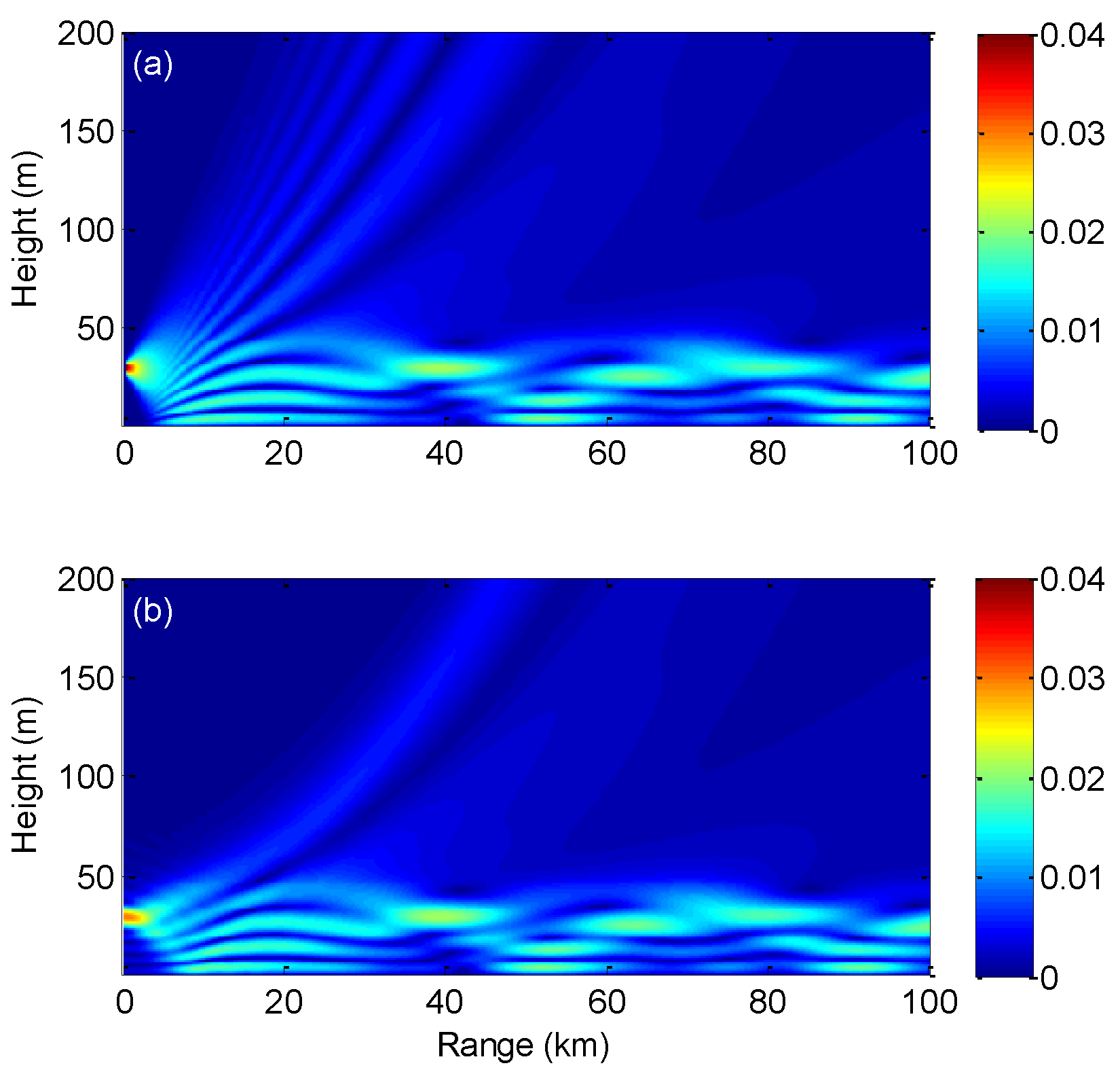
Figure 1a gives the coverage diagram of the field strength | u | , i.e., the absolute value of u , computed by the forward PE model(see Equation(2)). The computation domain is set to be: the maximum range 100 km, the range bin 200 m, the maximum height 1024 m, and the height bin 1 m (that is, the FFT transform size is 1024 = 210). It is seen that, owing to the duct propagation, most of the EM energy is captured in the duct layer. The focus center of the field strength is at the source location and the strength behaves, cyclical downswing, with the increment of the propagation range.
In the backward adjoint propagation modeling, the refractivity profile is assumed to be known. Set the synthetic field at the terminal range, 100 km, as the input to the adjoint model, the fields at previous ranges are computed in Figure 1b. Comparing Figure 1a with Figure 1b, the basic propagation characteristics of the forward fields are reconstructed by the adjoint fields, but the whole field strength is weakened slightly. This is because in the forward and adjoint modeling, the upper one-fourth of the field is filtered to prevent reflections from the nonphysical upper boundary. However, the maximum field strength point can still be easily found around the source location.
Figure 1. Coverage diagrams of the field strength. (a) Forward propagation modeling of the PE model, and (b) backward propagation modeling of the adjoint of the PE model.
Atmosphere 06 01388 g001
The propagation field reconstructions without an additive filtering window are shown in the appendix, where it can be seen that the forward propagation fields can be exactly reconstructed by the backward adjoint integration.
In practical operations, the available measurements are often contaminated by noise, and data with such high vertical resolutions are impossible. In the following, the influences of the noise and the receiver geometry to the localization results are considered.

4.2. Noise Influence

This section considers the influence of the measurement noise to the source localization results. Here, the vertical receiver array still contains 1024 elements with height interval of 1 m, but different random white noise is added to the received EM signals, as well as the impossible uncertainty of the refractivity measurement is also considered.
In case of the refractivity is exactly known, 
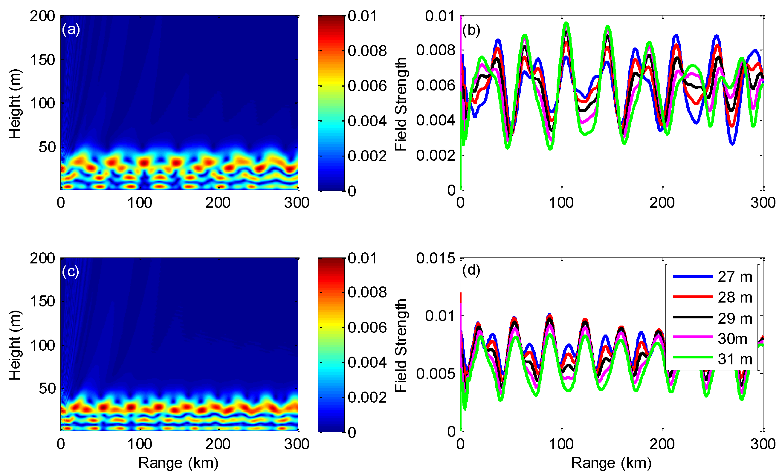
Figure 2a gives the backward propagation fields with 15% random white noise added to the EM measurements, where the range of the receiver array is noted as 0 m and the backward propagation range is extended to 300 km. From Figure 2a, it is clear that the maximum field strength appears around (100 km, 30 m). According to the above analysis, the position of the maximum strength corresponds to the source location. Additionally, it is seen that above the source location exists as a big “V” blind energy zone that is caused by the directional transmitting source and the size of ‘V’ is determined by the 3 dB beamwidth. Moreover, there exists a reverse ‘V’ blind energy zone below the source location. Although similar zones also exist at ranges of 65 km and 135 km, the shape at a range of 100 km is clearer. Near the vertical receiver array, the reconstructed field looks a little blurry, which is caused by the EM measurement noise. Figure 2b shows the field strength along the propagation range at different heights, which further validates the source localization results. Figure 2c,d gives the backward propagation fields with 30% additive random white noise. The source location can still be easily found from the coverage diagram, but the fields near the vertical receiver array look more blurry than in Figure 2a, owing to the more noisy EM measurements.
Figure 2. The influences of the EM measurement noise to the source localization results. (a) Coverage diagram of the backward propagation field with 15% random white noise added to the EM measurements, (b) the field strength along the propagation range at different heights of (a), (c) and (d) are, respectively, identical to (a) and (b), but with 30% additive random white noise.
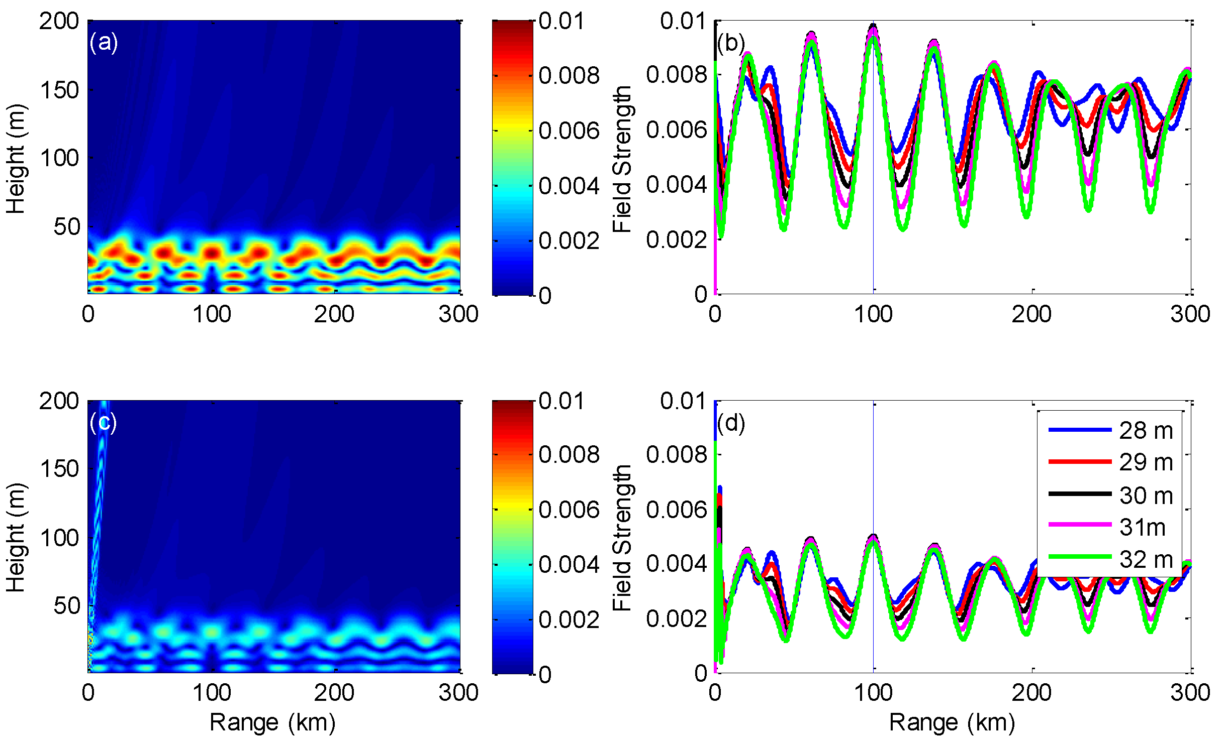
Atmosphere 06 01388 g002
Figure 3. 
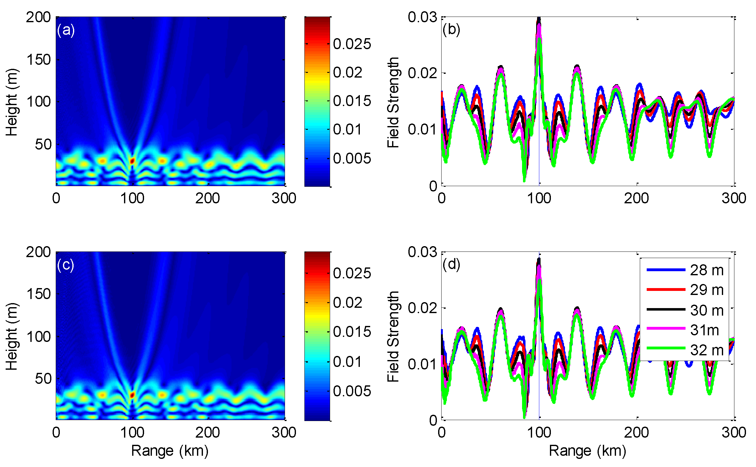
The influences of the refractivity measurement noise to the source localization results. (a) Coverage diagram of the backward propagation field with duct height of 55 m and duct strength of 10 M-units, (b) the field strength along the propagation range at different heights of (a), (c) and (d) are, respectively, identical to (a) and (b), but with duct height of 50 m and duct strength of 12 M-units.
Atmosphere 06 01388 g003
In practical operations, it is difficult to absolutely exactly ensure the refractivity measurements. Refractivity measurement noise will inevitably influence the source localization results. Maintaining 30% random white noise added to the EM measurements, Figure 3a shows the backward propagation fields with a 55-m duct height and 10 M-units of duct strength (i.e., 5 m higher than the true duct height).It is clear that, in the first 100 km propagation range, the field strengthlooks very blurry, and the big “V” and reverse “V” blind energy zones shift off 100 km range to some extent. With the aid of field strength along the propagation range in Figure 3b, the maximum energy point, i.e., source position can be determined at 105 km, 32 m.
Figure 3c gives the backward propagation fields with a 50-m duct height and 12 M-units of duct strength (i.e., 2 M-units stronger than the true duct strength). Compared with Figure 3a, the reverse ‘V’ blind energy zone nearly disappears in Figure 3c and the maximum energy point deviates over 10 km away from the true source position. Combining Figure 3c with Figure 3d, the estimated location is 87 km, 27 m. Although the change of duct height is larger than the duct strength (both increase by 10%, respectively), the localization result of duct height departure is better than that of duct strength departure. This may be due to the fact that, in the duct propagations, EM energy distribution depends more on duct strength than on duct height.

4.3. Receiver Geometry Influence

The influence of the receiver geometry to the source localization results is considered in this section. Two different geometries are used. In Case 1, the transmitted signal is received by a vertical array of 25 elements uniformly distributed between 2 m and 50 m. In Case 2, the same number receivers are uniformly distributed between 4 m and 100 m. In the following, Figure 4 gives the results without noise, and Figure 5 gives the results with both EM measurement noise and refractivity uncertainties.
Figure 4. 
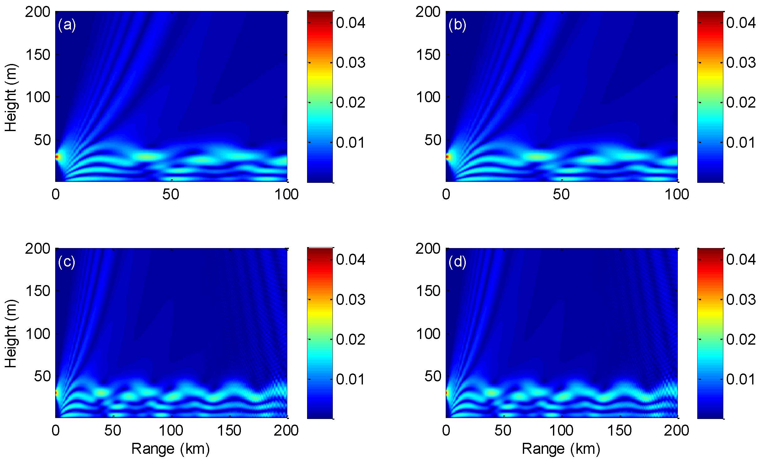
The influences of the receiver geometry to the source localization results. (a) Coverage diagram of the backward propagation field with Case 1 geometry, (b) the field strength along the propagation range at different heights of (a), (c), and (d) are, respectively, identical to (a) and (b), but with Case 2 geometry.
Atmosphere 06 01388 g004
Figure 4a gives the backward propagation fields with 2–50 m receiver geometry. Due to lacking of the enough received signals, the source location is not easily determined, as shown in Figure 2. From the energy-focused districts, it is certain that the source height is around 30 m, but there exist several local maximum energy points. To determine the source location exactly, the field strength along the propagation range shown in Figure 4b will be helpful. Combining Figure 4a with Figure 4b, the source location can be fixed at 100 km, 30 m, by selecting the middle one among the three local maximum values. The reverse “V” shape blind energy zone in Figure 4a can also give an assistance to validate the localization results.
Figure 4c,d gives the backward propagation fields with 4–100 m receiver geometry. The field strength with this geometry looks like only half that of Case 1. This is because the energy above the duct height (50 m) contributes slightly to the duct layer propagation. The singular highlight fields near the receiver array may be caused the sparse received signals. These abnormal fields should be ignored for the localization results. Combining Figure 4c with Figure 4d, the source location can also be exactly determined with the same analysis method.
Figure 5 shows the backward propagation fields with 2–50 m receiver geometry, combining 30% EM measurement noise with refractivity uncertainties (the same as the refractivity changes in Figure 3). Again, with refractivity noise, the estimated source position does not match very well with the true source point. With 10% duct height increment, see Figure 5a,b, the maximum energy point can be determined at 105 km, 31 m; while with 10% duct strength increment, see Figure 5c,d, the maximum energy point can be determined at 88.5 km, 27 m. Comparing Figure 4 and Figure 5 with Figure 2 and Figure 3, it is found that, although getting unabridged received signals is not necessary, the decrease of the receiver number increases the difficulty of finding the maximum energy point. If receiver numbers are dropped further, it will make the localization results more inconclusive.
Figure 5. The influences of the receiver geometry (Case 1) and measurement noise to the source localization results. (a) Coverage diagram of the backward propagation field with duct height of 55 m and duct strength of 10 M-units, (b) the field strength along the propagation range at different heights of (a), (c) and (d) are, respectively, identical to (a) and (b), but with a duct height of 50 m and duct strength of 12 M-units.
Atmosphere 06 01388 g005

5. Conclusions

A novel approach to localize the source position from reconstructing the forward propagation field strength by the backward adjoint integration of the PE model has been proposed. The source location can be easily determined by finding the maximum field strength point in the reconstructed field pattern, which avoids the massive computations of the forward propagation model. The results based on the above numerical experiments are summarized as follows: (1) with unabridged terminal received signals and exact refractivity measurements, the forward propagation fields can be exactly reconstructed by the backward adjoint integration and the source location can be easily found; (2) with the decrease of the received signals, several local maximum field strength points will emerge, and the strength profiles along the propagation range are helpful to eliminate the mendacious source locations; and (3) the EM measurement noise has little influence on the localization results, while the influence of refractivity uncertainties, especially the departure of the duct strength, cannot be ignored. However, within 10% variation of the duct parameters, the estimated results are acceptable.
Even though promising, these results are preliminary and need to be validated by real measurement data. The refractive conditions are assumed to be known or keep good confidence level in the proposed method. Unfortunately, as a result of limitations in atmospheric modeling and measurement capabilities, accurate prior knowledge of the environmental parameters is difficult. How to apply the adjoint method for joint environmental parameter estimation and source localization is also an interesting issue for future work.

Acknowledgments

This work was supported by the National Natural Science Foundation of China (41405025), and Jiangsu Province Natural Science Foundation of China (BK20140064).

Conflicts of Interest

The authors declare no conflict of interest.

Appendix: Propagation Fields Reconstruction without Filtering Window

Figure A1 shows the backward propagation field reconstruction without a filtering window added to the upper one-fourth of the field. Figure A1a,c is the forward propagation field computed by the PE model with the input parameters given in Table 1 and Table 2. Figure A1b,d is the reconstructed fields computed by the adjoint of the PE model. It is clear that, without a filtering window, the reconstructed field is exactly the same as the forward propagation one. Figure A1c,d extends the propagation range to 200 km, where it is seen that, beyond 150 km, the fields are contaminated by the reflections from the nonphysical upper boundary. This just shows an example of how well using the backward adjoint integration to reconstruct the forward propagations can be. To simulate the practical propagations, a filtering window should be used, which has only limited effects on the source localization results, seeing numerical experiments given in Section 4.
Figure A1. Coverage diagrams of the field strength without a cosine-tapered filtering window used. (a) Forward propagation modeling of the PE model, and (b) backward propagation modeling of the adjoint of the PE model, (c) and (d) are, respectively, identical to (a) and (b), but extending the propagation range to 200 km.
Atmosphere 06 01388 g006

References

  1. Cheung, K.W.; So, H.C. A multidimensional scaling framework for mobile location using time-of-arrival measurements. IEEE Trans. Signal Process. 2005, 53, 460–470. [Google Scholar]
  2. Sayed, A.H.; Tarighat, A.; Khajehnouri, N. Network-based wireless location: Challenges faced in developing techniques for accurate wireless location information. IEEE Signal Process. Mag. 2015, 22, 24–40. [Google Scholar] [CrossRef]
  3. Beck, A.; Stoica, P.; Li, J. Exact and approximate solutions of source localization problems. IEEE Trans. Signal Process. 2008, 56, 1770–1778. [Google Scholar] [CrossRef]
  4. Gingras, D.F.; Gerstoft, P.; Gerr, N.L. Electromagnetic matched field processing: Basic concepts and tropospheric simulations. IEEE Trans. Antennas Propag. 1997, 45, 1536–1545. [Google Scholar] [CrossRef]
  5. Spencer, T.A.; Walker, R.A.; Hawkes, R.M. Inverse diffraction parabolic wave equation localization system (IDPELS). J. Glob. Position. Syst. 2005, 4, 245–247. [Google Scholar] [CrossRef]
  6. Zhao, X. Evaporation duct height estimation and source localization from field measurements at an array of radio receivers. IEEE Trans. Antennas Propag. 2012, 60, 1020–1025. [Google Scholar] [CrossRef]
  7. Dockery, G.D. Modeling electromagnetic wave propagation in the troposphere using the parabolic equation. IEEE Trans. Antennas Propag. 1988, 36, 1464–1470. [Google Scholar] [CrossRef]
  8. Kuttler, J.R.; Dockery, G.D. Theoretical description of the parabolic approximation/Fourier split-step method of representing electromagnetic propagation in the troposphere. Radio Sci. 1991, 26, 381–393. [Google Scholar] [CrossRef]
  9. Craig, K.H.; Levy, M.F. Parabolic equation modeling of the effects of multipath and ducting on radar systems. IEE Proc. F Radar Signal Process 1991, 138, 153–162. [Google Scholar] [CrossRef]
  10. Barrios, A.E. Parabolic equation modeling in horizontally inhomogeneous environments. IEEE Trans. Antennas Propag. 1992, 40, 791–797. [Google Scholar] [CrossRef]
  11. Barrios, A.E. A terrain parabolic equation model for propagation in the troposphere. IEEE Trans. Antennas Propag. 1994, 42, 90–98. [Google Scholar] [CrossRef]
  12. Valtr, P.; Pechac, P.; Kvicera, V.; Grabner, M. A terrestrial multiple-receiver radio link experiment at 10.7 GHz—Comparisons of results with parabolic equation calculations. Radioengineering 2010, 19, 117–121. [Google Scholar]
  13. Errico, R.M. What is an adjoint model? Bull. Am. Meteorol. Soc. 1997, 78, 2577–2591. [Google Scholar] [CrossRef]
  14. Giering, R.; Kaminski, T. Recipes for adjoint code construction. ACM Trans. Math. Softw. 1998, 24, 437–474. [Google Scholar] [CrossRef]
  15. Zhou, Z.; Li, Y.; Shi, H.; Ma, N.; Shen, J. Pan-sharpening: A fast variational fusion approach. Sci. China Inf. Sci. 2012, 55, 615–625. [Google Scholar] [CrossRef]
  16. Zhou, Z.; Ma, N.; Li, Y.; Yang, P.; Zhang, P.; Li, Y. Variational PCA fusion for Pan-sharpening very high resolution imagery. Sci. China Inf. Sci. 2014, 57, 1–10. [Google Scholar] [CrossRef]
  17. Koziel, S.; Ogurtsov, S.; Bandler, J.W.; Cheng, Q.S. Reliable space-mapping optimization integrated with EM-based adjoint sensitivities. IEEE Trans. Microw. Theory Tech. 2013, 61, 3493–3502. [Google Scholar] [CrossRef]
  18. Zhang, Y.; Ahmed, O.S.; Bakr, M.H. Wideband FDTD-based adjoint sensitivity analysis of dispersive electromagnetic structures. IEEE Trans. Microw. Theory Tech. 2014, 62, 1122–1134. [Google Scholar] [CrossRef]
  19. Zhao, X.; Huang, S. Estimation of atmospheric duct structure using radar sea clutter. J. Atmos. Sci. 2012, 69, 2808–2818. [Google Scholar]
  20. Zhao, X.; Huang, S.; Du, H. Theoretical analysis and numerical experiments of variational adjoint approach for refractivity estimation. Radio Sci. 2011. [Google Scholar] [CrossRef]
  21. Zhao, X.; Huang, S. Atmospheric duct estimation using radar sea clutter returns by the adjoint method with regularization technique. J. Atmos. Ocean. Tech. 2014, 31, 1250–1262. [Google Scholar] [CrossRef]
  22. Hursky, P.; Porter, M.B.; Hodgkiss, W.S.; Kuperman, W.A. Adjoint modeling for acoustic inversion. J. Acoust. Soc. Am. 2014, 115, 607–619. [Google Scholar] [CrossRef]
  23. Meyer, M.; Hermand, J.P. Optimal nonlocal boundary control of the wide-angle parabolic equation for inversion of a waveguide acoustic field. J. Acoust. Soc. Am. 2005, 117, 2937–2948. [Google Scholar] [CrossRef] [PubMed]
  24. Hermand, J.P.; Meyer, M.; Asch, M.; Berrada, M. Adjoint-based acoustic inversion for the physical characterization of a shallow water environment. J. Acoust. Soc. Am. 2006, 119, 3860–3871. [Google Scholar] [CrossRef]
  25. Lin, S.J. A finite-volume integration method for computing pressure gradient force in general vertical coordinates. Q. J. R. Meteorol. Soc. 1997, 123, 1749–1762. [Google Scholar] [CrossRef]

