Storm Identification, Tracking and Forecasting Using High-Resolution Images of Short-Range X-Band Radar

Abstract

Rain nowcasting is an essential part of weather monitoring. It plays a vital role in human life, ranging from advanced warning systems to scheduling open air events and tourism. A nowcasting system can be divided into three fundamental steps, i.e., storm identification, tracking and nowcasting. The main contribution of this work is to propose procedures for each step of the rain nowcasting tool and to objectively evaluate the performances of every step, focusing on two-dimension data collected from short-range X-band radars installed in different parts of Italy. This work presents the solution of previously unsolved problems in storm identification: first, the selection of suitable thresholds for storm identification; second, the isolation of false merger (loosely-connected storms); and third, the identification of a high reflectivity sub-storm within a large storm. The storm tracking step of the existing tools, such as TITANand SCIT, use only up to two storm attributes, i.e., center of mass and area. It is possible to use more attributes for tracking. Furthermore, the contribution of each attribute in storm tracking is yet to be investigated. This paper presents a novel procedure called SALdEdA (structure, amplitude, location, eccentricity difference and areal difference) for storm tracking. This work also presents the contribution of each component of SALdEdA in storm tracking. The second order exponential smoothing strategy is used for storm nowcasting, where the growth and decay of each variable of interest is considered to be linear. We evaluated the major steps of our method. The adopted techniques for automatic threshold calculation are assessed with a 97% goodness. False merger and sub-storms within a cluster of storms are successfully handled. Furthermore, the storm tracking procedure produced good results with an accuracy of 99.34% for convective events and 100% for stratiform events.

1. Introduction

Normally, long-range radars are used for weather monitoring, but these radars are power demanding, costly in terms of price and are not suitable for narrow valleys surrounded by high mountains, while X-band radars are quite efficient for monitoring localized rain fall events with small basins of interest. X-band radars provide high spatial and temporal resolution, which is required for hydrological applications in urban areas [1]. Data for experiments are collected from MicroRadarNet^® (see [2,3]) designed by the Remote Sensing Group of the Polytechnic of Turin, Italy. It is a network of low-cost, low-power consumption, unmanned, X-band, micro-radars. Radar echoes are quantized into imagery data using eight-bit radiometric resolution resulting in a grey scale image with 1024 × 1024 image dimensions. Real-time precipitation observations are available at ( http://meteoradar.polito.it).

In this paper, we present new methods for the three major steps of rain nowcasting: storm identification, tracking and forecasting. All steps are objectively evaluated.

A storm can be defined as an object composed of connected pixels in a radar image where the reflectivity of all pixels is greater than a reflectivity threshold (T_z) and the area of this object is greater than an areal threshold (T_a) [4]. Storm identification is comprised of identifying a storm’s boundaries, calculating its area, centroid, mean and maximum reflectivity where the centroid is the center of mass of the storm. Storm identification starts with segmenting the image into meaningful sub-regions (objects/storms) on the basis of some properties, such as intensities (grey levels/reflectivity), color and texture. Many storm identification techniques, like [4–8], are based on global thresholding. We have also adopted this procedure. Global thresholding can be categorized as single- and multi-level, as well as manual, semi-automated and automated. In the manual one, the user has to set the threshold value by trial and error, while in the semi-automated one, the user has to enter an initial value, and the system computes the rest of the value(s). A fully-automated system does not need user intervention and chooses the thresholds automatically.

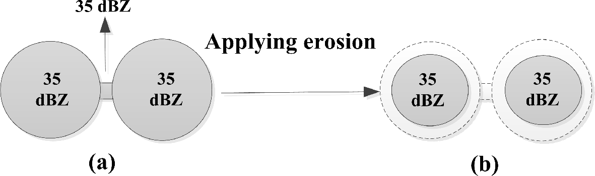
The single threshold systems face three major problems. The first one is choosing a suitable threshold value. If the initial threshold value is too high, storm(s) initiation may not be detected; also, stratiform events may be ignored, and setting it to a low value may result in an unrealistically large storm. The second problem is the weak connection between two or more storms, called false merger, while the third one is the inability of identifying sub-storms within a cluster of storms. 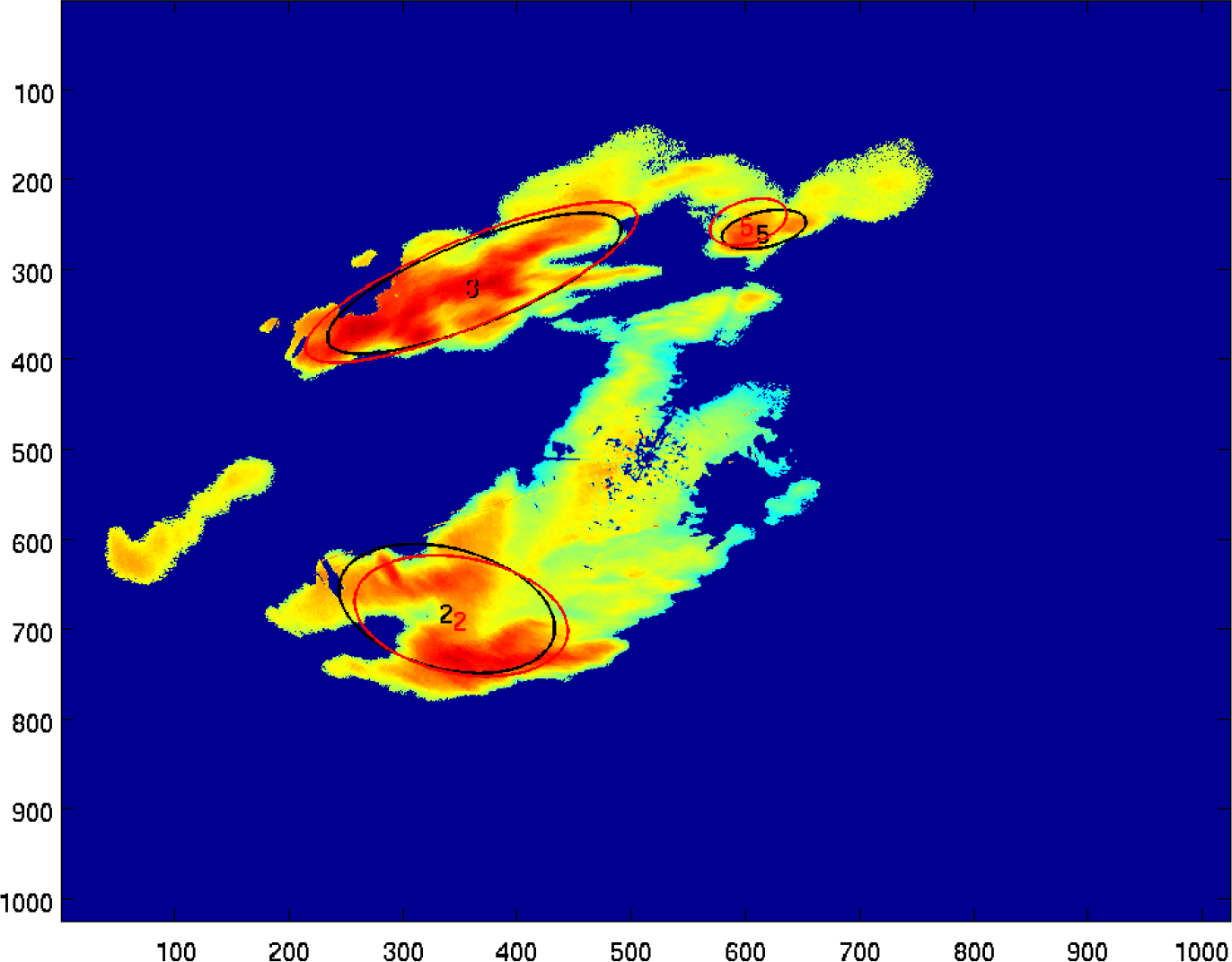In the case of false merger, the identification algorithm falsely treated these loosely connected storms as a single (merged) storm (see Figure 1). Clusters of storms can be defined as a large storm that has further strong reflectivity sub-storms (see Figure 2).

To overcome the problem of choosing a suitable initial threshold value, we have proposed fully-automated thresholding techniques (discussed in Sections 3.1.1 and 3.1.2) based on ThreshGW (G stands for Gonzalez and W for Woods) [9] and graythresh [10]. The false-merger problem is solved by using mathematical morphology (given in Section 3.3), particularly morphological erosion, discussed in [9]. A multi-level thresholding technique, discussed in Section 3.4, is used to overcome the problem of identifying sub-storms within a cluster of storm(s). Unlike [8], we did not discard any identified storm; also, we did not iteratively dilate (expand) the identified storms to maintain the original structure, like in [6,7].

A track can be defined as the path followed by a storm during its complete life time or from its initiation to the last time it was observed. The storm tracking can be defined as the time association of storms identified at time instance t to the storms already identified and tracked at time instance t-1. Storm(s) splitting, merging, initiation and disappearance make tracking difficult. Storm tracking is discussed in detail in Section 4. Tracking algorithms can be divided into two main categories, i.e., centroid based [4,5,8,11,12] and those which are based on cross-correlation [13–17]. Both techniques have benefits and drawbacks. Centroid-based algorithms can track individual storms more adequately and can provide more information about individual storms. In these algorithms, the center of mass (centroid) of storms is used for tracking. Two storms in two consecutive time instances nearest to each other are candidates for matching. Meanwhile, those algorithms that are based on the cross-correlation produce more accurate speed and direction information for large areas [8]. The hybrid of these two categories was developed by [7,18].

Our proposed procedure is called the combinational optimization technique, because the centroid is used with additional storm attributes for tracking. The centroid-based algorithms proposed until now do not use the reflectivity/precipitation distribution of storms for tracking. In our structure, the amplitude, location, eccentricity difference and areal difference (SALdEdA) variables, we have used the reflectivity and shape information of a storm for tracking. The basic idea behind mapping (associating) two objects of two consecutive time instances is to find how similar they are in structure, amplitude, circularity and area and how closely these storms are located. A global cost function (presented in Section 4.2) is formulated. At this stage, the problem of associating two storms becomes a combinatorial optimization problem. The aim is to find a matching where the global cost function is minimized. Hungarian (see [19]) is the candidate algorithm for solving our problem, because it is relatively easy to implement.

Section 5 discusses storm forecasting. Forecasting is the prediction of future event(s). Our variables of interest for forecasting are the area of the storm, the major/minor axis length, the angle of orientation, the speed and the direction. We have adopted first and second order exponential smoothing strategies in order to model our variables of interest.

2. State-of-the-Art

As mentioned before, most of the early attempts for storm identification were threshold based. A few examples are discussed in this section.

The original TITAN, discussed in [4], uses a single reflectivity threshold to identify the storm(s). The updated version of TITAN uses two reflectivity thresholds to overcome the problem of false-mergers. TITAN defines storms as a contiguous region exceeding thresholds for both reflectivity and volume. The identification procedure consists of two steps: first, the identification of contiguous sequences of points (called run) for which the reflectivity exceeds T_z (minimum threshold value in dBZ); second, the grouping of all runs that are adjacent. Storms with volumes less than volumetric threshold T_v are dropped. TITAN calculates storm properties, such as centroid, vertically-integrated liquid (VIL), volume, etc. TITAN is unable to identify storm cells within a cluster of storms. Beside this, if the reflectivity threshold is kept high, TITAN is not capable of identifying storm initiation and also stratiform events.

SCIT (the storm cell identification and tracking algorithm) is another algorithm that processes volumetric reflectivity information by using a multi-level thresholding technique [8]. SCIT uses a predefined list of seven different reflectivity thresholds, i.e., 60, 55, 50, 45, 40, 35 and 30 dBZ. Identification of storms is carried out in different stages, starting from 1D (one-dimensional) data processing, called a run, similar to TITAN. All runs are then combined into 2D storm components. Though SCIT has the strength to identify the storm cells within a cluster of storms, yet is unable to detect storm initiation or storms with a reflectivity less than 30 dBZ, consequently, it drops the storms identified by lower threshold values, which may be interesting for some users. Both TITAN and SCIT face the problem of false merger isolation.

ETITAN (enhanced TITAN) was developed by [7]. The storm identification step is based on TITAN and SCIT with some additional features. Identification of the run and grouping the adjacent runs is similar to TITAN. ETITAN has the capability to identify sub-storms within a cluster of storms using the seven reflectivity thresholds as used by SCIT. In order to cope with the problem of false mergers, ETITAN has introduced mathematical morphology. SCIT dilates (expands) storms iteratively to maintain the internal storm’s structure. ETITAN has a similar built-in problem as SCIT, such as its inability to detect storm(s) initiation or storms with lower reflectivity.

As mentioned earlier, storm tracking algorithms are mainly classified into two classes, i.e., centroid based [4,5,8,11,12] and correlation based [13–17] algorithms. These approaches have been reviewed in [20], while [21] discusses the comparison of nine nowcasting tools deployed during the Olympic Games 2000, Sydney, Australia, under the umbrella of WWRP (World Weather Research Programme).

TITAN tracks the storms using a combinatorial optimization procedure [4]. A cost is calculated for every pair of storms in t and t-1, which is the weighted sum of the distance between the centroids of the storms and the difference in their volumes. A true set of tracks that minimizes the cost function is found.

The storm cell identification and tracking (SCIT) discussed by [8] identifies storm cells in two successive radar scans and temporally associates the identified cells to find the track of every cell. The time difference between two consecutive radar scans is determined. If the time difference is greater than a certain time interval (20 min), discontinuity is recorded. Centroids of cells at time t-1 are projected as a first estimate for the locations of cells in current time t-1 based on time instances t-k, where k > 1. Every cell of time t is associated with the closest cell in a searching radius. If there is no cell in the searching circle, it is considered as a new cell.

The effective evaluation of tracking has not been explored very much by researchers. Johnson et al. [8] introduced a simple, but labor-intensive procedure for the tracking evaluation called “percentage correct”. It is simply the ratio of correctly-tracked storms and total tracks. Lakshmanan and Smith [22] proposed the following set of metrics based on statistics for each track:

• Dur is the total life time (duration) of a track;
• The standard deviation of VIL (σ_v);
• The root mean square error of centroid positions from their optimal line fit.

The atmosphere cannot be predicted perfectly in a certain way, because of its non-linearity. According to Bellon et al. [23], the main reasons for the loss in forecast skill are not due to errors in the forecast motion; rather, they are due to the unpredictable nature of the storms in terms of growth and decay. Therefore, statistical methods for forecasting are the essential part of forecasting tools [24]. The most widely-used technique for weather forecasting is linear or least squares regression [24]. Lu et al. [25] presented a weather predicting system based on a neural network and fuzzy inference system, which is out of scope of the current work. TITAN assumes the decay and growth of storms follow a linear trend, while storm motion occurs along a straight line. A linear regression model, called double exponential smoothing, is adopted for linear trend modeling of the variables of interest [4].

Forecast evaluation or validation and verification are the processes of assessing the quality of forecasts. Various kinds of forecasts validation techniques exist, where the basic criterion is to compare the forecasts with the original observations. The definition of a good forecast is subjective, but generally speaking, a forecast is good if the difference between forecasts and the original observations is small. The famous technique for forecasts evaluation is the contingency table approach [26] used by [3,4,7].

3. Storm Identification

The storm/cell is the experimental unit and is respectively defined as a contiguous region with reflectivity and area above T_z and T_a. Storm identification is the recognition of individual storms’ boundaries and computes their characteristics, i.e., centroids, area, major/minor radii and orientation, etc. Most of the storm-based weather forecasting systems use a thresholding technique for the identification of storms/cells.

After identifying storm(s), we calculate the area of the storm(s) by counting the number of pixels in the storm(s), and then, we apply the areal threshold value, i.e., T_a. The qualifying storm(s) is subjected to further processing. Storms approximated by ellipses and attributes, like the centroid, major/minor axis orientation, etc., are calculated according to the procedure discussed in [27].

3.1. Thresholding

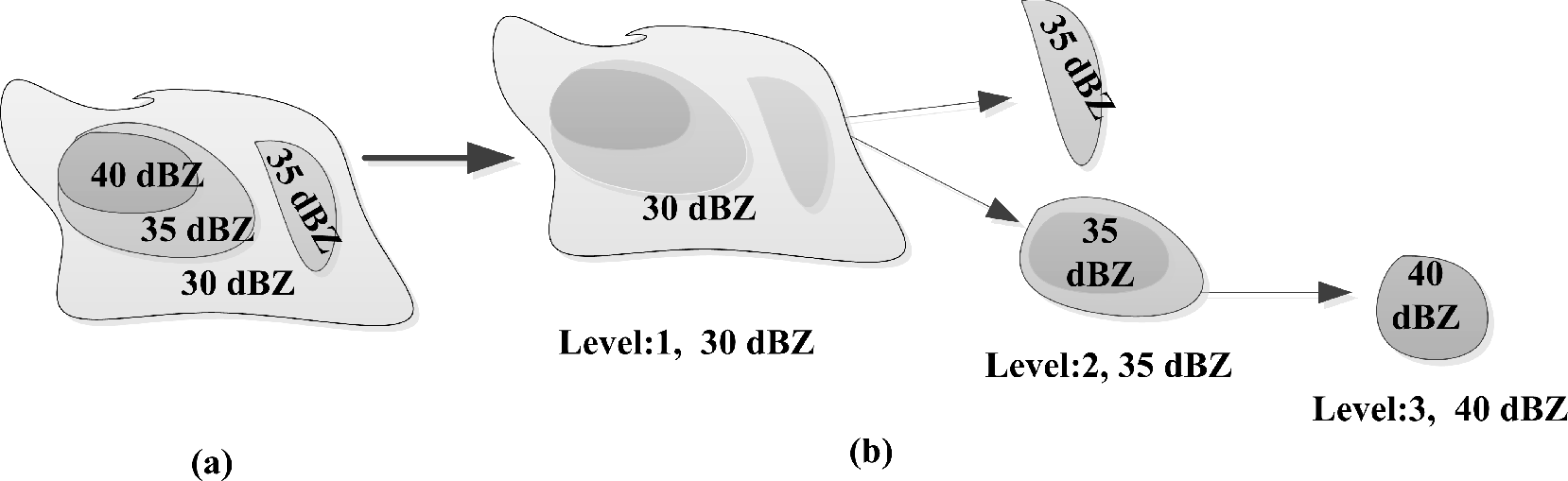
Single thresholding divides an image into two classes, i.e., background class (C₀) and foreground class (C₁). In the case of radar images, radar echoes are the foreground, while their absence is the background of the image. Since we are interested in rain, pixels belonging to C₀ are dropped, while pixels belonging to C₁ are kept for further processing. A single threshold only separates the background from the foreground, but it is not capable of identifying different objects (storms/cells) in the foreground. The foreground after applying a single threshold is called a cluster if it has sub-storms, as shown in Figure 2. To correctly separate the sub-storms of a cluster, multi-level thresholding, also called multi-thresholding, is required. Most of the weather forecasting systems have left the choice of selecting the initial threshold to the users of the system. Normally, the user performs some trial and error to choose the appropriate threshold. Our aim is to develop a fully-automated system capable of calculating a suitable initial threshold value and also to find out the number of appropriate levels. Many techniques have been developed for threshold calculation, such as histogram-, clustering- and entropy-based methods. Some of these techniques are parametrized and/or supervised, while others are non-parametric and unsupervised methods. We have selected two methods, which are ThresholdGW [9] and graythresh [10], which are totally automated, non-parametric and unsupervised procedures. The first method is not popular, but is easy to implement, while the second one is popular in the image processing community. These methods calculate the initial threshold in the grey scale, which is then converted into radar reflectivities. Our system also supports single thresholding and semi-automatic multi-level thresholding.

3.1.1. ThresholdGW

Gonzalez and Woods [9] describe an iterative procedure for automatic threshold selection. We named it ThresholdGW. An initial estimate for T_z is calculated as the average of the maximum and minimum intensities in the radar image. The image is segmented into two classes, i.e., C₀ and C₁, using T_z. The mean T_z is calculated for each class, and the final T_z is the average of the mean of the background and foreground.

3.1.2. Graythresh

The basic idea of graythresh is to divide image data into C₀ and C₁ on such a point that maximizes the variance between the background and foreground classes, called between class variance ${\sigma }_B^2$. The histogram of a gray scale image is computed where each bin corresponds to each gray level from zero to 255. Each gray level is considered as a dividing point for which the between class variance is computed. Finally, a gray level with maximum ${\sigma }_B^2$ is selected as T_z. The detailed procedure is given in [10].

3.2. Storm Labeling

After applying thresholding, the next step is to group the qualifying pixels into different storms. The technique used for grouping together relevant pixels in different storms is called labeling. We start from the top left corner of the image and search for the first non-zero pixel, say p, at coordinate (x, y), and we label it as one. Now, the rest of the pixels can be connected to p by using two different adjacency criteria [9]. A pixel p can have two horizontal and two vertical neighbors, according to the four-neighbors adjacency method, which can be represented by N₄ (p), while p also has its four diagonal neighbors, which can be represented by N_D (p). The union of N₄ (p) and N_D (p) results in the eight-neighbors adjacency method, which can be represented by N₈ (p).

Pixels p and q are said to be four-adjacent if q is one and q ∈ N₄ (p). Furthermore, p and q are said to be eight-adjacent if q is one and q ∈ N₈ (p). If p and q are conned pixels, q is labeled as p. When a new unconnected pixel p is found, the storm label is incremented by one, and so on. Pixels having the same label belong to the same storm. The value of the label represents the storm the number.

Though we have implemented both N₄ (p) and N₈ (p), we recommend using only N₄ (p), because N₈ (p) increases the probability of false mergers.

3.3. Mathematical Morphology

Morphological operations typically probe an image with a small shape or template, known as the convolution mask or structuring element (SE). SE controls the manner and extent of the morphological operation [9].

We are interested in erosion, which shrinks or thins the objects depending on SE. The erosion of image I by structuring element B, denoted by I ⊖ B, is defined as:

$$I\ominus B=\left\{x\right|{(B)}_x\subseteq I\}$$

(1)

The erosion of I by B is the set of all points x, such that B is translated by x contained in I. As shown in Figure 1, Figure 1a is the original image I, while Figure 1b is the resultant image after erosion.

3.4. Multi-Level Thresholding

As mentioned before, a single threshold cannot isolate sub-storms of a cluster. After calculating the initial threshold value, higher levels are computed by successively adding a certain integer value to the previous level until the maximum reflectivity value is reached. The thresholding technique discussed before is applied for every threshold’s level.

4. Storm Tracking

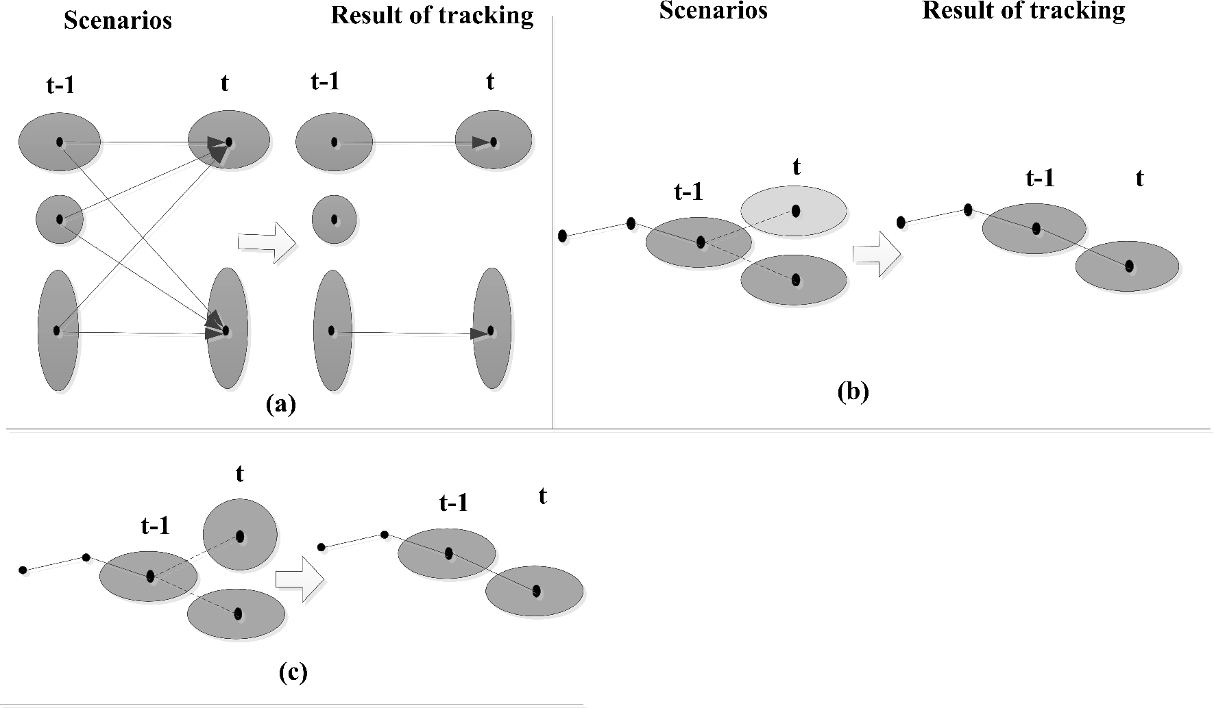
Generally, centroid-based approaches use the center of mass for tracking, while some of them use area, as well, i.e., TITAN, ETITAN (enhanced TITAN). TITAN further improved its tracking procedure by introducing optical flow [28]. These approaches can easily track the situation, as shown in Figure 3a, but they cannot correctly track the storms shown in Figure 3b,c. Figure 3b shows that the candidate storms at t have the same area and the same distance from storms at t-1, but a different reflectivity distribution. Furthermore, Figure 3c shows that both candidate storms at time t have the same area, the same distance from the center of masses at t-1 and the same reflectivity distribution, but their shape is different, i.e., one is more circular, while the other one is elongated. Having similar assumptions as that of TITAN for tracking, we additionally assume that the reflectivity distribution and the shape of a storm in two successive radar scans do not change abruptly.

The SAL (structure, amplitude and location) method was proposed by [29] for the purpose of the verification of the quantitative precipitation forecasts. The basic idea of SAL was to present an object-based quality measure for the verification of forecasts. Here, a modified version of SAL with some other additional characteristics of storms have been used for tracking.

4.1. Definition of Components of SALdEdA

Consider a domain D_i,t, which represents a storm that is N_i,t pixels large, where i = 1, 2, 3 …n, where n corresponds to the number of storms per radar scan (image/map). The current time is represented by t, while t-1 denotes the previous time instance. The current storm number is represented by i, while the previous one by j, where i = 1,2, …n_t and j = 1,2, …n_t−1. The radar reflectivity of the i-th storm at time t in dBZ is represented by Z_i,t. The maximum reflectivity of a storm is represented by $Z_{i,t}^{max}$. If SALdEdA is used for precipitation objects, Z should be replaced by R.

4.1.1. The Structure Component

The key idea of using the structure component, S, is to compare the volumes of normalized reflectivity objects. Originally, the S component was calculated for multiple precipitation objects, either in original observations or in the forecasts [29], while here, in our case, we calculate S only for two storms at a time belonging to two consecutive time instances. Therefore, here, the S is much more simplified than that of the original S.

$$S_{i,j}=\left|\frac{V_{i,t}-V_{j,t-1}}{V_{i,t}+V_{j,t-1}}\right|;\begin{array}{c}i=1,2\dots n_t\\ j=1,2\dots n_{t-1}\end{array}$$

(2)

where n_t and n_t−1 correspond to the number of storms at t and t-1. S is 0 ≤ S_i,j ≤ 1. S_i,j is equal to zero if two storms are structurally the same, while S_i,j = 1 indicates that the storms have totally different volumes. Volume (V_i,t) is calculated as below:

$$V_{i,t}=\frac{{\displaystyle {\sum }_{(x,y)\in D_{i,t}}{Z}_{x,y}}}{Z_{i,t}^{max}}=\frac{Z_{i,t}}{Z_{i,t}^{max}}$$

(3)

Scaling of Z_i,t with $Z_{i,t}^{max}$ is compulsory in order to distinguish the S component from the A component of SALdEdA. Z_i,t can be calculated as follows:

$$Z_{i,t}={\displaystyle \sum _{(x,y)\in D_{i,t}}{Z}_{x,y}};n=1,2,\dots n_t$$

(4)

Here, Z_x;y is the pixel reflectivity value in dBZ.

4.1.2. The Amplitude Component

This is the normalized, absolute difference of the mean reflectivity of two storms subjected to tracking.

$$A_{i,j}=\left|\frac{M(Z_{i,t})-M(Z_{j,t-1})}{M(Z_{i,t})+M(Z_{j,t-1})}\right|$$

(5)

Here, M(Z_i,t) corresponds to mean reflectivity.

$$M(Z_{i,t})=\frac{1}{N_{i,t}}{\displaystyle \sum _{(x,y)\in D_{i,t}}{Z}_{x,y}}=\frac{Z_{i,t}}{N_{i,t}}$$

(6)

where N_i,t is the total number of pixels in the i-th storm and Z_x,y is the pixel reflectivity value in dBZ. The value of the amplitude (A) is 0 ≤ A_i,t ≤1; where A_i,t = 0 means that the i-th and j-th storms have complete agreement, while A approaching one means full disagreement between the corresponding storms with respect to amplitude. Though, theoretically, the A component can be one, practically, it cannot be, because A = 1 means one of the storms has zero mean reflectivity, which is not possible in our case (reflectivity values greater than zero are only considered).

4.1.3. The Location Component

This is the normalized distance between the centers of mass of two storms. The L component is calculated as:

$$L_{i,t}=\frac{\left|x(Z_{i,t})-x(Z_{j,t-1})\right|}{d}$$

(7)

where d is equal to the diameter of the area that is covered by radar measurements and x(Z_i,t) represents the center of mass of the i-th storm. The value of L_i,j is in the range of [0, 1]. When L_i,j = 0, two storms have exactly the same position, while L_i,j = 1 indicates that the two storms are the boundaries of the radar coverage area separated by distance d. Smaller values of L between two storms at two successive radar maps show that they are candidates for temporal association. Since the center of mass is a single point in a storm, therefore, tracking depending on it could be erroneous. The change in the reflectivity of storms will change its center of mass, even if it is in its old position, thus resulting in the motion of the storm.

4.1.4. The Eccentricity Component

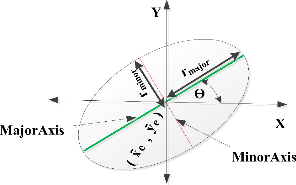
The dE component stands for the difference of eccentricities of two storms subjected to comparison for matching. We assume that the eccentricity of storms does not change abruptly between two consecutive radar images. The eccentricity of an ellipse is a measure of how circular an ellipse is. The eccentricity E of an ellipse given in Figure 4 is calculated from the aspect ratio using Equation (8). TITAN assumes that the aspect ratio $\frac{r_{minor}}{r_{major}}$ of a storm remains constant between two consecutive time intervals.

$$E=1-\frac{r_{minor}}{r_{major}}$$

(8)

$$d{E}_{i,t}=\left|E_{i,t}-E_{j,t-1}\right|$$

(9)

The absolute difference of eccentricities lies in the range of [0, 1], where dE_i,j = 0 means that both storms have the same eccentricity, while dE_i,j = 1 shows that one of the storms is perfectly circular, while the other one is a perfect line.

4.1.5. The Area Component

The area of a storm is the total number of pixels in it. We have used the normalized, absolute areal difference to calculate dA. The key idea for tracking is that two storms are candidates for matching if the difference in their areas is minimum.

$$d{A}_{i,j}=\left|\frac{Are{a}_{i,t}-Are{a}_{j,t-1}}{Are{a}_{i,t}+Are{a}_{j,t-1}}\right|$$

(10)

dA_i,j ranges in [0, 1]. Practically, dA cannot be equal to one, because the area of a storm cannot be zero.

4.2. Objective Function

The objective Function Q is defined as:

$$Q={\displaystyle \sum C_{i,j}}$$

(11)

where C_i,j is the cost when the i-th storm of the t time instance is compared with the j-th storm of t-1. C_i,j is defined as:

$$C_{i,j}=w_1{S}_{i,j}+w_2{A}_{i,j}+w_3{L}_{i,j}+w_{4}d{E}_{i,j}+w_{5}d{A}_{i,j}$$

(12)

where w_i is in the range of [0, 1]. The combinatorial optimization problem is solved by using the Hungarian algorithm [19].

Some restrictions are imposed to control the scope of the feasible solution set. For example, TITAN puts a restriction over the speed L/Δt of a storm that should be less than a certain maximum speed; otherwise, the association is not considered feasible for tracking. However, it is not a robust method, because it fails for different sizes of storms. Shah et al. [30] adopted a procedure that compares the distance between the center of masses of the two storms with MAXDISTaccording to the size of the storm at t-1, but it covers only six situations. If the size of the storm changes, the value of MAXDIST also changes. In this work, we have adopted a more robust and flexible procedure by putting a limitation over the distance (L) between two candidate storms. Only those matching are considered feasible if the distance (location (L) component) between the two candidate storms is less than $\frac{\alpha .MajorAxis}{d}$, where d is the diameter of the radar’s coverage circular area and α ranges between zero and one, which further controls $\frac{MajorAxis}{d}$.

4.3. Handling Splits and Mergers

Storm merging occurs more frequently while splits occur less frequently [4]. When a merger occurs, the best matching track is extended, while the others are terminated. In the case of a split, the best match is extended, while the rest are treated as new initiated storms.

5. Storm Forecasting

Forecasting is based on the identification, modeling and extrapolation of patterns found in the time series of data. These patterns include the linear trend, cyclic trend, seasonal behavior and randomness in data. In order to model a time series, we have to remember a few notations. T represents the current time; τ represents the forecast leading time; t is the iterating variable; y_T represents the original observation at time T; ${\tilde{y}}_T$ represents the fitted value of y_T ; and ŷ_T represents the forecasted value at T. Let us suppose that p_T is the current value of a parameter pand that $\frac{dp}{Dt}$ is the temporal derivative, then:

$$p_{T+\tau }=p_T+\left(\frac{dp}{Dt}\right)\tau$$

(13)

Our variables of interest for the forecasting are the area of the storm, major/minor axis length, angle of orientation and speed and direction. We have adopted first order and second order exponential smoothing strategies in order to model the above time series. The forecast of these variables is based on the assumption that the growth and decay (increase and decrease) of these variables are linear. Exponential smoothing is a technique that assigns geometrically decreasing weights to the previous observations [31]. In order to start the process, we set ${\tilde{y}}_0=y_0$. First and second order exponential smoothing are calculated as:

$${\tilde{y}}_T^{(1)}=\lambda y_T+(1-\lambda ){\tilde{y}}_{T-1}$$

(14)

$${\tilde{y}}_T^{(2)}=\lambda {\tilde{y}}_T^{(1)}+(1-\lambda ){\tilde{y}}_{T-1}^{(2)}$$

(15)

where ${\tilde{y}}_T^{(1)}$ and ${\tilde{y}}_T^{(2)}$ are the first and second order exponential smoothers. Furthermore, note that 0 ≤ λ ≤ 1. Higher values of λ provide less smoothing, and the smoothed observations follow the original observations, while smaller values of λ provide more smoothing. In the former case, more focus is given to the latest observation, while in the latter case, historical observations are also considered. The recommended value of λ in the literature is between 0.2 and 0.4 [31]. We have adopted an automated, but modified procedure for choosing a suitable value of λ discussed in [31].

5.1. Forecasting

At time T (current time), someone may want to forecast the observations into the next time period T + 1 or even further in the future T + τ. The forecast at T + 1 is called one-step, while at T + τ is called τ-step ahead forecasting.

The line trend assumes that the growth or decay in the variable of interest is linear in nature. The τ-step ahead forecast for the linear trend model can be formulated as follows:

$${\widehat{y}}_{T+\tau }(T)=\left(2+\frac{\lambda }{1-\lambda }\tau \right){\tilde{y}}_T^{(1)}-\left(1+\frac{\lambda }{1-\lambda }\tau \right){\tilde{y}}_T^{(2)}$$

(16)

where ${\tilde{y}}_T^{(1)}$ and ${\tilde{y}}_T^{(2)}$ are the first and second order exponential smoothers at time T (current time).

5.2. Choosing λ

A list of values, i.e., {0.1, 0.2, 0.3, 0.4, 0.5, 0.6, 0.7, 0.8 and 0.9}, for λ is chosen. For each value of λ, the MSE (mean squared error) is calculated, and the value that gives the least MSE is picked for λ. MSE is defined as:

$$MSE(\lambda )=\frac{1}{T}{\displaystyle \sum _{t=1}^T{e}_{t-1}^2(1)}$$

(17)

where $e_{t-1}^2(1)$ is the one-step-ahead forecast error. The forecasting error is calculated as:

$$e_T^2={(y_{T+1}-{\tilde{y}}_{T+1}(T))}^2$$

(18)

6. Results

The results have been produced to testify to the efficiency and goodness of the system using datasets collected from two radar sites, i.e., Turin and Foggia. See Section 6.1 for further details about the description of the datasets. The multi-threshold procedure is adopted only for storm identification; for storm tracking and forecasting, the single threshold criterion is used for simplicity. Since the system consists of three major steps, results are also presented section wise. Morphological erosion is set to on with the exception of those cases where a comparison is required between on/off. A 3 × 3 structuring element (SE) or convolution mask for the erosion is used. For storm labeling, the four-neighbor adjacency method is used. The eight-neighbor adjacency criterion is avoided, because its only difference from that of four-adjacency is close to the boundaries where the boundaries are shrunken by erosion, nullifying its effect. The multi-level threshold for multi-level storm identification is separated by 5 dBZ. As mentioned earlier, the identified storms are approximated by ellipses. The color scheme for the ellipse’s boundary with respect to threshold value in dBZ is: {red:15, white:20, magenta:25, green:30, black:35, blue:40, cyan:45 and yellow:50 dBZ}. For storm tracking and forecasting, the color scheme of the ellipse’s boundary is: {white:history, black:current and red:forecast}. All of the displayed storm’s images are in dBZ. The areal threshold T_a is set to 10 km² for all experiments.

6.1. Dataset Descriptions

Davini et al. [32] performed a radar-based analysis of convective events over northwestern Italy, while we have collected datasets from two radar sites, i.e., Turin and Foggia. Both convective and stratiform events have been taken into account, as shown in

Table 1. Selected datasets; F = Foggia, T = Turin, C = convective, S= stratiform and DID = dataset ID.

DID	Events	Start Time	End Time	Duration (Minutes)
	Foggia
FC1	1 April 2013	16:31:04	20:00:04	210
FC2	2 and 3 April 2013	19:00:05	03:00:06	481
FC3	27 April 2013	04:20:05	13:20:05	541
FC4	2 May 2013	05:21:04	08:00:04	161
FC5	3 June 2013	10:00:06	13:00:06	181
FC6	9 August 2013	15:30:04	22:30:05	403
FC7	20 August 2013	11:00:05	18:20:05	290
FC8	22 August 2013	13:31:05	12:50:04	111
FS1	25 November 2013	04:21:06	09:20:06	300
FS2	27 December 2013	00:01:06	08:00:03	480
	Turin
FC9	23 and 24 April 2013	23:51:05	03:20:04	210
FC10	8 August 2013	17:01:04	20:40:04	210
FS3	19 December 2013	07:00:03	19:59:04	450
FS4	10 February 2013	12:30:05	15:19:05	500

. The typical western Alps spring and summer time events are mostly convective, while autumn and winter time events are mostly stratiform in nature. For each event, the starting and ending time are specified along with the duration in minutes. In some cases, the starting and ending time do not match with the mentioned duration, because of missing data. Every event has a DID (dataset ID) for reference.

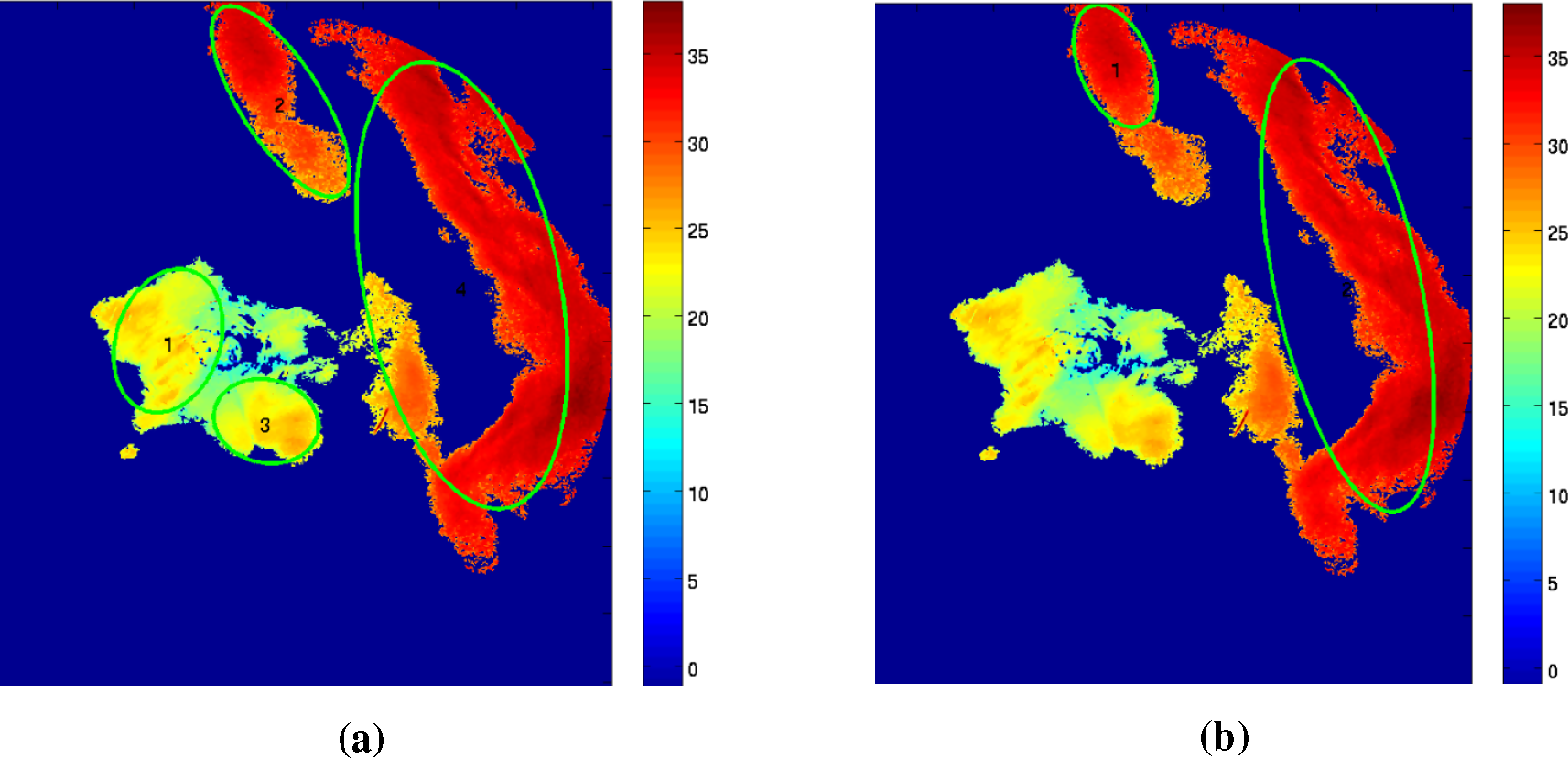
6.2. Automatic Storm Identification

Automatic thresholding solves the first problem of choosing a suitable initial threshold. See Figure 5. Manual threshold selection (Figure 5b) is not able to identify Storms 1 and 3, which are identified by both of the proposed automatic thresholding methods (see Figure 5a). Storms 1 and 3 are at their initiation stage, having low radar reflectivity than randomly chosen T_z.

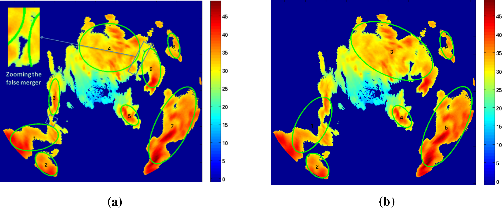
The false merger problem is solved by using morphological erosion. See Figure 6, where the weak connection enclosed by a rectangle in Figure 6a has been broken and the arrow points to the zoomed false merger point. When morphological erosion was switched off, the system was not able to break the weak connection; see Figure 6b.

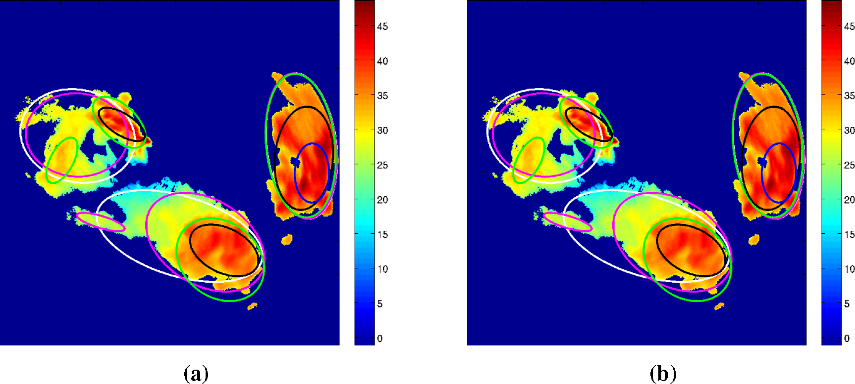
Sub-storms of high reflectivity within a cluster of storms are identified using the multi-threshold technique (see Figure 7). The initial threshold T_z is calculated by graythresh and ThreshGW, and every level has a 5-dBZ reflectivity difference.

6.2.1. Storm Identification Evaluation

Image segmentation is the fundamental process in storm identification; therefore, the quality of storm identification depends directly on the quality of image segmentation. It is a hard problem to design a good quality measure for segmentation [33]. Haralick and Shapiro [34] proposed criteria for good segmentation according to which intra-object homogeneity, inter-object disparity and objects without holes are required.

Intra-object homogeneity is achieved by calculating the within-class variance ${\sigma }_W^2$ as given in [10]. The second point is achieved by computing the between-class variance ${\sigma }_B^2$. The value of ${\sigma }_W^2$ is expected to be small, while the value of ${\sigma }_B^2$ is expected to be large. The lack of holes is checked by human eyes. Otsu [10] evaluated the “goodness” (measures of class separability denoted by η) of the threshold by using the following discriminant criterion measures.

$$K=\frac{{\sigma }_W^2}{{\sigma }_T^2},\eta =\frac{{\sigma }_B^2}{{\sigma }_T^2}$$

(19)

where ${\sigma }_T^2$ is the total variance of an image. A good quality threshold yields smaller K and larger η. The values of both K and η ranges between zero and one, i.e., 0 ≤ {K, η} ≤1. η = 0 and K = 1, if the image has a single constant grey level, while η = 1 and K = 0 if the image has only two values (binary image). Our aim is to obtain η close to one and K close to zero.

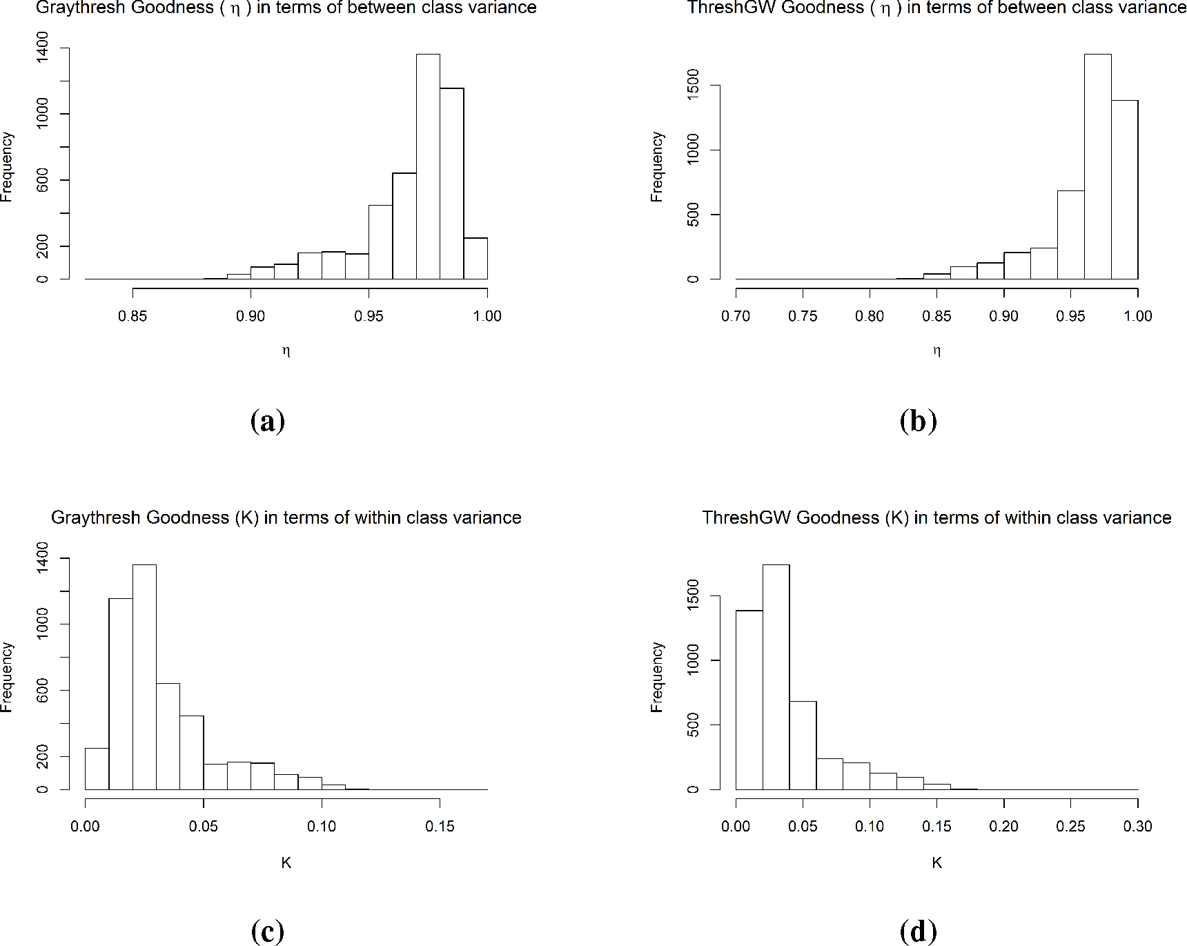
The obtained results given in

Table 2. Storm identification evaluation; mean values of η, K, ω₀ and ω₁ are given in the form of graythresh/ThreshGW up to 4 decimal places.

	η	K	ω0	ω1
Foggia	0.9770/0.9720	0.0233/0.0279	0.8395/0.8407	0.1605/0.1592
Turin	0.9478/0.9386	0.0522/0.0614	0.8915/0.8950	0.1085/0.1050
Overall	0.9681/0.9619	0.0318/0.0381	0.8553/0.8572	0.1447/0.1427

and Figure 8 show that both graythresh and ThreshGW produced good results for η and K for all datasets with 97% goodness. The values of ω₀ and ω₁ (respective probabilities of the background class C₀ and the foreground class C₁) show that even in rainy radar images, 85% of the image is occupied by non-rainy pixels. The results also show that the effects of both thresholding techniques are almost the same for segmenting radar images. Therefore, any one of the two can be used for calculating the initial threshold T_z.

6.3. Storm Tracking

We used T_z = 28 dBZ for the identification of convective and T_z = 20 dBZ for the identification of stratiform events. Our main focus is to find the contribution of each variable of SALdEdA in storm tracking and to evaluate the goodness of the overall system after combining SALdEdA variables for tracking.

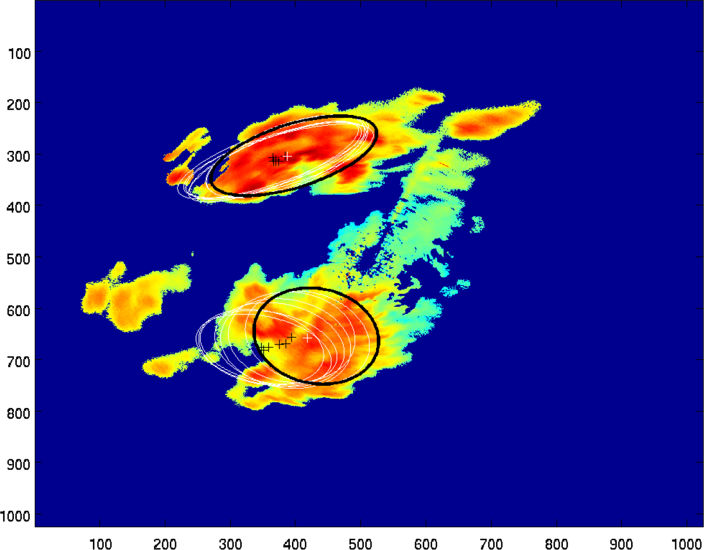
Figure 9 shows two tracks with a seven-minute history represented by white ellipses. The contribution of each variable of SALdEdA in storm tracking is shown in

Table 3. Contribution of structure, amplitude, location, eccentricity difference and areal difference (SALdEdA) variables in storm tracking; the total number of tracks is 683.

Variables	Wrong Tracks	Correct Tracks	Percentage Correct
S	160	523	76.57
A	554	129	18.88
L	485	198	28.99
dE	653	30	4.39
dA	143	540	79.06

. The obtained results show that both the S and dA components play almost similar and significant roles in tracking, while dE plays the least role. On the basis of the results in Table 3, similar weights have been given to S, dA and L, while half to A and a quarter to dE, while computing the cost of Equation (12).

As mentioned in Section 4.2, the matching is not feasible if the distance between the two matching storms is greater than $\frac{\alpha .MajorAxis}{d}$. Experiments have been performed to find the suitable value for α, and the obtained results in

Table 4. “Percentage correct” for different α values, while restricting the searching space.

DID	α1:0	α0:95	α0:90	α0:85	α0:80
Total	61.32	73.64	99.34	78.99	74.93

show that for α= 0.90, the best results are achieved. “Percentage correct” is discussed next in Section 6.3.1.

6.3.1. Tracking Evaluation

The evaluation procedure adopted in this work is called “percentage correct” [8]. For this method, the ratio of the number of correct tracks labeled by our method to the total number of tracks labeled by a human is calculated. The “percentage correct” is computed by manually comparing the output of our tracker with human-labeled associations. One of its serious flaws is its labor intensiveness.

Possible tracking errors are shown schematically in Figure 10, where dotted lines represent the expected correct tracking and the arrow lines show the incorrect tracking. The missed association is shown in Figure 10a, where the tracking algorithm was expected to continue the track, but the tracking is terminated at t₃ and a new track is started at t₄. A wrong association is depicted in Figure 10b,c. The fault of Figure 10c is due to the wrong threshold value of the maximum distance between them.

The overall performances of our tracking procedure have been compared with manually-tracked storms. The obtained results, given in

Table 5. Tracking evaluation of our procedure for all datasets.

DID	Total Tracks	Wrong Tracks	Correct Tracks	Percentage Correct
FC1	42	0	42	100
FC2	44	0	44	100
FC3	123	3	120	97.560
FC4	36	0	36	100
FC5	38	0	38	100
FC6	90	2	88	97.77
FC7	83	0	83	100
FC8	17	0	7	100
FS1	18	0	18	100
FS2	67	0	67	100
FC9	22	1	21	95.45
FC10	60	0	60	100
FS3	30	0	30	100
FS4	23	0	23	100
Total	683	6	677	99.34

, show the significance of our procedure with 99.34% accuracy. The obtained results also show that 100% accuracy has been achieved for stratiform events, because of the static nature of these storms.

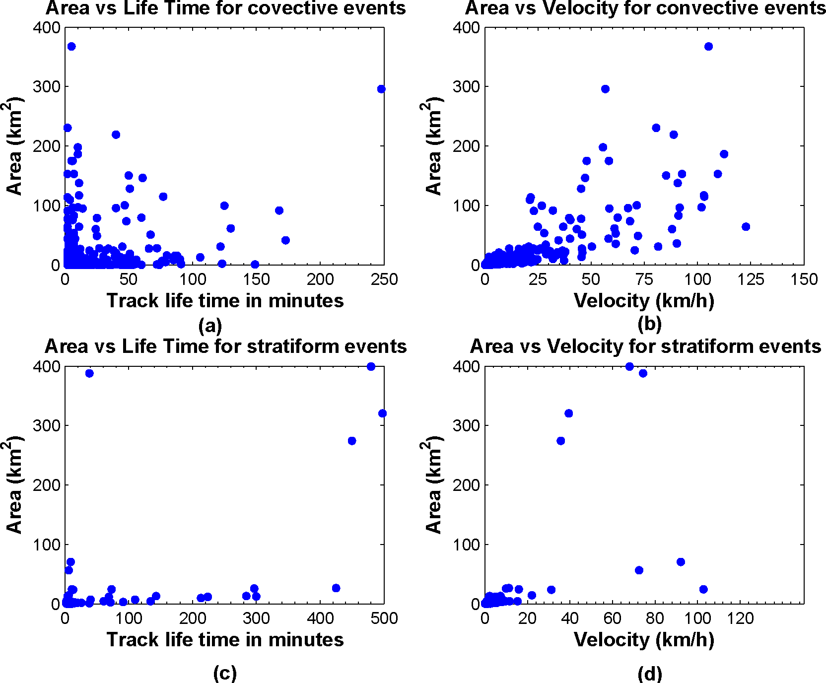
The scatter plot in Figure 11 shows the relationship between the storm’s life time and its area and between the velocity and area for both convective and stratiform events. Figure 12b shows that most of the storms span up to one hour. Figures 11 and 12a reveal that most of the convective storms have less than a 30-km² area with a velocity up to 50 km/h. For the convective storms, the life time may not be the actual one, because a storm can originate outside the of coverage area of our radar; therefore, the tracking in this case may be partial.

A similar analysis has been performed for stratiform events in Figures 11 and 12c,d. The obtained results show that stratiform storms span more than convective storms.

6.4. Forecasting

In order to forecast variables of interest, the forecast leading time (FLT) has been set to 5, 10 and 15 min. The minimum history required for forecasting is set to 3 min. A five-minute forecast with corresponding current storms is shown in Figure 13.

As mentioned in Section 5, all of the variables of interest are forecasted using the second order exponential smoothing technique. To choose a suitable value for λ in Equations (14) and (15), an automated criterion is adopted. Higher values of λ provide less smoothing, and the modeled values closely follow the original observation, while lower values for λ provide more smoothing. Figure 14 shows that the value of λ is mostly around 0.50 ± 0.02 on average. The results are quite acceptable for balancing smoothness and following the original observations.

6.4.1. Forecasting Evaluation

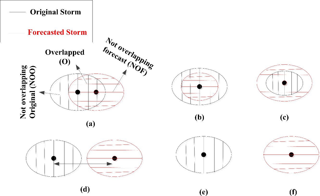
Many factors contribute to the QPF (quantitative precipitation forecast) error, including location and intensity errors. A parametric scheme is introduced by Mecklenburg et al. [35] to separate position and intensity errors. Further details about forecast verification can be studied in [36]. Some possible cases of forecasts with current storms have been shown in Figure 15. In most cases, the forecast and current storm overlap each other, but in some cases, as depicted in Figure 15d,e,f, the forecast and current storm may not overlap each other or one of them is missed. A contingency table is used to evaluate the accuracy of forecasts.

A “hit” occurs if the overlapped (O) area is greater than the sum of non-overlapping original (NOO) and non-overlapping forecast (NOF) areas. The rest of the table is filled accordingly if the above condition is false. An “underestimate” is recorded if O ≠ 0 and C (current area) is greater than the F (forecasted area). An “overestimate” is counted if F is greater than C and O ≠ 0. A “missed event” describes the case when there is no forecast for the current storm, as depicted in Figure 15e. If both the current storm and forecasted one do not overlap each other, a “missed location” is counted, as shown in Figure 15d. In the case of a “missed location”, the amount of rain forecasted may be underestimated, overestimated or reasonably good. A “false alarm” occurs if the forecasted storm has no matching current storm, as shown in Figure 15f.

The obtained results are presented in

Table 6. Forecast evaluation. FLT, forecast leading time. All measures are shown as a percentage.

FLT	Underestimate	Hits	Overestimate	Missed Event	Missed Location	False Alarm
Convective Events
5	2.11	89.95	1.16	6.77	0	0
10	4.06	84.36	4.49	7.07	0	0
15	6.38	78.64	8.26	6.70	0	0
Stratiform Events
5	1.63	91.34	0.86	6.16	0	0
10	2.64	88.47	1.78	7.09	0	0
15	4.29	85.68	2.96	7.05	0	0

showing the positive forecasting capabilities of our system. For the stratiform events, a performance increase is noted exactly according to the expectation, because slower and persistent storms can be more easily detected than highly dynamic convective storms. By increasing the forecast leading time (FLT), a slight reduction of the hit rate is experienced, but still, the “hit” rate is good enough for operational needs. The zero “missed location” shows the accuracy of predicting the speed and direction of the system. The “missed event” rate is a bit high, but still acceptable for operational requirements in comparison to the high “hit” rate. Over- and under-estimation of the area happens rarely. Zero “false alarm” means that the decay of the storms is perfectly predicted, while “missed events” show an early decay in the storm area.

Another contingency table is calculated for comparing the actual mean reflectivity (AMR) with the corresponding forecasted mean reflectivity (FMR). A “hit” is considered if both AMR and FMR existed and the relative difference between the AMR and FMR is within the range of ±0.05, while for less than −0.05, an “underestimate” is recorded, and for greater than 0.05, an “overestimate” is counted. A “false alarm” occurred if either the AMR or FMR is missing.

The results presented in

Table 7. Forecast evaluation for reflectivity estimation. All measures shown as a percentage.

FLT	Hits	Overestimate	Underestimatez	False Alarm
Convective Events
5	88.09	6.89	3.23	1.78
10	78.43	14.56	4.95	2.04
15	68.42	17.49	9.98	4.10
Stratiform Events
5	97.66	1.04	0.66	0.62
10	93.71	2.89	2.56	0.82
15	88.84	5.29	5.08	0.77

show almost a similar trend as that of Table 6. Better performance is noted for stratiform events, while a slight decrease is observed with increasing forecast leading time. A “false alarm” is experienced, because in this table, it combines the missing AMR or FMR.

Finally, it is concluded from the results of Tables 6 and 7 that our system is capable of predicting the area, speed, direction and mean reflectivity of storms.

7. Conclusions

Short-range radars, such as X-band, are quite efficient for monitoring localized rain fall events [37]. Rain data collected from MicroRadarNet^® presented in [2,3] is used in this investigation. Procedures for all major steps, i.e., storm identification, tracking and nowcasting, of a rain nowcasting system have been developed.

Two automatic methods for threshold selection have been tested for storm identification. Each technique is based on the histogram of the image. Inter- and intra-class variances have been calculated to find the goodness of each automatic threshold technique. The problem of “false merger” has been tackled by using morphological erosion, which shrinks the objects (storms). Sub-storms within large storms have been identified using a multi-threshold technique. Storm identification is evaluated for the first time.

A novel procedure, called SALdEdA (structure, amplitude, location, eccentricity (circularity) difference and areal difference), has been proposed for storm tracking. Each component of SALdEdA is computed as the normalized difference between volumes, the mean of reflectivity/precipitation, locations, the eccentricities and areas of storms. A global cost function is formulated as the weighted sum of all of these variables. The combinatorial optimization problem is then solved by using the Hungarian algorithm. The contribution of each component of SALdEdA has been assessed, and recommendations have been given to assign suitable weights to each component, while computing the cost function. The range of the possible solution set is constrained further by limiting the distance between the center of masses of the two matching storms by introducing a flexible procedure. The “percent correct” techniques is used for performance evaluation.

A second order exponential smoothing strategy is used. Two contingency tables have been computed to evaluate the accuracy of forecasting. Predicting storm speed, direction and mean reflectivity was a key aspect for the forecasting evaluation.

In the future, the performance of our system will be compared with already developed tools, such as TITAN [4]. The recently-developed object-based verification method SAL (structure, amplitude and location) discussed in [29] will be used to more accurately evaluate the performance of the system.