
Drought Forecasting Using Stochastic Models in a Hyper-Arid Climate

1
Department of Agricultural Engineering, King Saud University, Riyadh 11451, Saudi Arabia
2
Department of Agricultural Engineering, Ain Shams University, Cairo 11241, Egypt
3
Alamoudi Water Research Chair, King Saud University, Riyadh 11451, Saudi Arabia
*
Author to whom correspondence should be addressed.
Atmosphere 2015, 6(4), 410-430; https://doi.org/10.3390/atmos6040410
Submission received: 1 December 2014
/
Accepted: 11 March 2015
/
Published: 25 March 2015
Abstract
:Drought forecasting plays a crucial role in drought mitigation actions. Thus, this research deals with linear stochastic models (autoregressive integrated moving average (ARIMA)) as a suitable tool to forecast drought. Several ARIMA models are developed for drought forecasting using the Standardized Precipitation Evapotranspiration Index (SPEI) in a hyper-arid climate. The results reveal that all developed ARIMA models demonstrate the potential ability to forecast drought over different time scales. In these models, the p, d, q, P, D and Q values are quite similar for the same SPEI time scale. This is in correspondence with autoregressive (AR) and moving average (MA) parameter estimate values, which are also similar. Therefore, the ARIMA model (1, 1, 0) (2, 0, 1) could be considered as a general model for the Al Qassim region. Meanwhile, the ARIMA model (1, 0, 3) (0, 0, 0) at 3-SPEI and the ARIMA model (1, 1, 1) (2, 0, 1) at 24-SPEI could be generalized for the Hail region. The ARIMA models at the 24-SPEI time scale is the best forecasting models with high R2 (more than 0.9) and lower values of RMSE and MAE, while they are the least forecasting at the 3-SPEI time scale. Accordingly, this study recommends that ARIMA models can be very useful tools for drought forecasting that can help water resource managers and planners to take precautions considering the severity of drought in advance.
1. Introduction
Water demand has significantly increased in many parts of the world, especially in hyper-arid regions that are facing a shortage of available water resources. To make matters worse, world-climatic change is leading to more droughts on the Earth’s surface [1]. Additionally, droughts have always been a normal, recurrent event in arid and semi-arid areas [2]. Floods and droughts projected for the 21st century show large significant changes from those in the 20th century [3]. Prominently, the impact of intense long drought on natural ecosystems essentially concerns regional agriculture, water resources and the environment [4]. The lack of a precise assessment of drought in certain situations may lead to incorrect decisions and actions by managers and policy makers [5]. Therefore, scientists categorized the drought phenomenon into four major groups: meteorological, agricultural, hydrologic and socio-economic [6,7]. These drought categories are usually described using drought detection and monitoring indices, which are based on different natural variables in given time intervals, such as precipitation (PCPN), soil moisture, potential evapotranspiration (PET), vegetation condition, ground water and surface water [8]. In other words, a drought index captures the physical characteristics and their associated impacts.
The most important drought characteristics that may have to be taken into consideration within the index are: the duration, intensity, magnitude and spatial extent of the drought [9]. However, combining these characteristics in one index is extremely difficult. Thus, many researchers have proposed various indices; among these are: the Palmer Drought Severity Index (PDSI) [10], Surface Water Supply Index (SWSI) [11], Palfai Aridity Index (PAI) [12], Standardized Precipitation Index (SPI) [13] and Standardized Precipitation Evapotranspiration Index (SPEI) [14]. In fact, the drought analysis via one of these indices depends on the nature of the index, local conditions, data availability and validity [15].
The pros and cons of the above-mentioned drought indices depend on the simplicity and temporal flexibility of their application. The World Meteorological Organization (WMO) is recommending the SPI as a standard drought index [16]. This is because of the simplicity of its calculations, since precipitation data themselves are sufficient to conduct the test without requiring any statistical complications [17,18,19]. In addition, the SPI could show a high performance in detecting and measuring drought intensity [20]. Despite this convenience, the SPI has still some problems in terms of water balance. Therefore, the SPEI was developed to avoid these problems in the SPI version. The SPEI takes into consideration the sensitivity of PDSI to the changes in PET and the multi-scalar nature of the SPI [21]. The calculation procedure of SPEI is similar to that of SPI [14]. Hence, the difference between the two indices is that the SPEI uses the climatic water balance (the difference between PCPN and PET). The SPEI, therefore, has been used in recent studies as an appropriate index to monitor the drought in many locations of the world [21,22,23,24].
Nowadays, the major challenge in drought research is to develop suitable methods and techniques to predict the onset and termination points of droughts [25]. Hence, the importance of drought forecasting comes from the future mitigation of drought impacts [26]. Several attempts have been made to apply statistical models in hydrologic drought forecasting based on time series methods, such as autoregressive integrated moving average (ARIMA) models, exponential smoothing and neural networks. The ARIMA is a typical statistical analysis model that uses time series data to predict future trends [27]. It can be used in predicting the hydrologic variables, such as: annual and monthly stream flows and precipitation [28]. The ARIMA model approach can outperform most other statistical models, like exponential smoothing and neural network, in hydrologic time series [29]. This relative advantage of the ARIMA model is due to its statistical properties, as well as the well-known methodology in building the model.
Much research has focused on drought forecasting in recent years. Mishra and Singh developed a new hybrid wavelet-Bayesian regression model for simulating the hydrological drought time series [30]. Özger et al. created a combination model based on wavelet and fuzzy logic for long lead-time drought forecasting [31]. Özger et al. investigated the use of a wavelet fuzzy logic model to estimate the PDSI based on meteorological variables [32]. Mishra et al. developed a drought forecasting model using hybrid, individual stochastic and artificial neural network (ANN) models for drought forecasting based on SPI [33]. These attempts were useful and satisfactory in forecasting time series droughts.
It should be emphasized that, in the previous mentioned published articles, the SPEI was not used as the drought index. Therefore, the main objective of the present study is to develop the stochastic models (ARIMA) to fit and forecast the SPEI series at different time scales, in addition to providing a descriptive analysis of drought-relevant climate parameters during 61 years (1950–2011).
2. Methodology
2.1. Study Area
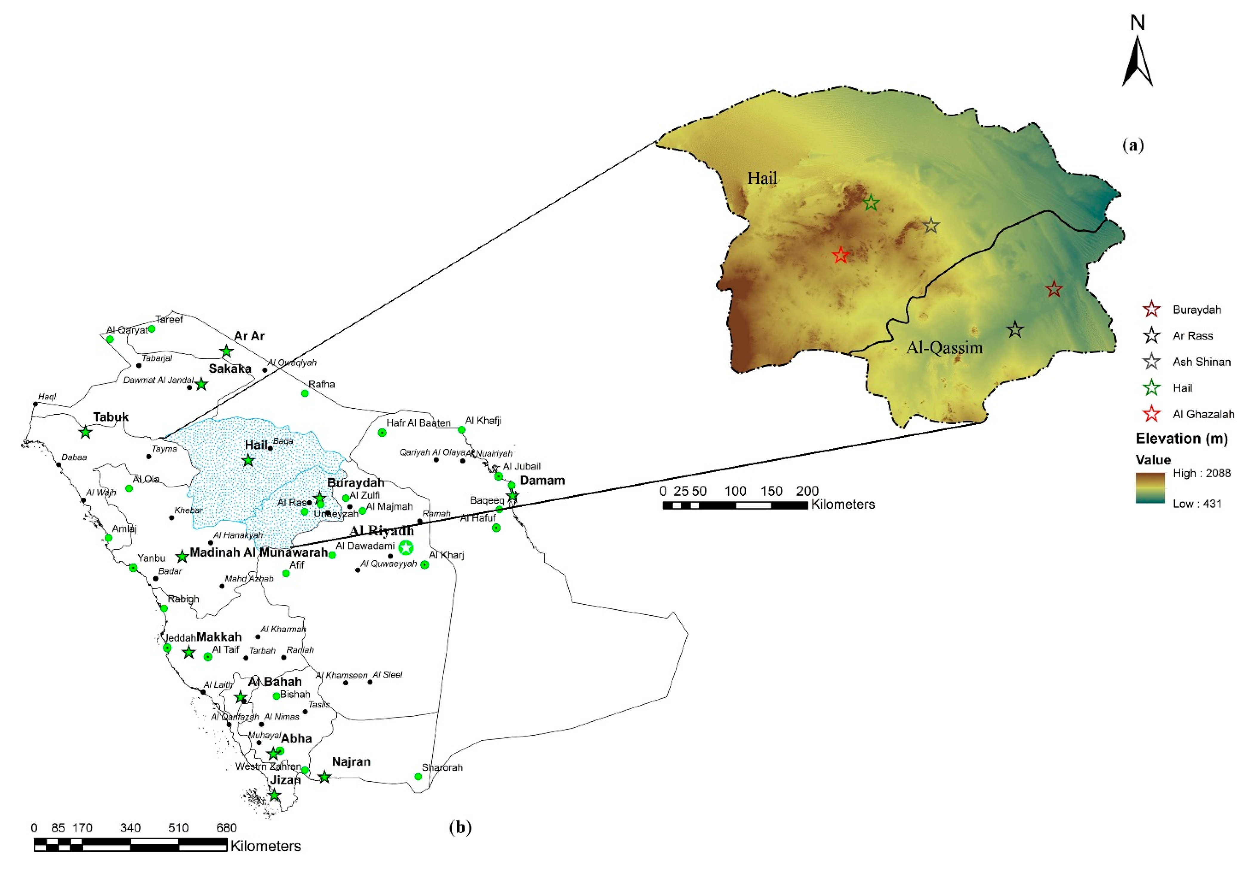
This study was conducted in the Al-Qassim and Hail regions in the central part of the kingdom of Saudi Arabia (KSA). The regions have a total area of 157,000 km2 (Figure 1a). The predominant terrain according to the digital elevation model (DEM) is plain lands with some peaks higher than 2000 m (Figure 1b). Five cities across both regions are selected to perform the study: Buraydah, Ar Rass and Ash Shinan from Al-Qassim and Hail and Al Ghazalah from Hail. Their altitudes vary from 616 to 1083 m above sea level.
2.2. Data Sources and Preparation
The available monthly records of precipitation, maximum and minimum air temperature of the selected locations were obtained from two data sources: the first is the Global Precipitation Climatology Center [34], while the second is the Presidency of Meteorology and Environment (PME) of the KSA. Data from both sources were compared to each other in order to complete the missing data and establish data series for the period 1950–2011. The other missing climatic data were estimated from the neighboring weather stations using linear regression methods [35]. The quality of established data series was investigated through non-parametric tests.
A long-term dataset for SPEI series of 3-, 6-, 12- and 24-month time scales for each selected location (Figure 1b) were created from the Global SPEI database (SPEIbase V2.0) [36]. This database offers long-time, robust information about drought conditions at the global scale, with a 0.5-degree spatial resolution and a monthly time resolution. It has also a multi-scale character that provides time-scales for the SPEI between 1 and 48 months. This dataset is made available under the open database license [37]. According to drought classification based on SPEI (Table 1), drought events occur at a time when the value of SPEI is negative, while they end when the SPEI value turns positive. The calculation of the SPEI in V2.0 is based on the original SPI (the calculation procedure is described in detail by Li et al., [38]) and the climatic water balance (PCPN-PET) that uses the FAO-56 Penman–Monteith equation [39]. The PET equation can be expressed as follows:
where Δ is the slope of the vapor pressure curve (kPa·°C−1), Rn the surface net radiation (MJ·m−2·day−1), G the soil heat flux density (MJ·m−2·day−1), the psychometric constant (kPa·°C−1), T the mean daily air temperature (°C−1), U2 the wind speed (m·s−1), es the saturated vapor pressure and ea the actual vapor pressure.
Figure 1.
(a) Map of the administrative regions of the Kingdom of Saudi Arabia (KSA) with the indication of the study location (dotted blue area). (b) Digital elevation map for Al-Qassim and Hail with the study’s selected weather stations that are used in this paper.
Figure 1.
(a) Map of the administrative regions of the Kingdom of Saudi Arabia (KSA) with the indication of the study location (dotted blue area). (b) Digital elevation map for Al-Qassim and Hail with the study’s selected weather stations that are used in this paper.

Table 1.
Classes of dryness/wetness grade according to the Standardized Precipitation Evapotranspiration (SPEI) values.
| SPEI Value | SPEI Classes |
|---|---|
| SPEI ≤ −2 | Extremely dry |
| −2 < SPEI ≤ −1.5 | Severely dry |
| −1.5 < SPEI ≤ −1 | Moderately dry |
| −1 < SPEI ≤ 1 | Near normal |
| 1 < SPEI ≤ 1.5 | Moderately wet |
| 1.5 < SPEI ≤ 2 | Severely wet |
| SPEI ≥ 2 | Extremely wet |
2.3. Autoregressive Integrated Moving Average (ARIMA) Modelling Approach
Stochastic or time series models (ARIMA) are an approach of time series forecasting. The models provide a systematic-empirical method for forecasting and analyzing the hydrologic time series data. Therefore, the Box-Jenkins approach for ARIMA model development allows an appropriate remedy for non-stationarity in the historical time series data. This property of the ARIMA model is due to the combination of the autoregressive (AR) and moving average (MA) parts. The AR and MA create the multiplicative ARIMA (p, d, q) (P, D, Q)S model, where (p, d, q) is the non-seasonal part and (P, D, Q)S is the seasonal part of the model. The non-seasonal part of the ARIMA model (AR) can be expressed as:
where and are polynomials for p and q order, respectively.
Meanwhile, the seasonal part of the ARIMA model that defines the multiplicative seasonal of model can be written as:
where p, d and q are non-negative integers that refer to the order of the autoregressive, integrated and moving average parts of the model, respectively; and P, D, Q and S are the order of seasonal auto-regression, the number of seasonal differencing, the order of seasonal moving average and the length of the season, respectively. , , , and are coefficients of the polynomials.
2.4. Autoregressive Integrated Moving Average (ARIMA) Model Development
Basically, the development and selection of the appropriate ARIMA model are achieved by an iterative procedure that consists of three steps [27,40,41]; these steps are as follows.
2.4.1. Model Identification
This step consists of identifying the possible ARIMA model that represents the behavior of the time series. The series behavior was investigated by the autocorrelation function (ACF) and partial autocorrelation function (PACF). The ACF and PACF were used to assist in determining the order of the model. The information provided by ACF and PACF is useful to suggest the type of models that can be built. The final model was then selected using the penalty function statistics through the Akaike information criterion (AIC) and Schwarz-Bayesian criterion (SBC). These criteria help to rank models (models having the lowest value of criterion being the best). The AIC and SBC take the mathematical form as shown below:
where k is number of parameters in the model, (p + q + P + Q); L is the likelihood function of the ARIMA model; and n is the number of observations.
2.4.2. Parameter Estimation
After identifying the appropriate model as an essential step, the estimation of model parameters was achieved. The model estimate values for the AR and MA parts were calculated using the procedure suggested by Box and Jenkins [40]. The AR and MA parameters were tested to make sure that they are statistically significant or not. The associated parameters, such as standard error of estimates and their related t-values, are also calculated.
2.4.3. Diagnostic Checking
Diagnosing the ARIMA model is a crucial part and the last step of the model development. It refers to the model adequacy that checks the model assumptions certainly. This model adequacy assures that the time series satisfies the model assumptions and that the forecast is reliable. Several diagnostic statistics and plots of residuals are investigated to see if the residuals are correlated white noise or not. The conducted residuals analysis of each SPEI fitted model is summarized as follows: ACF and PACF of residuals, histograms of residuals and residual distribution around the mean. The performance of the predictions resulting from the ARIMA (p, d, q) (P, D, Q)S models was evaluated by the following measures for goodness-of-fit:
where N is the number of forecasting events, Xm the observed SPEI and Xs the predicted SPEI.
In this study, all of the SPEI forecasting ARMIA models have been developed using the forecasting feature incorporated in the IBM SPSS 20 software [42]. Since the seasonal models require a periodicity, the seasonal cycle was set as an integer equal to 12.
3. Results and Discussion
3.1. Climate Descriptive Analysis
A descriptive analysis of climatic parameters was conducted as an attempt to understand the behavior of drought over the study area better. Table 2 represents annual means of the most drought-relevant parameters. Based on statistical reasoning, there are no significant differences in mean annual temperatures between the studied meteorological stations; where the highest temperature value was recorded in Ar Rass City (26.44 °C·year−1). Meanwhile, the lowest value was recorded in Hail City (21.83 °C·year−1). Concurrently, the monthly maximum mean temperature occurred in June, July and August; whereas the lowest monthly mean temperature was recorded in December, January and February. Generally, Al-Qassim is warmer than Hail; this slight rise in monthly mean temperature may be due to the variation in altitudes in both regions.
Along with the temperature, the monthly mean precipitation is varied over the year. Generally, very low precipitation rates are in most months of the year, except June, July, August and September having without no precipitation. Both regions presently have a high difference between the monthly mean precipitation and PET (water deficit), as presented in Table 2. The water deficit for Buraydah, Ar Rass, Ash Shinan, Hail and Al Ghazalah were 165.37, 169.12, 146.46, 131.74 and 162.4 mm year−1, respectively. This deficit in water supply needs to be compensated by other water resources and/or following good water management and rationalization methods. Similar trends of PET appear in many places in the world, such as China [43].
Overall, the analysis of drought-relevant climatic parameters for both regions is proving notable decreasing levels in precipitation. This precipitation associates with a significant increase in temperature. Therefore, this situation will drive an acute increment in the frequency and magnitude of drought episodes [44,45]. In fact, the primary reason for concern about turning to drought conditions is that they have a direct negative impact on the actual water resources.
Table 2.
Coordinates and altitude of the weather stations used in this study with drought-relevant climatic parameters.
| No. | Station | Altitude (a.m.s.l) | Time Series | Latitude | Longitude | Tm, °C·year−1 | Pm, mm·year−1 | PET, mm year−1 |
|---|---|---|---|---|---|---|---|---|
| 1 | Buraydah | 616 | 1950−2011 | 26ᵒ21′51.89″ | 43ᵒ58′18.93″ | 24.28 | 19.92 | 185.29 |
| 2 | Ar Rass | 692 | 1950−2011 | 25ᵒ51′46.39″ | 43ᵒ29′11.91″ | 26.44 | 15.21 | 184.33 |
| 3 | Ash Shinan | 914 | 1950−2011 | 27ᵒ09′27.79″ | 42ᵒ26′22.48″ | 22.96 | 18.25 | 161.71 |
| 4 | Hail | 1005 | 1950−2011 | 27ᵒ26′20.44″ | 41ᵒ41′28.59″ | 21.83 | 20.36 | 152.10 |
| 5 | Al Ghazalah | 1083 | 1950−2011 | 26ᵒ47′14.72″ | 41ᵒ18′53.97″ | 25.87 | 13.15 | 175.55 |
Tm = mean annual temperature; Pm = mean annual precipitation; PET = potential evapotranspiration.
3.2. Drought Frequency Variations
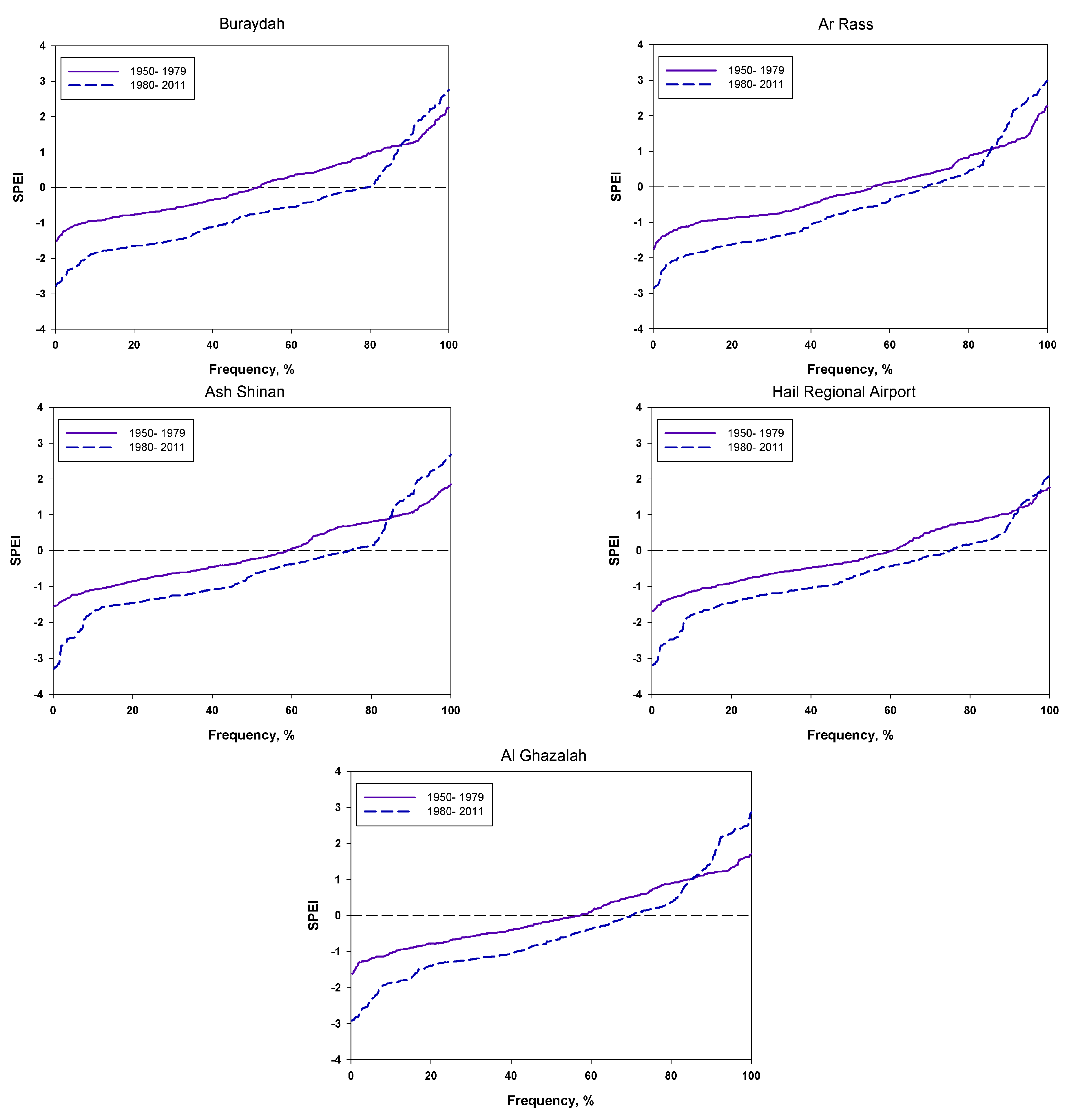
The SPEI time series plots at different time scales covering the period 1950–2011 for Al-Qassim and Hail regions are depicted in Figure 2. These figures show that the whole study area is going toward more droughts. For a deeper investigation of drought variation frequency, the time series of the study period is divided into two main sub-periods (i.e., 1950–1979 and 1981–2011) for both regions. The drought frequencies are calculated and then plotted in Figure 3. Generally, the frequency curve of the first sub-period was almost above the curve of the second period; therefore, an increasing drought frequency was occurring during both sub-periods in all areas. In the first sub-period (1950–1979), a moderately dry condition was relatively low in comparison with the second sub-period (1981–2011). The drought frequency was 0.58%, 1.39%, 2.21%, 2.67 and 0.80% in Buraydah, Ar Rass, Ash Shinan, Hail and Ghazalah, respectively. Meanwhile, there is a significant increase in the drought frequencies (moderately dry condition) during the second sub-period. These frequencies are 19.90%, 17.52%, 20.38%, 15.73% and 17.21% in Buraydah, Ar Rass, Ash Shinan, Hail and Ghazalah, respectively. Based on this analysis, the drought episodes become more frequent in all study areas.
Figure 4 depicts the SPEI at different time scales for Buraydah and Hail cities during the study period. As is evident from this figure, the drought episodes are fluctuating in both cities. In the first five decades, the overall drought trend is approaching the natural limits of near normal and moderately wet scales with intermittent anomalous values in some years. These anomalous values are attributed to rainfall scarcity; whereas, in the last decade, the onset of drought conditions with severely and extremely dry began to emerge. Both cities represent a similar time evolution, with minimal distinguished differences between them. This circumstance is a result of climate change impact [8] and appears in other places in the world, e.g., Egypt [22], Turkey [46], Portugal [47] and China [24].
Figure 2.
Standardized Precipitation Evapotranspiration Index (SPEI) series at different time scales for Al-Qassim and Hail regions during 1950–2011.
Figure 2.
Standardized Precipitation Evapotranspiration Index (SPEI) series at different time scales for Al-Qassim and Hail regions during 1950–2011.
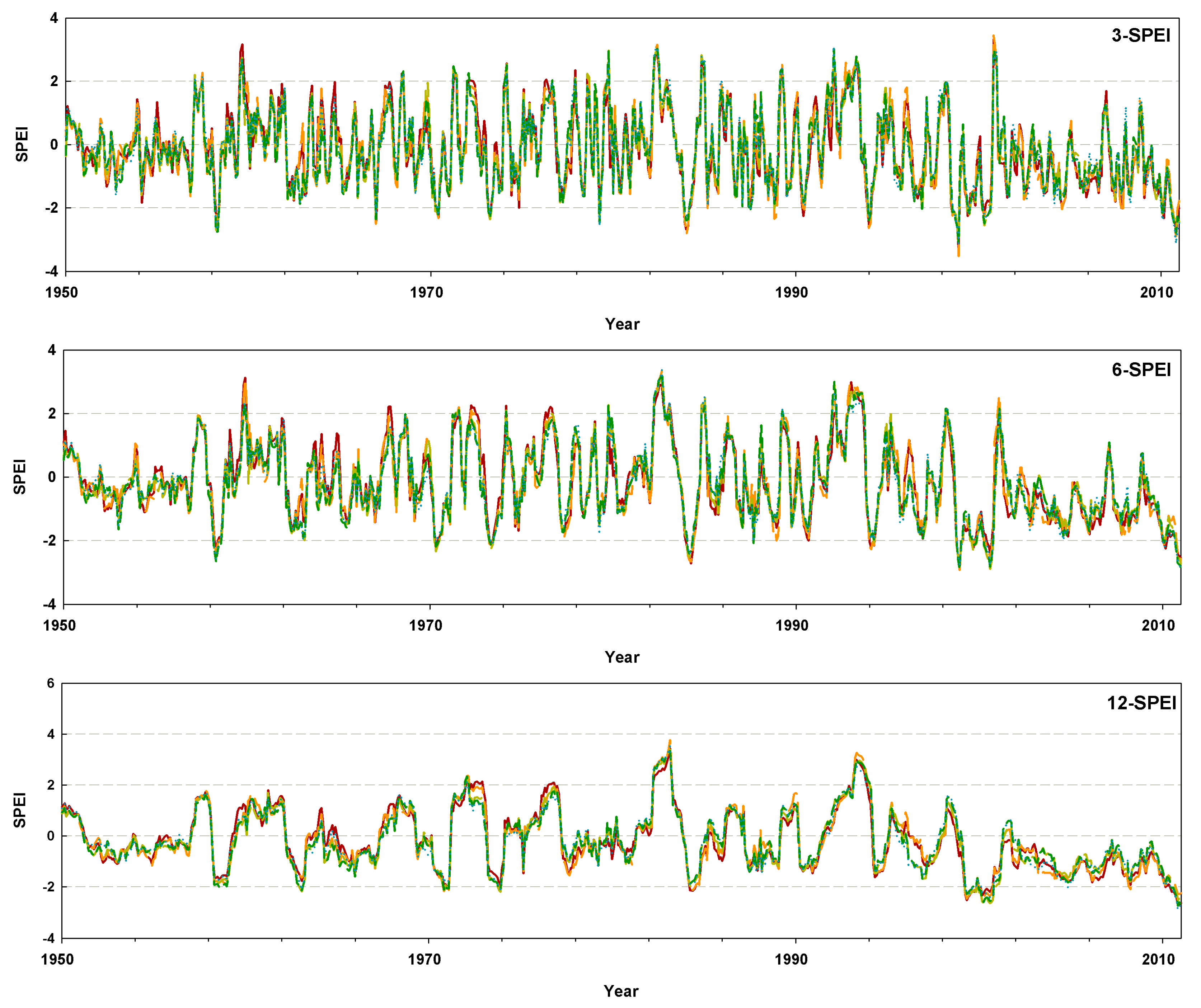

Figure 3.
Drought cumulative percent of the Standardized Precipitation Evapotranspiration Index (SPEI) series over a 24-month time scale for different locations within the central area of Saudi Arabia.
Figure 3.
Drought cumulative percent of the Standardized Precipitation Evapotranspiration Index (SPEI) series over a 24-month time scale for different locations within the central area of Saudi Arabia.

Figure 4.
Temporal evolution for the data series of Standardized Precipitation Evapotranspiration Index (SPEI) at time scales from one to 24 months for the period 1950–2010 in (a) Buraydah and (b) Hail cities.
Figure 4.
Temporal evolution for the data series of Standardized Precipitation Evapotranspiration Index (SPEI) at time scales from one to 24 months for the period 1950–2010 in (a) Buraydah and (b) Hail cities.

3.3. Autoregressive Integrated Moving Average (ARIMA) Model Development
Although it is difficult to forecast drought, relatively reliable drought forecasting remains a vital tool for water resource managers. Thus, in this study, a number of ARIMA models were developed using the SPEI data series at different time scales. The datasets from 1950 to 1989 were used for model development at 3-, 6-, 12- and 24-SPEI time scale. The ARIMA model development is described briefly for Al Ghazalah City as an instance.
3.3.1. Model Identification
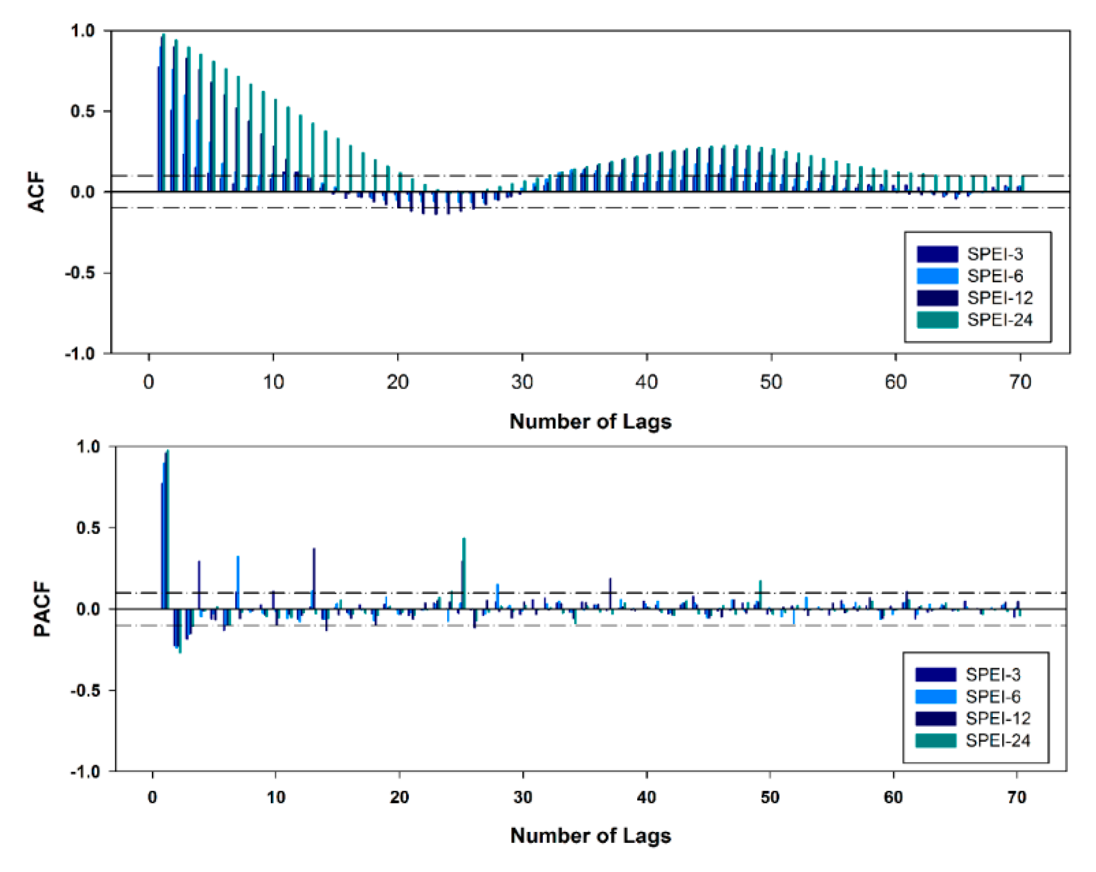
Looking at the sample ACF and PACF plots of the time series in Figure 5, there are non-seasonal and seasonal pattern in the time series. The ACF is damping out in a sine-wave behavior with some significant spikes along the time series. There is a significant spike at Lag 1 in the PACF, which refers to AR (1) as the non-seasonal part of the ARIMA model. The final model selection was based on the lowest values of the penalty function statistics (AIC and SBC). The identified best models for all cities at different SPEI time scales according to minimum AIC and SBC are shown in Table 3.
Table 3.
Autoregressive integrated moving average (ARIMA) models of Standardized Precipitation Evapotranspiration Index for various study areas with forecasting fit measures and penalty function statistics for each estimated model of observed and predicted data.
| Area | SPEI Time Series | ARIMA Model | Fit Measures | Penalty Function Statistics | |||
|---|---|---|---|---|---|---|---|
| R2 | RMSE | MAE | AIC | SBC | |||
| Buraydah | 3 | (1, 0, 2) (0, 0, 0) | 0.670 | 0.698 | 0.542 | 239.254 | 253.091 |
| 6 | (0, 0, 5) (1, 0, 1) | 0.831 | 0.498 | 0.373 | 467.596 | 499.880 | |
| 12 | (0, 1, 2) (0, 0, 1) | 0.944 | 0.281 | 0.189 | 826.347 | 840.180 | |
| 24 | (1, 1, 0) (2, 0, 1) | 0.972 | 0.192 | 0.128 | 1076.379 | 1094.821 | |
| Ar Rass | 3 | (0, 0, 3) (0, 0, 0) | 0.647 | 0.730 | 0.566 | 210.688 | 224.525 |
| 6 | (1, 0, 6) (0, 0, 0) | 0.812 | 0.533 | 0.377 | 423.325 | 455.609 | |
| 12 | (0, 1, 1) (0, 0, 1) | 0.931 | 0.318 | 0.204 | 743.279 | 752.500 | |
| 24 | (1, 1, 0) (2, 0, 1) | 0.966 | 0.218 | 0.138 | 993.164 | 1011.607 | |
| Ash Shinan | 3 | (1, 0, 3) (0, 0, 0) | 0.659 | 0.706 | 0.531 | 235.168 | 253.616 |
| 6 | (0, 0, 5) (0, 0, 0) | 0.830 | 0.494 | 0.363 | 468.527 | 491.588 | |
| 12 | (0, 1, 1) (0, 0, 1) | 0.942 | 0.282 | 0.190 | 821.192 | 830.413 | |
| 24 | (1, 1, 0) (2, 0, 1) | 0.970 | 0.93 | 0.129 | 1071.550 | 1089.993 | |
| Hail | 3 | (1, 0, 3) (0, 0, 0) | 0.656 | 0.708 | 0.534 | 232.990 | 251.438 |
| 6 | (0, 0, 5) (0, 0, 0) | 0.830 | 0.492 | 0.363 | 470.854 | 493.915 | |
| 12 | (0, 1, 1) (0, 0, 1) | 0.942 | 0.281 | 0.190 | 824.935 | 834.157 | |
| 24 | (1, 1, 0) (2, 0, 1) | 0.970 | 0.194 | 0.130 | 1067.399 | 1,085.842 | |
| Al Ghazalah | 3 | (1, 0, 3) (0, 0, 0) | 0.677 | 0.677 | 0.511 | 261.893 | 280.342 |
| 6 | (1, 0, 5) (0, 0, 0) | 0.845 | 0.464 | 0.337 | 511.111 | 538.783 | |
| 12 | (0, 1, 2) (0, 0, 1) | 0.948 | 0.263 | 0.179 | 868.984 | 882.816 | |
| 24 | (1, 1, 0) (2, 0, 1) | 0.974 | 0.180 | 0.121 | 1117.324 | 1135.766 | |
R2 = coefficient of determination; RMSE = root mean square error; MAE = mean absolute error; AIC = Akaike information criterion; SBC = Schwarz-Bayesian criterion.
Figure 5.
Autocorrelation function (ACF) and partial autocorrelation function (PACF) based on a periodicity of 12 months for model selection at different Standardized Precipitation Evapotranspiration Index (SPEI) time series.
Figure 5.
Autocorrelation function (ACF) and partial autocorrelation function (PACF) based on a periodicity of 12 months for model selection at different Standardized Precipitation Evapotranspiration Index (SPEI) time series.

3.3.2. Model Parameter Estimate
Table 4 presents model parameters at different lags, standard error, t-value and the associated significance value at a significance level < 0.05 for Al Ghazalah city. It can be observed that the standard error of most model parameters is very small compared to the parameter values. This is with the exception of the model parameter values of the SPEI at three-month time scale. Additionally, all of the ARIMA model parameters are significant at significance level < 0.05. Thus, these parameters should be combined in the model. The same conclusion was found in the other models.
Table 4.
Statistical analysis of autoregressive integrated moving average (ARIMA) model parameters, including the autoregressive (AR) and moving average (MA) orders with associated significance values at significance level < 0.05 for Al Ghazalah City.
| SPEI Time Series | Parameter | Lag | Estimate Value | Standard Error | t-value | Sig. |
|---|---|---|---|---|---|---|
| 3 | AR | 1 | 0.612 | 0.105 | 5.84 | 0.000 |
| MA | 1 | −0.383 | 0.117 | −3.27 | 0.001 | |
| 2 | −0.361 | 0.104 | −3.46 | 0.001 | ||
| 3 | 0.227 | 0.094 | 2.43 | 0.016 | ||
| 6 | AR | 1 | 0.410 | 0.054 | 7.54 | 0.000 |
| MA | 1 | −0.738 | 0.048 | −15.49 | 0.000 | |
| 2 | −0.647 | 0.054 | −12.01 | 0.000 | ||
| 3 | −0.522 | 0.052 | −9.99 | 0.000 | ||
| 4 | −0.481 | 0.043 | −11.30 | 0.000 | ||
| 5 | −0.545 | 0.033 | −16.74 | 0.000 | ||
| 12 | MA | 1 | −0.223 | 0.037 | −6.08 | 0.000 |
| 2 | −0.088 | 0.037 | −2.41 | 0.016 | ||
| MA, Seasonal | 1 | 0.717 | 0.027 | 26.35 | 0.000 | |
| 24 | AR | 1 | 0.249 | 0.036 | 6.98 | 0.000 |
| AR, Seasonal | 1 | −0.357 | 0.048 | −7.47 | 0.000 | |
| 2 | −0.496 | 0.034 | −14.54 | 0.000 | ||
| MA, Seasonal | 1 | −0.526 | 0.052 | −10.14 | 0.000 |
Sig. = significance value.
3.3.3. Diagnostic Checking of Residuals
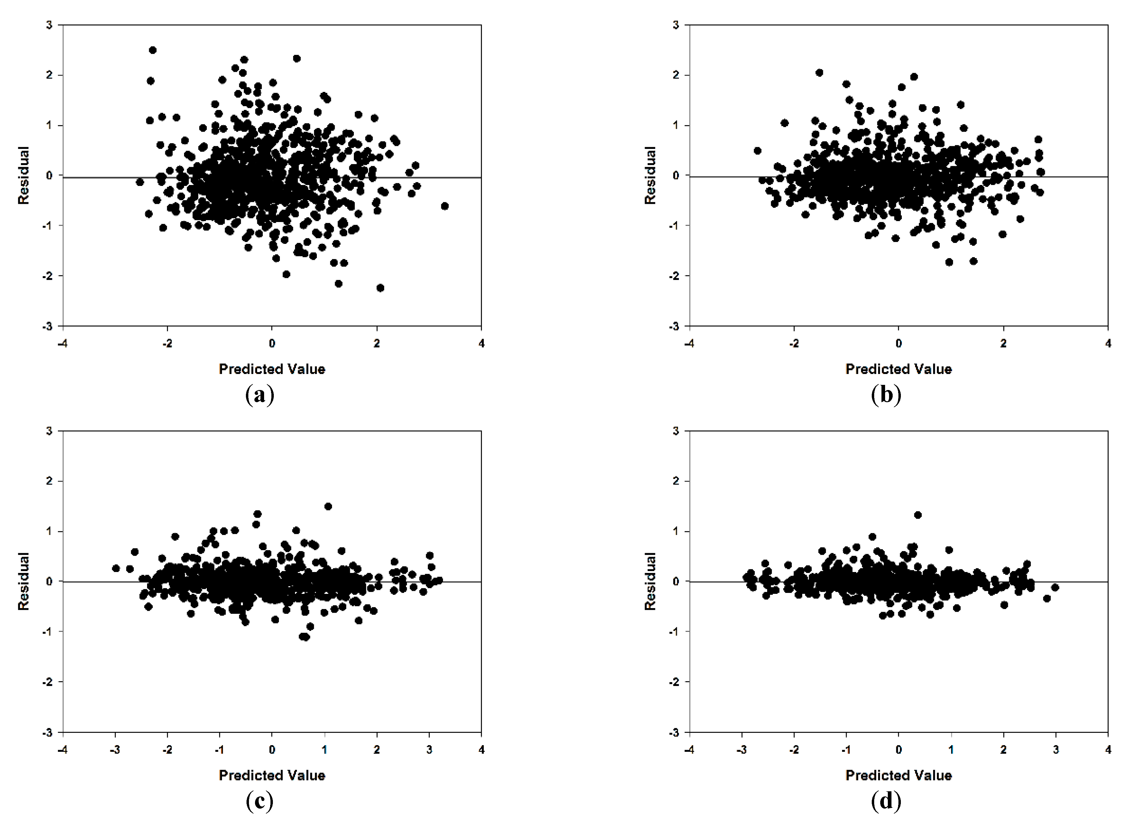
After the estimation of model parameters, diagnostic checking was performed to verify the adequacy of the model. The ACF and PACF of the residuals at different time scales are shown in Figure 6 and Figure 7. All of the ACF and PACF values are within the confidence of 0.01 bands for all lags. Therefore, there is no significant correlation between residuals. Figure 8 depicts the histograms of residuals for the SPEI at different time scales, which are normally distributed. This indicates that the fitted model is adequate for the SPEI time series data and residuals to white noise. Figure 9 shows the scatterplots of the residuals against predicted values of SPEI at different time scales. In this case, the scatterplots show no obvious patterns, and all of the residuals are distributed randomly around zero. Consequently, forecasts of these models are good and adequate.
Table 3 presents the highest accuracy forecasting models related to each considered SPEI time scale with accuracy fit measures (R2, RMSE, and MAE). Generally, drought forecasting with ARIMA models in Al-Qassim and Hail has shown considerable results, with R2 ranging between 0.656 and 0.974. However, in most cases, the R2 of all ARIMA models increases to greater than 0.8, which matches with the lower values of RMSE and MAE. This is with the exception of ARIMA models at the three-month time scales, which demonstrate the lowest R2 values. Therefore, it can be summarized that the ARIMA models with longer time scales are manifesting a forecasting ability and fitting accurately with the drought prediction in the future. Very similar results appear around the world and apply to the SPI, which is the basis of the SPEI, i.e., China [48] and India [29].
It is noted that the SPEI time series for all cities has almost the same trend for similar time series (Figure 2). Additionally, the signals of the 12-SPEI and 24-SPEI time series are similar; similarly for the signals of the 3-SPEI and 6-SPE time series. Therefore, the order d equal to one appears for the time series based on 12 and 24 months, while this do not appear in the corresponding 3- and 6-month scales.
Figure 6.
Autocorrelation function (ACF) of residuals of Al Ghazalah City as a best-fitted model for data series of standardized precipitation evapotranspiration index (SPEI) at different time scales during the period of 1950–2010; (a) 3-SPEI, (b) 6-SPEI, (c) 12-SPEI and (d) 24-SPEI.
Figure 6.
Autocorrelation function (ACF) of residuals of Al Ghazalah City as a best-fitted model for data series of standardized precipitation evapotranspiration index (SPEI) at different time scales during the period of 1950–2010; (a) 3-SPEI, (b) 6-SPEI, (c) 12-SPEI and (d) 24-SPEI.
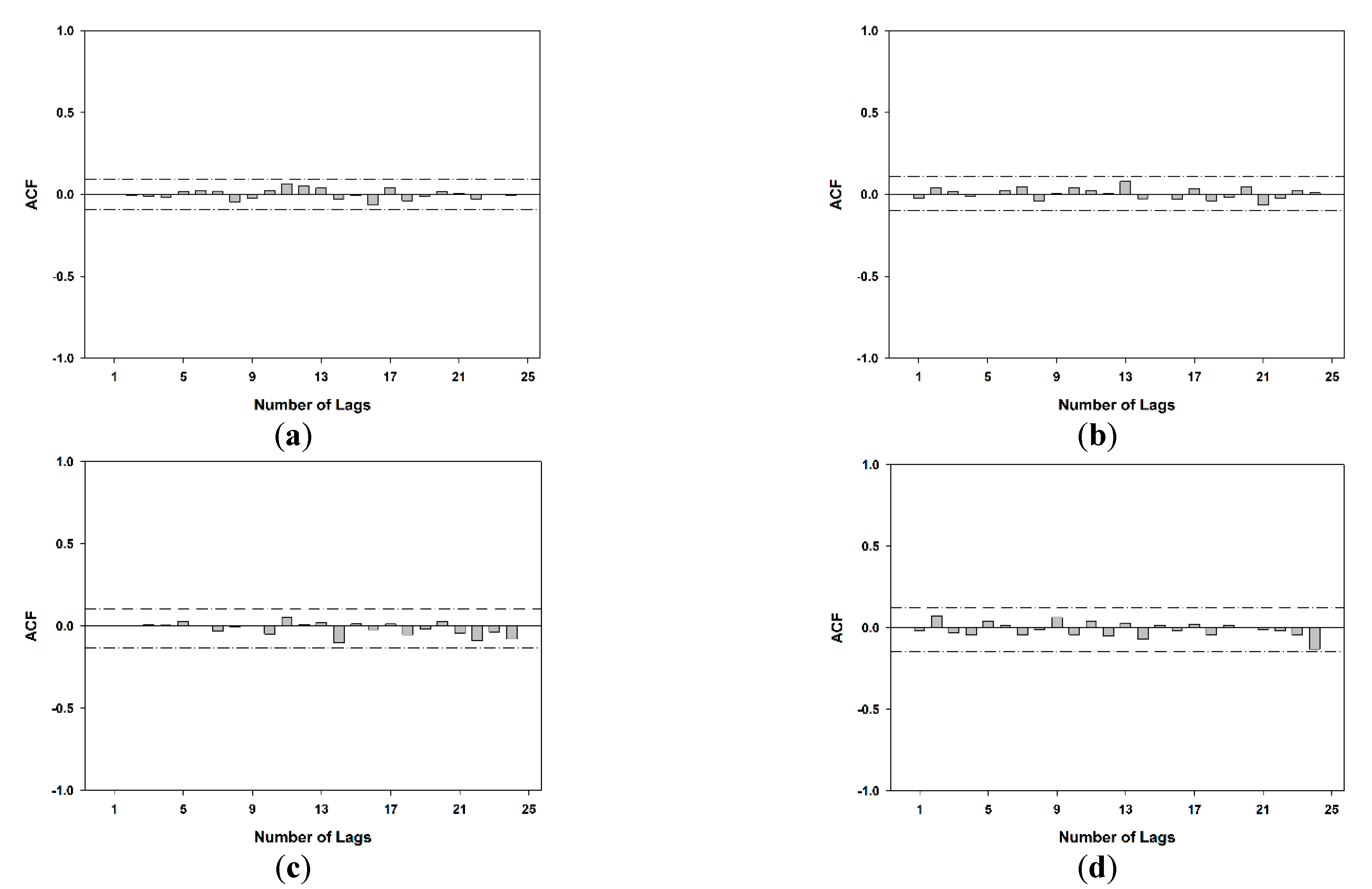
Figure 7.
Partial autocorrelation function (PACF) of residuals of Al Ghazalah City as a best-fitted model for data series of standardized precipitation evapotranspiration index (SPEI) at different time scales during the period of 1950–2010: (a) 3-SPEI, (b) 6-SPEI, (c) 12-SPEI and (d) 24-SPEI.
Figure 7.
Partial autocorrelation function (PACF) of residuals of Al Ghazalah City as a best-fitted model for data series of standardized precipitation evapotranspiration index (SPEI) at different time scales during the period of 1950–2010: (a) 3-SPEI, (b) 6-SPEI, (c) 12-SPEI and (d) 24-SPEI.
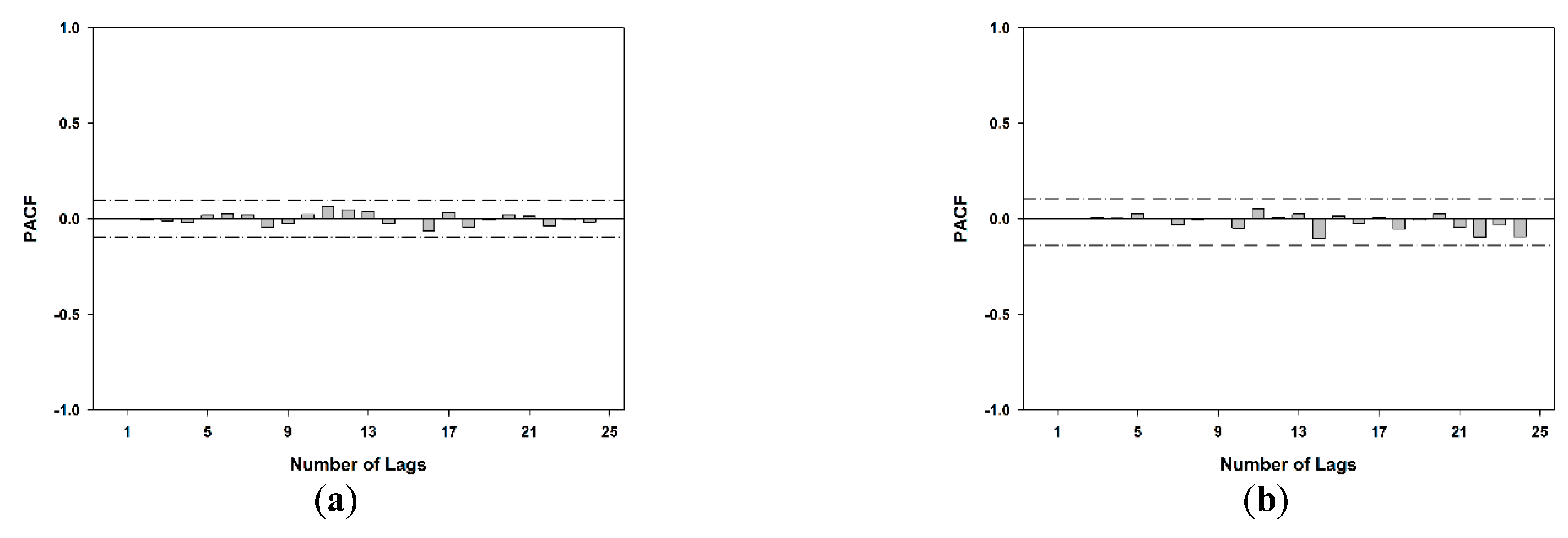

Figure 8.
Histogram of residuals of Al Ghazalah City as a best-fitted model for data series of standardized precipitation evapotranspiration index SPEI at different time scales during the period of 1950–2010: (a) 3-SPEI, (b) 6-SPEI, (c) 12-SPEI and (d) 24-SPEI.
Figure 8.
Histogram of residuals of Al Ghazalah City as a best-fitted model for data series of standardized precipitation evapotranspiration index SPEI at different time scales during the period of 1950–2010: (a) 3-SPEI, (b) 6-SPEI, (c) 12-SPEI and (d) 24-SPEI.

Figure 9.
Residuals vs. predicted values of Al Ghazalah City as a best-fitted model for data series of standardized precipitation evapotranspiration index (SPEI) at different time scales during the period of 1950–2010: (a) 3-SPEI, (b) 6-SPEI, (c) 12-SPEI and (d) 24-SPEI.
Figure 9.
Residuals vs. predicted values of Al Ghazalah City as a best-fitted model for data series of standardized precipitation evapotranspiration index (SPEI) at different time scales during the period of 1950–2010: (a) 3-SPEI, (b) 6-SPEI, (c) 12-SPEI and (d) 24-SPEI.

3.3.4. Model Forecasting
Obviously, forecasting plays an important role in decision making. It can help to foresee the future uncertainty based on the behavior of the past and current observations. The forecasting through the ARIMA models provides a good basis for hydrologic phenomena. For drought forecasting, one city from each region has been selected and then used to forecast drought. The testing data series of the SPEI at different time scales is from 1990 to 2011. The predicted and observed SPEI were plotted for evaluating the extent of agreement between both data series; Buraydah and Hail cities represent Al-Qassim and Hail regions, respectively. The comparison of both observed and predicted data (Figure 10 and Figure 11) illustrates the high accuracy of forecasted values. Undoubtedly, by increasing the number of SPEI time series, the ability of the model to forecast the future will be enhanced. The reason for the enhancement is that the increasing number of SPEI time series refines the SPEI’s output values, which decreases abrupt shifts of the SPEI curve.
By comparing the AR and MA coefficients, it is found that the ARIMA models of the 24-month time scale for Buraydah and Ar Rass are quite similar. Meanwhile, the ARIMA models of three-month time scale are similar in Ash Shinan, Hail and Al Ghazalah. The same remarks were realized with ARIMA models of the 24-month time scale. Table 5 presents the similar parameter estimates between the developed ARIMA models for both regions. From the results in Table 3, the values of p, d, q, P, D and Q obtained from the models fitted for the five cities are quite similar at the same time scales. Therefore, the ARIMA model (1, 1, 0) (2, 0, 1) at 24-SPEI could be generalized for the entire Al-Qassim region. Additionally, the ARIMA model (1, 0, 3) (0, 0, 0) at 3-SPEI and the ARIMA model (1, 1, 1) (2, 0, 1) at 24-SPEI could be applied to the whole Hail region. This is because they are located near each other.
Table 5.
Similar parameter estimate values at the same Standardized Precipitation Evapotranspiration Index (SPEI) time scale including the autoregressive (AR) and moving average (MA) orders with associated significance values at significance level < 0.05 for both regions.
| Region | City | SPEI Time Series | Parameter | Lag | Estimate Value | SE | t-value | Sig. |
|---|---|---|---|---|---|---|---|---|
| Al-Qassim | Buraydah | 24 | AR | 1 | 0.204 | 0.036 | 5.64 | 0.000 |
| -- | AR, Seasonal | 1 | −0.186 | 0.051 | −3.63 | 0.000 | ||
| -- | -- | 2 | −0.536 | 0.032 | −16.77 | 0.000 | ||
| -- | MA, Seasonal | 1 | −0.319 | 0.061 | −5.27 | 0.000 | ||
| Ar Rass | 24 | AR | 1 | 0.172 | 0.036 | 4.73 | 0.000 | |
| -- | AR, Seasonal | 1 | −0.247 | 0.050 | −4.90 | 0.000 | ||
| -- | -- | 2 | −0.525 | 0.033 | −16.14 | 0.000 | ||
| -- | MA, Seasonal | 1 | −0.386 | 0.058 | −6.62 | 0.000 | ||
| Hail | Ash Shinan | 3 | AR | 1 | 0.609 | 0.116 | 5.24 | 0.000 |
| -- | MA | 1 | −0.373 | 0.128 | −2.91 | 0.004 | ||
| -- | -- | 2 | −0.328 | 0.115 | −2.85 | 0.004 | ||
| -- | -- | 3 | 0.239 | 0.100 | 2.38 | 0.017 | ||
| 24 | AR | 1 | 0.223 | 0.036 | 6.21 | 0.000 | ||
| -- | AR, Seasonal | 1 | −0.304 | 0.050 | −6.08 | 0.000 | ||
| -- | -- | 2 | −0.495 | 0.034 | −14.60 | 0.000 | ||
| -- | MA, Seasonal | 1 | −0.474 | 0.055 | −8.57 | 0.000 | ||
| Hail | 3 | AR | 1 | 0.636 | 0.113 | 5.61 | 0.000 | |
| -- | MA | 1 | −0.343 | 0.126 | −2.73 | 0.007 | ||
| -- | -- | 2 | −0.286 | 0.114 | −2.51 | 0.012 | ||
| -- | -- | 3 | 0.260 | 0.098 | 2.66 | 0.008 | ||
| 24 | AR | 1 | 0.232 | 0.036 | 6.47 | 0.000 | ||
| -- | AR, Seasonal | 1 | −0.358 | 0.049 | −7.28 | 0.000 | ||
| -- | -- | 2 | −0.473 | 0.035 | −13.63 | 0.000 | ||
| -- | MA, Seasonal | 1 | −0.537 | 0.053 | −10.22 | 0.000 | ||
| Al Ghazalah | 3 | AR | 1 | 0.612 | 0.105 | 5.84 | 0.000 | |
| -- | MA | 1 | −0.383 | 0.117 | −3.27 | 0.001 | ||
| -- | -- | 2 | −0.361 | 0.104 | −3.46 | 0.001 | ||
| -- | -- | 3 | 0.227 | 0.094 | 2.43 | 0.016 | ||
| 24 | AR | 1 | 0.249 | 0.036 | 6.98 | 0.000 | ||
| -- | AR, Seasonal | 1 | −0.357 | 0.048 | −7.47 | 0.000 | ||
| -- | -- | 2 | −0.496 | 0.034 | −14.54 | 0.000 | ||
| -- | MA, Seasonal | 1 | −0.526 | 0.052 | −10.14 | 0.000 |
Sig. = significance value.
Figure 10.
Observed and predicted standardized precipitation evapotranspiration index (SPEI) series over different time scales based on mean precipitation during 1990 to 2011 for Buraydah City.
Figure 10.
Observed and predicted standardized precipitation evapotranspiration index (SPEI) series over different time scales based on mean precipitation during 1990 to 2011 for Buraydah City.
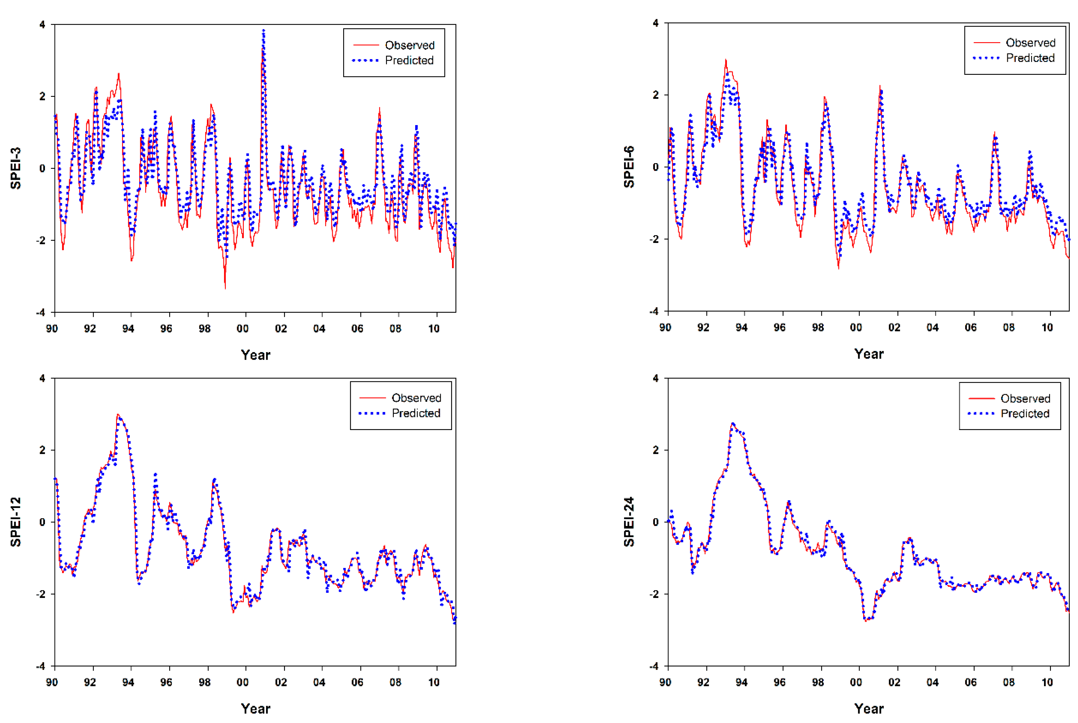
Figure 11.
Observed and predicted standardized precipitation evapotranspiration index (SPEI) series over different time scales based on mean precipitation during 1990 to 2011 for Hail City.
Figure 11.
Observed and predicted standardized precipitation evapotranspiration index (SPEI) series over different time scales based on mean precipitation during 1990 to 2011 for Hail City.

4. Conclusions
In this work, the SPEI is presented as a powerful multi-scalar drought index to investigate drought event variations in Al-Qassim and Hail regions. The objective of this study has been divided into two parts. The first part of the objective is the assessment of climatic parameters and drought frequency based on SPEI. According to this assessment, both regions are suffering from the presence of water deficit condition up to 169.12 mm·year−1 in Ar Rass City as a result of high temperatures that are associated with low precipitation rates. Therefore, the risk of drought occurrence increases due to the water deficit, which eventually will create tremendous threats to water resources. At the same time, the SPEI variation is going towards an abnormal trend of drought (severely and extremely dry) since the last decade. Anyway, these results should sound alarm bells in hyper-arid regions.
It is worth noting that one of the most problematic issues facing hydrologists is forecasting drought events. Hence, the second part of the objective was developing and testing the ARMIA models for drought forecasting using SPEI with 3-, 6-, 12-, 24-month time scales. Based on the AIC and SBC values, the best ARIMA models were identified. The reliability of forecasted future values is a core point for forecasters. This is because the drought mitigation policies will be implemented based on the forecasted values. Thus, after the estimation of the parameters of selected models, a series of diagnostic checking tests were performed. Among the possible ARIMA models, the ARIMA model (1, 1, 0) (2, 0, 1) at 24-SPEI could be chosen as a general model for the Al-Qassim region. Meanwhile, the ARIMA model (1, 0, 3) (0, 0, 0) at 3-SPEI and the ARIMA model (1, 1, 1) (2, 0, 1) at 24-SPEI could be generalized for the Hail region. These results may be due to the cities being located near each other. It is also noted that the results obtained from the ARIMA models for the studied cities showed that the ARIMA model at the 24-SPEI time scale is the best forecasting model, which matches the high coefficient of determination R2 (more than 0.9) and lower values of RMSE and MAE. Meanwhile, the ARIMA model at the 3-SPEI time scale is the worst model for drought prediction for all cities. Since these ARIMA models show their powerful ability in drought forecasting, they can play a very important role as useful tools for water resource managers and planners to take precautions considering drought for other hyper-arid regions in advance.
Obviously, the linkage between the climate change represented in droughts and available water resources is necessary. Thus, in hyper-arid regions, confronting the actual/future drought conditions with withdrawal/recharge periods of groundwater is one of the most important investigations and should be considered as a priority in future research.
Acknowledgments
The project was financially supported by King Saud University, Vice Deanship of Research Chairs.
Author Contributions
The authors, Amr Mossad and Abdulrahman Ali Alazba, identified the study framework and contributed extensively throughout the whole work. The authors have shared the manuscript preparation and the models development. In addition, the authors analyzed the data and discussed the results of this manuscript throughout all processes. They all read and approved the final manuscript.
Conflicts of Interest
The authors declare no conflict of interest.
References
- Sivakumar, M.V.K. Interactions between climate and desertification. Agr. Forest Meteorol. 2007, 142, 143–155. [Google Scholar] [CrossRef]
- Le Houérou, H.N. Climate change, drought and desertification. J. Arid Environ. 1996, 34, 133–185. [Google Scholar] [CrossRef]
- Hirabayashi, Y.; Kanae, S.; Emori, S.; Oki, T.; Kimoto, M. Global projections of changing risks of floods and droughts in a changing climate. Hydrol. Sci. J. 2008, 53, 754–772. [Google Scholar] [CrossRef]
- Sheffield, J.; Wood, E.F.; Roderick, M.L. Little change in global drought over the past 60 years. Nat. Clim. Change 2012, 491, 435–438. [Google Scholar]
- Wilhite, D.A.; Rosenberg, N.J.; Glantz, M.H. Improving federal response to drought. J. Clim. Appl. Meteorol. 1986, 25, 332–342. [Google Scholar] [CrossRef]
- Heim, R.R. A review of twentieth-century drought indices used in the united states. B. Am. Meteorol. Soc. 2002, 83, 1149–1165. [Google Scholar] [CrossRef]
- Belal, A.-A.; El-Ramady, H.; Mohamed, E.; Saleh, A. Drought risk assessment using remote sensing and GIS techniques. Arab. J. Geosci. 2014, 7, 35–53. [Google Scholar] [CrossRef]
- Mishra, A.K.; Singh, V.P. A review of drought concepts. J. Hydrol. 2010, 391, 202–216. [Google Scholar] [CrossRef]
- Sheffield, J.; Wood, E.F. Drought: Past Problems and Future Scenarios; Taylor & Francis: Earthscan, UK, 2012. [Google Scholar]
- Palmer, W.C. Meteorological Drought; U.S. Department of Commerce, Weather Bureau: Washington, DC, USA, 1965. [Google Scholar]
- Shafer, B.A.; Dezman, L. Development of a Surface Water Supply Index (SWSI) to assess the severity of drought conditions in snowpack runoff Areas. In Proceedings of the Western Snow Conference, Reno, NV, USA, 19–23 April 1982.
- Palfai, I. Description and forecasting of droughts in hungary. In Proceedings of the 14th Congress on Irrigation and Drainage (ICID), Rio de Janario, Brazil, 30 April–4 May 1990.
- McKee, T.; Doesken, N.; Kleist, J. The relation of drought frequency and duration to time scales. In Propeedings of the 8th Conference on Applied Climatology, Anaheim, CA, USA, 17–22 January 1993.
- Vicente-Serrano, S.M.; Beguería, S.; López-Moreno, J.I. A multiscalar drought index sensitive to global warming: The standardized precipitation evapotranspiration index. J. Clim. 2010, 23, 1696–1718. [Google Scholar] [CrossRef]
- Karavitis, C.A.; Alexandris, S.; Tsesmelis, D.E.; Athanasopoulos, G. Application of the standardized precipitation index (SPI) in Greece. Water 2011, 3, 787–805. [Google Scholar] [CrossRef]
- Hayes, M.; Svoboda, M.; Wall, N.; Widhalm, M. The Lincoln declaration on drought indices: Universal meteorological drought index recommended. B. Am. Meteorol. Soc. 2010, 92, 485–488. [Google Scholar] [CrossRef]
- Huang, R.; Yan, D.; Liu, S. Combined characteristics of drought on multiple time scales in Huang-Huai-Hai River basin. Arab. J. Geosci. 2014, 2014. [Google Scholar] [CrossRef]
- Dalezios, N.R.; Loukas, A.; Vasiliades, L.; Liakopoulos, E. Severity-duration-frequency analysis of droughts and wet periods in Greece. Hydrol. Sci. J. 2000, 45, 751–769. [Google Scholar] [CrossRef]
- Bordi, I.; Frigio, S.; Parenti, P.; Speranza, A.; Sutera, A. The analysis of the standardized precipitation index in the mediterranean area: Large-scale patterns. Ann. Geophys. 2001, 44, 965–978. [Google Scholar]
- Shahabfar, A.; Eitzinger, J. Spatio-temporal analysis of droughts in semi-arid regions by using meteorological drought indices. Atmosphere 2013, 4, 94–112. [Google Scholar] [CrossRef]
- Beguería, S.; Vicente-Serrano, S.M.; Reig, F.; Latorre, B. Standardized Precipitation Evapotranspiration Index (SPEI) revisited: Parameter fitting, evapotranspiration models, tools, datasets and drought monitoring. Int. J. Clim. 2013, 34, 3001–3023. [Google Scholar] [CrossRef]
- Mossad, A.; Mehawed, H.; El-Araby, A. Seasonal drought dynamics in El-Beheira governorate, Egypt. Am. J. Environ. Sci. 2014, 10, 140–147. [Google Scholar] [CrossRef]
- Vicente-Serrano, S.M.; López -Moreno, J.I.; Drumond, A.; Gimeno, L.; Nieto, R.; Moran-Tejeda, E.; Lorenzo-Lacruz, J.; Beguería, S.; Zabalza, J. Effects of warming processes on droughts and water resources in the NW Iberian Peninsula (1930–2006). Clim. Res. 2011, 48, 203–212. [Google Scholar] [CrossRef]
- Yu, M.; Li, Q.; Hayes, M.J.; Svoboda, M.D.; Heim, R.R. Are droughts becoming more frequent or severe in China based on the standardized precipitation evapotranspiration index: 1951–2010? Int. J. Clim. 2014, 34, 545–558. [Google Scholar] [CrossRef]
- Panu, U.S.; Sharma, T.C. Challenges in drought research: Some perspectives and future directions. Hydrol. Sci. J. 2002, 47, S19–S30. [Google Scholar] [CrossRef]
- Mishra, A.K.; Singh, V.P. Drought modeling—A review. J. Hydrol. 2011, 403, 157–175. [Google Scholar] [CrossRef]
- Box, G.E.P.; Jenkins, G.M.; Reinsel, G.C. Time Series Analysis: Forecasting and Control; Wiley: Hoboken, NJ, USA, 2008. [Google Scholar]
- Mishra, A.K.; Desai, V.R. Drought forecasting using feed-forward recursive neural network. Ecol. Mode. 2006, 198, 127–138. [Google Scholar] [CrossRef]
- Mishra, A.K.; Desai, V.R. Drought forecasting using stochastic models. Stoch. Environ. Res. Ris. Assess. 2005, 19, 326–339. [Google Scholar] [CrossRef]
- Mishra, A.K.; Singh, V.P. Simulating hydrological drought properties at different spatial units in the united states based on Wavelet-Bayesian regression approach. Earth Interact. 2012, 16, 1–23. [Google Scholar] [CrossRef]
- Özger, M.; Mishra, A.K.; Singh, V.P. Long lead time drought forecasting using a wavelet and fuzzy logic combination model: A case study in Texas. J. Hydrometeorol. 2011, 13, 284–297. [Google Scholar] [CrossRef]
- Ozger, M.; Mishra, A.K.; Singh, V.P. Estimating palmer drought severity index using a wavelet fuzzy logic model based on meteorological variables. Int. J. Clim. 2011, 31, 2021–2032. [Google Scholar] [CrossRef]
- Mishra, A.; Desai, V.; Singh, V. Drought forecasting using a hybrid stochastic and neural network model. J. Hydrol. Eng. 2007, 12, 626–638. [Google Scholar] [CrossRef]
- GPCC. Global Precipitation Climatology Center. Available online: http//gpcc.Dwd.De (accessed on 11 March 2015).
- Ferrari, G.T.; Ozaki, V. Missing data imputation of climate datasets: Implications to modeling extreme drought events. Rev. Brasil. Meteorologia 2014, 29, 21–28. [Google Scholar] [CrossRef]
- SPEIbaseV2.0. Global SPEI Database. Available online: http://sac.csic.es/spei/ (accessed on 11 March 2015).
- ODbL. Open Database License (odbl) v1.0. Available online: http://opendatacommons.org/ (accessed on 11 March 2015).
- Li, X.; Zhang, Q.; Ye, X. Dry/wet conditions monitoring based on TRMM rainfall data and its reliability validation over Poyang Lake basin, China. Water 2013, 5, 1848–1864. [Google Scholar] [CrossRef]
- Allen, R.G.; Pereira, L.S.; Raes, D.; Smith, M. Crop Evapotranspiration: Guidelines for Computing Crop Water Requirements; Food and Agriculture Organization of the United Nations (FAO): Rome, Italy, 1998. [Google Scholar]
- Box, G.E.P.; Jenkins, G.M. Time Series Analysis: Forecasting and Control; Holden-Day: Ann Arbor, MI, USA, 1976. [Google Scholar]
- Brockwell, P.J.; Davis, R.A. Introduction to Time Series and Forecasting; Springer New York: New York, NY, USA, 2013. [Google Scholar]
- SPSS20. IBM Software, SPSS. Available online: http://www-01.Ibm.Com/software/analytics/spss/ (accessed on 11 March 2015).
- Yao, Y.; Zhao, S.; Zhang, Y.; Jia, K.; Liu, M. Spatial and decadal variations in potential evapotranspiration of China based on reanalysis datasets during 1982–2010. Atmosphere 2014, 5, 737–754. [Google Scholar] [CrossRef]
- Blenkinsop, S.; Fowler, H. Changes in European drought characteristics projected by the prudence regional climate models. Int. J. Clim. 2007, 27, 1595–1610. [Google Scholar] [CrossRef]
- Weiß, M.; Flörke, M.; Menzel, L.; Alcamo, J. Model-based scenarios of Mediterranean droughts. Adv. Geosci. 2007, 12, 145–151. [Google Scholar] [CrossRef]
- Sönmez, F.K.; Kömüscü, A.; Erkan, A.; Turgu, E. An analysis of spatial and temporal dimension of drought vulnerability in turkey using the standardized precipitation index. Nat. Hazards 2005, 35, 243–264. [Google Scholar] [CrossRef]
- Paulo, A.A.; Rosa, R.D.; Pereira, L.S. Climate trends and behaviour of drought indices based on precipitation and evapotranspiration in Portugal. Nat. Hazards Earth Syst. Sci. 2012, 12, 1481–1491. [Google Scholar] [CrossRef]
- Han, P.; Wang, P.; Tian, M.; Zhang, S.; Liu, J.; Zhu, D. Application of the ARIMA models in drought forecasting using the standardized precipitation index. In Computer and Computing Technologies in Agriculture VI; Li, D., Chen, Y., Eds.; Springer Berlin Heidelberg: Berlin, Germany, 2013; Volume 392, pp. 352–358. [Google Scholar]
© 2015 by the authors; licensee MDPI, Basel, Switzerland. This article is an open access article distributed under the terms and conditions of the Creative Commons Attribution license (http://creativecommons.org/licenses/by/4.0/).
Share and Cite
MDPI and ACS Style
Mossad, A.; Alazba, A.A. Drought Forecasting Using Stochastic Models in a Hyper-Arid Climate. Atmosphere 2015, 6, 410-430. https://doi.org/10.3390/atmos6040410
AMA Style
Mossad A, Alazba AA. Drought Forecasting Using Stochastic Models in a Hyper-Arid Climate. Atmosphere. 2015; 6(4):410-430. https://doi.org/10.3390/atmos6040410
Chicago/Turabian StyleMossad, Amr, and Abdulrahman Ali Alazba. 2015. "Drought Forecasting Using Stochastic Models in a Hyper-Arid Climate" Atmosphere 6, no. 4: 410-430. https://doi.org/10.3390/atmos6040410