A Methodology to Infer Crop Yield Response to Climate Variability and Change Using Long-Term Observations

Abstract
:1. Introduction
- i.
- Carefully analyse available long-term observations of crop yields in order to infer the most likely crop yield response to climate variability and change;
- ii.
- Use the inferred response to test and calibrate crop models under current conditions.
2. Method
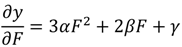
2.1. Approach and Formulations

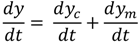
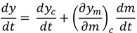
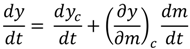
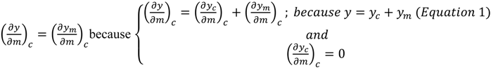
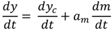
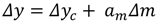
 ) is the crop yield variation as a function of crop management. Δm, Δy and Δyc are the annual variation of crop management, total crop yield and climate-induced crop yield first-differences, respectively.
- i.
- To use crop yield and management observations over the selected sub-period to derive a relationship that statistically links interannual crop yield and crop management variations; and
- ii.
- To apply the obtained relationship between crop yield and management to the entire period of study (i.e., 1961–2006), since that relationship satisfies the climate constant conditions and is time independent.

2.2. Data

3. Results
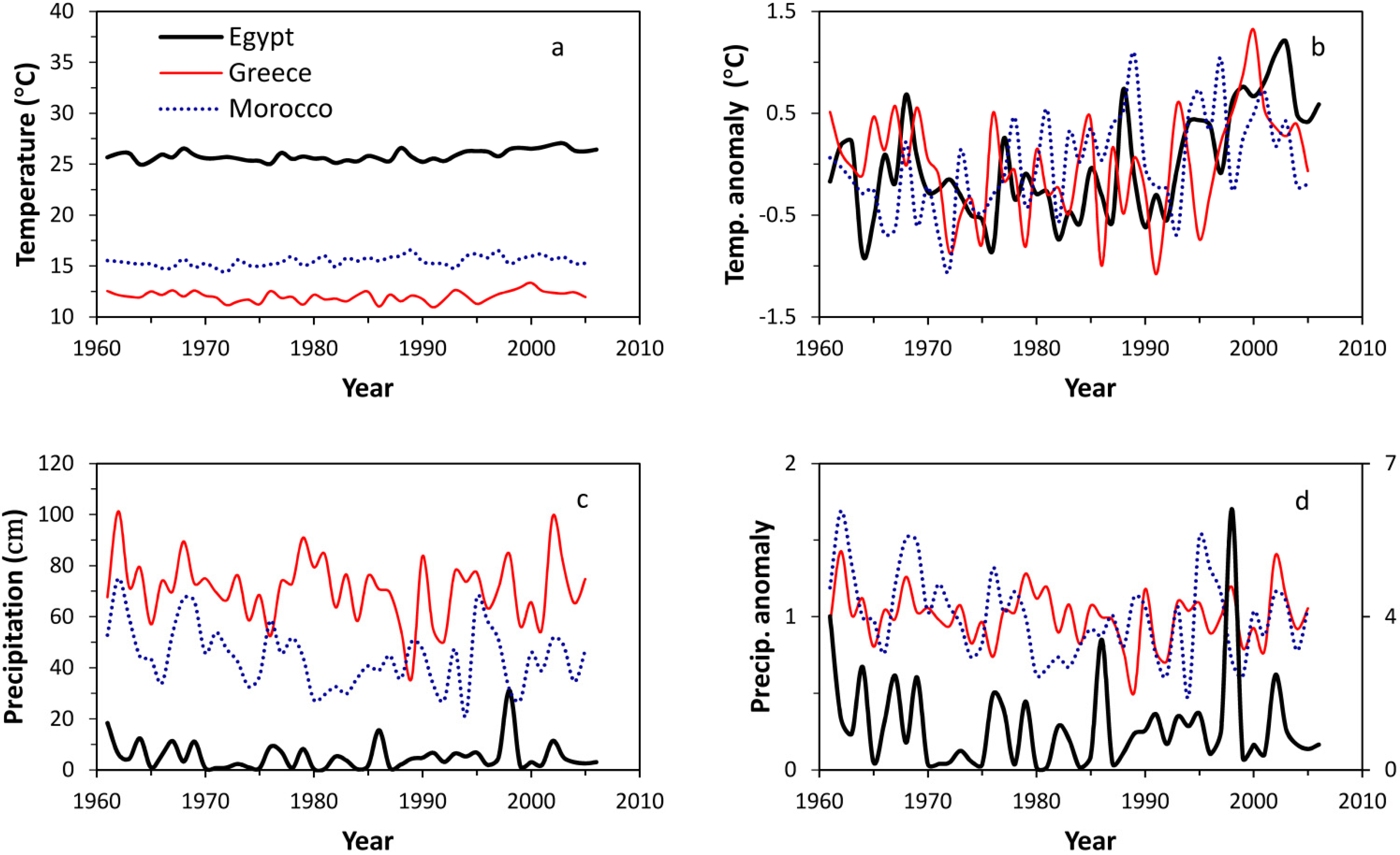
3.1. Climate


| 1961–2006 | 1971–2006 | p1/p2 | |
|---|---|---|---|
| Egypt | T = 0.014t − 6.56 | T = 0.026t − 30.28 | 9e4/~0 |
| P = 0.017t − 24.26 | P = 0.024t − 37.86 | 0.62/0.64 | |
| Greece | T = 0.0075t + 0.55 | T = 0.03t − 44.36 | 0.17/~0 |
| P = −0.0684t + 194.13 | P = −0.011t + 79.5 | 0.51/0.94 | |
| Morocco | T = 0.025t − 31.33 | T = 0.038t − 58.31 | 0/0 |
| P = −0.233t + 496.7 | P = −0.169t + 369.43 | 0.025/0.22 |
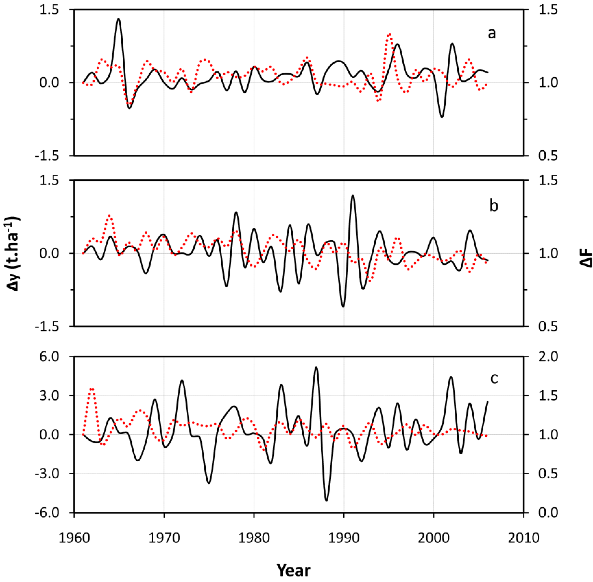
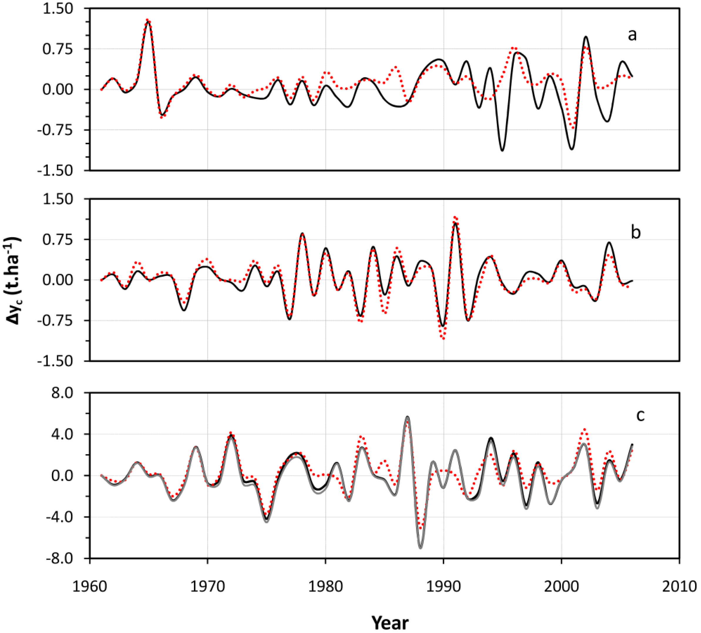
3.2. Crop Yield

| y = f(F,I) | R2 | p | |
|---|---|---|---|
| Maize—Egypt | y = −0.0304F3 + 0.4003F2 − 0.5656F + 0.9769 | 0.90 | <0.05 |
| Wheat—Greece | y = −0.1027F3 + 0.6308F2 − 0.6045F + 0.1372 | 0.70 | <0.05 |
| Potato—Morocco | y = (−0.0166F3 + 0.3029F2 − 0.9418F) + (28.3442I3 − 100.1485I2 +120.412I) − 48.1972 | 0.89 | ~0 |

3.2.1. Maize—Egypt

| Case Study | Y = f(time) |
|---|---|
| Maize—Egypt | |
| FDA | ∆yc = 0.00245.t − 4.78 |
| Our approach | ∆yc = −0.0011.t − 2.1423 |
| Wheat—Greece | |
| FDA | ∆yc = −0.0026.t + 5.3028 |
| Our approach | ∆yc = 0.0013.t − 2.5148 |
| Potato—Morocco | |
| FDA | ∆yc = 0.0177.t − 34.8 |
| Our approach (effect of F removed) | ∆yc = 0.0099.t − 19.531 |
| Our approach (effects of F & I removed) | ∆yc = 0.0086.t − 17.162 |
3.2.2. Wheat—Greece
3.2.3. Potato—Morocco
4. Discussion and Conclusion
Acknowledgments
Conflicts of Interest
References
- Fischer, G.; Shah, M.; Tubiello, F.N.; van Velhuizen, H. Socio-economic and climate change impacts on agriculture: An integrated assessment, 1990–2080. Philos. Trans. Roy. Soc. B 2005, 360, 2067–2083. [Google Scholar] [CrossRef]
- Burke, M.; Miguel, E.; Satyanath, S.; Dykema, J.; Lobell, D. Warming increases risk of civil war in Africa. Proc. Natl. Acad. Sci. USA 2009, 106, 20670–20674. [Google Scholar]
- Bloem, M.W.; Semba, R.D.; Kraemer, K. Castel Gangolfo workshop: An introduction to the impact of climate change, the economic crisis, and the increase in the food prices on malnutrition. J. Nutr. 2010, 140, 132–135. [Google Scholar] [CrossRef]
- Brinkman, H.-J.; de Pee, S.; Sanogo, I.; Subran, L.; Bloem, M.W. High food prices and the global financial crisis have reduced access to nutritious food and worsened nutritional status and health. J. Nutr. 2010, 140, 153–161. [Google Scholar] [CrossRef]
- Challinor, A.J.; Ewert, F.; Arnold, S.; Simelton, E.; Fraser, E. Crops and climate change: Progress, trends, and challenges in simulating impacts and informing adaptation. J. Exp. Bot. 2009, 60, 2775–2789. [Google Scholar] [CrossRef]
- Roudier, P.; Sultan, B.; Quirion, P.; Berg, A. The impact of future climate change on West African crop yields: What does the recent literature say? Glob. Environ. Chang. 2011. [Google Scholar] [CrossRef]
- Long, S.P.; Ainsworth, E.A.; Leakey, A.D.B.; Morgan, P.B. Global food insecurity. Treatment of major food crops with elevated carbon dioxide or ozone under large-scale fully open-air conditions suggests recent models may have overestimated future yields. Philos. Trans. Roy. Soc. B 2009, 360, 2011–2020. [Google Scholar]
- Lelieveld, J.; Hadjinicolaou, P.; Kostopolou, E.; Chenoweth, J.; El Maayar, M.; Giannakopoulos, C.; Hannides, C.; Lange, M.A.; Tanarhte, M.; Tyrlis, E.; et al. Climate change and impacts in the Eastern Mediterranean and the Middle East. Clim. Chang. 2012. [Google Scholar] [CrossRef]
- Palosuo, T.; Kersebaum, K.C.; Angulo, C.; Hlavinka, P.; Moriondo, M.; Olesen, J.E.; Patil, R.H.; Ruget, F.; Rumbaur, C.; Takáč, J.; et al. Simulation of winter wheat yield and its variability in different climates of Europe: A comparison of eight crop growth models. Eur. J. Agron. 2011. [Google Scholar] [CrossRef]
- Ainsworth, E.A.; Leakey, A.D.B.; Ort, D.R.; Long, S.P. FACE-ing the facts: Inconsistencies and interdependence among field, chamber and modeling studies of elevated CO2 impacts on crop yield and food supply. New Phytol. 2008, 179, 5–9. [Google Scholar] [CrossRef]
- El-Maayar, M.; Sonnentag, O. Crop model validation and sensitivity to climate change scenarios. Clim. Res. 2009, 39, 47–59. [Google Scholar] [CrossRef]
- Moriondo, M.; Giannakopoulos, C.; Bindi, M. Climate change impact assessment: The role of climate extremes in crop yield simulation. Clim. Chang. 2010, 104, 679–701. [Google Scholar]
- Rötter, R.P.; Carter, T.R.; Olesen, J.E.; Porter, J.R. Crop-climate models need an overhaul. Nat. Clim. Chang. 2011, 1, 175–177. [Google Scholar] [CrossRef]
- Lobell, D.B.; Burke, M.B. On the use of statistical models to predict crop yield responses to climate change. Agric. For. Meteorol. 2010. [Google Scholar] [CrossRef]
- Tubiello, F.N.; Ewert, F. Simulating the effects of elevated CO2 on crops: Approaches and applications for climate change. Eur. J. Agron. 2002, 18, 57–74. [Google Scholar] [CrossRef]
- El-Maayar, M.; Ramankutty, N.; Kucharik, C. Modelling global and regional net primary production under elevated atmospheric CO2: On a potential source of uncertainty. Earth Interact. 2006, 10, 1–20. [Google Scholar]
- Nicholls, N. Increased Australian wheat yield due to recent climate trends. Nature 1997, 387, 484–485. [Google Scholar] [CrossRef]
- Lobell, D.B.; Ortiz-Monasterio, J.I.; Asner, G.P.; Matson, P.A.; Naylor, R.L.; Falcon, W.P. Analysis of wheat yield and climatic trends in Mexico. Field Crop. Res. 2005, 95, 250–256. [Google Scholar]
- Lobell, D.B.; Field, C.B. Global scale climate-crop yield relationships and the impacts of recent warming. Environ. Res. Lett. 2007, 2. [Google Scholar] [CrossRef]
- Chaudhari, K.N.; Oza, M.P.; Ray, S.S. Impacts of Climate Change on Yields of Major Food Crops in India. In Proceedings of ISPRS Archives XXXVIII-8/W3 Workshop Impact of Climate Change on Agriculture, Ahmedabad, India, 17–18 December 2010; pp. 100–105.
- Osborn, T.M.; Wheeler, T.R. Evidence for a climate signal in trends of global crop yield variability over the past 50 years. Environ. Res. Lett. 2013, 8. [Google Scholar] [CrossRef]
- Peltonen-Sainio, P.; Jauhiainen, L.; Trnka, M.; Olesen, J.E.; Calanca, P.L.; Eckersten, H.; Eitzinger, J.; Gobin, A.; Kersebaum, K.C.; Kozyra, J.; et al. Coincidence of variation in yield and climate in Europe. Agric. Ecosyst. Environ. 2010, 139, 483–489. [Google Scholar] [CrossRef]
- Brisson, N.; Gate, P.; Gouache, D.; Charmet, G.; Oury, F-X.; Huard, F. Why are wheat yields stagnating in Europe. Field Crop. Res. 2010, 119, 201–212. [Google Scholar] [CrossRef]
- Cassman, K.G.; Dobermann, A.; Walters, D.T. Agroecosystems, nitrogen-use efficiency, and nitrogen management. AMBIO. 2002, 31, 132–140. [Google Scholar]
- Chloupek, O.; Hrstkova, P.; Schweigert, P. Yield and its stability, crop diversity, sdaptability and response to climate change, weather and fertilisation over 75 years in the Czech Republic in comparison to some countries. Field Crop. Res. 2004, 85, 167–190. [Google Scholar] [CrossRef]
- Donner, S.D.; Kucharik, C.J. Evaluating the impacts of land management and climate variability on crop production and nitrate export across the Upper Mississippi Basin. Glob. Biogeochem. Cy. 2003, 17. [Google Scholar] [CrossRef]
- Schlenker, W.; Lobell, D.B. Robust negative impacts of climate change on African agriculture. Environ. Res. Lett. 2010, 5, 1–8. [Google Scholar]
- Long, S.P.; Ainsworth, E.A.; Leakey, A.D.B.; Nösberger, J.; Ort, D.R. Food for thought: Lower-than-expected crop yield stimulation with rising CO2 concentrations. Science 2006, 312, 1918–1921. [Google Scholar] [CrossRef]
- Devaney, R.L.; Hall, G.R. Differential Equations, 4th ed.; Brooks-Cole Publ. Co.: Pacific Grove, California, CA, USA, 2006. [Google Scholar]
- Food and Agriculture Organization of the United Nations (FAO) statistical Databases. Available online: http://faostat.fao.org/site/567/default.aspx#ancor (accessed on 16 April 2012).
- Mitchell, T.D.; Jones, P.D. An improved method of constructing a database of monthly climate observations and associated high-resolution grids. Int. J. Climatol. 2005, 25, 693–712. [Google Scholar] [CrossRef]
- Leff, B.; Ramankutty, N.; Foley, J.A. Geographic distribution of major crops across the world. Glob. Biogeochem. Cy. 2004, 18. [Google Scholar] [CrossRef]
- Monfreda, C.; Ramankutty, N.; Foley, J.A. Farming the planet: 2. Geographic distribution of crop areas, yields, physiological types, and net primary production in the year 2000. Glob. Biogeochem. Cy. 2008, 22. [Google Scholar] [CrossRef]
- IFA. International Fertilizer Association (IFA) Database. Available online: http://www.fertilizer.org/ifa/ifadata/search (accessed on 16 April 2012).
- Freydank, K.; Siebert, S. Towards Mapping the Extent of Irrigation in the Last Century: Time Series of Irrigated Area Per Country; Frankfurt Hydrology Papper 08; Institute of Physical Geography, University of Frankfurt: Frankfurt am Main, Germany, April 2008. [Google Scholar]
- Oenema, O.; Pietrzak, S. Nutrient management in food production: Achieving agronomic and environmental targets. AMBIO 2002, 31, 159–168. [Google Scholar]
- Lopes, A.S.; Guilherme, L.R.G.; da Silva, C.A.P. Vocação da terra, 2nd ed.; ANDA: São Paulo, Brazil, 2003; p. 23. [Google Scholar]
- Sacks, W.J.; Deryng, D.; Foley, J.A.; Ramankutty, N. Crop planting dates: An analysis of global patterns. Glob. Ecol. Biogeogr. 2010, 19, 607–620. [Google Scholar]
- Intergovernmental Panel on Climate Change (IPCC), Climate Change 2007: The Physical Science Basis. In Contribution of Working Group I to the Fourth Assessment Report of the Intergovernmental Panel on Climate Change; Solomon, S. (Ed.) Cambridge University Press: Cambridge, UK, 2007.
- Giannakopoulos, C.; Le Sager, P.; Bindi, M.; Moriondo, M.; Kostopoulou, E.; Goodess, C.M. Climatic changes and associated impacts in the Mediterranean resulting from global warming. Glob. Planet. Chang. 2009, 68, 209–224. [Google Scholar] [CrossRef]
- Monteith, J.L. Presidential address to the royal meteorological society. Qua. J.Roy. Meteor. Soc. 1981, 107, 749–774. [Google Scholar] [CrossRef]
- Sage, R.; Pearcy, R.W. The Physiological Ecology of C4 Photosynthesis. Adv. Photosyn Resp. 2004, 9, 497–532. [Google Scholar] [CrossRef]
- Alpert, P.; Ben-Gai, T.; Baharad, A.; Benjamini, Y.; Yekutieli, D.; Colacino, M.; Diodato, L.; Ramis, C.; Homar, V.; Romero, R.; et al. The paradoxical increase of Mediterranean extreme daily rainfall in spite of decrease in total values. Geophys. Res. Lett. 2002, 29. [Google Scholar] [CrossRef]
© 2013 by the authors; licensee MDPI, Basel, Switzerland. This article is an open access article distributed under the terms and conditions of the Creative Commons Attribution license (http://creativecommons.org/licenses/by/3.0/).
Share and Cite
El-Maayar, M.; Lange, M.A. A Methodology to Infer Crop Yield Response to Climate Variability and Change Using Long-Term Observations. Atmosphere 2013, 4, 365-382. https://doi.org/10.3390/atmos4040365
El-Maayar M, Lange MA. A Methodology to Infer Crop Yield Response to Climate Variability and Change Using Long-Term Observations. Atmosphere. 2013; 4(4):365-382. https://doi.org/10.3390/atmos4040365
Chicago/Turabian StyleEl-Maayar, Mustapha, and Manfred A. Lange. 2013. "A Methodology to Infer Crop Yield Response to Climate Variability and Change Using Long-Term Observations" Atmosphere 4, no. 4: 365-382. https://doi.org/10.3390/atmos4040365