Article

Biomass Burning Aerosols Observed in Northern Finland during the 2010 Wildfires in Russia

1
Kuopio Unit, Finnish Meteorological Institute, P.O. Box 1627, FI-70211 Kuopio, Finland
2
Climate Change, Finnish Meteorological Institute, P.O. Box 503, FI-00101 Helsinki, Finland
3
Arctic Research, Finnish Meteorological Institute, Tähteläntie 62, FI-99600 Sodankylä, Finland
*
Author to whom correspondence should be addressed.
Atmosphere 2013, 4(1), 17-34; https://doi.org/10.3390/atmos4010017
Submission received: 31 October 2012 / Revised: 4 February 2013 / Accepted: 19 February 2013 / Published: 28 February 2013

Abstract

:
A smoke plume originating from the massive wildfires near Moscow was clearly detected in northern Finland on 30 July 2010. Measurements made with remote sensing instruments demonstrated how the biomass burning aerosols affected the chemical and optical characteristics of the atmosphere in regions hundreds of kilometers away from the actual fires. In this study, we used MODIS, AIRS, CALIOP, PFR, ceilometers, FTS and Brewer data to quantify the properties of the transported smoke plume. In addition, in situ measurements of aerosol concentration (DMPS), absorption (aethalometer) and scattering (nephelometer) are presented. We found that due to the smoke plume in northern Finland, the daily averaged optical thickness of aerosols increased fourfold, and MODIS retrieved AOD as high as 4.5 for the thickest part of the plume. FTS measurements showed that CO concentration increased by 100% during the plume. CALIOP and ceilometer measurements revealed that the smoke plume was located close to the surface, below 3 km, and that the plume was not homogeneously mixed. In addition, in situ measurements showed that the scattering and absorption coefficients were almost 20 times larger in the smoke plume than on average, and that the number of particles larger than 320 nm increased 14-fold. Moreover, a comparison with in situ measurements recorded in eastern Finland on the previous day showed that the transport from eastern to northern Finland decreased the scattering coefficient, black carbon concentration, and total number concentration 0.5%/h, 1.5%/h and 2.0%/h, respectively.

1. Introduction

Intensive wildfires took place in the western parts of Russia, near Moscow, during June–August 2010. In addition to the destruction caused by the fires, massive amounts of biomass-burning-derived aerosols were released into the atmosphere. The smoke from the fires and associated aerosol particles reduced the air quality considerably in the western part of Russia and neighboring countries. The smoke drifted long distances with air masses, and during several days, it could be clearly observed in eastern and northern parts of Finland.
During the summer of 2010, Eastern Europe and large parts of Russia experienced a “mega-heat wave” [1]. The daily temperature in Moscow reached 38.2 °C at maximum and the nighttime temperature in Kiev stayed at 25 °C during the warmest night. Due to the heat wave, approximately 55,000 people died in Russia. Hot and dry conditions were ideal for extensive wildfires, which resulted in 1 million ha of burned areas [1]. Several studies concerning these wildfires and their emissions have already been published. Witte [2] presented an extensive study on the impact of wildfire emissions on the atmospheric composition during the heat wave, based on observations performed with instruments on board NASA satellites. Mei [3] combined remote sensing data and surface observations to estimate the impacts of the wildfires over Europe and Asia. They found that in a number of Eastern European countries (including Finland) the particle mass concentrations were enhanced by a factor of 3–5 on the days when wildfire plumes moved westward. Yurganov [4] presented carbon monoxide (CO) total column observations from ground-based and spaceborne instruments. They assessed that the total CO emitted by the Russian fires was between 34 and 40 Tg during July–August 2010. Van Donkelaar [5] estimated daily mean fine particulate matter (PM2.5) concentrations by using The Moderate Resolution Imaging Spectroradiometer (MODIS), Aerosol Optical Depth (AOD) data, and the GEOS-Chem chemical transport model to reach values as high as 600 µg·m−3 during the fire episode. Konovalov [6] analyzed surface concentrations of CO, particle mass (PM10) and ozone in the Moscow region using remote sensing and ground-based measurements with a mesoscale model. They concluded that the extreme air pollution episodes in Moscow were mainly caused by fires less than 200 km away. However, they also showed that, periodically, the wildfires degraded air quality further away in Eastern and Northern Europe.
The transport of biomass burning emissions is an important topic, especially for the arctic regions. Warneke [7] showed that fires in Russia can more than double the high seasonal Arctic atmospheric background burden. Moreover, Barnaba [8] found that fires in Russia and Eastern Europe increase the fine fraction AOD in Europe during most of the year, especially in the spring. The most impacted regions are Eastern and Central Europe, as well as the northern countries. The transport and properties of the biomass burning plumes advected to Finland during the 2010 Russian fires have been studied by Portin [9] and Mielonen [10]. They found significant increases in particle mass, size, AOD and amount of black carbon.
In this paper, observations of biomass burning plumes originating from the 2010 Russian wildfires are presented from two measurement sites in northern Finland: Sodankylä and Pallas. Although a number of articles have been published concerning this wildfire event (e.g., [1,2,3,4,5,6,9,10]), these are the first published results from Arctic measurement stations. Smoke aerosols are especially important in the Arctic because they have a considerable effect on surface albedo when they deposit on snow, and they introduce significant increases to the typically very low aerosol concentrations [11].

2. Instrumentation

To study the properties of the transported smoke plume, we used measurements from ground-based Precision Filter Radiometer (PFR), Brewer, ceilometers and Fourier Transform Spectrometer (FTS). The ground-based instruments are located in Sodankylä (67.368°N, 26.633°E) and Pallas (67.967°N, 24.117°E). Moreover, spaceborne instruments such as Moderate Resolution Imaging Spectroradiometer (MODIS), Atmospheric Infrared Sounder (AIRS) and Aerosol Lidar with Orthogonal Polarization (CALIOP) are used in the analysis of the plumes. In addition to remote sensing measurements, we used in situ measurements of carbon monoxide, carbon dioxide, aerosol concentration, absorption and scattering coefficients taken at Pallas.

2.1. Remote Sensing Measurements

2.1.1. PFR

The Precision Filter Radiometer (PFR, [12,13]) is a passive instrument which measures direct solar irradiance in four narrow spectral bands (368, 412, 500, and 862 nm). The bandwidth of the instrument is 5 nm, and the full field of view angle is 2.5 degrees. Derived products from the measurements are Aerosol Optical Depth (AOD) for the four wavelengths and Ångström exponent (AE). The time resolution of the products is 1 min. The absolute uncertainty in the AOD values of the PFR instrument are between 0.01 and 0.02 [14]. Cloud screening of the PFR measurements is based on the method presented by Smirnov [15]. The instrument used in this study is located at Sodankylä.

2.1.2. Brewer

The Brewer network consists of about 200 spectrophotometers [16] making measurements in the UV-B radiation band. AOD can be retrieved from these instruments using the Langley Plot Method (LPM) [17]. The development and description of the method has been published in several papers (e.g., [18,19,20,21]). In addition, several validation studies concerning the accuracy of the AOD in the UV-B region have also been conducted (e.g., [22,23,24]). The Brewer instrument used in this study is located at Sodankylä.

2.1.3. FTS

Fourier Transform Spectrometer (FTS, [25,26]) measures atmospheric columns of various gases by using the spectrum of direct solar radiation. The FTS used in this study is a Bruker IFS 125 HR instrument with A547N Solar Tracker, located in Sodankylä. The instrument has three detectors with the following wave number ranges: Si-diode detector (25,000–9,000 cm−1), InGaAs detector (12,800–4,000 cm−1) and InSb detector (9,600–1,850 cm−1); the spectral resolution is approximately 0.02 cm−1. The instrument is participating in the Total Carbon Column Observing Network (TCCON), which is a ground-based network designed to retrieve precise and accurate column abundances of CO2, CH4, CO, N2O, H2O, HDO, O2, and HF from near-infrared solar absorption spectra [27]. Here the TCCON algorithms have been used to compute CO column abundances from the FTS measured spectra.

2.1.4. MODIS

The Moderate Resolution Imaging Spectroradiometer (MODIS, [28]) is one of the most widely used passive satellite instruments in aerosol remote sensing. There are two MODIS instruments which are on board the Terra and Aqua satellites. Having a swath width of 2,300 km, both instruments cover the earth’s surface every 1 to 2 days. Beginning in early 2007, a consistent algorithm [29] was used to process the entire MODIS data record, providing the so-called Collection 5 data set. Levy [29] (and the on-line Algorithm Theoretical Basis Document, ATBD) have provided a detailed documentation of the algorithm.
MODIS Collection 5 data from both satellites are used in the comparisons with the ground-based measurements. The expected error over land in the MODIS AOD is ±0.05 ± 0.15 × AOD [30]. We used level 2 AOD data, which has a spatial resolution of 10 × 10 km2 at nadir. Only AOD data with best quality (Quality flag = 3) were considered in the analysis [30]. For the comparisons with sun photometer measurements, we used the Optical_Depth_Land_And_Ocean product. The data were downloaded from MODIS L1 and Atmospheres Archive and Distribution System (LAADS) Web [31]. We also used level 3 data from the Giovanni web page [32] to study the shape of the biomass burning plume.
In addition to aerosol data, we used MODIS Fire Radiative Power (FRP) data to locate fires and study their intensity. These data are available at the Fire Information for Resource Management System (FIRMS, [33]).

2.1.5. AIRS

The Atmospheric Infrared Sounder (AIRS, [34,35]) is on board the Aqua satellite (with MODIS) and part of the A-Train constellation. It provides very high spectral resolution measurements of emitted radiation in three spectral bands (3.74–4.61 µm, 6.20–8.22 µm and 8.80–15.40 µm) using 2,378 channels. In addition, four channels in the visible/near infrared observe wavelengths between 0.4 and 1 µm to characterize cloud cover and spatial variability. The spatial resolution of the measurements is 13.5 km at nadir. AIRS standard products include temperature, water vapor mixing ratios and trace gas concentrations (e.g., O3, CO, CO2, CH4). In this study, we used level 3 daily carbon monoxide (CO) data from the ascending orbit which has a spatial resolution of 1 × 1 degree. The data are available from Giovanni [36].

2.1.6. CALIOP

The Cloud-Aerosol Lidar and Infrared Pathfinder Satellite Observation (CALIPSO, [37,38]) satellite was launched in April 2006, and data has been available from June 2006 onward. CALIPSO carries the Cloud-Aerosol Lidar with Orthogonal Polarization (CALIOP) instrument, which can measure the vertical structure of the atmosphere at three channels, from the intensity of that part of the (pulsed) laser light that is scattered back to the lidar receiver. Two of these channels, at 532 nm, are orthogonally polarized, and one channel measures the total backscattered signal at 1,064 nm. The diameter of the laser pulse at ground level is about 70 m. CALIOP has a spatial resolution of 333 m along the orbital path. The satellite repeat cycle is 16 days [39]. We used level 2, version 3.1, aerosol profile products (backscattering and extinction at 532 nm) in the analysis.

2.1.7. Ceilometers

Both Sodankylä and Pallas have Vaisala CT25K ceilometers [40,41], which can be used to retrieve the altitude of aerosol layers even though the instruments are originally designed to measure cloud heights. The Vaisala single-lens ceilometer CT25K provides the attenuated backscatter intensity profiles at a wavelength of 905 nm up to 7.5 km. In addition to cloud height measurements, it has been used, for example, in the detection of the mixing layer height [42].

2.2. In situ Measurements

Ground-based in situ aerosol measurements were conducted in Pallas, at the top of Sammatunturi hill (565 m ASL). The station is part of Pallas-Sodankylä Global Atmosphere watch station. It is located some 130 km northwest of Sodankylä. A detailed site description can be found in [43]. The scattering and backscattering coefficients were measured with an integrating nephelometer (model 3563, TSI, Inc., St. Paul, MN, USA). Aaltonen [44] has described the nephelometer measurements and data processing in more detail. The absorption coefficient was measured with Aethalometer (Magee Scientific, model AE31). A more detailed description of the Aethalometer measurements and data processing can be found in [45]. The size distribution is measured with a Differential Mobility Particle Size (DMPS). It measures the number size distribution between 7 and 500 nm. See [46] for a more detailed description of DMPS measurements and data processing. CO2 was measured with a Picarro G1301 CRDS (Cavity Ring-Down-Spectroscopy) analyzer and CO with a Gas Chromatograph/Reduction Gas Detector. These measurements are described in more detail by Hatakka [43]. The CO and CO2 data were used to calculate the modified combustion efficiency (MCE, [47])
Atmosphere 04 00017 i001
where ΔCO and ΔCO2 are the excess molar mixing ratios of CO and CO2 for the smoke plumes. In order to calculate these excess quantities, we assumed that the ambient concentrations of CO and CO2 were equal to the minimum value measured in July 2010. MCE can be used to distinguish between flaming and smoldering combustion. When MCE is larger than 0.9 the emissions are from flaming combustion; when it is below 0.9, the combustion is thought to be smoldering [48].

3. Results and Discussion

On 30 July 2010, a smoke plume originating from the Russian wildfires was detected, with a number of instruments, in northern Finland (Sodankylä and Pallas). Sodankylä and Pallas are typically very pristine locations and therefore the plume day is clearly visible in the measurements. As Figure 1(a) shows, the air mass trajectories calculated with Hybrid Single Particle Lagrangian Integrated Trajectory Model (HYSPLIT, [49,50,51]) that reach Sodankylä during that day are mainly originating from the wildfire region. The MODIS level 3 AOD data in Figure 1(b) shows how the smoke plume with AODs up to 4 reached Sodankylä, while the rest of Finland remained relatively unaffected by the plume.
Figure 1. (a) air mass trajectories at three levels (500 m ASL (green), 1,000 m (blue), 3,000 m (magenta)) for 30 July and the fires detected by MODIS on 28 July (yellow), 29 July (red) and 30 July (black). The trajectories are for 48 h and the time difference between the symbols is six hours. (b) daily averaged AOD (level 3) from MODIS (Aqua) for 30 July. (c) AIRS (Aqua) total CO concentration (1018 molecules/cm2, level 3) on 30 July 2010.
Atmosphere 04 00017 g001
The total column CO values retrieved from AIRS measurements show an even more detailed picture of the plume (Figure 1(c)). The maximum CO values are as high as 5 × 10¹⁸ molecules/cm2, which is slightly larger than the values in the plumes detected in Eastern Finland during this episode (3.2–4.5 × 10¹⁸ molecules/cm2, [10]).
Enhanced CO values on the 30 July were also measured in Sodankylä with a FTS instrument. Figure 2 shows that the daily average column abundance of CO was 3.41 × 10¹⁸ molecules/cm2 on 30 July, while typical values are around 1.7 × 10¹⁸ molecules/cm2. Thus, the smoke plume doubled the amount CO in this region. The maximum value on 30 July was 5.32 × 10¹⁸ molecules/cm2. This is the highest column abundance of CO measured since the start of the FTS measurements in Sodankylä in February 2009. The FTS measurements also showed enhanced CO values on 26 July (1.96 × 10¹⁸ molecules/cm2) and on 27 July (2.3 × 10¹⁸ molecules/cm2). This implies that some smoke reached northern Finland also then. On 28 and 29 July, FTS was not able to do measurements due to cloudiness.
Figure 2. Daily averaged CO column abundance (thick solid line) and +/− one standard deviation per day derived from the individual measurements (dotted lines) at Sodankylä with the FTS instrument.
Atmosphere 04 00017 g002
Figure 3 presents a time series of CO2 and CO mixing ratios measured at the Pallas site. Typically, CO is a better indicator for biomass burning plumes than CO2 because CO2 is constantly emitted from anthropogenic sources. However, the CO2 data shows a small peak (405 ppm) during the night between 27 and 28 July. The CO data also has a peak (180 ppb) at the same time. In addition, CO data has a peak (160 ppb) on 30 July. Enhanced CO values were also detected at Sodankylä on the same days, as discussed above (Figure 2).
Figure 3. Time series of CO2 and CO measured in situ at Pallas site.
Atmosphere 04 00017 g003
Based on the in situ CO and CO2 measurements, we calculated the modified combustion efficiency (MCE) to see if there is a difference between the two plume days. As Figure 4 shows, the MCE value for the plume on 27 July is 0.66, while on 30 July, the values are over 0.9. This indicates that the plume on 30 July was from flaming combustion while the plume on 27 July was from smoldering combustion. Moreover, low MCE values (<0.7) are associated with peat fires [52], thus confirming that the smoke on 27 July was from the peat fires in Russia [6].
Figure 4. Time series of MCE at Pallas site.
Atmosphere 04 00017 g004
The daily averaged AOD measurements from the MODIS, PFR and Brewer instruments are shown in Figure 5. MODIS and PFR are measuring in the visible and Brewer measures in the UV. All instruments show a dramatic increase in AOD during 30 July with around four times larger values than usual. Mei [3] reported similar increases in AOD during this episode. Typically, the AOD values in Sodankylä (measured with PFR) are around 0.08, therefore, the increase to 0.6 is already a significant change. However, as Figure 6 illustrates, the daily averaged PFR AOD value is based on measurements from the morning and the afternoon, thus, the largest impact of the plume is missed, due to strict cloud screening. MODIS, on the other hand, has a measurement also from the thickest smoke plume (AOD up to 4.5). This explains the large difference in the daily averaged AOD values for 30 July. MODIS and PFR measured almost simultaneously at around 9 a.m. UTC and show excellent agreement (Figure 5). Mielonen [10] presented MODIS AOD values from around 1 p.m. from eastern Finland (Kuopio) on the previous day (29). This indicates that the thickest part of the smoke plume did not reach Kuopio that day, but it passed Kuopio from the north and arrived at Sodankylä on the following day. Figure 4 also shows that MODIS and Brewer detected enhanced AOD values on 27 July (PFR did not measure during this day), thus indicating that there might have been some smoke in Sodankylä on that day as well. The enhanced CO mixing ratios measured at Sodankylä and Pallas during the same day and the following night support this conclusion.
Figure 5. Daily averaged AOD values for Sodankylä from three instruments: PFR (500 nm), Brewer (320 nm) and MODIS (550 nm).
Atmosphere 04 00017 g005
Figure 6. AOD values measured in Sodankylä with PFR (500 nm), and MODIS (550 nm) on 30 July 2010.
Atmosphere 04 00017 g006
In order to get information on the vertical distribution of the smoke plumes, we used CALIOP measurements. On 30 July, CALIOP flew twice in the proximity of Sodankylä. The distances of the night overpass (at 1:11 a.m. UTC) and the day overpass (10:53 a.m. UTC) were 76 km and 146 km, respectively. The extinction, backscattering and lidar ratio profiles (532 nm) presented in Figure 7 show that on the night of 30 July the aerosols were situated in multiple layers: two thin layers below 1 km, a thicker layer from 1 km to 2 km and, possibly, two thin layers between 2 and 4 km. The lidar ratios for the layers below 2 km are close 60 sr, which indicates a mixture of biomass burning aerosols (lidar ratio of 70 sr in the CALIOP retrieval) and other less absorbing aerosols (e.g., clean continental (35 sr), desert dust (40 sr), or polluted dust (55 sr)). For the day overpass, CALIOP detects only two aerosol layers: below and over 2 km. The lower layer has a lidar ratio of 70 sr, thus it contains solely biomass burning aerosols, while the upper layer’s lidar ratio of 55 sr indicates the presence of polluted dust. Dust aerosols are rarely detected in Finland; it therefore seems that the CALIOP retrieval has misclassified smoke as polluted dust. It is also worth noting that the night and day extinction profiles are similar, thereby indicating that the smoke plume did not change significantly between the measurements. AOD can be calculated from the extinction profile by integrating the extinction values. For the night profile, this results in an AOD of 0.45 which is significantly lower than the daily averaged value of 2 measured with MODIS, but closer to the value of 0.6 measured with PFR. The reason for this could be the time difference between the measurements and the relatively small dimensions of the plume. The daily profile has only two layers and their combined AOD is only around 0.1.
Figure 7. The average extinction, backscattering, and lidar ratio profiles on 30 July 2010. Nighttime measurements (at 1:11 a.m. UTC) in red, and daytime measurements (at 10:53 a.m. UTC) in blue. The measurements were done between latitudes 67.0 and 67.5.
Atmosphere 04 00017 g007
Ceilometers situated in Sodankylä and Pallas (Kenttärova station) also detected the biomass burning plume on 30 July. Figure 8 shows a time series of the attenuated backscatter coefficients on this day from both sites. The upper plot from Pallas shows that backscattering at altitudes below 1 km increases significantly between 2 p.m. and 6 p.m. (UTC). This coincides with the changes in the aerosol properties detected with in situ measurements done at Pallas (see the following paragraph). In Sodankylä (the lower plot in Figure 8), the plume is clearly visible from midnight until afternoon. More precisely, the plume was already detected on the previous night at 9 p.m. (UTC) (not shown in Figure 8). For the entire time, the plume is situated close to the surface, below 2 km, which is in good agreement with the CALIOP measurements. All the profile measurements show layers in the plume, thus indicating that it is not homogeneously mixed.
Figure 8. Time series of the attenuated backscatter coefficient measured with ceilometers on 30 July 2010 in Pallas (upper plot) and Sodankylä (lower plot).
Atmosphere 04 00017 g008
The smoke plume from the Russian wildfires was also observed with in situ measurements at the Pallas station on 30 July 2010. The main station was inside a cloud until midday. A few hours after midday, the wind direction changed quite rapidly from northeast to southeast, and all the aerosol properties changed significantly. In Figure 9, the absorption and scattering coefficients at the wavelength of 550 nm are presented for 30 July. The average of the scattering coefficient in July was 12 Mm−1 with a standard deviation of 18 Mm−1 and, during the plume, the one-hour average scattering coefficient increased up to 180 Mm−1. The average absorption coefficient during July was 0.9 Mm−1 with a standard deviation of 1.3 Mm−1, whereas, in the plume, the maximum one-hour average was 15 Mm−1. In the equivalent black carbon concentration, this maximum corresponds to about 900 ng·m−3. The single scattering albedo (SSA) varied only a little: 0.90 at scattering and absorption coefficient maximum, and 0.95 before the change in wind direction. The July average for SSA is 0.93. The measured SSA for the smoke plume sounds reasonable because it is in the same range as the values measured in Kuopio during the same smoke episode. The value is also in agreement with the SSA values for aged smoke measured in Europe and North America [53].
The aerosol scattering and absorption coefficients are clearly higher than the typical values in July also on 27 July: 45 and 3.5 Mm−1, respectively. This is in spite of the fact that the clouds and rain are contaminating the data and they cannot be directly compared to the measurements made on 30 July. On 29 July, there is also a short peak in the scattering coefficients (50 Mm−1), but the absorption coefficient from the aethalometer (0.6 Mm−1) is clearly lower than on 27 and 30 July. Unfortunately, clouds and rain are contaminating the data also on 29 July, and cloud-free data exist only for an order of an hour.
Figure 9. Scattering and absorption coefficients at a wavelength of 550 nm 30 July 2010. Grey horizontal bar indicates the time that the station was inside a cloud. Time is UTC + 2.
Atmosphere 04 00017 g009
In Figure 10(a), the total number concentration (D > 7 nm) and number concentrations in several different cut-off sizes (>100, >200, and >320 nm) are presented for 30 July 2010. The total average concentration in July 2010 was 1,420 cm−3 with a standard deviation of 1,130 cm−3. At the peak of the plume, the total concentration is only slightly higher, about 1,700 cm−3, while the optical properties increased almost 20-fold. Comparing the number concentration of particles larger than 100, 200 and 320 nm to July’s averages, the increases are 5, 8 and 14-fold, respectively. This clearly indicates that the number of larger particles is dominating in the plume compared to average values. This can also be observed from the size distributions in Figure 10(b). The number size distribution in the plume is clearly dominated by accumulation mode particles, whereas the size distribution in the average situation is dominated by smaller particles. Geometric mean diameter in the plume, 138 nm, is over twice as large as in the average size distribution, 58 nm. Usually the particle sizes that can act as cloud condensation nuclei are assumed to be particles larger than 100 nm. In Pallas, also slightly smaller particles can activate to cloud droplets [54]. The fact that the plume increases the number of particles larger than 100 nm indicates the ability of smoke plume aerosols to change the properties of clouds in the area.
These in situ results are in good agreement with the results presented by Portin [9] for eastern Finland (Kuopio) during the same episode. This was expected, because the plume that reached Sodankylä and Pallas on 30 July passed Kuopio on 29 July. Portin [9] reported about 20 times larger absorption and scattering coefficients and a stronger increase in the amount of larger particles. The absolute amount of particles and black carbon were larger in Kuopio than in northern Finland, which indicates that removal processes affected the plume during the transport. For the plume detected in Kuopio, the one-hour average scattering coefficient increased up to 213 Mm−1, which means that during the transport of 29 h to northern Finland, the scattering coefficient decreased 1 Mm−1/h, which equals to 0.5 %/h. The one-hour average black carbon concentration was 1,590 ng·m−3 in Kuopio, and the decrease during transport was 24 ng·m−3/h or 1.5 %/h. However, an even greater change was observed in the total number concentration. In Kuopio, the plume had an hourly average aerosol concentration of 5,030 cm−3, which decreased 115 cm−3/h or 2.0 %/h during transport. Likely, the actual rates are even larger because the Kuopio measurements were taken at the edge of the plume, while the Pallas measurements were made at the center of the plume.
Figure 10. (a) Number concentration of different size particles measured with DMPS on the 30 July 2010. Grey horizontal bar indicates the time that the station was inside a cloud. (b) Aerosol number size distributions during the smoke plume and on average in July 2010.
Atmosphere 04 00017 g010

4. Conclusions

The smoke plumes originating from the wildfires near Moscow in July–August 2010 had a considerable effect on the chemical and optical characteristics of the atmosphere in western Russia and northern/eastern Finland. In northern Finland, the smoke plumes were easily detected on 27 and 30 July 2010. Measurements made with remote sensing and in situ instruments clearly showed how the biomass burning aerosols affected the chemical and optical characteristics of the atmosphere in regions hundreds of kilometers away from the actual fires. In this study, we used MODIS, AIRS, CALIOP, PFR, FTS, Brewer, ceilometer, DMPS, gas analyzers, aethalometer and nephelometer data to quantify the properties of the smoke plume. We found that:
(1)
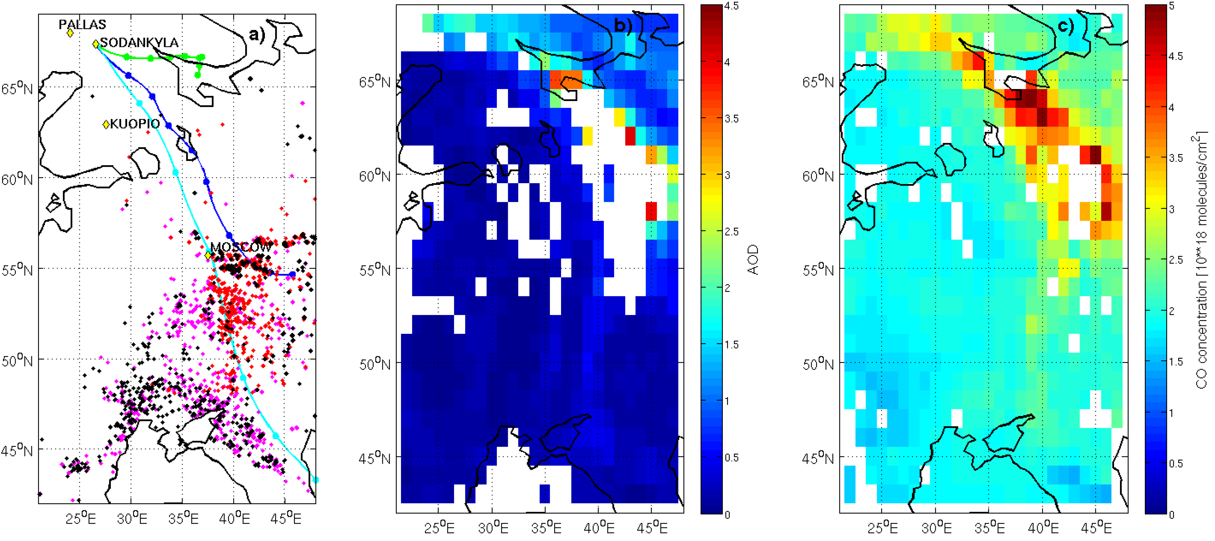
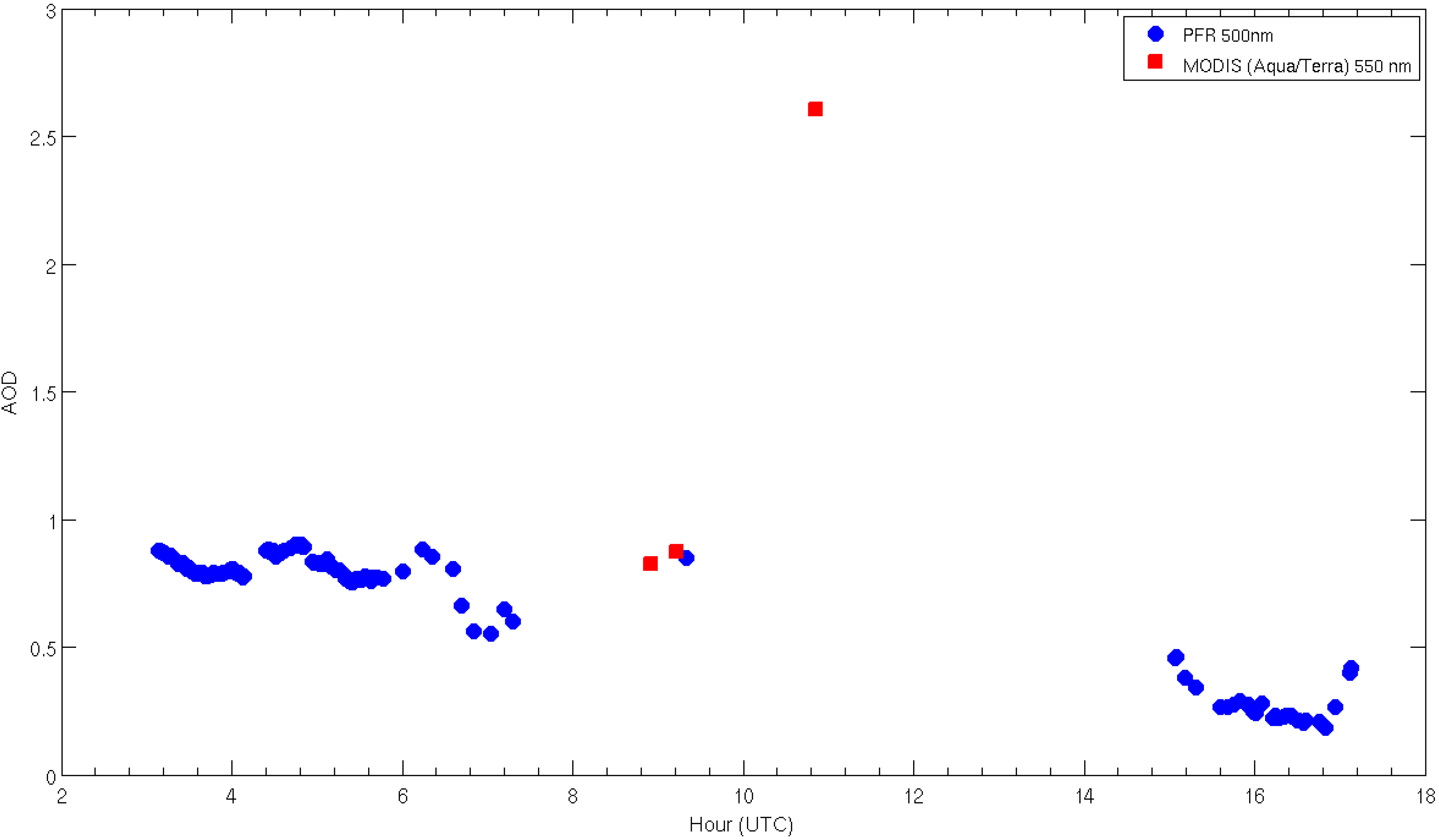
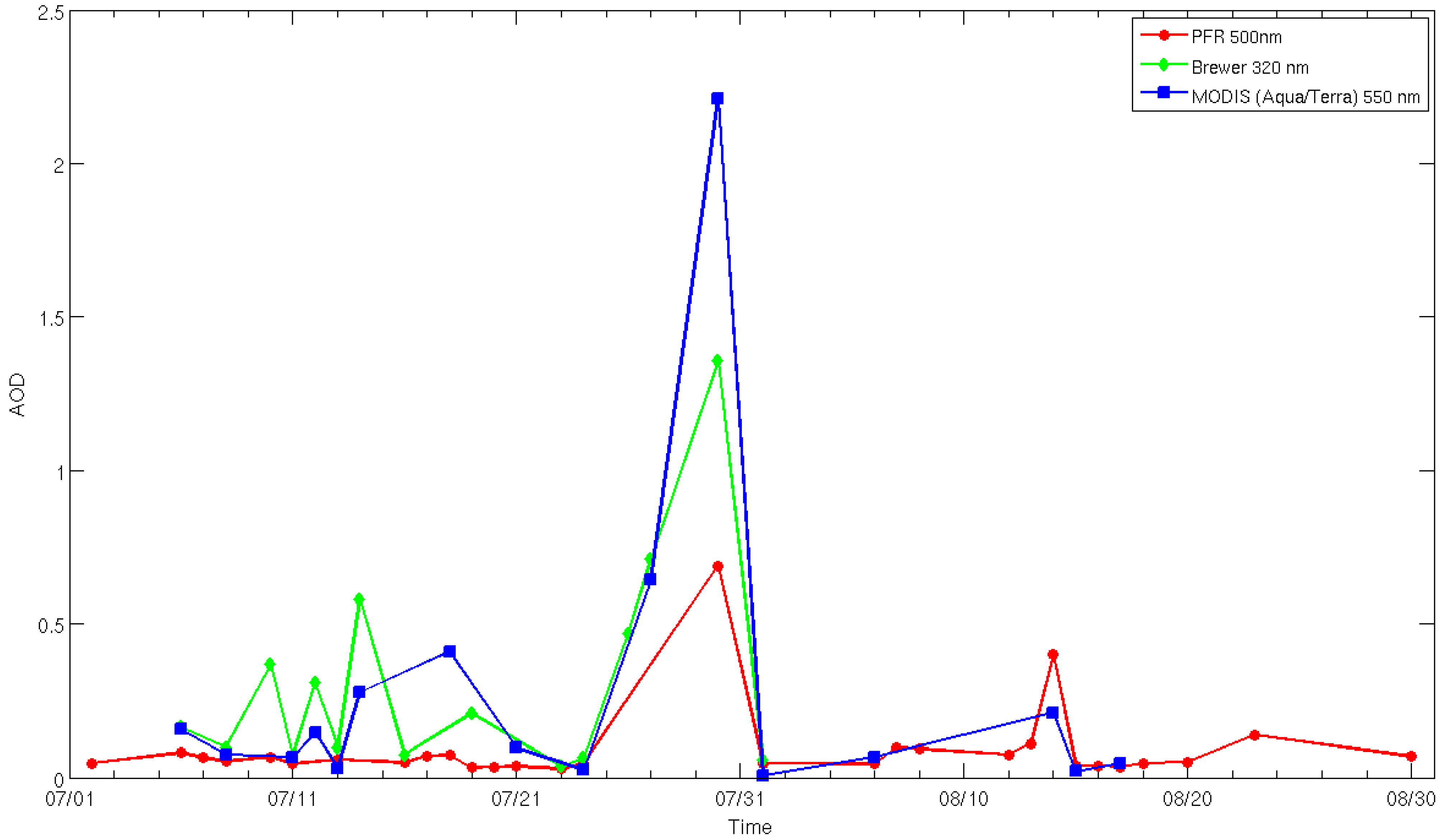
The daily averaged optical thickness of aerosols increased fourfold, while MODIS AOD was as high as 4.5 for the thickest part of the plume. Cloud screening algorithms may classify thick smoke plumes as clouds.
(2)
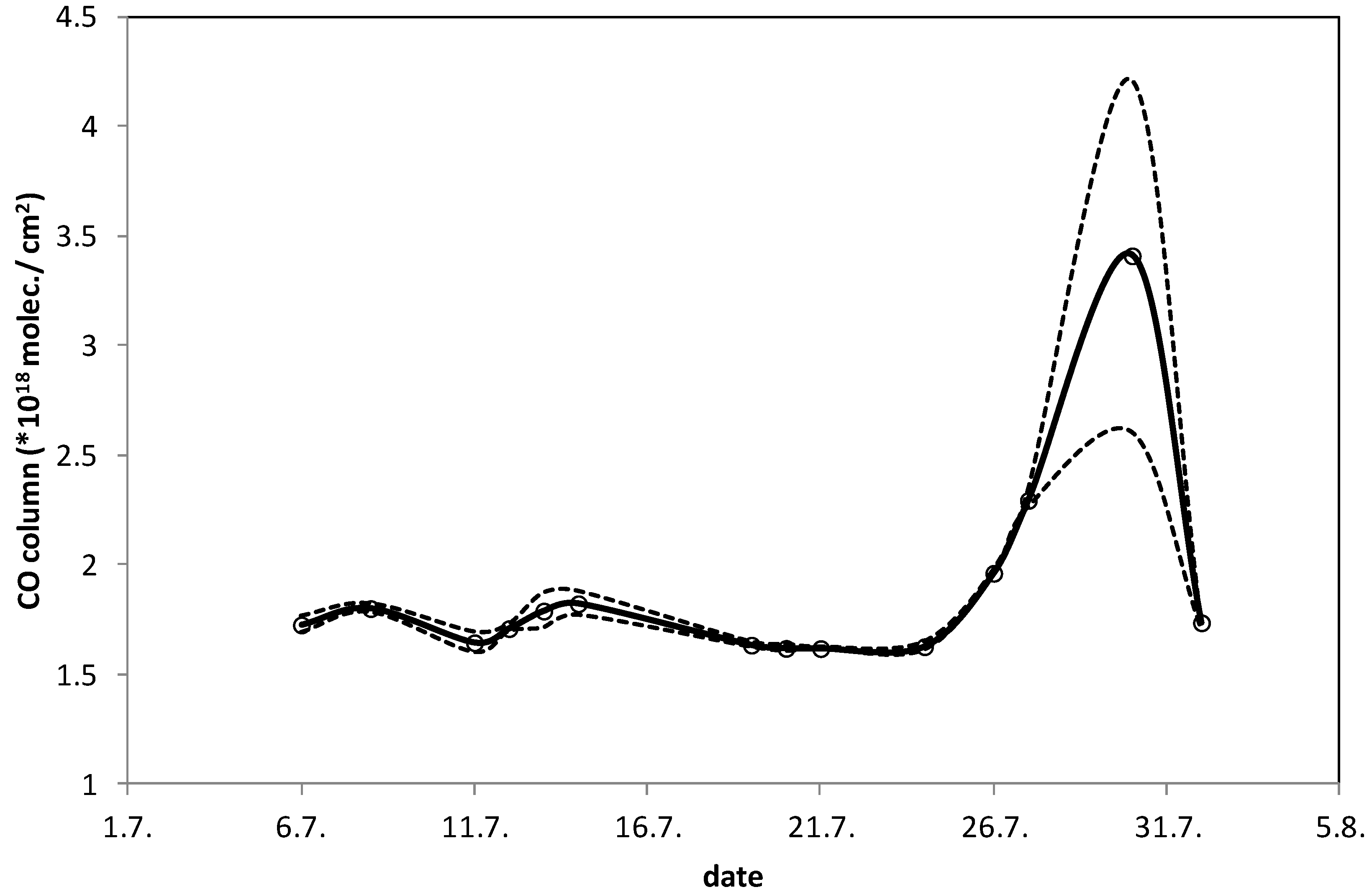
CO column abundance increased by 100%. According to the FTS measurements, the peak column abundance on 30 July was 5.32 × 10¹⁸ molecules/cm2.
(3)
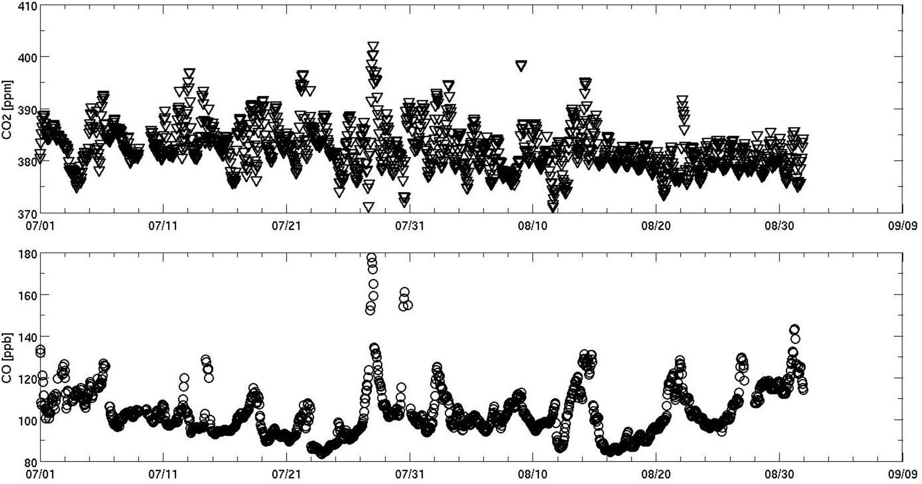
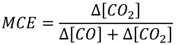
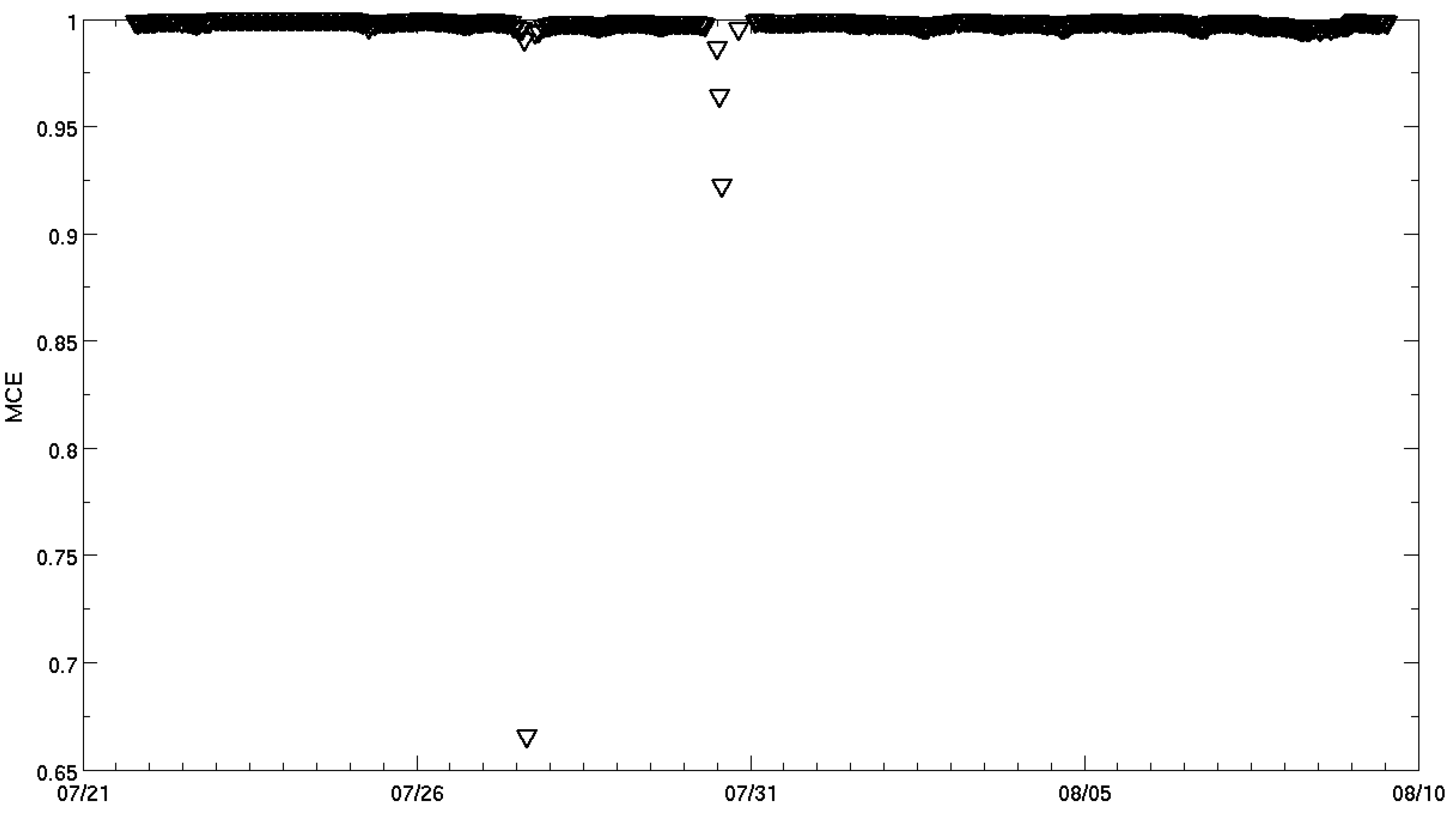
MCE values calculated from in situ CO and CO2 measurements indicated that the smoke plumes originated from flaming combustion (30 July) and smoldering peat combustion (27 July).
(4)
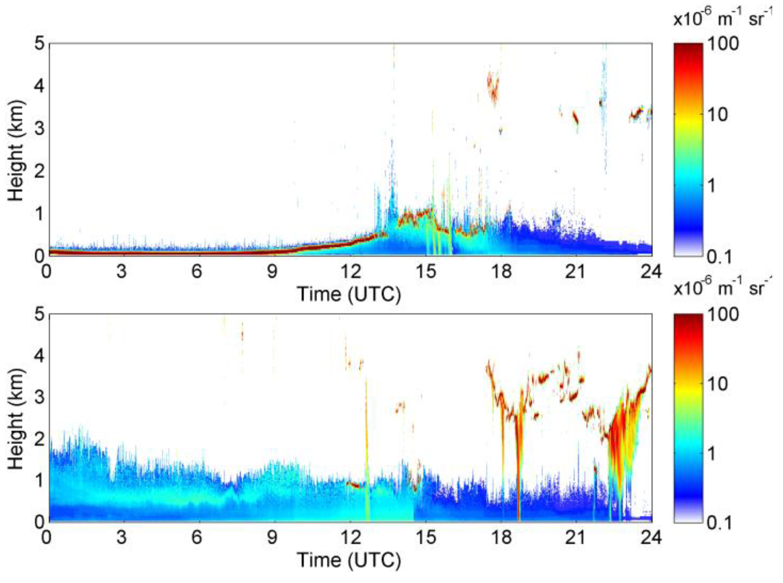
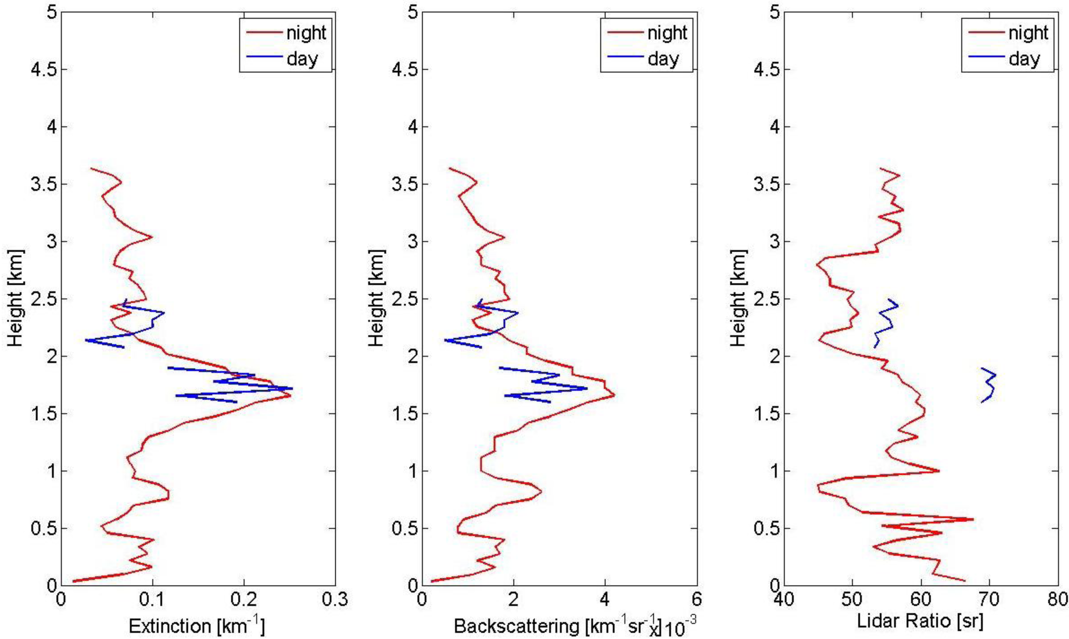
CALIOP and ceilometer measurements demonstrated that the smoke plume was located close to the surface, below 3 km, and the plume was not homogeneously mixed.
(5)
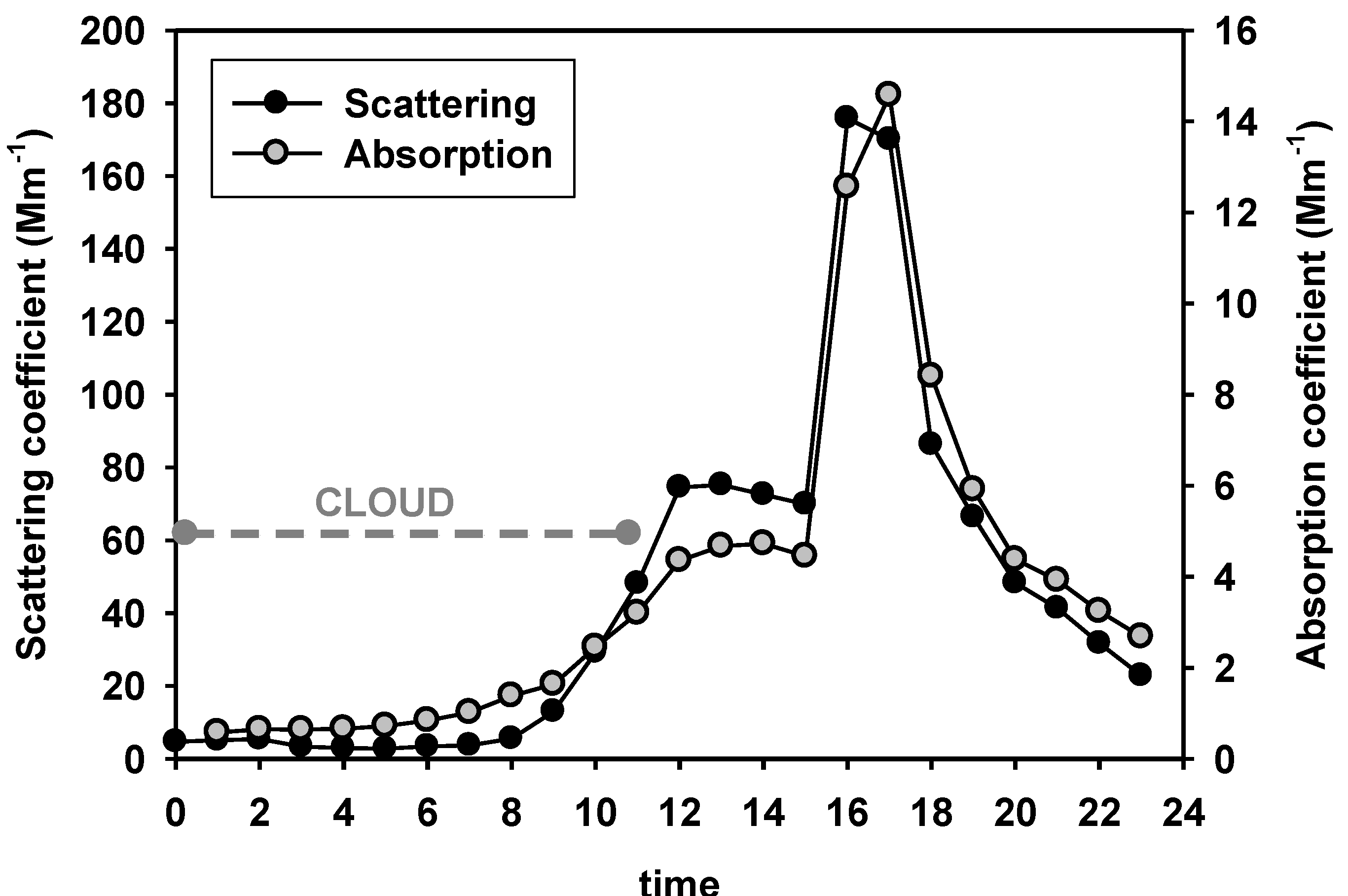
The scattering and absorption coefficients were almost 20 times larger in the smoke plume than in typical conditions.
(6)
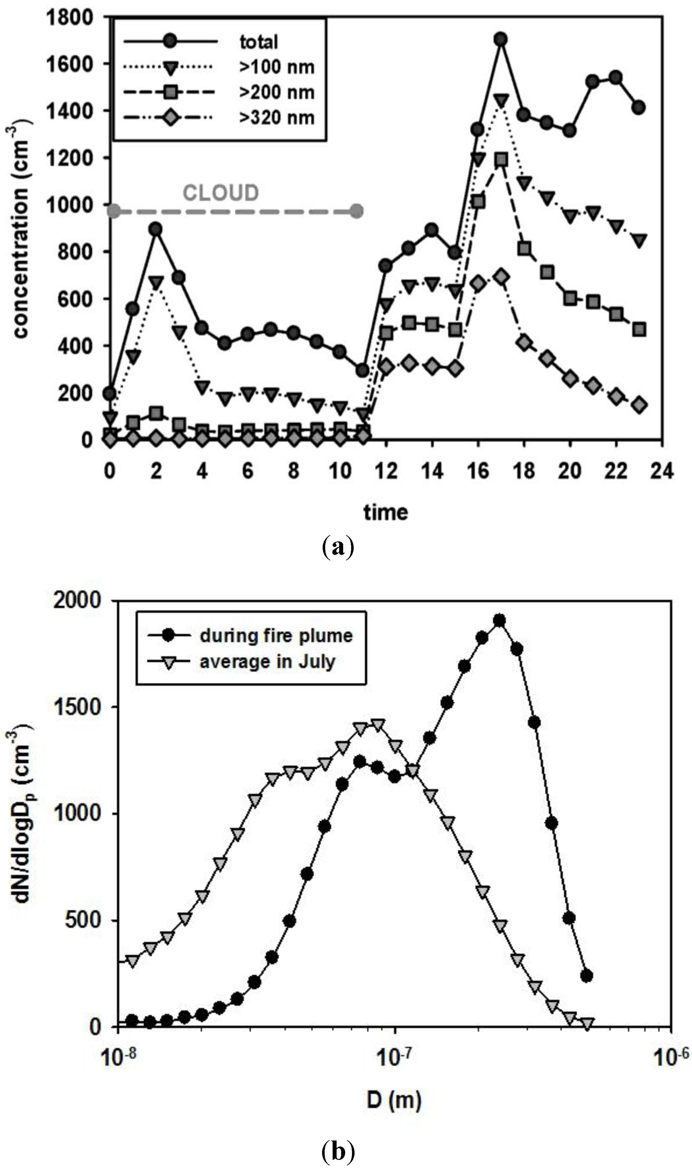
The total concentration of the aerosols did not change much. However, the number of particles larger than 320 nm increased 14-fold.
(7)
During the transport of the plume from eastern to northern Finland, the scattering coefficient, black carbon concentration, and total number concentration decreased 0.5%/h, 1.5%/h and 2.0%/h, respectively.

Acknowledgments

We acknowledge the MODIS, AIRS, CALIOP mission scientists and associated NASA personnel for the production of the data used in this research. CALIOP data were obtained from the NASA Langley Research Center Atmospheric Science Data Center. We also thank Janne Hakkarainen for the help with MODIS FRP data, Ewan O’Connor for providing the backscatter profiles from ceilometers data, Pauli Heikkinen for the help with the FTS data, Juha Hatakka for providing the trace gas information from Pallas, and Harri Portin for providing the in situ data from Kuopio.

References

  1. Barriopedro, D.; Fischer, E.M.; Luterbacher, J.; Trigo, R.M.; Garcia-Herrera, R. The hot summer of 2010: Redrawing the temperature record map of Europe. Science 2011, 332, 220–224. [Google Scholar] [CrossRef]
  2. Witte, J.C.; Douglass, A.R.; da Silva, A.; Torres, O.; Levy, R.; Duncan, B.N. NASA A-Train and Terra observations of the 2010 Russian wildfires. Atmos. Chem. Phys. 2011, 11, 9287–9301. [Google Scholar] [CrossRef]
  3. Mei, L.; Xue, Y.; de Leeuw, G.; Guang, J.; Wang, Y.; Li, Y.; Xu, H.; Yang, L.; Hou, T.; He, X.; et al. Integration of remote sensing data and surface observations to estimate the impact of the Russian wildfires over Europe and Asia during August 2010. Biogeosciences 2011, 8, 3771–3791. [Google Scholar]
  4. Yurganov, L.N.; Rakitin, V.; Dzhola, A.; August, T.; Fokeeva, E.; George, M.; Gorchakov, G.; Grechko, E.; Hannon, S.; Karpov, A.; et al. Satellite- and ground-based CO total column observations over 2010 Russian fires: Accuracy of top-down estimates based on thermal IR satellite data. Atmos. Chem. Phys. 2011, 11, 7925–7942. [Google Scholar] [CrossRef] [Green Version]
  5. van Donkelaar, A.; Martin, R.V.; Levy, R.; DaSilva, A.M.; Krzyzanowski, M.; Chubarova, N.E.; Semutnikova, E.; Cohen, A.J. Satellite-based estimates of ground-level fine particulate matter during extreme events: A case study of the Moscow fires in 2010. Atmos. Env. 2011, 45, 6225–6232. [Google Scholar]
  6. Konovalov, I.B.; Beekmann, M.; Kuznetsova, I.N.; Yurova, A.; Zvyagintsev, A.M. Atmospheric impacts of the 2010 Russian wildfires: Integrating modelling and measurements of an extreme air pollution episode in the Moscow region. Atmos. Chem. Phys. 2011, 11, 10031–10056. [Google Scholar]
  7. Warneke, C.; Froyd, K.D.; Brioude, J.; Bahreini, R.; Brock, C.A.; Cozic, J.; de Gouw, J.A.; Fahey, D.W.; Ferrare, R.; Holloway, J.S.; et al. An important contribution to springtime Arctic aerosol from biomass burning in Russia. Geophys. Res. Lett. 2010, 37, L01801. [Google Scholar]
  8. Barnaba, F.; Angelini, F.; Curci, G.; Gobbi, G.P. An important fingerprint of wildfires on the European aerosol load. Atmos. Chem. Phys. 2011, 11, 10487–10501. [Google Scholar] [CrossRef]
  9. Portin, H.J.; Mielonen, T.; Leskinen, A.; Arola, A.; Pärjälä, E.; Romakkaniemi, S.; Laaksonen, A.; Lehtinen, K.E.J.; Komppula, M. Biomass burning aerosols observed in Eastern Finland during the Russian wildfires in summer 2010—Part 1: In-situ aerosol characterization. Atmos. Environ. 2011, 45, 269–278. [Google Scholar]
  10. Mielonen, T.; Portin, H.J.; Komppula, M.; Leskinen, A.; Tamminen, J.; Ialongo, I.; Hakkarainen, J.; Lehtinen, K.E.J.; Arola, A. Biomass burning aerosols observed in Eastern Finland during the Russian wildfires in summer 2010—Part 2: Remote sensing. Atmos. Environ. 2011, 45, 279–287. [Google Scholar]
  11. Stohl, A.; Berg, T.; Burkhart, J.F.; Fjæraa, A.M.; Forster, C.; Herber, A.; Hov, Ø.; Lunder, C.; McMillan, W.W.; Oltmans, S.; et al. Arctic smoke—Record high air pollution levels in the European Arctic due to agricultural fires in Eastern Europe in spring 2006. Atmos. Chem. Phys. 2007, 7, 511–534. [Google Scholar] [CrossRef]
  12. Wehrli, C. Calibrations of filter radiometers for determination of atmospheric optical depth. Metrologia 2000, 37, 419–422. [Google Scholar] [CrossRef]
  13. Kim, S.-W.; Yoon, S.-C.; Dutton, E.G.; Kim, J.; Wehrli, C.; Holben, B.N. Global surface-based sun photometer network for long-term observations of column aerosol optical properties: Intercomparison of aerosol optical depth. Aerosol Sci. Tech. 2008, 42, 1–9. [Google Scholar] [CrossRef]
  14. Carlund, T.; Landelius, T.; Josefsson, W. Comparison and uncertainty of aerosol optical depth estimates derived from spectral and broadband measurements. J. Appl. Meteorol. 2003, 42, 1598–1610. [Google Scholar] [CrossRef]
  15. Smirnov, A.; Holben, B.N.; Eck, T.F.; Dubovik, O.; Slutsker, I. Cloud-screening and quality control algorithms for AERONET database. Remote. Sens. Environ. 2000, 73, 337–349. [Google Scholar] [CrossRef]
  16. International Ozone Services Inc. (IOS). 2012. Available online: http://www.io3.ca (accessed on 30 October 2012).
  17. de La Casinière, A.; Cachorro, V.; Smolskaia, I.; Lenoble, J.; Sorribas, M.; Houet, M.; Massot, O.; Antón, M.; Vilaplana, J.M. Comparative measurements of total ozone amount and aerosol optical depth during a campaign at El Arenosillo, Huelva, Spain. Ann. Geophys. 2005, 23, 3399–3406. [Google Scholar] [CrossRef]
  18. Marenco, F.; Santacesaria, V.; Bais, A.F.; Balis, D.; di Sarra, A.; Papayannis, A.; Zerefos, C. Optical properties of tropospheric aerosols determined by lidar and spectrophotometric measurements (photochemical activity and solar ultraviolet radiation campaign). Appl. Opt. 1997, 36, 6875–6886. [Google Scholar] [CrossRef]
  19. Carvalho, F.; Henriques, D. Use of Brewer ozone spectrophotometer for aerosol optical depth measurements on ultraviolet region. Adv. Space Res. 2000, 25, 997–1006. [Google Scholar] [CrossRef]
  20. Cheymol, A.; de Backer, H. Retrieval of aerosol optical depth in the UV-B at Uccle from Brewer ozone measurements over a long time period 1984-2002. J. Geophys. Res. 2003, 108((D24)), 4800. [Google Scholar] [CrossRef]
  21. Kazadzis, S.; Bais, A.; Kouremeti, N.; Gerasopoulos, E.; Garane, K.; Blumthaler, M.; Schallhart, B.; Cede, A. Direct spectral measurements with a Brewer spectroradiometer: Absolute calibration and aerosol optical depth retrieval. Appl. Opt. 2005, 44, 1691–1690. [Google Scholar] [CrossRef]
  22. Gröbner, J.; Meleti, C. Aerosol optical depth in the UVB and visible wavelength from Brewer spectrophotometer direct irradiance measurements: 1991-2002. J. Geophys. Res. 2004, 109, D09202. [Google Scholar] [CrossRef]
  23. Cheymol, A.; de Backer, H.; Josefsson, W.; Stuebi, R. Comparison and validation of the aerosol optical depth obtained with the Langley plot method in the UV-B from Brewer Ozone Spectrophotometer measurements. J. Geophys. Res. 2006, 111, D16202. [Google Scholar] [CrossRef]
  24. Cheymol, A.; Gonzalez Sotelino, L.; Lam, K.S.; Kim, J.; Fioletov, V.; Siani, A.M.; de Backer, H. Intercomparison of Aerosol Optical Depth from Brewer Ozone spectrophotometers and CIMEL sunphotometers measurements. Atmos. Chem. Phys. 2009, 9, 733–741. [Google Scholar] [CrossRef]
  25. Rinsland, C.P.; Mahieu, E.; Zander, R.; Jones, N.B.; Chipperfield, M.P.; Goldman, A.; Anderson, J.; Russell, J.M., III.; Demoulin, P.; Notholt, J.; et al. Long-term trends of inorganic chlorine from ground-based infrared solar spectra: Past increases and evidence for stabilization. J. Geophys. Res. 2003, 108, 4252. [Google Scholar] [CrossRef]
  26. Vigouroux, C.; de Mazière, M.; Demoulin, P.; Servais, C.; Hase, F.; Blumenstock, T.; Kramer, I.; Schneider, M.; Mellqvist, J.; Strandberg, A.; et al. Evaluation of tropospheric and stratospheric ozone trends over Western Europe from ground-based FTIR network observations. Atmos. Chem. Phys. 2008, 8, 6865–6886. [Google Scholar] [CrossRef]
  27. Wunch, D.; Toon, G.C.; Blavier, J.-F.L.; Washenfelder, A.; Notholt, J.; Connor, B.J.; Griffith, D.W.T.; Sherlock, V.; Wennberg, P.O. The total carbon column observing network. Phil. Trans. R. Soc. A 2011, 369, 2087–2112. [Google Scholar] [CrossRef]
  28. Salomonson, V.V.; Barnes, W.L.; Maymon, P.W.; Montgomery, H.E.; Ostrow, H. MODIS, advanced facility instrument for studies of the Earth as a system. IEEE T. Geosci. Remote Sens. 1989, 27, 145–153. [Google Scholar] [CrossRef]
  29. Levy, R.C.; Remer, L.A.; Mattoo, S.; Vermote, E.F.; Kaufman, Y.J. Second-generation operational algorithm: Retrieval of aerosol properties over land from inversion of Moderate Resolution Imaging Spectroradiometer spectral reflectance. J. Geophys. Res. 2007, 112, D13211. [Google Scholar] [CrossRef]
  30. Levy, R.C.; Remer, L.A.; Kleidman, R.G.; Mattoo, S.; Ichoku, C.; Kahn, R.; Eck, T.F. Global evaluation of the Collection 5 MODIS dark-target aerosol products over land. Atmos. Chem. Phys. 2010, 10, 10399–10420. [Google Scholar] [Green Version]
  31. Goddard Space Flight Center, Level 1 and Atmosphere Archive and Distribution System (LAADS Web). 2012. Available online: http://ladsweb.nascom.nasa.gov/data/search.html (accessed on 30 October 2012).
  32. Acker, J.G.; Leptoukh, G. Online analysis enhances use of NASA earth science data. Eos. Trans. AGU 2007, 88, 14–17. [Google Scholar] [CrossRef]
  33. Davies, D.K.; Ilavajhala, S.; Wong, M.M.; Justice, C.O. Fire information for resource management system: Archiving and distributing MODIS active fire data. IEEE Trans. Geosci. Remote Sens. 2009, 47, 72–79. [Google Scholar] [CrossRef]
  34. Aumann, H.H.; Chahine, M.T.; Gautier, C.; Goldberg, M.D.; Kalnay, E.; McMillin, L.M.; Revercomb, H.; Revercomb, P.W.; Revercomb, W.L.; Revercomb, D.H.; et al. AIRS/AMSU/HSB on the Aqua mission: Design, science objectives, data products, and processing systems. IEEE T. Geosci. Remote 2003, 41, 253–264. [Google Scholar] [CrossRef]
  35. Chahine, M.T.; Pagano, T.S.; Aumann, H.H.; Atlas, R.; Barnet, C.; Blaisdell, J.; Chen, L.; Divakarla, M.; Fetzer, E.J. AIRS: Improving weather forecasting and providing new data on greenhouse gases. Bull. Am. Meteor. Soc. 2006, 87, 911–926. [Google Scholar] [CrossRef]
  36. NASA, Giovanni, AIRS Online Visualization and Analysis. 2012. Available online: http://gdata.1.sci.gsfc.nasa.gov/daac-bin/G3/gui.cgi?instance_id=AIRS_Level3Daily (accessed on 30 October 2012).
  37. Winker, D.M.; Pelon, J.; McCormick, M.P. The CALIPSO mission: Spaceborne lidar for observation of aerosols and clouds. Proc. SPIE 2003, 4893, 1–11. [Google Scholar]
  38. Vaughan, M.; Young, S.; Winker, D.; Powell, K.; Omar, A.; Liu, Z.; Hu, Y.; Hostetler, C. Fully automated analysis of space-based lidar data: An overview of the CALIPSO retrieval algorithms and data products. Proc. SPIE 2004, 5575, 16–30. [Google Scholar]
  39. Winker, D.M.; Hunt, W.H.; McGill, M.J. Initial performance assessment of CALIOP. Geophys. Res. Lett. 2007, 34, L19803. [Google Scholar] [CrossRef]
  40. Vaisala Oyj, Ceilometer CT25K: User’s Guide; Vaisala Oyj: Vantaa, Finland, 2002.
  41. Emeis, S.; Münkel, C.; Vogt, S.; Müller, W.J.; Schäfer, K. Atmospheric boundary-layer structure from simultaneous SODAR, RASS and ceilometer measurements. Atmos. Environ. 2004, 38, 273–286. [Google Scholar] [CrossRef]
  42. Eresmaa, N.; Karppinen, A.; Joffre, S.M.; Räsänen, J.; Talvitie, H. Mixing height determination by ceilometers. Atmos. Chem. Phys. 2006, 6, 1485–1493. [Google Scholar] [CrossRef]
  43. Hatakka, J.; Aalto, T.; Aaltonen, V.; Aurela, M.; Hakola, H.; Komppula, M.; Laurila, T.; Lihavainen, H.; Paatero, J.; Salminen, K.; Viisanen, Y. Overview of the atmospheric research activities and results at Pallas GAW station. Boreal Env. Res. 2003, 8, 365–384. [Google Scholar]
  44. Aaltonen, V.; Lihavainen, H.; Kerminen, V.-M.; Komppula, M.; Hatakka, J.; Eneroth, K.; Kulmala, M.; Viisanen, Y. Measurements of optical properties of atmospheric aerosols in Northern Finland. Atmos. Chem. Phys. 2006, 6, 1155–1164. [Google Scholar] [CrossRef]
  45. Hyvärinen, A.-P.; Kolmonen, P.; Kerminen, V.-M.; Virkkula, A.; Leskinen, A.; Komppula, M.; Hatakka, J.; Burkhart, J.; Stohl, A.; Aalto, P.; et al. Aerosol black carbon at five background measurement sites over Finland, a gateway to the Arctic. Atmos. Env. 2011, 45, 4042–4050. [Google Scholar]
  46. Komppula, M.; Lihavainen, H.; Hatakka, J.; Paatero, J.; Aalto, P.; Kulmala, M.; Viisanen, Y. Observations of new particle formation and size distributions at two different heights and surroundings in subarctic area in northern Finland. J. Geophys. Res. 2003, 108, 4295. [Google Scholar] [CrossRef]
  47. Ward, D.E.; Radke, L.F. Fire in the Environment: The Ecological, Atmospheric, and Climatic Importance of Vegetation Fires; Dahlem Workshop Reports; Environmental Sciences Research Report 13; Crutzen, P.J., Goldammer, J.G., Eds.; John Wiley & Sons: Chischester, UK, 1993; pp. 53–76. [Google Scholar]
  48. Reid, J.S.; Koppmann, R.; Eck, T.F.; Eleuterio, D.P. A review of biomass burning emissions part II: Intensive physical properties of biomass burning particles. Atmos. Chem. Phys. 2005, 5, 799–825. [Google Scholar] [CrossRef]
  49. Draxler, R.R.; Hess, G.D. Description of the HYSPLIT_4 Modeling System. NOAA Technical Memorandum ERL ARL-224; NOAA Air Resources Laboratory: Silver Spring, MD, USA, 1997; p. 24. [Google Scholar]
  50. Draxler, R.R.; Rolph, G.D. HYSPLIT—HYbrid Single-Particle Lagrangian Integrated Trajectory Model. Available online: http://ready.arl.noaa.gov/HYSPLIT.php (accessed on 30 October 2012).
  51. Rolph, G.D. Real-time Environmental Applications and Display sYstem (READY). Available online: http://ready.arl.noaa.gov (accessed on 30 October 2012).
  52. Iinuma, Y.; Brüggemann, E.; Gnauk, T.; Müller, K.; Andreae, M.O.; Helas, G.; Parmar, R.; Herrmann, H. Source characterization of biomass burning particles: The combustion of selected European conifers, African hardwood, savanna grass, and German and Indonesian peat. J. Geophys. Res. 2007, 112. [Google Scholar] [CrossRef]
  53. Reid, J.S.; Eck, T.F.; Christopher, S.A.; Koppmann, R.; Dubovik, O.; Eleuterio, D.P.; Holben, B.N.; Reid, E.A.; Zhang, J. A review of biomass burning emissions part III: Intensive optical properties of biomass burning particles. Atmos. Chem. Phys. 2005, 5, 827–849. [Google Scholar] [CrossRef]
  54. Komppula, M.; Lihavainen, H.; Kerminen, V.; Kulmala, M.; Viisanen, Y. Measurements of cloud droplet activation of aerosol particles at a clean subarctic background site. J. Geophys. Res. 2005, 110, D06204. [Google Scholar] [CrossRef]

