Low-Frequency Rotation of Surface Winds over Canada

Abstract

Hourly surface observations from the Canadian Weather Energy and Engineering Dataset were analyzed with respect to long-term wind direction drift or rotation. Most of the Canadian landmass, including the High Arctic, exhibits a spatially consistent and remarkably steady anticyclonic rotation of wind direction. The period of anticyclonic rotation recorded at 144 out of 149 Canadian meteostations directly correlated with latitude and ranged from 7 days at Medicine Hat (50°N, 110°W) to 25 days at Resolute (75°N, 95°W). Only five locations in the vicinity of the Rocky Mountains and Pacific Coast were found to obey a “negative” (i.e., cyclonic) rotation. The observed anticyclonic rotation appears to be a deterministic, virtually ubiquitous, and highly persistent feature of continental surface wind. These findings are directly applicable to probabilistic assessments of airborne pollutants.

1. Introduction

There is an increasing demand for high accuracy prediction of low-level winds in applications such as wind power, wildfire management and air quality assessments. The latter can concern terrorist threats (where the location of source is frequently unknown), emergency planning, probabilistic safety assessments pertaining to design-based accidents and licensing submissions pertaining to routine industrial releases. One of the most important parameters required by these applications is the speed and direction of the wind, which is rarely known both at the source and at the receptor. Characteristics of the wind for a specific location can be assimilated from point measurement sites and (or) dynamically interpolated using a mesoscale numerical model.

The need for improving the accuracy of mesoscale models is on-going, and increasing the model resolution (by diminishing the grid-cell size) was generally associated with a gain in predictions accuracy, however there is a limit to the effectiveness of this approach [1]. For example, in the case of the Weather Research and Forecasting model and Mesoscale Model Version 5 (MM5) the best scale appeared to be limited by a 1 km grid spacing, because no improvement in the modeling of near-surface wind speed and direction was established at the sub-kilometer scale [2]. Further difficulties are caused by the models generally poor ability to represent wind speed, and especially wind direction, in periods of transition from a convective and unstable boundary layer in the daytime to a stable boundary layer at night [3,4]. In addition, numerical mesoscale models are particularly poor in predicting sudden, large directional shifts in noctural winds [5]. In contrast to the generally acceptable accuracy of predictions of wind speed [6], performance is poorer for wind directions, where anomalies can exceed 100° in the stable boundary layer [5].

As many air quality applications (e.g., safety and licensing of industrial sources of pollutants) are based on probabilistic assessments of atmospheric transport and dispersion, it is important to know whether there is an accumulation of a significant bias, or whether these anomalies largely cancel out when the long term record of modeled wind is deployed. This is a motivation for our work which focuses on the in-situ quantification of deterministic large-scale spatio-temporal patterns in the evolution of wind and subsequent quantification of the associated wind variability.

Deterministic in-situ quantification of wind and particularly its low-frequency variability (LFV) immediately beyond the synoptic scale (7–30 days) has been sought, but as yet remains elusive. Indirect support for the existence of beyond-synoptic LFV at the surface comes from the observations of LFV aloft in the mid atmosphere. For example, Hamilton [7] reported 5- and 16-day waves, and Luo and colleagues [8,9] reported waves over Saskatchewan with 12- to 24-day periods.

Further support for atmospheric LFV is provided by periodicity observed in global Reanalyses data, particularly in that of ECMWF ERA-15 and NCEP-DOE [10], ECMWF ERA-40 [11,12], and NCEP-NCAR [13]. Especially relevant to our study is that the period of mid-atmospheric LFV in the northern hemisphere (NH) ranged from 2 to 20 days [12].

Our study was focused on the analysis of continental surface wind, particularly its directional rotation. Historical records of wind rotation go back to observations of anticyclonic rotation of wind that have been reported in regions subjected to diurnally oscillating forces of land-sea breezes [14,15,16,17,18]. According to Kuo, Polvani [19] and Shipton [20], farther inland, away from diurnal sea breeze, the rotational nature of wind is expected to present itself in low-frequency rotation in the same anticyclonic direction. This rotation (i.e., the net anticyclonic imbalance of cyclonic and anticyclonic events, also termed “cyclonic-anticyclonic asymmetry”) has been demonstrated in laboratory experiments and numerical simulations [19,20]. The Coriolis force is usually attributed as being one of the causes of this anticyclonic asymmetry.

It is important to note that, although anticyclonic rotation is expected to dominate, cyclonic rotations are nevertheless frequently reported in the NH at as many as nearly half of the analyzed stations [21,22,23]. These negative cyclonic rotations are mainly confined to narrow regions adjacent to the coast (i.e., Pacific Coast of North America, Mediterranean and Japan) and to those regions influenced by steep large-scale orography.

The objective of our study is to present observational evidence for the existence of LFV in surface winds, to quantify surface winds’ LFV (frequency and direction of rotation) and to show that observed LFV of wind is spatially consistent over the continent. In addition, we show that regions influenced by the coast and by large-scale orography provide the exception to the general rule of “positive” (anticyclonic) and spatially consistent rotation.

The paper is organized as follows. Section 2 outlines the methodology of the study primarily based on the reconstruction of a continuous record of rotation of vane anemometer from the traditional discontinuous compass-based record. Section 2 also outlines the analysis of the reconstructed point time series performed using the regression and rotary spectra analyses, followed by the spatial analysis of the pattern of trends encountered at different stations using the robust Kendall test for small datasets. Section 3 presents results pertaining to surface winds rotation (SWR), including the derivation of SWR stationarity on a multi-decadal scale and its latitudinal dependence. Section 4 is the discussion, and Section 5 provides the conclusions.

2. Methods

2.1. Datasets and Data Quality

Multi-decadal records of hourly observations of wind were obtained from a publicly available Canadian Weather Energy and Engineering Dataset (CWEEDS) representing the period from 1953 to 2003 [24]. All 235 CWEEDS stations were ranked according to the relative length of the maximum gap in each station’s annual record. The trade-off between the record quality and a representative continent-wide coverage was achieved with a sub-set of 149 stations, where the largest temporal data gap did not exceed 12%. On average 3% of the hourly data was missing.

The 149 stations selected comprised of 131 Weather-Bureau-Army-Navy (WBAN) stations and 18 other stations recently added to CWEEDS. Gap-filling methods for sporadic temporal omissions in the surface wind data for the 149 Canadian meteostations and for calms (where no actual wind direction was identified) were based on the work of Fernandes and colleagues [25]—small data gaps in wind direction were filled by interpolation and longer data gaps (outages, etc.) were taken from the similar period of the highest quality year on the record. The wind rose data documented for 1953 to 1980 in the Canadian Weather Atlas [26] was used for quality control, as it conveniently matched part of the time period covered by data from the selected CWEEDS stations.

2.2. Reconstruction of a Continuous Record of Wind Direction Drift

Full rotations completed by the vane anemometer are absent in the standard record of wind direction due to discontinuity when crossing the compass bearings from 360° to 0°. The traditional compass-based CWEEDS data was therefore reconstructed to accommodate directional continuity by adding 360° to the wind direction angle if the indication was that the wind direction passed through 360°/0°. For example, if five consecutive anticyclonic readings were 270°, 290°, 5°, 10°, and 30°, then this data was reconstituted as 270°, 290°, 365°, 370°, and 390°. Readings indicating a cyclonic rotation were treated in a similar fashion (i.e., 30°, 10°, 5°, 290°, and 270° could have been reconstituted as 750°, 730°, 725°, 650°, and 630°).

Therefore, reconstruction of full rotation counts at the 360°/0° crossing appears a generally straightforward task even when taking into account infrequent occurrences of large shifts in wind direction. Large wind shifts in the standard compass-based record of say +270° were substituted by the smaller and thus more likely shifts in the opposite direction, i.e., −90°, complemented by a full rotation count being added to the reconstructed record (in this case the count was −1 as 360° was subtracted from +270° and not added). Ambiguity as to whether the rotation was cyclonic or anticyclonic could, however, occur for two consecutive wind directions that had a difference angle approaching 180°, indicating a near reversal in direction. According to Mahrt [27], detailed reconstruction of wind direction change requires the comparison of winds averaged over various time window widths. In this study, for simplicity, a limiting threshold difference angle was used in the reconstruction of the wind direction data to reduce the ambiguity that is most pronounced for 180° changes. Instead of a 180° threshold, a more conservative threshold angle of 120° was employed to differentiate the directional shift from discontinuity and to calculate long-term direction drift, as this threshold angle results in a tolerable error of 9% in the rotation rate. In this way, only direction shifts of larger than 240° were interpreted as artifacts of the discontinuity crossings and were accommodated as an indication of the subsequent complete rotations (which were added as multiples of 360° to the traditional wind direction angle, so that a trend in the continuous record of historic wind direction angle was reconstructed). The reconstruction error of ±9% corresponds to missing counts of complete rotations that occur (in both directions of rotation) at discontinuities not distinguished among shifts in the range from 120° to 240°, which were all considered as simple shifts and thus were left intact.

In the present study, the trend in wind direction drift (specifically, the net anticyclonic drift) is termed SWR, instead of the more broadly defined term LFV. The long-term average of SWR was assigned a positive value if anticyclonic (i.e., clockwise in the NH) and a negative value if cyclonic (i.e., anticlockwise in the NH) [14,15].

2.3. Temporal Analysis of Point Surface Winds: SWR Drift

Wind direction drift (trend) was established and analyzed for all 149 selected CWEEDS stations. The degree of long-term stationarity of rotation was assessed by linear correlations of the continuous SWR record to time (i.e., to the linear trend). The robustness of the established SWR effect was assessed on the basis of wind rotary spectra analysis [28,29].

2.4. Zonal and Meridional Analysis of SWR

Spatial analysis consisted of investigating the zonal structure of SWR by assessing the correlation of SWR with longitude within the whole dataset and in moderately narrow (i.e., ~10°-wide) E-W transects. Meridional dependence was investigated by comparison of SWR with an analytical expression based on latitude rather than with the latitude per se. The analytical meridional structure of SWR (and SWR latitudinal dependence) was identified by least-squares fit to the SWR latitudinal distribution in a mid-continental (80°W–90°W) N-S transect. This mid-continental analytical latitudinal dependence was further evaluated in all other transects, using the Kendall non-parametric test [30,31] on correlation with each station’s average SWR. The whole dataset has also been evaluated using the Kendall test: the arbitrary Kendall-tau (dispersion threshold) divided the dataset into the core subset with clear latitudinal dependence and a subset of exceptions.

Figure 1. Standard record of wind direction (the upper panel, limited to the end of 2001) and the corresponding reconstruction of the continuous evolution of wind direction at North Bay Ontario, 46.37°N, 79.42°W during 1953–2001. The upper three plots represent wind direction in degrees versus day of the year (DOY). Due to the large temporal scalethe lowermost plot, represents complete rotations of wind versus years.

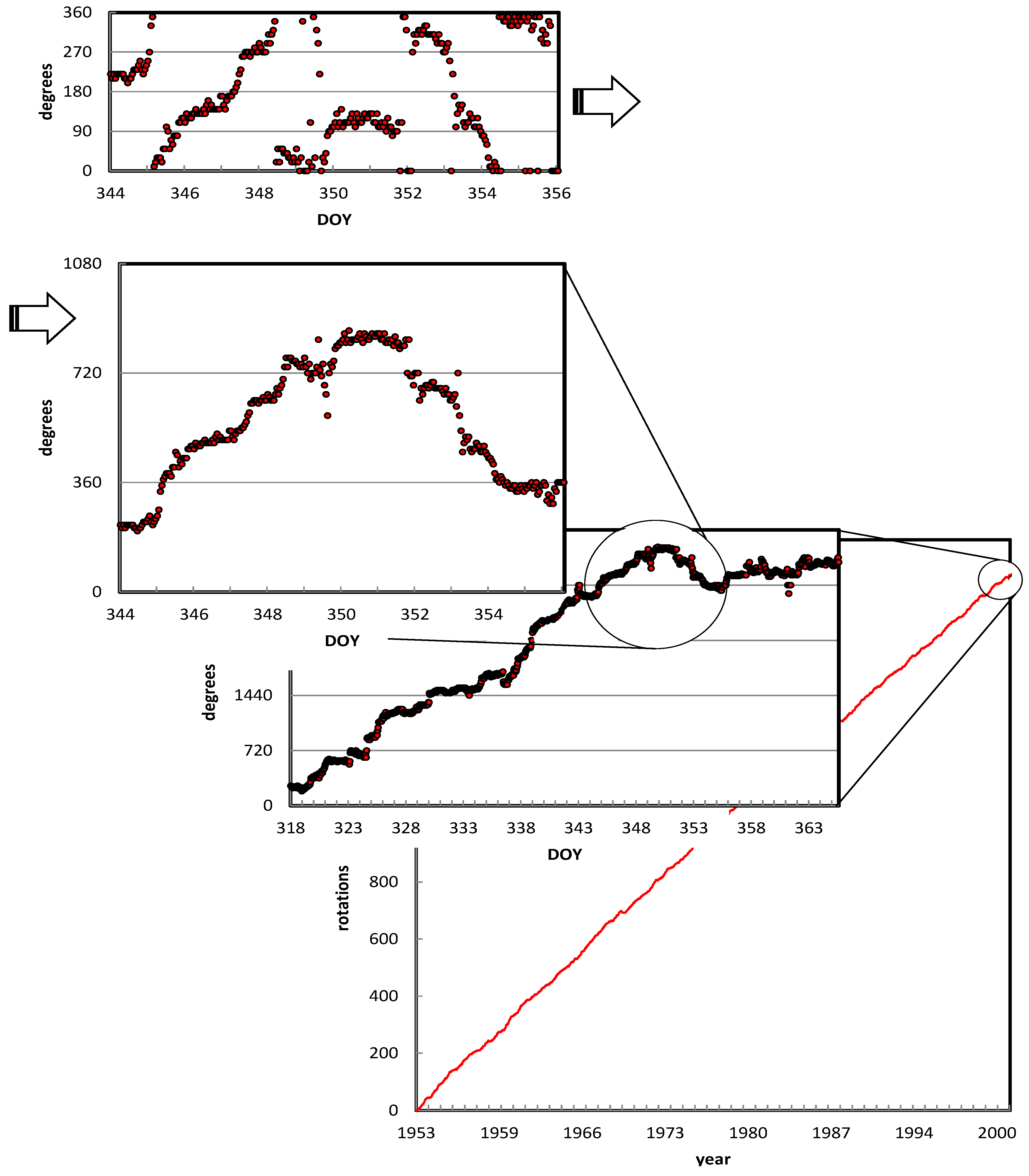
Figure 1. Standard record of wind direction (the upper panel, limited to the end of 2001) and the corresponding reconstruction of the continuous evolution of wind direction at North Bay Ontario, 46.37°N, 79.42°W during 1953–2001. The upper three plots represent wind direction in degrees versus day of the year (DOY). Due to the large temporal scalethe lowermost plot, represents complete rotations of wind versus years.

3. Results

3.1. Basic Asymmetry: Net Rotation of Surface Winds

The net anticyclonic drift, or SWR, subsequently represents the net asymmetry between cyclones and anticyclones. Observations of much longer than a month are required to clearly identify consistent anticyclonic SWR and to subsequently measure SWR frequency (Figure 1). The last five decades documented in CWEEDS (1953–2003) thus provide a convenient framework for identification of SWR and analysis of its frequency.

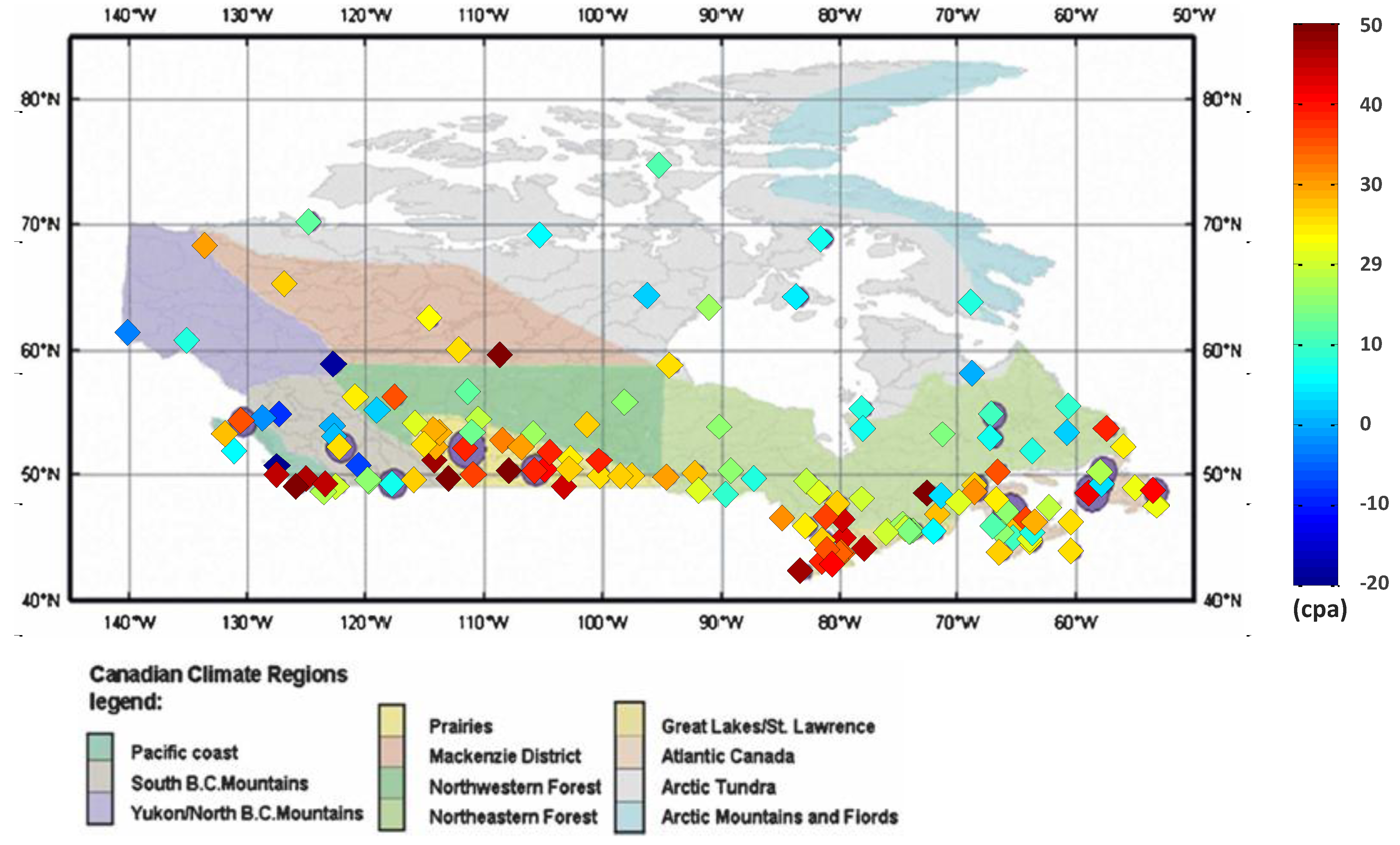
Most of the Canadian landmass (144 out of 149 meteostations), including the High Arctic, appears to be marked by anticyclonic SWR (Figure 2). The mean period of observed anticyclonic rotation ranged from 7 days (52 rotations, or cycles per annum, cpa) at Medicine Hat (50°N, 110°W) to 25 days (15 cpa) at Resolute (75°N, 95°W), in the latter case—well beyond the synoptic range.

Figure 2. Map of Canadian climate regions with mean SWR rates observed at 149 CWEEDS stations; marker’s color is mapped to SWR cycles per annum (cpa). Anticyclonic (clockwise) rotation is assigned a positive (+) sign, and cyclonic (anticlockwise) rotation is assigned a negative (–) sign.

Figure 2. Map of Canadian climate regions with mean SWR rates observed at 149 CWEEDS stations; marker’s color is mapped to SWR cycles per annum (cpa). Anticyclonic (clockwise) rotation is assigned a positive (+) sign, and cyclonic (anticlockwise) rotation is assigned a negative (–) sign.

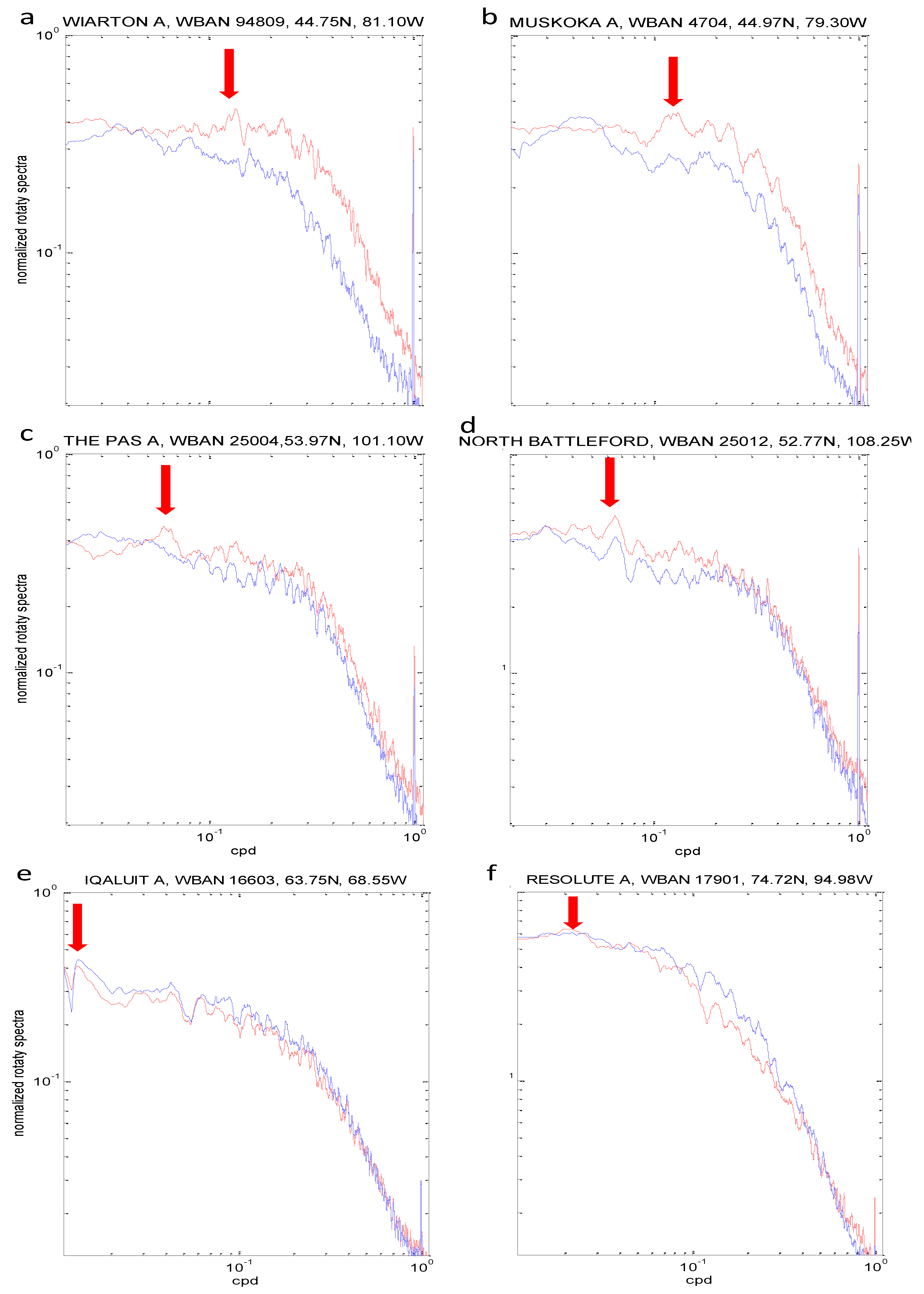
In addition to the analysis of the continuous SWR (completed by vane anemometer), the rotary spectra of wind were calculated at 15 random locations in order to assess the robustness of the observed SWR effect. The frequency corresponding to SWR was clearly seen in each analyzed case; this is illustrated in Figure 3 depicting 6 locations. The net anticyclonic rotation follows from generally larger magnitude of the corresponding clockwise rotational component. However, the unambiguous identification of the SWR frequency based solely on the rotary spectra would have been difficult.

Figure 3. Zoomed fragment of rotary wind spectra between known diurnal and seasonal oscillations at six Canadian Weather Energy and Engineering Dataset (CWEEDS) stations: (a) Wiarton, (b) Muskoka, (c) The Pas, (d) North Battleford, (e) Iqaluit, (f) Resolute. The red line is the clockwise anticyclonic component and the blue line is the counter-clockwise cyclonic component. The frequency of the net rotation of wind (SWR) is marked by a red arrow. The spectra are normalized by their respective standard deviations.

Figure 3. Zoomed fragment of rotary wind spectra between known diurnal and seasonal oscillations at six Canadian Weather Energy and Engineering Dataset (CWEEDS) stations: (a) Wiarton, (b) Muskoka, (c) The Pas, (d) North Battleford, (e) Iqaluit, (f) Resolute. The red line is the clockwise anticyclonic component and the blue line is the counter-clockwise cyclonic component. The frequency of the net rotation of wind (SWR) is marked by a red arrow. The spectra are normalized by their respective standard deviations.

3.2. Stationarity of SWR on a Decadal Scale

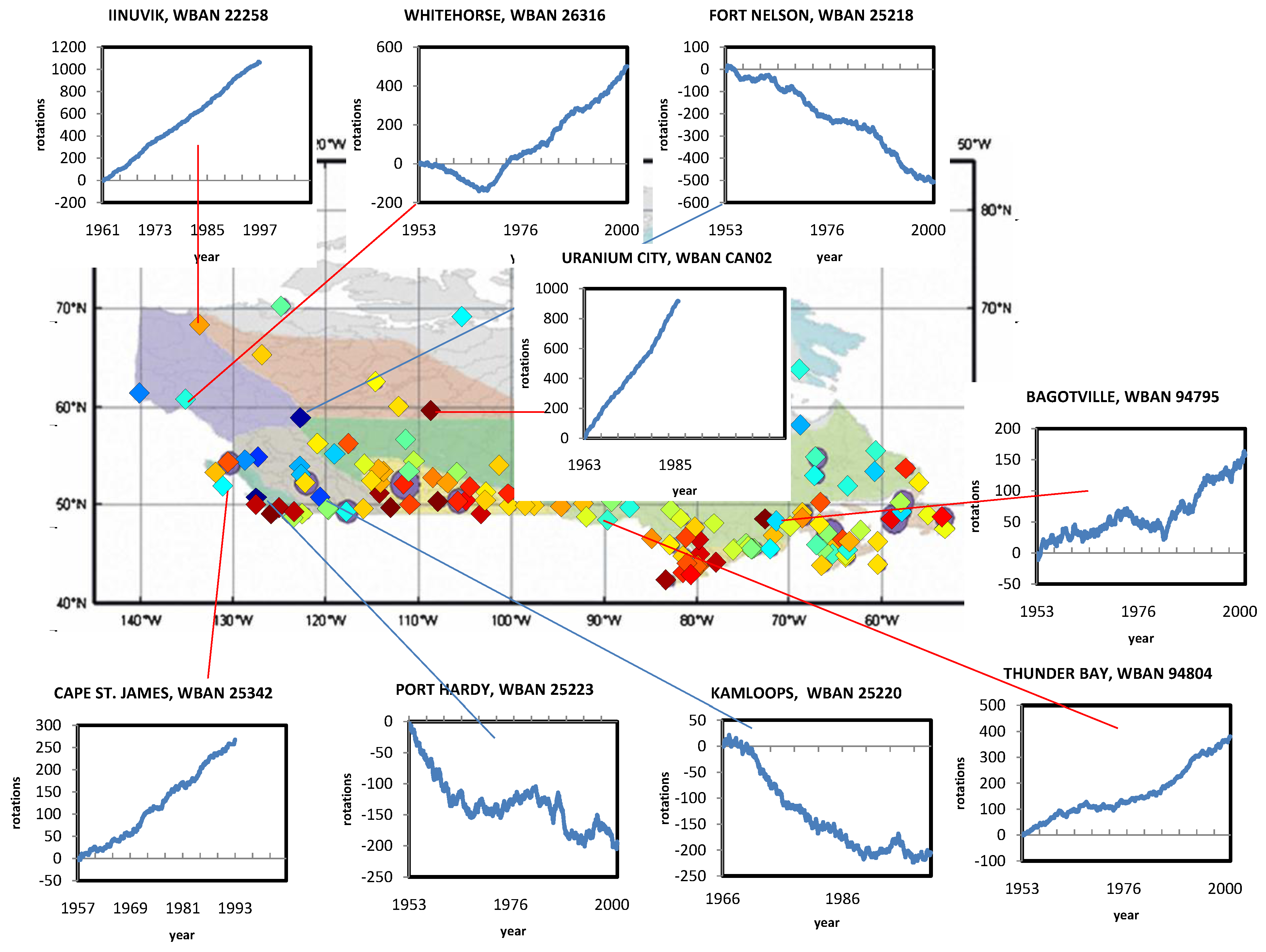
Most of the Canadian landmass, including the High Arctic, exhibits anticyclonic and steady SWR, which also appears directly correlated with latitude (as seen in Figure 4, Table 1 and explained in Section 3.3). Clear examples of SWR steadiness are provided in Figure 5, as shown by inserted plots for nine stations showing wind direction angle drift over several decades. Table 1 presents a test on steadiness of rotation, based on a linear least squares fit to constant rotation (i.e., to time).

Table 1. Test on stationarity and on latitudinal dependence of SWR performed in 9 N-S transects. The number of stations in each transect is n, the maximum tolerance for temporal trend significance in the transect is α_max, coefficient of determination in time is R², significance of fit to Equation (1) is Kendall α_K and goodness of fit to Equation (1) is Kendall-tauτ_K.

Transect Width	Province a	n	α max	R2	α Κ	τ Κ
52.8W–59.9W	NFL	9	0.05	0.97	-	-
60.0W–69.9W	NFL,NB,NS,PEI,QC,NWT	25	0.01	0.98	0.1	0.26
70.9W–79.9W	QC, SE-ON	26	0.1	0.81	0.05	0.33
80.0W–89.9W	NW-ON, NU	16	0.1	0.9	0.01	0.72
90.0W–99.9W	NW-ON, MAN, NU	10	0.01	0.99	0.05	0.57
100.0W–109.9W	MAN, SASK, NU, NWT	15	0.05	0.96	0.1	0.33
110.0W–119.9W	ALTA, NU, NWT	16	0.01	0.99	0.01	0.54
120.0W–129.9W	BC, YU, NWT	18	0.01	0.89	-	-
130.0W–140.0W	YU, NWT	6	0.05	0.96	-	-
Outliers b	BC (4), QC (2), YU (2)	8	0.01	0.94	-	-

^a Province abbreviations: ALTA: Alberta; BC: British Columbia; MAN: Manitoba; NB: New Brunswick; NFL: Newfoundland; NS: Nova Scotia; NW-ON: NW-Ontario; NWT: North West Territories; NU: Nunavut; PEI: Prince Edward Island; QC: Quebec; SASK: Saskatoon; SE-ON: SE-Ontario; YU: Yukon.

^b Set comprises of 5 stations with cyclonic SWR and 3 with intermittent and nonsteady SWR; the number of stations is presented in parentheses beside the province name.

Table 1. Test on stationarity and on latitudinal dependence of SWR performed in 9 N-S transects. The number of stations in each transect is n, the maximum tolerance for temporal trend significance in the transect is α_max, coefficient of determination in time is R², significance of fit to Equation (1) is Kendall α_K and goodness of fit to Equation (1) is Kendall-tauτ_K.

Transect Width	Province a	n	α max	R2	α Κ	τ Κ
52.8W–59.9W	NFL	9	0.05	0.97	-	-
60.0W–69.9W	NFL,NB,NS,PEI,QC,NWT	25	0.01	0.98	0.1	0.26
70.9W–79.9W	QC, SE-ON	26	0.1	0.81	0.05	0.33
80.0W–89.9W	NW-ON, NU	16	0.1	0.9	0.01	0.72
90.0W–99.9W	NW-ON, MAN, NU	10	0.01	0.99	0.05	0.57
100.0W–109.9W	MAN, SASK, NU, NWT	15	0.05	0.96	0.1	0.33
110.0W–119.9W	ALTA, NU, NWT	16	0.01	0.99	0.01	0.54
120.0W–129.9W	BC, YU, NWT	18	0.01	0.89	-	-
130.0W–140.0W	YU, NWT	6	0.05	0.96	-	-
Outliers b	BC (4), QC (2), YU (2)	8	0.01	0.94	-	-

^a Province abbreviations: ALTA: Alberta; BC: British Columbia; MAN: Manitoba; NB: New Brunswick; NFL: Newfoundland; NS: Nova Scotia; NW-ON: NW-Ontario; NWT: North West Territories; NU: Nunavut; PEI: Prince Edward Island; QC: Quebec; SASK: Saskatoon; SE-ON: SE-Ontario; YU: Yukon.

^b Set comprises of 5 stations with cyclonic SWR and 3 with intermittent and nonsteady SWR; the number of stations is presented in parentheses beside the province name.

In Table 1, eight stations, where negative cyclonic rotation occurs either permanently (at five stations in British Columbia and Yukon) or persistently over a year or longer (Whitehorse in Yukon, and Kuujuaq and Bagotville in Quebec), were set aside and grouped as “outliers”. For each N-S transect listed in Table 1, the significance level (α_max) of maximum tolerance of a linear relationship between each transect station’s SWR rate versus time was recorded.

Table 1 also provides the coefficient of determination (R²) of SWR with time for all stations in each transect. Dispersion is mostly attributed to seasonal SWR variability accompanied by a much smaller interannual variability. Long-term stationarity appears strong across Canada (including the set of 8 outliers) because the least squares fit to constant rotation is consistently significant at level α_max ≤ 0.1 (and mostly at level α ≤ 0.01), with dispersion characterized by R² ≥ 0.8.

3.3. Zonal and Meridional Structure of SWR

No significant association was found at the level of α ≤ 0.1 for SWR correlation with longitude, either for the continent-wide data set (n = 149) or within the 10°-wide E-W transects. Therefore, no zonal dependency in SWR was established.

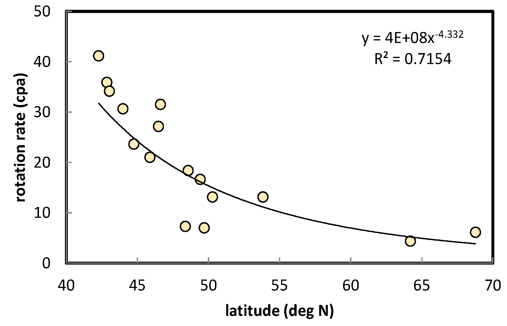
The latitudinal tendency is apparent in SWR rates shown in Figure 2, which results in a significant at the level α = 0.05 correlation with latitude. Latitudinal tendency in pan-Canadian data, nevertheless, appears subject to significant variability (R² = 0.2). This variability is caused by apparent outliers in Rocky Mountains and by the fact, that generally similar rotation rates are observed more to the North in Western Canada and more to the South in Eastern Canada, e.g., in the Prairies and in the Great Lakes region (which are located at different latitudes); similar pattern exists in Arctic Tundra (Figure 2). For this reason, it was decided to identify the meridional structure by limiting the continent-wide data to subsets from the 10°-wide N-S transects. A robust empirical relationship for the dependency of the SWR rate, ω*/2π, (cpa) on latitude, was derived from the least-squares fit to the data of the mid-continental N-S transect of 80.0°W–89.9°W (illustrated in Figure 4) and is given by:

ω* = 2π k_a φ^−4.33

(1)

where φ is latitude (degrees) and k_a is a units conversion factor (k_a = 4.0 × 10⁸ cpa/degree). Further analysis of correlation between spatial distribution of SWR and empirical relationship (1) was based on the Kendall test (instead of least-squares fit), because of its robustness with respect to outliers, skewness and curtosis [32], since all of these complicating factors were encountered in our small transect data subsets. The nonparametric Kendall test returns a significance of fit to SWR at the level of α_K = 0.01 with corresponding dispersion estimated by Kendall-tau τ_K = 0.72 in the illustrated transect. Similar strength of correlation (with Equation (1) and the same empirical parameters) is also present in five other transects (Table 1). However, SWR latitudinal dependence is absent in the Maritimes and Pacific Coast/Rockies.

Figure 4. SWR rate per annum (cpa) at CWEEDS stations versus latitude limited to a subset of data from the mid-continental 10°-wide (80.0°W–89.9°W) N-S transect. A polynomial trendline is added.

Figure 4. SWR rate per annum (cpa) at CWEEDS stations versus latitude limited to a subset of data from the mid-continental 10°-wide (80.0°W–89.9°W) N-S transect. A polynomial trendline is added.

The existence of a certain number of exceptions to the general rule of steady latitudinal dependent SWR makes it more logical to use an arbitrarily chosen dispersion threshold τ_K and to have the whole dataset divided into a “core” clearly latitude-dependent subset and a subset of “subtle exceptions”, which could be later classified with respect to their climatic and orographic signatures and location.

3.4. Identification of a “Core” Subset of Stations with Clear Latitudinal Dependence and Steadiness in SWR

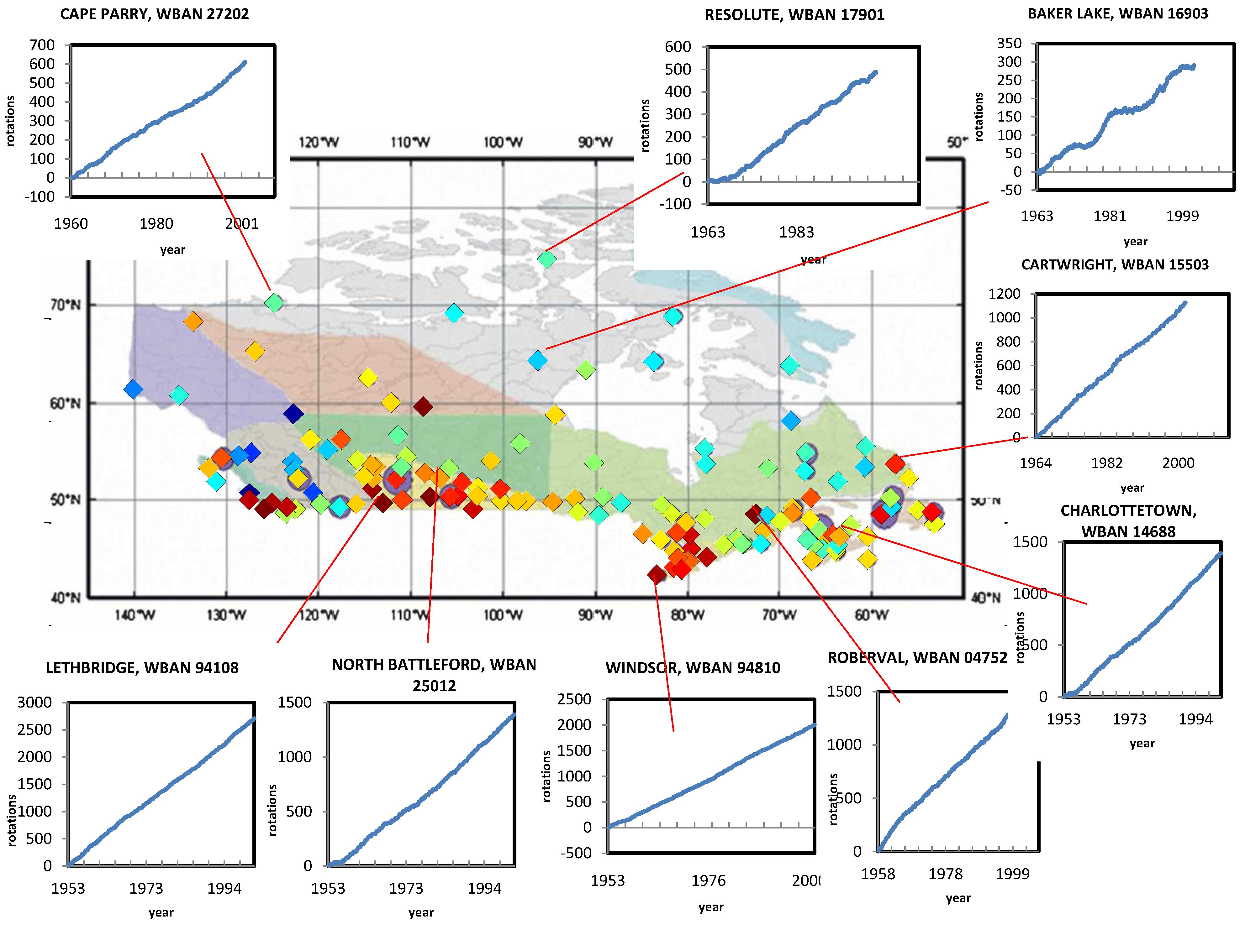
A “core” subset of stations where SWR exhibited both strong latitudinal dependency and steadiness was identified. Steadiness in SWR is important, as it means a constant asymmetry between cyclones and anticyclones. Latitudinal dependence is perhaps the more important of the two features of SWR, because it defines the SWR frequency in each particular location. We started with a subset of stations exhibiting clear latitudinal dependence of SWR, and proceeded to reassess the stationarity within this subset. The number of stations within the identified core subset (n = 118) provides a clear measure of the strength of the latitudinal dependency and steadiness of SWR. Nine illustrations are presented as inserted plots in Figure 5.

Figure 5. Nine examples from a set of 118 “core” stations, which strongly correlate with latitude (and also exhibit exemplary steady SWR). Inserts show temporal drift of historic wind direction angle in units of total rotations.

Figure 5. Nine examples from a set of 118 “core” stations, which strongly correlate with latitude (and also exhibit exemplary steady SWR). Inserts show temporal drift of historic wind direction angle in units of total rotations.

Exceptions (subtle exceptions) to the whole dataset were identified on the basis of goodness of fit of SWR to Equation (1) provided by Kendall tau τ_K. It was suggested, that Kendall tau τ_K = 0.4 represents sufficient criterion to the goodness of fit of the core subset to Equation (1), as it is similar to the goodness of fit observed in the 100.0°W–109.9°W N-S transect. Exclusion of locations, which are characterized by SWR rates more than three times different from the value provided by Equation (1) resulted in τ_K = 0.4 and these locations were considered subtle exceptions to the rule set by Equation (1) and to the whole dataset. This arbitrary criterion (τ_K = 0.4, or conversely the factor of 3 anomaly to Equation (1)) resulted in the identification of 6 stations that were rotating faster, and 25 stations that were rotating slower, than expected (including 1 slowing down to no net rotation, and 5 rotating negatively). In other words, 31 of the 149 stations (or 21% of the analyzed dataset) did not show a strong latitudinal dependency. In this context, it is important to specify that cases of extreme violation of the Equation (1), as shown by the 5 cases of negative cyclonic rotation (3%), are rare and narrowly confined to the Pacific Coast and adjacent Rockies. Nine illustrations of exceptions to latitudinal tendency and to steadiness of SWR (subtle exceptions) are presented as inserts in Figure 6. It is worth noting, that in this pan-Canadian classification (differently from Table 1 transect-based results) many stations from the 50°W–60°W and 120°W–140°W transects appear included in the core subset and conversely, some of the stations from 60°W to 120°W region were discarded as subtle exceptions.

Figure 6. Nine examples from 31 exceptions to latitudinal tendency and to steadiness of SWR shown in Figure 5. These subtle exceptions are faster than expected (at core stations), slower than expected and reverse, or cyclonic, rotations.

Figure 6. Nine examples from 31 exceptions to latitudinal tendency and to steadiness of SWR shown in Figure 5. These subtle exceptions are faster than expected (at core stations), slower than expected and reverse, or cyclonic, rotations.

The analysis shows that the core subset of stations (n = 118) exhibits exemplary steadiness in terms of anticyclonic rotation, with an SWR inter-annual variability characterized by R² > 0.9. Therefore, as a general rule, we suggest that continental SWR is very steady, anticyclonic, and latitudinal dependent.

4. Discussion

Our key finding is the observation of consistent anticyclonic rotation of wind direction at the continental surface (i.e., SWR) over Canada. Of the 149 Canadian meteostations analyzed, 97% exhibited anticyclonic SWR and 3% cyclonic SWR.

There are three main reasons why this deterministic SWR may not have been noted previously. Firstly, the phenomenon may be masked: (a) in the vicinity of large water bodies, i.e., in the Mediterranean or Pacific regions, by the sea breeze diurnal cycle, or (b) in regions dominated by prominent topographical features where singular wind patterns are found, as reflected in observations of cyclonic or unsteady SWR [21,22,23]. A second reason could lie in fitting of hodograph data to the diurnal cycle in previous studies, whereas the reality may be that slower SWR was overlooked, especially away from the sea breeze-dominated shoreline regions. Thirdly, the trend of steady SWR can only be observed over a long period, as demonstrated in Section 3.1 and the corresponding SWR frequency might not clearly dominate neighbouring frequencies in rotary spectra.

In line with previously published observations [21], we found that meteostations exhibiting negative cyclonic rotation (3%, or 5 out of 149 in our case) are located in regions subject to the influence of the ocean and/or the Rocky Mountains. Also, in relative contrast with the generally smooth continental pattern of SWR we also found the substantial variability of SWR rates at neighboring locations within this pattern, most likely caused by the orographic variability and associated frequently encountered wind channeling. The role of orography away from the Rocky Mountains merits investigation.

Regarding studies related to the SWR period it is important to reiterate, that Luo and colleagues [8,9] observed a planetary scale 16-day wave, which is typically pervasive during winter in mid and high latitudes in the middle atmosphere above Saskatoon, Canada. This planetary wave reoccurs with a period ranging from 12 to 24 days, as determined by medium-frequency radar measurements. Our SWR period at mid and high latitudes appears within the same LFV range; specifically, an SWR period in Saskatoon was observed to equal 14 days.

The frequency of SWR appears to be lower than that of synoptic events, and therefore SWR could be interpreted as being the basic asymmetry (or net anticyclonic imbalance) between cyclonic and anticyclonic events (e.g., caused by high and low pressure systems). No association of SWR frequency with the surface pressure at CWEEDS stations, analyzed by means of spectral analysis, has been established yet. Correspondingly the expansion of future analysis towards mid-atmospheric pressure systems seems important.

The stationarity over many decades of basic anticyclonic asymmetry manifested by SWR should be emphasized and is worth explanation. Another important feature of SWR is its spatial consistency combined with its dependence on latitude, likely pointing to the influence of the Coriolis force and its variation according to latitude (the beta-effect) via Rossby waves. If this is the case, a similar effect (anticyclonic rotation of continental winds) is expected in the Southern Hemisphere.

Observed periodicity could be associated with known periodic phenomena, like the weekend effect. For example, wherever the complete rotation of wind takes a week (i.e., in south of Canada), it is logical to expect that the anthropogenic air quality issues would appear in resonance with the established SWR phenomenon, whereas the magnitude of such effect requires evaluation in the future.

5. Conclusions

In summary, our study finds that:

• (1) The surface wind in most of Canada generally undergoes slow anticyclonic SWR, i.e., long-term, low-frequency periodicity beyond the synoptic scale, which represents a steady net imbalance of cyclonic and anticyclonic events (vortices).
• (2) The frequency of SWR was inversely correlated with latitude.
• (3) Of the meteostations analyzed, a small proportion (3%) exhibited negative (cyclonic) rotation in regions subject to the influence of the ocean and/or mountains.
• (4) The observed continental SWR appears to be deterministic, virtually ubiquitous, and highly persistent.
• (5) The role of orography and local meteorological forcings in SWR small-scale variability merits investigation.

References

- Mass, C.F.; Ovens, D.; Westrick, K.; Colle, B.A. Does increasing horizontal resolution produce more skillful forecasts? Bound. Lay. Meteorol. 2002, 83, 407–430. [Google Scholar]
- Horvath, K.; Koracin, D.; Vellore, R.; Jiang, J.; Belu, R. Sub-kilometer dynamical downscaling of near-surface winds in complex terrain using WRF and MM5 mesoscale models. J. Geophys. Res. 2012. [Google Scholar] [CrossRef]
- Stewart, J.Q.; Whiteman, C.D.; Steenburgh, W.J.; Bian, X. A climatological study of thermally driven wind systems of the US Intermountain West. Bull. Amer. Meteor. Soc. 2002, 83, 699–708. [Google Scholar] [CrossRef]
- Rife, D.L.; Davis, C.A.; Liu, Y.; Warner, T.T. Predictability of low-level winds by mesoscale meteorological models. Mon. Wea. Rev. 2004, 132, 2553–2569. [Google Scholar] [CrossRef]
- Seaman, N.L.; Gaudet, B.J.; Stauffer, D.R.; Mahrt, L.; Richardson, S.J.; Zielonka, J.R.; Wyngaard, J.C. Numerical prediction of submesoscale flow in the nocturnal stable boundary layer over complex terrain. Mon. Wea. Rev. 2012, 140, 956–977. [Google Scholar] [CrossRef]
- Bravo, M.; Mira, T.; Soler, M.R.; Cuxart, J. Intercomparison and evaluation of MM5 and Meso-NH mesoscale models in the stable boundary layer. Bound. Layer Meteorol. 2008, 128, 77–101. [Google Scholar] [CrossRef]
- Hamilton, K. General circulation model simulation of the structure and energetic of atmospheric models. Tellus 1987, 39A, 435–459. [Google Scholar] [CrossRef]
- Luo, Y.; Manson, A.H.; Meek, C.E.; Meyer, C.K.; Forbes, J.M. The quasi 16-day oscillations in the mesosphere and lower thermosphere at Saskatoon (52 N, 107 W), 1980-1996. J. Geophys. Res. 2000, 105, 2125–2138. [Google Scholar] [CrossRef]
- Luo, Y.; Hall, C.; Manson, A.H.; Meek, C.E.; Meyer, C.K.; Burrage, M.D.; Fritts, D.C.; Hocking, W.K.; MacDougall, J.; Riggin, D.M.; et al. The 16-day planetary waves: Multi-MF radar observations from the arctic to equator and comparisons with the HRDI measurements and the GSWM modelling results. Ann. Geophys. 2002, 20, 691–709. [Google Scholar] [CrossRef]
- Hodges, K.I.; Hoskins, B.J.; Boyle, J.; Thorncroft, C. A comparison of recent reanalysis datasets using objective feature tracking: Storm tracks and tropical easterly waves. Mon. Wea. Rev. 2003, 131, 2012–2037. [Google Scholar] [CrossRef]
- Wallace, J.M.; Lim, G.H.; Blackmon, M.L. Relationship between cyclone tracks, anticyclone tracks and baroclinic waveguides. J. Atmos. Sci. 1988, 45, 439–462. [Google Scholar] [CrossRef]
- Dell’Aquila, A.; Lucarini, V.; Ruti, P.M.; Calmanti, S. Hayashi spectra of the northern hemisphere mid-latitude atmospheric variability in the NCEP-NCAR and ECMWF reanalyses. Clim. Dynam. 2005, 25, 639–652. [Google Scholar] [CrossRef]
- Madden, R.A. Large-scale, free Rossby waves in the atmosphere-An update. Tellus 2007, 59A, 571–590. [Google Scholar]
- Chambers, F. The diurnal variations of the wind and barometric pressure at Bombay. Phil. Trans. R. Soc. 1873, 163, 1–18. [Google Scholar] [CrossRef]
- Haurwitz, B. Comments on the sea-breeze circulation. J. Meteor. 1947, 4, 1–8. [Google Scholar] [CrossRef]
- Neumann, J. On the rotation rate of the direction of sea and land breezes. J. Atmos. Sci. 1977, 34, 1913–1917. [Google Scholar] [CrossRef]
- Kusuda, M.; Alpert, P. Anticlockwise rotation of the wind hodograph. Part I: Theoretical study. J. Atmos. Sci. 1983, 40, 487–499. [Google Scholar] [CrossRef]
- Gille, S.T.; Llewellyn Smith, S.G.; Lee, S.M. Measuring the sea breeze from QuikSCAT scatterometry. Geophys. Res. Lett. 2003. [Google Scholar] [CrossRef]
- Kuo, A.C.; Polvani, L.M. Nonlinear geostrophic adjustment, cyclone/anticyclone asymmetry, and potential vorticity rearrangement. Phys. Fluids 2000, 12, 1087–1100. [Google Scholar] [CrossRef]
- Shipton, J. Balance, Gravity Waves and Jets in Turbulent Shallow Water Flows. Ph.D. Thesis, University of Sanit Andrews, Scotland, UK, 2009. [Google Scholar]
- Alpert, P.; Kusuda, M.; Abe, N. Anticlockwise rotation, eccentricity and tilt angle of the wind hodograph. Part II: An observational study. J. Atmos. Sci. 1984, 51, 3568–3583. [Google Scholar]
- Furberg, M.; Steyn, D.G.; Baldi, M. The climatology of sea breezes on Sardinia. Intl. J. Climatol. 2002, 22, 917–932. [Google Scholar]
- Sakazaki, T.; Fujiwara, M. Diurnal variations in summertime surface wind upon Japanese plains: Hodograph rotation and its dynamics. J. Meteor. Soc. Japan 2008, 86, 787–803. [Google Scholar] [CrossRef]
- Environment Canada. CWEEDS-Canadian Weather Energy and Engineering Data Set Files. Available online: ftp://arcdm20.tor.ec.gc.ca/pub/dist/climate/CWEEDS_2005/ (accessed on 23 November 2011).
- Fernandes, R.; Korolevych, V.; Wang, S. Trends in land evapotranspiration over Canada for the period 1960-2000 based on in situ climate observations and a land surface model. J. Hydrometeor. 2007, 8, 1016–1030. [Google Scholar] [CrossRef]
- Environment Canada. CDCD-Canadian Daily Climate Data 2 vols. Available online: ftp://arcdm20.tor.ec.gc.ca/pub/dist/CDCD/CDCD_DCQC_2007.zip (accessed on 23 November 2011).
- Mahrt, L. Surface wind direction variability. J. Appl. Meteor. Climatol. 2011, 50, 144–152. [Google Scholar] [CrossRef]
- Gonella, J. A rotary-component method for analysing meteorological and oceanographic vector time series. Deep-Sea Res. 1972, 19, 833–846. [Google Scholar]
- Emery, W.J.; Thomson, R.E. Data Analysis Methods in Physical Oceanography; Elsevier: Amsterdam, The Netherland, 2001; pp. 425–432. [Google Scholar]
- Theil, H. A rank-invariant method of linear and polynomial regression analysis. Indagationes. Math. 1950, 12, 85–91. [Google Scholar]
- Kendall, M.G. Rank Correlation Methods; Oxford University Press: Oxford, UK, 1975; p. 202. [Google Scholar]
- Hirsch, R.M.; Helsel, D.R.; Cohn, T.A.; Gilroy, E.J. Statistical Analysis of Hydrologic Data. In Handbook of Hydrology; McGraw-Hill: New York, NY, USA, 1993; p. 17. [Google Scholar]
© 2012 by the authors; licensee MDPI, Basel, Switzerland. This article is an open-access article distributed under the terms and conditions of the Creative Commons Attribution license (http://creativecommons.org/licenses/by/3.0/).
Share and Cite
MDPI and ACS Style
Korolevych, V.Y.; Richardson, R.B. Low-Frequency Rotation of Surface Winds over Canada. Atmosphere 2012, 3, 522-536. https://doi.org/10.3390/atmos3040522
AMA Style
Korolevych VY, Richardson RB. Low-Frequency Rotation of Surface Winds over Canada. Atmosphere. 2012; 3(4):522-536. https://doi.org/10.3390/atmos3040522
Chicago/Turabian StyleKorolevych, Vladimir Y., and Richard B. Richardson. 2012. "Low-Frequency Rotation of Surface Winds over Canada" Atmosphere 3, no. 4: 522-536. https://doi.org/10.3390/atmos3040522