<?xml version="1.0" encoding="UTF-8"?>
<!DOCTYPE article PUBLIC "-//NLM//DTD Journal Publishing DTD v2.3 20070202//EN" "journalpublishing.dtd">
<article xmlns:mml="http://www.w3.org/1998/Math/MathML" xmlns:xlink="http://www.w3.org/1999/xlink" xml:lang="en" article-type="research-article">
<front>
<journal-meta>
<journal-id journal-id-type="publisher-id">Atmosphere</journal-id>
<journal-title>Atmosphere</journal-title>
<issn pub-type="epub">2073-4433</issn>
<publisher>
<publisher-name>Molecular Diversity Preservation International (MDPI)</publisher-name></publisher></journal-meta>
<article-meta>
<article-id pub-id-type="doi">10.3390/atmos2030426</article-id>
<article-id pub-id-type="publisher-id">atmosphere-02-00426</article-id>
<article-categories>
<subj-group>
<subject>Article</subject></subj-group></article-categories>
<title-group>
<article-title>Chemical Data Assimilation—An Overview <xref ref-type="fn" rid="fn1-atmosphere-02-00426"><sup>‡</sup></xref></article-title></title-group>
<contrib-group>
<contrib contrib-type="author">
<name><surname>Sandu</surname><given-names>Adrian</given-names></name><xref ref-type="aff" rid="af1-atmosphere-02-00426"><sup>1</sup></xref><xref ref-type="corresp" rid="c1-atmosphere-02-00426"><sup>★</sup></xref></contrib>
<contrib contrib-type="author">
<name><surname>Chai</surname><given-names>Tianfeng</given-names></name><xref ref-type="aff" rid="af2-atmosphere-02-00426"><sup>2</sup></xref></contrib></contrib-group>
<aff id="af1-atmosphere-02-00426">
<label>1</label> Computational Science Laboratory, Department of Computer Science, Virginia Polytechnic Institute and State University, Blacksburg, VA 24061-0106, USA</aff>
<aff id="af2-atmosphere-02-00426">
<label>2</label> NOAA/OAR/ARL, Silver Spring Metro Center #3, Rm. 3437, 1315 East West Highway, Silver Spring, MD 20910, USA; E-Mail: <email>Tianfeng.Chai@noaa.gov</email></aff>
<author-notes>
<corresp id="c1-atmosphere-02-00426">
<label>★</label> Author to whom correspondence should be addressed; E-Mail: <email>Sandu@cs.vt.edu</email>; Tel.: +1-(540)-231-2193; Fax: +1-(540)-231-9218.</corresp></author-notes>
<pub-date pub-type="collection">
<year>2011</year></pub-date>
<pub-date pub-type="epub">
<day>29</day>
<month>08</month>
<year>2011</year></pub-date>
<volume>2</volume>
<issue>3</issue>
<fpage>426</fpage>
<lpage>463</lpage>
<history>
<date date-type="received">
<day>07</day>
<month>06</month>
<year>2011</year></date>
<date date-type="rev-recd">
<day>09</day>
<month>08</month>
<year>2011</year></date>
<date date-type="accepted">
<day>19</day>
<month>08</month>
<year>2011</year></date></history>
<permissions>
<copyright-statement>© 2011 by the authors; licensee MDPI, Basel, Switzerland.</copyright-statement>
<copyright-year>2011</copyright-year>
<license>
<p>This article is an open access article distributed under the terms and conditions of the Creative Commons Attribution license (http://creativecommons.org/licenses/by/3.0/.)</p></license></permissions>
<abstract>
<p>Chemical data assimilation is the process by which models use measurements to produce an optimal representation of the chemical composition of the atmosphere. Leveraging advances in algorithms and increases in the available computational power, the integration of numerical predictions and observations has started to play an important role in air quality modeling. This paper gives an overview of several methodologies used in chemical data assimilation. We discuss the Bayesian framework for developing data assimilation systems, the suboptimal and the ensemble Kalman filter approaches, the optimal interpolation (OI), and the three and four dimensional variational methods. Examples of assimilation real observations with CMAQ model are presented.</p></abstract>
<kwd-group>
<kwd>chemical transport modeling</kwd>
<kwd>data assimilation</kwd>
<kwd>Kalman filter</kwd>
<kwd>variational methods</kwd></kwd-group></article-meta></front>
<body>
<sec sec-type="intro">
<label>1.</label>
<title>Introduction</title>
<p>Chemical data assimilation produces improved estimates of the chemical state of the atmosphere by combining information from three different sources: the physical and chemical laws of evolution (encapsulated in the model), the reality (as captured by the observations), and the current best estimate of the distribution of pollutants in the atmosphere (encapsulated in the prior) – all with associated errors [<xref ref-type="bibr" rid="b1-atmosphere-02-00426">1</xref>]. Considerable experience with data assimilation has been accumulated in the fields of numerical weather prediction, ocean modeling, and oil reservoir simulation [<xref ref-type="bibr" rid="b2-atmosphere-02-00426">2</xref>–<xref ref-type="bibr" rid="b7-atmosphere-02-00426">7</xref>]. Chemical data assimilation has started to play an important role in the atmospheric composition studies, and many successful applications illustrate its benefits [<xref ref-type="bibr" rid="b8-atmosphere-02-00426">8</xref>–<xref ref-type="bibr" rid="b18-atmosphere-02-00426">18</xref>]. These benefits include improved initial and boundary conditions, and refined top-down emission estimates, all contributing to better air quality forecasts. Chemical data assimilation poses specific challenges related to the multiple physical processes included in models, the stiffness of chemical equations, the sparseness of chemical observations, and the uncertainty in the anthropogenic and natural emission levels.</p>
<p>The chemical interactions take place on a wide range of temporal scales (from milliseconds to days). This makes the system numerically stiff. The concentrations of short lived radical species follow the concentrations of long lived species through quasi steady state relations. After a short time the chemical evolution collapses onto a low dimensional manifold in state space. As a consequence, when meteorological fields are computed off line, ensembles of simulations will tend to converge to the same trajectory. Moreover, a direct adjustment of radical species through data assimilation is not feasible.</p>
<p>In regional air quality simulations, the influence of the initial conditions fades in time, and the concentration fields become largely driven by emission and removal processes (and by lateral boundary conditions in regional simulations). Therefore, to improve the analysis capabilities of CTMs, it is necessary to consider the estimation of emission parameters and lateral boundaries through data assimilation [<xref ref-type="bibr" rid="b19-atmosphere-02-00426">19</xref>,<xref ref-type="bibr" rid="b20-atmosphere-02-00426">20</xref>]. Moreover, both the anthropologic and natural emissions are poorly constrained (<italic>i.e</italic>., the prior information on emissions is highly uncertain). This makes the top down estimation of emissions a challenging computational problem. Chemical transport models are often characterized by non negligible biases, and data assimilation can benefit from bias correction schemes [<xref ref-type="bibr" rid="b21-atmosphere-02-00426">21</xref>].</p>
<p>Chemical observations are still sparse, as the network is not as extensive as that used in numerical weather prediction. Local observations of chemical and particulate concentrations are strongly influenced by the local variability, yet they are used to constrain large scale three dimensional fields. Recently there has a considerable growth in the available remote sensing (satellite) data on tracer concentrations. This data is characterized by non-negligible biases; a method to alleviate this issue is proposed in [<xref ref-type="bibr" rid="b22-atmosphere-02-00426">22</xref>], where a single coherent dataset is created from all available ozone column measurements.</p>
<p>An additional difficulty arises from the multiphysics nature of the simulation, where the evolution is driven by multiple competing physical processes. A successful data assimilation system need to correctly account for error correlations between chemical species (due to chemical interactions) and between chemical and dynamic variables (due to transport processes).</p>
<p>This paper gives an overview of the state of the art in chemical data assimilation. We review chemical transport models in Section 1.1 and chemical observations in Section 1.2. Section 2 is devoted to the formulation of the chemical data assimilation problem in a Bayesian framework. Practical assimilation methods discussed include optimal interpolation (OI) (Section 3.3), suboptimal Kalman filters (Section 3.2), ensemble Kalman filters (Section 3.4), three dimensional variational (3D-Var, Section 3.5) and four dimensional variational data assimilation (4D-Var, Section 3.6). Challenges to chemical data assimilation such as data inputs, the construction of adjoints, and the construction of error covariance matrices are highlighted in Section 4. Assimilation results with real data and the CMAQ model are presented in Section 5. Section 6 draws conclusions and pinpoints to future directions in chemical data assimilation.</p>
<sec>
<label>1.1.</label>
<title>Chemical Transport Models</title>
<p>An atmospheric chemical transport model (CTM) solves the mass balance equations for concentrations x<sub>(</sub><italic><sub>i</sub></italic><sub>)</sub> of tracer species 1 ≤ <italic>i</italic> ≤ <italic>s</italic>. The tracer species can be in gas, liquid, or particulate phases, and their concentrations are continuously changed by multiple physical and chemical processes,
<disp-formula id="FD1">
<label>(1)</label>
<mml:math id="mm1" display="block">
<mml:semantics id="sm1">
<mml:mrow>
<mml:mtable columnalign="left">
<mml:mtr columnalign="left">
<mml:mtd columnalign="left">
<mml:mrow>
<mml:mtable columnalign="left">
<mml:mtr columnalign="left">
<mml:mtd columnalign="left">
<mml:mrow>
<mml:mfrac>
<mml:mrow>
<mml:mo>∂</mml:mo>
<mml:msub>
<mml:mtext>x</mml:mtext>
<mml:mrow>
<mml:mo stretchy="false">(</mml:mo>
<mml:mi>i</mml:mi>
<mml:mo stretchy="false">)</mml:mo></mml:mrow></mml:msub></mml:mrow>
<mml:mrow>
<mml:mo>∂</mml:mo>
<mml:mi>t</mml:mi></mml:mrow></mml:mfrac>
<mml:mo>=</mml:mo>
<mml:mo>−</mml:mo>
<mml:mi>u</mml:mi>
<mml:mo>⋅</mml:mo>
<mml:mo>∇</mml:mo>
<mml:msub>
<mml:mtext>x</mml:mtext>
<mml:mrow>
<mml:mo stretchy="false">(</mml:mo>
<mml:mi>i</mml:mi>
<mml:mo stretchy="false">)</mml:mo></mml:mrow></mml:msub>
<mml:mo>+</mml:mo>
<mml:mfrac>
<mml:mn>1</mml:mn>
<mml:mo mathvariant="italic">ρ</mml:mo></mml:mfrac>
<mml:mo>∇</mml:mo>
<mml:mo>⋅</mml:mo>
<mml:mo stretchy="false">(</mml:mo>
<mml:mo mathvariant="italic">ρ</mml:mo>
<mml:mi>K</mml:mi>
<mml:mo>∇</mml:mo>
<mml:msub>
<mml:mtext>x</mml:mtext>
<mml:mrow>
<mml:mo stretchy="false">(</mml:mo>
<mml:mi>i</mml:mi>
<mml:mo stretchy="false">)</mml:mo></mml:mrow></mml:msub>
<mml:mo stretchy="false">)</mml:mo>
<mml:mo>+</mml:mo>
<mml:mfrac>
<mml:mn>1</mml:mn>
<mml:mo mathvariant="italic">ρ</mml:mo></mml:mfrac>
<mml:msub>
<mml:mi>f</mml:mi>
<mml:mrow>
<mml:mo stretchy="false">(</mml:mo>
<mml:mi>i</mml:mi>
<mml:mo stretchy="false">)</mml:mo></mml:mrow></mml:msub>
<mml:mo stretchy="false">(</mml:mo>
<mml:mo mathvariant="italic">ρ</mml:mo>
<mml:mtext>x</mml:mtext>
<mml:mo stretchy="false">)</mml:mo>
<mml:mo>+</mml:mo>
<mml:msub>
<mml:mi>E</mml:mi>
<mml:mrow>
<mml:mo stretchy="false">(</mml:mo>
<mml:mi>i</mml:mi>
<mml:mo stretchy="false">)</mml:mo></mml:mrow></mml:msub>
<mml:mo>,</mml:mo></mml:mrow></mml:mtd>
<mml:mtd columnalign="left">
<mml:mrow>
<mml:mn>1</mml:mn>
<mml:mo>≤</mml:mo>
<mml:mi>i</mml:mi>
<mml:mo>≤</mml:mo>
<mml:mi>s</mml:mi>
<mml:mo>,</mml:mo></mml:mrow></mml:mtd>
<mml:mtd columnalign="left">
<mml:mrow>
<mml:msub>
<mml:mi>t</mml:mi>
<mml:mn>0</mml:mn></mml:msub>
<mml:mo>≤</mml:mo>
<mml:mi>t</mml:mi>
<mml:mo>≤</mml:mo>
<mml:msub>
<mml:mi>t</mml:mi>
<mml:mi>F</mml:mi></mml:msub></mml:mrow></mml:mtd></mml:mtr></mml:mtable></mml:mrow></mml:mtd></mml:mtr>
<mml:mtr columnalign="left">
<mml:mtd columnalign="left">
<mml:mrow>
<mml:msub>
<mml:mtext>x</mml:mtext>
<mml:mrow>
<mml:mo stretchy="false">(</mml:mo>
<mml:mi>i</mml:mi>
<mml:mo stretchy="false">)</mml:mo></mml:mrow></mml:msub>
<mml:mo stretchy="false">(</mml:mo>
<mml:msub>
<mml:mi>t</mml:mi>
<mml:mn>0</mml:mn></mml:msub>
<mml:mo>,</mml:mo>
<mml:mi>x</mml:mi>
<mml:mo stretchy="false">)</mml:mo>
<mml:mo>=</mml:mo>
<mml:msubsup>
<mml:mtext>x</mml:mtext>
<mml:mrow>
<mml:mo stretchy="false">(</mml:mo>
<mml:mi>i</mml:mi>
<mml:mo stretchy="false">)</mml:mo></mml:mrow>
<mml:mrow>
<mml:mtext>initial</mml:mtext></mml:mrow></mml:msubsup>
<mml:mo stretchy="false">(</mml:mo>
<mml:mi>x</mml:mi>
<mml:mo stretchy="false">)</mml:mo></mml:mrow></mml:mtd></mml:mtr>
<mml:mtr columnalign="left">
<mml:mtd columnalign="left">
<mml:mrow>
<mml:mtable columnalign="left">
<mml:mtr columnalign="left">
<mml:mtd columnalign="left">
<mml:mrow>
<mml:msub>
<mml:mtext>x</mml:mtext>
<mml:mrow>
<mml:mo stretchy="false">(</mml:mo>
<mml:mi>i</mml:mi>
<mml:mo stretchy="false">)</mml:mo></mml:mrow></mml:msub>
<mml:mo stretchy="false">(</mml:mo>
<mml:mi>t</mml:mi>
<mml:mo>,</mml:mo>
<mml:mi>x</mml:mi>
<mml:mo stretchy="false">)</mml:mo>
<mml:mo>=</mml:mo>
<mml:msubsup>
<mml:mtext>x</mml:mtext>
<mml:mrow>
<mml:mo stretchy="false">(</mml:mo>
<mml:mi>i</mml:mi>
<mml:mo stretchy="false">)</mml:mo></mml:mrow>
<mml:mrow>
<mml:mtext>inflow</mml:mtext></mml:mrow></mml:msubsup>
<mml:mo stretchy="false">(</mml:mo>
<mml:mi>t</mml:mi>
<mml:mo>,</mml:mo>
<mml:mi>x</mml:mi>
<mml:mo stretchy="false">)</mml:mo></mml:mrow></mml:mtd>
<mml:mtd columnalign="left">
<mml:mrow>
<mml:mtext>on</mml:mtext></mml:mrow></mml:mtd>
<mml:mtd columnalign="left">
<mml:mrow>
<mml:msup>
<mml:mo>Γ</mml:mo>
<mml:mrow>
<mml:mtext>inflow</mml:mtext></mml:mrow></mml:msup></mml:mrow></mml:mtd></mml:mtr></mml:mtable></mml:mrow></mml:mtd></mml:mtr>
<mml:mtr columnalign="left">
<mml:mtd columnalign="left">
<mml:mrow>
<mml:mtable columnalign="left">
<mml:mtr columnalign="left">
<mml:mtd columnalign="left">
<mml:mrow>
<mml:msub>
<mml:mi>K</mml:mi>
<mml:mrow>
<mml:mi>n</mml:mi>
<mml:mi>n</mml:mi></mml:mrow></mml:msub>
<mml:mfrac>
<mml:mrow>
<mml:mo>∂</mml:mo>
<mml:msub>
<mml:mtext>x</mml:mtext>
<mml:mrow>
<mml:mo stretchy="false">(</mml:mo>
<mml:mi>i</mml:mi>
<mml:mo stretchy="false">)</mml:mo></mml:mrow></mml:msub></mml:mrow>
<mml:mrow>
<mml:mo>∂</mml:mo>
<mml:mi>n</mml:mi></mml:mrow></mml:mfrac>
<mml:mo>=</mml:mo>
<mml:mn>0</mml:mn></mml:mrow></mml:mtd>
<mml:mtd columnalign="left">
<mml:mrow>
<mml:mtext>on</mml:mtext></mml:mrow></mml:mtd>
<mml:mtd columnalign="left">
<mml:mrow>
<mml:msup>
<mml:mo>Γ</mml:mo>
<mml:mrow>
<mml:mtext>outflow</mml:mtext></mml:mrow></mml:msup></mml:mrow></mml:mtd></mml:mtr></mml:mtable></mml:mrow></mml:mtd></mml:mtr>
<mml:mtr columnalign="left">
<mml:mtd columnalign="left">
<mml:mrow>
<mml:mtable columnalign="left">
<mml:mtr columnalign="left">
<mml:mtd columnalign="left">
<mml:mrow>
<mml:msub>
<mml:mi>K</mml:mi>
<mml:mrow>
<mml:mi>n</mml:mi>
<mml:mi>n</mml:mi></mml:mrow></mml:msub>
<mml:mfrac>
<mml:mrow>
<mml:mo>∂</mml:mo>
<mml:msub>
<mml:mtext>x</mml:mtext>
<mml:mrow>
<mml:mo stretchy="false">(</mml:mo>
<mml:mi>i</mml:mi>
<mml:mo stretchy="false">)</mml:mo></mml:mrow></mml:msub></mml:mrow>
<mml:mrow>
<mml:mo>∂</mml:mo>
<mml:mi>n</mml:mi></mml:mrow></mml:mfrac>
<mml:mo>=</mml:mo>
<mml:msubsup>
<mml:mi>V</mml:mi>
<mml:mrow>
<mml:mo stretchy="false">(</mml:mo>
<mml:mi>i</mml:mi>
<mml:mo stretchy="false">)</mml:mo></mml:mrow>
<mml:mrow>
<mml:mtext>deposition</mml:mtext></mml:mrow></mml:msubsup>
<mml:msub>
<mml:mi>x</mml:mi>
<mml:mrow>
<mml:mo stretchy="false">(</mml:mo>
<mml:mi>i</mml:mi>
<mml:mo stretchy="false">)</mml:mo></mml:mrow></mml:msub>
<mml:mo>−</mml:mo>
<mml:msub>
<mml:mi>Q</mml:mi>
<mml:mrow>
<mml:mo stretchy="false">(</mml:mo>
<mml:mi>i</mml:mi>
<mml:mo stretchy="false">)</mml:mo></mml:mrow></mml:msub></mml:mrow></mml:mtd>
<mml:mtd columnalign="left">
<mml:mrow>
<mml:mtext>on</mml:mtext></mml:mrow></mml:mtd>
<mml:mtd columnalign="left">
<mml:mrow>
<mml:msup>
<mml:mo>Γ</mml:mo>
<mml:mrow>
<mml:mtext>ground</mml:mtext></mml:mrow></mml:msup></mml:mrow></mml:mtd></mml:mtr></mml:mtable></mml:mrow></mml:mtd></mml:mtr></mml:mtable></mml:mrow></mml:semantics></mml:math></disp-formula></p>
<p>Here <italic>u</italic> represents the wind velocity vector, <italic>K</italic> is the turbulent diffusion tensor, and <italic>ρ</italic> is the air density These variables are typically prescribed from simulations with a numerical weather prediction model, or are part of the prognostic variables for meteorological models with online chemistry. The concentrations x<sub>(</sub><italic><sub>i</sub></italic><sub>)</sub> are expressed as a mole fraction (e.g., the number of molecules of tracer per 1 billion molecules of air); the absolute concentration of tracer <italic>i</italic> is <italic>ρ</italic>x<sub>(</sub><italic><sub>i</sub></italic><sub>)</sub> (molecules/cm<sup>3</sup>). <italic>f</italic><sub>(</sub><italic><sub>i</sub></italic><sub>)</sub> is the rate of transformations of species i and depends on all other concentrations at the same spatial location. Such local transformations are determined by gas and liquid phase chemical kinetics, by inter-phase mass transfer, by aerosol dynamic processes (coagulation and growth), by thermodynamic processes, <italic>etc.</italic> The elevated emissions of species <italic>i</italic> are <italic>E</italic><sub>(</sub><italic><sub>i</sub></italic><sub>)</sub> and the ground level emissions are <italic>Q</italic><sub>(</sub><italic><sub>i</sub></italic><sub>)</sub>. The deposition velocity is 
<inline-formula>
<mml:math id="mm2" display="inline">
<mml:semantics id="sm2">
<mml:mrow>
<mml:msubsup>
<mml:mi>V</mml:mi>
<mml:mrow>
<mml:mo stretchy="false">(</mml:mo>
<mml:mi>i</mml:mi>
<mml:mo stretchy="false">)</mml:mo></mml:mrow>
<mml:mrow>
<mml:mtext>deposition</mml:mtext></mml:mrow></mml:msubsup></mml:mrow></mml:semantics></mml:math></inline-formula>. The model has prescribed initial conditions x<sup>initial</sup>, and is subject to Neumann boundary conditions [<xref ref-type="bibr" rid="b23-atmosphere-02-00426">23</xref>] at the ground level boundary Γ<sup>ground</sup>. Dirichlet boundary conditions [<xref ref-type="bibr" rid="b23-atmosphere-02-00426">23</xref>] are imposed at the inflow boundary Γ<sup>inflow</sup> (along the top and, for regional models, along the lateral boundary as well). A no diffusive flow condition is imposed at the outflow boundary Γ<sup>outflow</sup> (along the top and, for regional models, along the lateral boundary as well).</p>
<p>The numerical solution to <xref rid="FD1" ref-type="disp-formula">(1)</xref> is represented by the discrete model
<disp-formula id="FD2">
<label>(2)</label>
<mml:math id="mm3" display="block">
<mml:semantics id="sm3">
<mml:mrow>
<mml:mtable>
<mml:mtr>
<mml:mtd>
<mml:mrow>
<mml:msub>
<mml:mtext>x</mml:mtext>
<mml:mi>i</mml:mi></mml:msub>
<mml:mo>=</mml:mo>
<mml:msub>
<mml:mo>ℳ</mml:mo>
<mml:mrow>
<mml:msub>
<mml:mi>t</mml:mi>
<mml:mrow>
<mml:mi>i</mml:mi>
<mml:mo>−</mml:mo>
<mml:mn>1</mml:mn></mml:mrow></mml:msub>
<mml:mo>→</mml:mo>
<mml:msub>
<mml:mi>t</mml:mi>
<mml:mi>i</mml:mi></mml:msub></mml:mrow></mml:msub>
<mml:mo stretchy="false">(</mml:mo>
<mml:mi>u</mml:mi>
<mml:mo>,</mml:mo>
<mml:mi>K</mml:mi>
<mml:mo>,</mml:mo>
<mml:mi>E</mml:mi>
<mml:mo>,</mml:mo>
<mml:mi>Q</mml:mi>
<mml:mo>,</mml:mo>
<mml:msup>
<mml:mi>V</mml:mi>
<mml:mrow>
<mml:mtext>deposition</mml:mtext></mml:mrow></mml:msup>
<mml:mo>,</mml:mo>
<mml:msup>
<mml:mtext>x</mml:mtext>
<mml:mrow>
<mml:mtext>inflow</mml:mtext></mml:mrow></mml:msup>
<mml:mo>;</mml:mo>
<mml:msub>
<mml:mtext>x</mml:mtext>
<mml:mrow>
<mml:mi>i</mml:mi>
<mml:mo>−</mml:mo>
<mml:mn>1</mml:mn></mml:mrow></mml:msub>
<mml:mo stretchy="false">)</mml:mo>
<mml:mo>,</mml:mo></mml:mrow></mml:mtd>
<mml:mtd>
<mml:mrow>
<mml:mi>i</mml:mi>
<mml:mo>=</mml:mo>
<mml:mn>1</mml:mn>
<mml:mo>,</mml:mo>
<mml:mn>2</mml:mn>
<mml:mo>,</mml:mo>
<mml:mo>…</mml:mo>
<mml:mo>;</mml:mo></mml:mrow></mml:mtd>
<mml:mtd>
<mml:mrow>
<mml:msub>
<mml:mtext>x</mml:mtext>
<mml:mn>0</mml:mn></mml:msub>
<mml:mo>=</mml:mo>
<mml:msup>
<mml:mtext>x</mml:mtext>
<mml:mrow>
<mml:mtext>initial</mml:mtext></mml:mrow></mml:msup></mml:mrow></mml:mtd></mml:mtr></mml:mtable></mml:mrow></mml:semantics></mml:math></disp-formula></p>
<p>In (2), the solution x<italic><sub>i</sub></italic> is the discrete state vector containing the concentrations of chemical species sampled at the grid points at time <italic>t<sub>i</sub></italic>. The discrete initial condition x<sub>0</sub> is obtained by sampling x<sup>initial</sup> at the grid points. The model solution operator ℳ depends on model parameters such as emission rates, deposition velocities, and boundary fluxes. In principle, all the model parameters, as well as the initial conditions x<sub>0</sub>, can be retrieved through data assimilation if there are enough observations. However, we have to limit the number of model parameters to be determined as the observations in reality are lacking to accurately constrain the problem.</p>
<p>While there are numerous CTMs available for both regional and global applications, the community Multiscale Air Quality (CMAQ) model is primarily used to provide examples in Section 5. As an open-source community model, CMAQ is widely used by the air quality community worldwide and continuously updated with support from the U.S. Environmental Protection Agency (EPA) and Community Modeling &amp; Analysis System (CMAS) [<xref ref-type="bibr" rid="b24-atmosphere-02-00426">24</xref>]. CMAQ model was developed by the U.S. EPA to meet the needs of both environmental managers and scientists to improve their ability to evaluate the impact of air quality management practices and to probe, understand, and simulate chemical and physical interactions in the atmosphere. CMAQ model has been designed to model multiple air quality issues, such as tropospheric ozone, fine particles, toxics, acid deposition, and visibility degradation as a whole; and it has capabilities to solve air quality problems in multiple scales including the urban and regional scales [<xref ref-type="bibr" rid="b25-atmosphere-02-00426">25</xref>,<xref ref-type="bibr" rid="b26-atmosphere-02-00426">26</xref>]. CMAQ has been used in numerous chemical data assimilation studies. A 4D-Var data assimilation system, including an adjoint model for CMAQ, has been developed for version 4.5 [<xref ref-type="bibr" rid="b27-atmosphere-02-00426">27</xref>]. The assimilation of AIRNow ozone observations [<xref ref-type="bibr" rid="b28-atmosphere-02-00426">28</xref>] proved to be beneficial for improving ozone predictions [<xref ref-type="bibr" rid="b29-atmosphere-02-00426">29</xref>]. Zubrow <italic>et al.</italic> [<xref ref-type="bibr" rid="b30-atmosphere-02-00426">30</xref>] presented an ensemble adjustment Kalman filter (EAKF) approach using a a single tracer version of the CMAQ model to assimilate surface measurements of carbon monoxide and showed its ability to provide skillful model results.</p></sec>
<sec>
<label>1.2.</label>
<title>Chemical Observations</title>
<p>Measurements of atmospheric chemical fields have been significantly increasing for the past years throughout the world. Many ground-based networks have been established to routinely monitor the air quality on the surface level. For instance, in the U.S. the AIRNow network has been reporting ozone and fine particle observation (PM2.5, <italic>i.e</italic>., particulate matter less than 2.5 micrometers in diameter) in near-real-time [<xref ref-type="bibr" rid="b28-atmosphere-02-00426">28</xref>]. However, surface measurements have to be combined with vertical profiles to obtain the three-dimensional states of the atmospheric constituents. Jeuken <italic>et al.</italic> shows that assimilating ozone columns alone has little impact on the shape of the vertical ozone profile which is mainly determined by the transport [<xref ref-type="bibr" rid="b31-atmosphere-02-00426">31</xref>]. To complement the surface measurements, there are observations regularly taken by balloon and lidar networks. In adding the vertical profiles the chemical and dynamical processes of the atmospheric chemistry can be better understood. Such networks include SHADOZ (Southern Hemisphere Additional Ozonesondes) which has operated since 1998 [<xref ref-type="bibr" rid="b32-atmosphere-02-00426">32</xref>–<xref ref-type="bibr" rid="b34-atmosphere-02-00426">34</xref>]. Lidar networks contribute to the atmospheric chemistry studies by providing vertically resolved data in an extended area. Using observations from 14 Japan National Institute for Environmental Studies (NIES) lidars [<xref ref-type="bibr" rid="b35-atmosphere-02-00426">35</xref>] and RAMS/CFORS-4DVAR assimilation system, Yumimoto <italic>et al.</italic> investigated mineral dust transport and emission in East Asia during a spring dust event in 2007 [<xref ref-type="bibr" rid="b36-atmosphere-02-00426">36</xref>].</p>
<p>In addition to the in-situ measurement networks, multiple satellite instruments with capability to measure the troposphere and stratosphere atmospheric chemical fields have been operating to provide real-time measurements [<xref ref-type="bibr" rid="b37-atmosphere-02-00426">37</xref>,<xref ref-type="bibr" rid="b38-atmosphere-02-00426">38</xref>]. For instance, Aura [<xref ref-type="bibr" rid="b39-atmosphere-02-00426">39</xref>], a multi-national NASA Earth Observing System (EOS) satellite to study atmospheric chemistry following Terra (launched in 1999) and Aqua (launched in 2002), was launched in 2004. Aura carries a High Resolution Dynamics Limb Sounder (HIRDLS, which stopped operating in 2008), an Ozone Monitoring Instrument (OMI), a Tropospheric Emission Spectrometer (TES), and a Microwave Limb Sounder (MLS) [<xref ref-type="bibr" rid="b40-atmosphere-02-00426">40</xref>]. The retrieval of Envisat-SCIAMACHY (Scanning Imaging Absorption Spectrometer for Atmospheric Chartography) by European Space Agency provides various atmospheric constituents [<xref ref-type="bibr" rid="b41-atmosphere-02-00426">41</xref>]. Moderate resolution imaging spectroradiometer (MODIS) aboard Terra (EOS AM) and Aqua (EOS PM) satellites provides near real time aerosol optical depth (AOD) observations with good spatial resolution and coverage [<xref ref-type="bibr" rid="b42-atmosphere-02-00426">42</xref>,<xref ref-type="bibr" rid="b43-atmosphere-02-00426">43</xref>] and they have been used in many aerosol assimilation applications [<xref ref-type="bibr" rid="b44-atmosphere-02-00426">44</xref>–<xref ref-type="bibr" rid="b47-atmosphere-02-00426">47</xref>]. One of the earlist efforts in chemical data assimilation was a OI type statistical analysis scheme to assimilate the Total Ozone Mapping Spectrometer (TOMS) total ozone data and the Solar Backscatter Ultraviolet/2 (SBUV/2) partial ozone profile observations into an off-line ozone transport model by Štajner <italic>et al.</italic> [<xref ref-type="bibr" rid="b48-atmosphere-02-00426">48</xref>]. With a broad horizontal coverage, satellite observations are complementary to in-situ measurements that are often located at places of interest. Nassar <italic>et al.</italic> showed the benefit of combining the two types of observations together in chemical data assimilation systems by assimilating both satellite observations of <italic>CO</italic><sub>2</sub> from TES and surface flask measurements [<xref ref-type="bibr" rid="b49-atmosphere-02-00426">49</xref>].</p>
<p>In recent years, many field experiments have been carried out with intensive measurement activities. For instance, the International Consortium for Atmospheric Research on Transport and Transformation (ICARTT) field campaign took place in the northeastern United States and the Maritime Provinces of Canada during summer 2004 [<xref ref-type="bibr" rid="b50-atmosphere-02-00426">50</xref>]. Over 300 government-agency and university participants from U.S., Canada, UK, Germany, and France carried out eleven independent but highly coordinated field experiments with various objectives. Among them, the U.S. National Oceanic and Atmospheric Administration (NOAA) New England Air Quality Study - Intercontinental Transport and Chemical Transformation [<xref ref-type="bibr" rid="b51-atmosphere-02-00426">51</xref>] 2004 experiment studied air quality along the Eastern Seaboard and transport of North American emissions into the North Atlantic [<xref ref-type="bibr" rid="b52-atmosphere-02-00426">52</xref>]. The European International Transport of Ozone and Precursors (EU-ITOP) field program aimed at understanding the factors determining air quality over America and Europe and over remote regions of the North Atlantic [<xref ref-type="bibr" rid="b53-atmosphere-02-00426">53</xref>,<xref ref-type="bibr" rid="b54-atmosphere-02-00426">54</xref>]. As another component of ICARTT, NASA Intercontinental Chemical Transport Experiment - North America Phase A (INTEX-A), focused on the transport and transformation of gases and aerosols on transcontinental/intercontinental scales and their impact on air quality and climate. The continued NASA INTEX project, Phase B, coincided with MIRAGE-Mex (Megacities Impact on Regional and Global Environment-Mexico) in the spring of 2006 [<xref ref-type="bibr" rid="b55-atmosphere-02-00426">55</xref>,<xref ref-type="bibr" rid="b56-atmosphere-02-00426">56</xref>]. In the field experiments, coordinated measurements were made by multiple in-situ instruments on board aircrafts in flights, additional ozonesondes on ground or a research vessel, and airborne ozone lidars. Using ICARTT/INTEX-A data, Chai <italic>et al.</italic> [<xref ref-type="bibr" rid="b11-atmosphere-02-00426">11</xref>] shows that the combined ozone observations provide a much better representation of the ozone distributions when assimilated simultaneously.</p></sec>
<sec>
<label>1.3.</label>
<title>Chemical Data Assimilation</title>
<p>We now summarize some of the previous work in the field of chemical data assimilation. The field has accumulated a large body of work from contributions by many authors. Among those, many excellent papers were products of the Global and Regional Earth-System Monitoring Using Satellite and In situ Data (GEMS [<xref ref-type="bibr" rid="b57-atmosphere-02-00426">57</xref>]) project funded by European Commission to develop comprehensive data analysis and modelling systems for greenhouse gases, global reactive gases, and aerosol, with a focus on Europe from March 2005 to May 2009. Since June 2009, GEMS and the Protocol Monitoring for the GMES Service Element: Atmosphere (PROMOTE [<xref ref-type="bibr" rid="b58-atmosphere-02-00426">58</xref>]) merged into Monitoring Atmospheric Composition and Climate (MACC [<xref ref-type="bibr" rid="b59-atmosphere-02-00426">59</xref>]) project to continue the operation and improvement of the forecasting and assimilation developed during GEMS [<xref ref-type="bibr" rid="b60-atmosphere-02-00426">60</xref>]. Some excellent previous work will inevitably end up not being included in this paper's citation list, and we apologize for this.</p>
<p>Two approaches to data assimilation have become widely used in applications: variational methods, rooted in control theory, and Kalman filter methods, rooted in statistical estimation theory. The base concepts of the variational approach to chemical data assimilation are discussed in [<xref ref-type="bibr" rid="b1-atmosphere-02-00426">1</xref>,<xref ref-type="bibr" rid="b10-atmosphere-02-00426">10</xref>,<xref ref-type="bibr" rid="b27-atmosphere-02-00426">27</xref>,<xref ref-type="bibr" rid="b29-atmosphere-02-00426">29</xref>,<xref ref-type="bibr" rid="b61-atmosphere-02-00426">61</xref>,<xref ref-type="bibr" rid="b62-atmosphere-02-00426">62</xref>]. Early work in chemical data assimilation using variational techniques has been reported in [<xref ref-type="bibr" rid="b63-atmosphere-02-00426">63</xref>,<xref ref-type="bibr" rid="b64-atmosphere-02-00426">64</xref>]. A growing number of applications employ the 3D-Var technique [<xref ref-type="bibr" rid="b3-atmosphere-02-00426">3</xref>,<xref ref-type="bibr" rid="b65-atmosphere-02-00426">65</xref>–<xref ref-type="bibr" rid="b72-atmosphere-02-00426">72</xref>]. The 4D-Var approach has been used to adjust gas phase chemical tracer initial conditions [<xref ref-type="bibr" rid="b10-atmosphere-02-00426">10</xref>,<xref ref-type="bibr" rid="b11-atmosphere-02-00426">11</xref>,<xref ref-type="bibr" rid="b61-atmosphere-02-00426">61</xref>,<xref ref-type="bibr" rid="b69-atmosphere-02-00426">69</xref>,<xref ref-type="bibr" rid="b73-atmosphere-02-00426">73</xref>–<xref ref-type="bibr" rid="b77-atmosphere-02-00426">77</xref>], to improve estimates of pollutant emissions, <italic>i.e.</italic>, emission inversion, [<xref ref-type="bibr" rid="b15-atmosphere-02-00426">15</xref>,<xref ref-type="bibr" rid="b78-atmosphere-02-00426">78</xref>,<xref ref-type="bibr" rid="b79-atmosphere-02-00426">79</xref>], and to improve aerosol fields [<xref ref-type="bibr" rid="b80-atmosphere-02-00426">80</xref>–<xref ref-type="bibr" rid="b82-atmosphere-02-00426">82</xref>]. Suboptimal Kalman filters have been employed successfully in chemical data assimilation for over a decade [<xref ref-type="bibr" rid="b63-atmosphere-02-00426">63</xref>,<xref ref-type="bibr" rid="b83-atmosphere-02-00426">83</xref>–<xref ref-type="bibr" rid="b89-atmosphere-02-00426">89</xref>]. More recently, the ensemble Kalman filter [<xref ref-type="bibr" rid="b90-atmosphere-02-00426">90</xref>] has been studied in the context of chemical data assimilation [<xref ref-type="bibr" rid="b91-atmosphere-02-00426">91</xref>–<xref ref-type="bibr" rid="b93-atmosphere-02-00426">93</xref>]. Several studies compare the relative merits and performance of different approaches [<xref ref-type="bibr" rid="b93-atmosphere-02-00426">93</xref>–<xref ref-type="bibr" rid="b98-atmosphere-02-00426">98</xref>].</p>
<p>EnKF, extended Kalman filter [<xref ref-type="bibr" rid="b99-atmosphere-02-00426">99</xref>] and reduced rank square root Kalman filter [<xref ref-type="bibr" rid="b100-atmosphere-02-00426">100</xref>,<xref ref-type="bibr" rid="b101-atmosphere-02-00426">101</xref>] have been used in chemical data assimilation to recover ozone [<xref ref-type="bibr" rid="b99-atmosphere-02-00426">99</xref>], and various ways of accurately quantifying the uncertainty in sources have been investigated.</p></sec></sec>
<sec sec-type="methods">
<label>2.</label>
<title>Data Assimilation Methods</title>
<p>The true state of the system (the true distribution of tracer concentrations in the atmosphere) is a continuous vector field <bold>c</bold><sup>t</sup> distributed across three space dimensions and one time dimension. The number of components of the vector at a given location and a given moment equals the number of chemical species present in the atmosphere. The true state is unknown and needs to be estimated from the available information.</p>
<p>In practice we work with a finite dimensional representation of the continuous field x<sup>t</sup> = 𝘚 (<bold>c</bold><sup>t</sup>) ∈ ℝ<italic><sup>n</sup></italic>, and look to estimate x<sup>t</sup> from the available information. The operator 𝘚 maps the physical space to the model space (for example, it can sample the continuous field at the grid points, or it can lump several chemical species into a single representative family, then average the family concentration over each grid cell, <italic>etc.</italic>)</p>
<p>In order to obtain an estimate of x<sup>t</sup> data assimilation combines three different sources of information: the prior information, the model, and the observations. The best estimate that optimally fuses all these sources of information is called the analysis, and is denoted by x<sup>a</sup> ∈ ℝ<italic><sup>n</sup></italic>.</p>
<sec>
<title>The prior information</title>
<p>The background (prior) probability density 𝒫<sup>b</sup>(x) encapsulates our current knowledge of the tracer distribution. Specifically, 𝒫<sup>b</sup>(x) describes the uncertainty with which one knows x<sup>t</sup> at the present, before any (new) measurements are taken. The mean taken with respect to this probability density is denoted by
<disp-formula id="FD3">
<mml:math id="mm4" display="block">
<mml:semantics id="sm4">
<mml:mrow>
<mml:msup>
<mml:mo>𝔼</mml:mo>
<mml:mtext>b</mml:mtext></mml:msup>
<mml:mo stretchy="false"> [</mml:mo>
<mml:mi>f</mml:mi>
<mml:mo stretchy="false">]</mml:mo>
<mml:mo>=</mml:mo>
<mml:mrow>
<mml:mo>∫</mml:mo>
<mml:mrow>
<mml:mi>f</mml:mi>
<mml:mo stretchy="false">(</mml:mo>
<mml:mtext>x</mml:mtext>
<mml:mo stretchy="false">)</mml:mo>
<mml:msup>
<mml:mo>𝒫</mml:mo>
<mml:mtext>b</mml:mtext></mml:msup>
<mml:mo stretchy="false">(</mml:mo>
<mml:mtext>x</mml:mtext>
<mml:mo stretchy="false">)</mml:mo>
<mml:mi>d</mml:mi>
<mml:mtext>x</mml:mtext></mml:mrow></mml:mrow></mml:mrow></mml:semantics></mml:math></disp-formula></p>
<p>The current best estimate of the true state is called the apriori, or the background state x<sup>b</sup> ∈ ℝ<italic><sup>n</sup></italic>. (This is often taken to be the mean of the background distribution x<sup>b</sup> = 
<inline-graphic xlink:href="atmosphere-02-00426i3.gif"/><sup>b</sup> [x].) A typical assumption is that the random background errors <italic>ε</italic><sup>b</sup> = x<sup>b</sup> − x<sup>t</sup> are unbiased and have a normal probability density, <italic>i.e</italic>..
<disp-formula id="FD4">
<label>(3)</label>
<mml:math id="mm5" display="block">
<mml:semantics id="sm5">
<mml:mrow>
<mml:msup>
<mml:mo mathvariant="italic">ɛ</mml:mo>
<mml:mtext>b</mml:mtext></mml:msup>
<mml:mo>=</mml:mo>
<mml:msup>
<mml:mtext>x</mml:mtext>
<mml:mtext>b</mml:mtext></mml:msup>
<mml:mo>−</mml:mo>
<mml:msup>
<mml:mtext>x</mml:mtext>
<mml:mtext>t</mml:mtext></mml:msup>
<mml:mo>∈</mml:mo>
<mml:mo>𝓝</mml:mo>
<mml:mrow>
<mml:mo stretchy="false">(</mml:mo>
<mml:mrow>
<mml:mn>0</mml:mn>
<mml:mo>,</mml:mo>
<mml:mtext>B</mml:mtext></mml:mrow>
<mml:mo stretchy="false">)</mml:mo></mml:mrow></mml:mrow></mml:semantics></mml:math></disp-formula></p>
<p>Here <bold>B</bold> = 
<inline-graphic xlink:href="atmosphere-02-00426i3.gif"/><sup>b</sup> [<italic>ε</italic><sup>b</sup> (<italic>ε</italic><sup>b</sup>)<italic><sup>T</sup></italic>] ∈ ℝ<italic><sup>n</sup></italic><sup>×</sup><italic><sup>n</sup></italic> is the <italic>background error covariance matrix</italic>. With many nonlinear models (e.g., in the presence of nonlinear chemical kinetics) the normality assumption <xref rid="FD4" ref-type="disp-formula">(3)</xref> might not always be valid. Nevertheless, it is widely used because of its convenience.</p></sec>
<sec>
<title>The model</title>
<p>The model <xref rid="FD1" ref-type="disp-formula">(1)</xref> encapsulates our knowledge about physical and chemical laws that govern the evolution of the atmospheric composition. The model evolves an initial state x<sub>0</sub> ∈ ℝ<italic><sup>n</sup></italic> at the initial time <italic>t</italic><sub>0</sub> to future state values x<italic><sub>i</sub></italic> ∈ ℝ<italic><sup>n</sup></italic> at future times <italic>t<sub>i</sub></italic>
<disp-formula id="FD5">
<label>(4)</label>
<mml:math id="mm6" display="block">
<mml:semantics id="sm6">
<mml:mrow>
<mml:msub>
<mml:mtext>x</mml:mtext>
<mml:mi>i</mml:mi></mml:msub>
<mml:mo>=</mml:mo>
<mml:msub>
<mml:mo>ℳ</mml:mo>
<mml:mrow>
<mml:msub>
<mml:mi>t</mml:mi>
<mml:mn>0</mml:mn></mml:msub>
<mml:mo>→</mml:mo>
<mml:msub>
<mml:mi>t</mml:mi>
<mml:mi>i</mml:mi></mml:msub></mml:mrow></mml:msub>
<mml:mo stretchy="false">(</mml:mo>
<mml:msub>
<mml:mtext>x</mml:mtext>
<mml:mn>0</mml:mn></mml:msub>
<mml:mo stretchy="false">)</mml:mo></mml:mrow></mml:semantics></mml:math></disp-formula></p>
<p>The size of the state space in realistic chemical transport models is very large, typically <italic>n</italic> ∈ 
<inline-graphic xlink:href="atmosphere-02-00426i1.gif"/>(10<sup>7</sup>) variables for regional models and <italic>n</italic> ∈ 
<inline-graphic xlink:href="atmosphere-02-00426i1.gif"/>(10<sup>8</sup>) for global models. The model is a first order Markov process, meaning that the probability distribution of the state at time <italic>t<sub>i</sub></italic> depends only on the probability as time <italic>t<sub>i</sub></italic><sub>−1</sub>: 
<inline-graphic xlink:href="atmosphere-02-00426i2.gif"/>(x<italic><sub>i</sub></italic> ∣ [x<sub>0</sub>,…, x<italic><sub>i</sub></italic><sub>−1</sub>]) = 
<inline-graphic xlink:href="atmosphere-02-00426i2.gif"/>(x<italic><sub>i</sub></italic> ∣ x<italic><sub>i</sub></italic><sub>−1</sub>).</p></sec>
<sec>
<title>The observations</title>
<p>Observations represent snapshots of reality available at several discrete time moments. Specifically, measurements y<italic><sub>i</sub></italic> ∈ ℝ<italic><sup>m</sup></italic> of the physical state are taken at times <italic>t<sub>i</sub></italic>, <italic>i</italic> = 1,…, <italic>N</italic>
<disp-formula id="FD6">
<label>(5)</label>
<mml:math id="mm7" display="block">
<mml:semantics id="sm7">
<mml:mrow>
<mml:mtable>
<mml:mtr>
<mml:mtd>
<mml:mrow>
<mml:msub>
<mml:mtext>y</mml:mtext>
<mml:mi>i</mml:mi></mml:msub>
<mml:mo>=</mml:mo>
<mml:msup>
<mml:mo>ℋ</mml:mo>
<mml:mtext>t</mml:mtext></mml:msup>
<mml:mo stretchy="false">(</mml:mo>
<mml:msup>
<mml:mtext>c</mml:mtext>
<mml:mtext>t</mml:mtext></mml:msup>
<mml:mo stretchy="false">(</mml:mo>
<mml:msub>
<mml:mi>t</mml:mi>
<mml:mi>i</mml:mi></mml:msub>
<mml:mo stretchy="false">)</mml:mo>
<mml:mo>−</mml:mo>
<mml:msubsup>
<mml:mo>ɛ</mml:mo>
<mml:mi>i</mml:mi>
<mml:mrow>
<mml:mtext>meas</mml:mtext></mml:mrow></mml:msubsup>
<mml:mo>,</mml:mo></mml:mrow></mml:mtd>
<mml:mtd>
<mml:mrow>
<mml:mi>i</mml:mi>
<mml:mo>=</mml:mo>
<mml:mn>1</mml:mn>
<mml:mo>,</mml:mo>
<mml:mo>…</mml:mo>
<mml:mo>,</mml:mo>
<mml:mi>N</mml:mi></mml:mrow></mml:mtd></mml:mtr></mml:mtable></mml:mrow></mml:semantics></mml:math></disp-formula></p>
<p>The observation operator ℋ<sup>t</sup> maps the physical state space onto the observation space. The measurement (instrument) errors are denoted by 
<inline-formula>
<mml:math id="mm8" display="inline">
<mml:semantics id="sm8">
<mml:mrow>
<mml:msubsup>
<mml:mo mathvariant="italic">ɛ</mml:mo>
<mml:mi>i</mml:mi>
<mml:mrow>
<mml:mtext>meas</mml:mtext></mml:mrow></mml:msubsup></mml:mrow></mml:semantics></mml:math></inline-formula>.</p>
<p>In order to relate the model state to observations we also consider the relation
<disp-formula id="FD7">
<label>(6)</label>
<mml:math id="mm9" display="block">
<mml:semantics id="sm9">
<mml:mrow>
<mml:mtable>
<mml:mtr>
<mml:mtd>
<mml:mrow>
<mml:msub>
<mml:mtext>y</mml:mtext>
<mml:mi>i</mml:mi></mml:msub>
<mml:mo>=</mml:mo>
<mml:mo>ℋ</mml:mo>
<mml:mo stretchy="false">(</mml:mo>
<mml:msubsup>
<mml:mtext>x</mml:mtext>
<mml:mi>i</mml:mi>
<mml:mi>t</mml:mi></mml:msubsup>
<mml:mo stretchy="false">)</mml:mo>
<mml:mo>−</mml:mo>
<mml:msubsup>
<mml:mo mathvariant="italic">ɛ</mml:mo>
<mml:mi>i</mml:mi>
<mml:mrow>
<mml:mtext>obs</mml:mtext></mml:mrow></mml:msubsup>
<mml:mo>,</mml:mo></mml:mrow></mml:mtd>
<mml:mtd>
<mml:mrow>
<mml:mi>i</mml:mi>
<mml:mo>=</mml:mo>
<mml:mn>1</mml:mn>
<mml:mo>,</mml:mo>
<mml:mo>…</mml:mo>
<mml:mo>,</mml:mo>
<mml:mi>N</mml:mi></mml:mrow></mml:mtd></mml:mtr></mml:mtable></mml:mrow></mml:semantics></mml:math></disp-formula></p>
<p>where the observation operator ℋ maps the model state space onto the observation space. In many practical situations ℋ is a highly nonlinear mapping (as is the case, e.g., with satellite observation operators). At present the chemical observations are sparsely distributed, and their number is small compared to the dimension of the state space, <italic>m</italic> ≪ <italic>n</italic>.</p>
<p>The observation error term 
<inline-formula>
<mml:math id="mm10" display="inline">
<mml:semantics id="sm10">
<mml:mrow>
<mml:msubsup>
<mml:mo mathvariant="italic">ɛ</mml:mo>
<mml:mi>i</mml:mi>
<mml:mrow>
<mml:mtext>obs</mml:mtext></mml:mrow></mml:msubsup></mml:mrow></mml:semantics></mml:math></inline-formula> accounts for both the measurement errors 
<inline-formula>
<mml:math id="mm11" display="inline">
<mml:semantics id="sm11">
<mml:mrow>
<mml:msubsup>
<mml:mo mathvariant="italic">ɛ</mml:mo>
<mml:mi>i</mml:mi>
<mml:mrow>
<mml:mtext>meas</mml:mtext></mml:mrow></mml:msubsup></mml:mrow></mml:semantics></mml:math></inline-formula>, as well as the representativeness errors 
<inline-formula>
<mml:math id="mm12" display="inline">
<mml:semantics id="sm12">
<mml:mrow>
<mml:msubsup>
<mml:mo mathvariant="italic">ɛ</mml:mo>
<mml:mi>i</mml:mi>
<mml:mrow>
<mml:mtext>repres</mml:mtext></mml:mrow></mml:msubsup></mml:mrow></mml:semantics></mml:math></inline-formula> (<italic>i.e</italic>., errors in the accuracy with which the model can reproduce reality, and with which the numerical operator ℋ approximates ℋ<sup>t</sup>)
<disp-formula id="FD8">
<mml:math id="mm13" display="block">
<mml:semantics id="sm13">
<mml:mrow>
<mml:msubsup>
<mml:mo mathvariant="italic">ɛ</mml:mo>
<mml:mi>i</mml:mi>
<mml:mrow>
<mml:mtext>repres</mml:mtext></mml:mrow></mml:msubsup>
<mml:mo>=</mml:mo>
<mml:mo>ℋ</mml:mo>
<mml:mo stretchy="false">(</mml:mo>
<mml:msubsup>
<mml:mtext>x</mml:mtext>
<mml:mi>i</mml:mi>
<mml:mtext>t</mml:mtext></mml:msubsup>
<mml:mo stretchy="false">)</mml:mo>
<mml:mo>−</mml:mo>
<mml:msup>
<mml:mo>ℋ</mml:mo>
<mml:mtext>t</mml:mtext></mml:msup>
<mml:mo stretchy="false">(</mml:mo>
<mml:msup>
<mml:mtext>c</mml:mtext>
<mml:mtext>t</mml:mtext></mml:msup>
<mml:mo stretchy="false">(</mml:mo>
<mml:msub>
<mml:mtext>t</mml:mtext>
<mml:mi>i</mml:mi></mml:msub>
<mml:mo stretchy="false">)</mml:mo>
<mml:mo>=</mml:mo>
<mml:mo>ℋ</mml:mo>
<mml:mrow>
<mml:mo stretchy="false">(</mml:mo>
<mml:mrow>
<mml:mi>S</mml:mi>
<mml:mo stretchy="false">(</mml:mo>
<mml:msup>
<mml:mtext>c</mml:mtext>
<mml:mtext>t</mml:mtext></mml:msup>
<mml:mo stretchy="false">(</mml:mo>
<mml:msub>
<mml:mtext>t</mml:mtext>
<mml:mi>i</mml:mi></mml:msub>
<mml:mo stretchy="false">)</mml:mo>
<mml:mo stretchy="false">)</mml:mo></mml:mrow>
<mml:mo>−</mml:mo>
<mml:msup>
<mml:mo>ℋ</mml:mo>
<mml:mtext>t</mml:mtext></mml:msup>
<mml:mo stretchy="false">(</mml:mo>
<mml:msup>
<mml:mtext>c</mml:mtext>
<mml:mtext>t</mml:mtext></mml:msup>
<mml:mo stretchy="false">(</mml:mo>
<mml:msub>
<mml:mi>t</mml:mi>
<mml:mi>i</mml:mi></mml:msub>
<mml:mo stretchy="false">)</mml:mo>
<mml:mo stretchy="false">)</mml:mo></mml:mrow></mml:semantics></mml:math></disp-formula></p>
<p>Typically observation errors are assumed to be unbiased and normally distributed
<disp-formula id="FD9">
<label>(7)</label>
<mml:math id="mm14" display="block">
<mml:semantics id="sm14">
<mml:mrow>
<mml:mtable>
<mml:mtr>
<mml:mtd>
<mml:mrow>
<mml:msubsup>
<mml:mo mathvariant="italic">ɛ</mml:mo>
<mml:mi>i</mml:mi>
<mml:mrow>
<mml:mtext>obs</mml:mtext></mml:mrow></mml:msubsup>
<mml:mo>∈</mml:mo>
<mml:mi mathvariant="script">N</mml:mi>
<mml:mo stretchy="false">(</mml:mo>
<mml:mn>0</mml:mn>
<mml:mo>,</mml:mo>
<mml:msub>
<mml:mtext>R</mml:mtext>
<mml:mi>i</mml:mi></mml:msub>
<mml:mo stretchy="false">)</mml:mo>
<mml:mo>,</mml:mo></mml:mrow></mml:mtd>
<mml:mtd>
<mml:mrow>
<mml:mi>i</mml:mi>
<mml:mo>=</mml:mo>
<mml:mn>1</mml:mn>
<mml:mo>,</mml:mo>
<mml:mo>…</mml:mo>
<mml:mo>,</mml:mo>
<mml:mi>N</mml:mi></mml:mrow></mml:mtd></mml:mtr></mml:mtable></mml:mrow></mml:semantics></mml:math></disp-formula></p>
<p>Observation errors at different times (
<inline-formula>
<mml:math id="mm15" display="inline">
<mml:semantics id="sm15">
<mml:mrow>
<mml:msubsup>
<mml:mo mathvariant="italic">ɛ</mml:mo>
<mml:mi>i</mml:mi>
<mml:mrow>
<mml:mtext>obs</mml:mtext></mml:mrow></mml:msubsup></mml:mrow></mml:semantics></mml:math></inline-formula> and 
<inline-formula>
<mml:math id="mm16" display="inline">
<mml:semantics id="sm16">
<mml:mrow>
<mml:msubsup>
<mml:mo mathvariant="italic">ɛ</mml:mo>
<mml:mi>j</mml:mi>
<mml:mrow>
<mml:mtext>obs</mml:mtext></mml:mrow></mml:msubsup></mml:mrow></mml:semantics></mml:math></inline-formula> for <italic>i</italic> ≠ <italic>j</italic>) are assumed to be independent. Often, the observation errors are also assumed to be spatially uncorrelated. In matrix form this is equivalent to assume that the observation error covariance matrix is diagonal. Moreover, observation errors and background errors are assumed independent of each other.</p></sec>
<sec>
<title>The analysis</title>
<p>Based on these three sources of information data assimilation computes the analysis (posterior) probability density 
<inline-graphic xlink:href="atmosphere-02-00426i2.gif"/><sup>a</sup>(x). Specifically, 
<inline-graphic xlink:href="atmosphere-02-00426i2.gif"/><sup>a</sup>(x) describes the uncertainty with which one knows x<sup>t</sup> after all the information available from measurements has been accounted for. The mean taken with respect to this probability density is denoted by 
<inline-graphic xlink:href="atmosphere-02-00426i3.gif"/><sup>a</sup> [<italic>f</italic>] = ∫ <italic>f</italic>(x) 
<inline-graphic xlink:href="atmosphere-02-00426i2.gif"/><sup>a</sup>(x) <italic>d</italic>x.</p>
<p>The best estimate x<sup>a</sup> of the true state obtained from analysis distribution is called the aposteriori, or the <italic>analysis state</italic>. (This estimate can be the posterior mean x<sup>a</sup> = 
<inline-graphic xlink:href="atmosphere-02-00426i3.gif"/><sup>a</sup> [x], but this is not necessary; in the maximum likelihood approach the refined estimate of the true state is obtained from the analysis distribution mode). The analysis estimation errors <italic>ε</italic><sup>a</sup> = x<sup>a</sup> − x<sup>t</sup> are characterized by the <italic>analysis mean error (bias) β</italic><sup>a</sup> = 
<inline-graphic xlink:href="atmosphere-02-00426i3.gif"/><sup>a</sup> [<italic>ε</italic><sup>a</sup>] and by the <italic>analysis error covariance matrix</italic> <bold>A</bold> = 
<inline-graphic xlink:href="atmosphere-02-00426i3.gif"/><sup>a</sup> [(<italic>ε</italic><sup>a</sup> − <italic>β</italic><sup>a</sup>) (<italic>ε</italic><sup>a</sup> − <italic>β</italic><sup>a</sup>)<italic><sup>T</sup></italic>] ∈ ℝ<italic><sup>n</sup></italic><sup>×</sup><italic><sup>n</sup></italic>. By design, the analysis errros are also normally distributed if the background and observation errors are assumed such.</p></sec>
<sec>
<label>2.1.</label>
<title>The Bayesian Estimation Framework</title>
<p>The chemical data assimilation problem is formulated in a Bayesian framework. The analysis probability density is the probability density of the state <italic>conditioned by all the available observations</italic> y = [y<sub>1</sub>, …,y<italic><sub>N</sub></italic>]. Bayes Theorem allows one to express the analysis probability density as follows:
<disp-formula id="FD10">
<label>(8)</label>
<mml:math id="mm17" display="block">
<mml:semantics id="sm17">
<mml:mrow>
<mml:msup>
<mml:mi mathvariant="script">P</mml:mi>
<mml:mtext>a</mml:mtext></mml:msup>
<mml:mo stretchy="false">(</mml:mo>
<mml:mtext>x</mml:mtext>
<mml:mo stretchy="false">)</mml:mo>
<mml:mo>=</mml:mo>
<mml:mi mathvariant="script">P</mml:mi>
<mml:mo stretchy="false">(</mml:mo>
<mml:mtext>x</mml:mtext>
<mml:mo stretchy="false">|</mml:mo>
<mml:mtext>y</mml:mtext>
<mml:mo stretchy="false">)</mml:mo>
<mml:mo>=</mml:mo>
<mml:mfrac>
<mml:mrow>
<mml:mi mathvariant="script">P</mml:mi>
<mml:mo stretchy="false">(</mml:mo>
<mml:mtext>y</mml:mtext>
<mml:mo>|</mml:mo>
<mml:mtext>x</mml:mtext>
<mml:mo stretchy="false">)</mml:mo>
<mml:mo>⋅</mml:mo>
<mml:msup>
<mml:mi mathvariant="script">P</mml:mi>
<mml:mtext>b</mml:mtext></mml:msup>
<mml:mo stretchy="false">(</mml:mo>
<mml:mtext>x</mml:mtext>
<mml:mo stretchy="false">)</mml:mo></mml:mrow>
<mml:mrow>
<mml:mi mathvariant="script">P</mml:mi>
<mml:mo stretchy="false">(</mml:mo>
<mml:mtext>y</mml:mtext>
<mml:mo stretchy="false">)</mml:mo></mml:mrow></mml:mfrac></mml:mrow></mml:semantics></mml:math></disp-formula></p>
<p>The denominator 
<inline-graphic xlink:href="atmosphere-02-00426i2.gif"/>(y) is the marginal probability density of the observations and plays the role of a scaling factor. The probability of the observations conditioned by the states 
<inline-graphic xlink:href="atmosphere-02-00426i2.gif"/>(y∣x) is the probability that the observation errors in <xref rid="FD7" ref-type="disp-formula">(6)</xref> assume the values ℋ (x<sup>b</sup>) − y
<disp-formula id="FD11">
<mml:math id="mm18" display="block">
<mml:semantics id="sm18">
<mml:mrow>
<mml:mi mathvariant="script">P</mml:mi>
<mml:mo stretchy="false">(</mml:mo>
<mml:mtext>y</mml:mtext>
<mml:mo>|</mml:mo>
<mml:mtext>x</mml:mtext>
<mml:mo stretchy="false">)</mml:mo>
<mml:mo>=</mml:mo>
<mml:msup>
<mml:mi mathvariant="script">P</mml:mi>
<mml:mrow>
<mml:mtext>obs</mml:mtext></mml:mrow></mml:msup>
<mml:mo stretchy="false">(</mml:mo>
<mml:msup>
<mml:mo mathvariant="italic">ɛ</mml:mo>
<mml:mrow>
<mml:mtext>obs</mml:mtext></mml:mrow></mml:msup>
<mml:mo>=</mml:mo>
<mml:mo>ℋ</mml:mo>
<mml:mo stretchy="false">(</mml:mo>
<mml:msup>
<mml:mtext>x</mml:mtext>
<mml:mtext>b</mml:mtext></mml:msup>
<mml:mo stretchy="false">)</mml:mo>
<mml:mo>−</mml:mo>
<mml:mtext>y</mml:mtext>
<mml:mo stretchy="false">)</mml:mo></mml:mrow></mml:semantics></mml:math></disp-formula></p>
<p>Since the observation errors 
<inline-formula>
<mml:math id="mm19" display="inline">
<mml:semantics id="sm19">
<mml:mrow>
<mml:msubsup>
<mml:mo mathvariant="italic">ɛ</mml:mo>
<mml:mn>1</mml:mn>
<mml:mrow>
<mml:mtext>obs</mml:mtext></mml:mrow></mml:msubsup>
<mml:mo>,</mml:mo>
<mml:mo>…</mml:mo>
<mml:mo>,</mml:mo>
<mml:msubsup>
<mml:mo mathvariant="italic">ɛ</mml:mo>
<mml:mi>N</mml:mi>
<mml:mrow>
<mml:mtext>obs</mml:mtext></mml:mrow></mml:msubsup></mml:mrow></mml:semantics></mml:math></inline-formula> at different times <italic>t</italic><sub>1</sub>,…, <italic>t<sub>N</sub></italic> are (considered to be) independent, we have that:
<disp-formula id="FD12">
<label>(9)</label>
<mml:math id="mm20" display="block">
<mml:semantics id="sm20">
<mml:mrow>
<mml:mi mathvariant="script">P</mml:mi>
<mml:mo stretchy="false">(</mml:mo>
<mml:mtext>y</mml:mtext>
<mml:mo stretchy="false">|</mml:mo>
<mml:mtext>x</mml:mtext>
<mml:mo stretchy="false">)</mml:mo>
<mml:mo>=</mml:mo>
<mml:munderover>
<mml:mo>∏</mml:mo>
<mml:mrow>
<mml:mi>i</mml:mi>
<mml:mo>=</mml:mo>
<mml:mn>1</mml:mn></mml:mrow>
<mml:mi>N</mml:mi></mml:munderover>
<mml:mrow>
<mml:msup>
<mml:mi mathvariant="script">P</mml:mi>
<mml:mrow>
<mml:mtext>obs</mml:mtext></mml:mrow></mml:msup>
<mml:mo stretchy="false">(</mml:mo>
<mml:msubsup>
<mml:mo mathvariant="italic">ɛ</mml:mo>
<mml:mi>i</mml:mi>
<mml:mrow>
<mml:mtext>obs</mml:mtext></mml:mrow></mml:msubsup>
<mml:mo stretchy="false">)</mml:mo></mml:mrow>
<mml:mo>=</mml:mo>
<mml:munderover>
<mml:mo>∏</mml:mo>
<mml:mrow>
<mml:mi>i</mml:mi>
<mml:mo>=</mml:mo>
<mml:mn>1</mml:mn></mml:mrow>
<mml:mi>N</mml:mi></mml:munderover>
<mml:mrow>
<mml:msup>
<mml:mi mathvariant="script">P</mml:mi>
<mml:mrow>
<mml:mtext>obs</mml:mtext></mml:mrow></mml:msup>
<mml:mo stretchy="false">(</mml:mo>
<mml:mo>ℋ</mml:mo>
<mml:mo stretchy="false">(</mml:mo>
<mml:msub>
<mml:mtext>x</mml:mtext>
<mml:mi>i</mml:mi></mml:msub>
<mml:mo stretchy="false">)</mml:mo>
<mml:mo>−</mml:mo>
<mml:msub>
<mml:mtext>y</mml:mtext>
<mml:mi>i</mml:mi></mml:msub>
<mml:mo stretchy="false">)</mml:mo></mml:mrow></mml:mrow></mml:semantics></mml:math></disp-formula></p></sec>
<sec>
<label>2.2.</label>
<title>Bayesian Estimators</title>
<p>Bayes' theorem <xref rid="FD10" ref-type="disp-formula">(8)</xref> completely describes the posterior error distribution. In large scale models a direct application of <xref rid="FD10" ref-type="disp-formula">(8)</xref> is not possible, since it involves multidimensional probability densities defined over very large spaces (recall that <italic>n</italic> ∼ 10<sup>7</sup>). Approximations are needed in order to represent such densities. One approach is to approximate all probabilities involved by normal distributions, in which case closed form solutions for the posterior density are possible, see Section 2.3. Practical algorithms based on normal approximations are the suboptimal Kalman filters, discussed in Section 3.2. Another possible approximation is the Monte Carlo approach, where all the probability densities involved are represented by samples in the state space. In this case the application of Bayes' theorem <xref rid="FD10" ref-type="disp-formula">(8)</xref> results in a random sample from the posterior distribution. Practical algorithms based on the Monte Carlo approach include ensemble Kalman filters (discussed in Section 3.4) and particle filters [<xref ref-type="bibr" rid="b102-atmosphere-02-00426">102</xref>]. Finally, a less ambitious goal is to obtain only the first several moments of the posterior probability density based on <xref rid="FD10" ref-type="disp-formula">(8)</xref>.</p>
<p>In practice we want to use <xref rid="FD10" ref-type="disp-formula">(8)</xref> to define estimators x<sup>a</sup> of the true state x<sup>t</sup> that are optimal in a certain sense. One way to define a best estimator is to minimize the expected values of the mean square error min 
<inline-graphic xlink:href="atmosphere-02-00426i3.gif"/><sup>a</sup> [‖x<sup>a</sup> − x<sup>t</sup>‖<sup>2</sup>]. The resulting minimum mean square error (MMSE) estimator is given by the mean of the posterior distribution, x<sup>a</sup> = 
<inline-graphic xlink:href="atmosphere-02-00426i3.gif"/><sup>a</sup> [x]. This estimator is not practical for large scale systems, as it requires an integration in the high dimensional state space. Practical estimators are obtained by taking the mean of an approximation of the posterior distribution, see for example Section 3.4. A computationally feasible estimator is given by the mode of the posterior distribution, and is called the maximum aposteriori estimator (MAP), as discussed in Section 2.4. Of particular interest are unbiased estimators, which are characterized by a zero posterior error mean (<italic>i.e</italic>., zero bias, <italic>β</italic><sup>a</sup> = 0). A minimum variance unbiased (MVUE) estimator x<sup>a</sup> has the smallest total variance (min trace 
<inline-graphic xlink:href="atmosphere-02-00426i3.gif"/><sup>a</sup> [ (x<sup>a</sup> − 
<inline-graphic xlink:href="atmosphere-02-00426i3.gif"/><sup>a</sup> [x<sup>a</sup>])(x<sup>a</sup> − 
<inline-graphic xlink:href="atmosphere-02-00426i3.gif"/><sup>a</sup> [x<sup>a</sup>])<italic><sup>T</sup></italic>]) among all unbiased estimators. MVUE estimators are not guaranteed to exist, and when they do, they are difficult to compute for practical problems.</p></sec>
<sec>
<label>2.3.</label>
<title>Analytical Solution in the Gaussian and Linear Case</title>
<p>Consider a time invariant ideal case where the observation operator is linear
<disp-formula id="FD13">
<label>(10)</label>
<mml:math id="mm21" display="block">
<mml:semantics id="sm21">
<mml:mrow>
<mml:msup>
<mml:mrow>
<mml:mtable>
<mml:mtr>
<mml:mtd>
<mml:mrow>
<mml:mo>ℋ</mml:mo>
<mml:mo stretchy="false">(</mml:mo>
<mml:mtext>x</mml:mtext>
<mml:mo stretchy="false">)</mml:mo>
<mml:mo>=</mml:mo>
<mml:mtext>H</mml:mtext>
<mml:mo>⋅</mml:mo>
<mml:mtext>x</mml:mtext>
<mml:mo>,</mml:mo></mml:mrow></mml:mtd>
<mml:mtd>
<mml:mrow>
<mml:mtext>H</mml:mtext>
<mml:mo>∈</mml:mo>
<mml:mo>ℝ</mml:mo></mml:mrow></mml:mtd></mml:mtr></mml:mtable></mml:mrow>
<mml:mrow>
<mml:mi>m</mml:mi>
<mml:mo>×</mml:mo>
<mml:mi>n</mml:mi></mml:mrow></mml:msup></mml:mrow></mml:semantics></mml:math></disp-formula>and both the background errors <xref rid="FD4" ref-type="disp-formula">(3)</xref> and the observation errors <xref rid="FD9" ref-type="disp-formula">(7)</xref> are normally distributed
<disp-formula id="FD14">
<label>(11a)</label>
<mml:math id="mm22" display="block">
<mml:semantics id="sm22">
<mml:mrow>
<mml:msup>
<mml:mi mathvariant="script">P</mml:mi>
<mml:mtext>b</mml:mtext></mml:msup>
<mml:mo stretchy="false">(</mml:mo>
<mml:mtext>x</mml:mtext>
<mml:mo stretchy="false">)</mml:mo>
<mml:mo>=</mml:mo>
<mml:msup>
<mml:mrow>
<mml:mo stretchy="false">(</mml:mo>
<mml:mn>2</mml:mn>
<mml:mo mathvariant="italic">π</mml:mo>
<mml:mo stretchy="false">)</mml:mo></mml:mrow>
<mml:mrow>
<mml:mo>−</mml:mo>
<mml:mi>n</mml:mi>
<mml:mo>/</mml:mo>
<mml:mn>2</mml:mn></mml:mrow></mml:msup>
<mml:msup>
<mml:mrow>
<mml:mo stretchy="false">(</mml:mo>
<mml:mtext>detB</mml:mtext>
<mml:mo stretchy="false">)</mml:mo></mml:mrow>
<mml:mrow>
<mml:mo>−</mml:mo>
<mml:mn>1</mml:mn>
<mml:mo>/</mml:mo>
<mml:mn>2</mml:mn></mml:mrow></mml:msup>
<mml:mspace width="0.2em"/>
<mml:mtext>exp</mml:mtext>
<mml:mrow>
<mml:mo stretchy="true">(</mml:mo>
<mml:mrow>
<mml:mo>−</mml:mo>
<mml:mfrac>
<mml:mn>1</mml:mn>
<mml:mn>2</mml:mn></mml:mfrac>
<mml:msup>
<mml:mrow>
<mml:mo stretchy="false">(</mml:mo>
<mml:mtext>x</mml:mtext>
<mml:mo>−</mml:mo>
<mml:msup>
<mml:mtext>x</mml:mtext>
<mml:mtext>b</mml:mtext></mml:msup>
<mml:mo stretchy="false">)</mml:mo></mml:mrow>
<mml:mi>T</mml:mi></mml:msup>
<mml:msup>
<mml:mtext>B</mml:mtext>
<mml:mrow>
<mml:mo>−</mml:mo>
<mml:mn>1</mml:mn></mml:mrow></mml:msup>
<mml:mo stretchy="false">(</mml:mo>
<mml:mtext>x</mml:mtext>
<mml:mo>−</mml:mo>
<mml:msup>
<mml:mtext>x</mml:mtext>
<mml:mtext>b</mml:mtext></mml:msup>
<mml:mo stretchy="false">)</mml:mo></mml:mrow>
<mml:mo stretchy="true">)</mml:mo></mml:mrow></mml:mrow></mml:semantics></mml:math></disp-formula>
<disp-formula id="FD15">
<label>(11b)</label>
<mml:math id="mm23" display="block">
<mml:semantics id="sm23">
<mml:mrow>
<mml:msup>
<mml:mi mathvariant="script">P</mml:mi>
<mml:mrow>
<mml:mtext>obs</mml:mtext></mml:mrow></mml:msup>
<mml:mo stretchy="false">(</mml:mo>
<mml:mtext>y</mml:mtext>
<mml:mo stretchy="false">|</mml:mo>
<mml:mtext>x</mml:mtext>
<mml:mo stretchy="false">)</mml:mo>
<mml:mo>=</mml:mo>
<mml:msup>
<mml:mrow>
<mml:mo stretchy="false">(</mml:mo>
<mml:mn>2</mml:mn>
<mml:mo mathvariant="italic">π</mml:mo>
<mml:mo stretchy="false">)</mml:mo></mml:mrow>
<mml:mrow>
<mml:mo>−</mml:mo>
<mml:mi>m</mml:mi>
<mml:mo>/</mml:mo>
<mml:mn>2</mml:mn></mml:mrow></mml:msup>
<mml:msup>
<mml:mrow>
<mml:mo stretchy="false">(</mml:mo>
<mml:mtext>detR</mml:mtext>
<mml:mo stretchy="false">)</mml:mo></mml:mrow>
<mml:mrow>
<mml:mo>−</mml:mo>
<mml:mn>1</mml:mn>
<mml:mo>/</mml:mo>
<mml:mn>2</mml:mn></mml:mrow></mml:msup>
<mml:mspace width="0.2em"/>
<mml:mtext>exp</mml:mtext>
<mml:mrow>
<mml:mo stretchy="true">(</mml:mo>
<mml:mrow>
<mml:mo>−</mml:mo>
<mml:mfrac>
<mml:mn>1</mml:mn>
<mml:mn>2</mml:mn></mml:mfrac>
<mml:msup>
<mml:mrow>
<mml:mo stretchy="false">(</mml:mo>
<mml:mtext>Hx</mml:mtext>
<mml:mo>−</mml:mo>
<mml:mtext>y</mml:mtext>
<mml:mo stretchy="false">)</mml:mo></mml:mrow>
<mml:mi>T</mml:mi></mml:msup>
<mml:msup>
<mml:mtext>R</mml:mtext>
<mml:mrow>
<mml:mo>−</mml:mo>
<mml:mn>1</mml:mn></mml:mrow></mml:msup>
<mml:mo stretchy="false">(</mml:mo>
<mml:mtext>Hx</mml:mtext>
<mml:mo>−</mml:mo>
<mml:mtext>y</mml:mtext>
<mml:mo stretchy="false">)</mml:mo></mml:mrow>
<mml:mo stretchy="true">)</mml:mo></mml:mrow></mml:mrow></mml:semantics></mml:math></disp-formula></p>
<p>After inserting <xref rid="FD14" ref-type="disp-formula">(11a)</xref> and <xref rid="FD15" ref-type="disp-formula">(11b)</xref> in <xref rid="FD10" ref-type="disp-formula">(8)</xref> a direct calculation shows that the posterior probability density is also Gaussian, 
<inline-graphic xlink:href="atmosphere-02-00426i2.gif"/><sup>a</sup>(x) = 
<inline-graphic xlink:href="atmosphere-02-00426i4.gif"/> (x<sup>a</sup>, <bold>A</bold>)
<disp-formula id="FD16">
<label>(11c)</label>
<mml:math id="mm24" display="block">
<mml:semantics id="sm24">
<mml:mrow>
<mml:msup>
<mml:mi mathvariant="script">P</mml:mi>
<mml:mtext>a</mml:mtext></mml:msup>
<mml:mo stretchy="false">(</mml:mo>
<mml:mtext>x</mml:mtext>
<mml:mo stretchy="false">)</mml:mo>
<mml:mo>=</mml:mo>
<mml:msup>
<mml:mrow>
<mml:mo stretchy="false">(</mml:mo>
<mml:mn>2</mml:mn>
<mml:mo mathvariant="italic">π</mml:mo>
<mml:mo stretchy="false">)</mml:mo></mml:mrow>
<mml:mrow>
<mml:mo>−</mml:mo>
<mml:mi>n</mml:mi>
<mml:mo>/</mml:mo>
<mml:mn>2</mml:mn></mml:mrow></mml:msup>
<mml:msup>
<mml:mrow>
<mml:mo stretchy="false">(</mml:mo>
<mml:mtext>detA</mml:mtext>
<mml:mo stretchy="false">)</mml:mo></mml:mrow>
<mml:mrow>
<mml:mo>−</mml:mo>
<mml:mn>1</mml:mn>
<mml:mo>/</mml:mo>
<mml:mn>2</mml:mn></mml:mrow></mml:msup>
<mml:mspace width="0.2em"/>
<mml:mtext>exp</mml:mtext>
<mml:mrow>
<mml:mo stretchy="true">(</mml:mo>
<mml:mrow>
<mml:mo>−</mml:mo>
<mml:mfrac>
<mml:mn>1</mml:mn>
<mml:mn>2</mml:mn></mml:mfrac>
<mml:msup>
<mml:mrow>
<mml:mo stretchy="false">(</mml:mo>
<mml:mtext>x</mml:mtext>
<mml:mo>−</mml:mo>
<mml:msup>
<mml:mtext>x</mml:mtext>
<mml:mtext>a</mml:mtext></mml:msup>
<mml:mo stretchy="false">)</mml:mo></mml:mrow>
<mml:mi>T</mml:mi></mml:msup>
<mml:msup>
<mml:mtext>A</mml:mtext>
<mml:mrow>
<mml:mo>−</mml:mo>
<mml:mn>1</mml:mn></mml:mrow></mml:msup>
<mml:mo stretchy="false">(</mml:mo>
<mml:mtext>x</mml:mtext>
<mml:mo>−</mml:mo>
<mml:msup>
<mml:mtext>x</mml:mtext>
<mml:mtext>a</mml:mtext></mml:msup>
<mml:mo stretchy="false">)</mml:mo></mml:mrow>
<mml:mo stretchy="true">)</mml:mo></mml:mrow></mml:mrow></mml:semantics></mml:math></disp-formula></p>
<p>with the analysis mean x<sup>a</sup> and covariance <bold>A</bold> given by the Kalman filter [<xref ref-type="bibr" rid="b103-atmosphere-02-00426">103</xref>] formulas:
<disp-formula id="FD17">
<label>(12a)</label>
<mml:math id="mm25" display="block">
<mml:semantics id="sm25">
<mml:mrow>
<mml:mtext>K</mml:mtext>
<mml:mo>=</mml:mo>
<mml:msup>
<mml:mtext>BH</mml:mtext>
<mml:mtext>T</mml:mtext></mml:msup>
<mml:msup>
<mml:mrow>
<mml:mo stretchy="false">(</mml:mo>
<mml:mtext>HB</mml:mtext>
<mml:msup>
<mml:mtext>H</mml:mtext>
<mml:mtext>T</mml:mtext></mml:msup>
<mml:mo>+</mml:mo>
<mml:mtext>R</mml:mtext>
<mml:mo stretchy="false">)</mml:mo></mml:mrow>
<mml:mrow>
<mml:mo>−</mml:mo>
<mml:mn>1</mml:mn></mml:mrow></mml:msup>
<mml:mo>=</mml:mo>
<mml:msup>
<mml:mrow>
<mml:mo stretchy="false">(</mml:mo>
<mml:msup>
<mml:mtext>B</mml:mtext>
<mml:mrow>
<mml:mo>−</mml:mo>
<mml:mn>1</mml:mn></mml:mrow></mml:msup>
<mml:mo>+</mml:mo>
<mml:msup>
<mml:mtext>H</mml:mtext>
<mml:mtext>T</mml:mtext></mml:msup>
<mml:msup>
<mml:mtext>R</mml:mtext>
<mml:mrow>
<mml:mo>−</mml:mo>
<mml:mn>1</mml:mn></mml:mrow></mml:msup>
<mml:mtext>H</mml:mtext>
<mml:mo stretchy="false">)</mml:mo></mml:mrow>
<mml:mrow>
<mml:mo>−</mml:mo>
<mml:mn>1</mml:mn></mml:mrow></mml:msup>
<mml:msup>
<mml:mtext>H</mml:mtext>
<mml:mtext>T</mml:mtext></mml:msup>
<mml:msup>
<mml:mtext>R</mml:mtext>
<mml:mrow>
<mml:mo>−</mml:mo>
<mml:mn>1</mml:mn></mml:mrow></mml:msup></mml:mrow></mml:semantics></mml:math></disp-formula>
<disp-formula id="FD18">
<label>(12b)</label>
<mml:math id="mm26" display="block">
<mml:semantics id="sm26">
<mml:mrow>
<mml:msup>
<mml:mtext>x</mml:mtext>
<mml:mtext>a</mml:mtext></mml:msup>
<mml:mo>=</mml:mo>
<mml:msup>
<mml:mtext>x</mml:mtext>
<mml:mtext>b</mml:mtext></mml:msup>
<mml:mo>+</mml:mo>
<mml:mtext>K</mml:mtext>
<mml:mo stretchy="false">(</mml:mo>
<mml:mtext>y</mml:mtext>
<mml:mo>−</mml:mo>
<mml:mtext>H</mml:mtext>
<mml:msup>
<mml:mtext>x</mml:mtext>
<mml:mtext>b</mml:mtext></mml:msup></mml:mrow>
<mml:mo stretchy="false">)</mml:mo></mml:semantics></mml:math></disp-formula>
<disp-formula id="FD19">
<label>(12c)</label>
<mml:math id="mm27" display="block">
<mml:semantics id="sm27">
<mml:mrow>
<mml:mtext>A</mml:mtext>
<mml:mo>=</mml:mo>
<mml:mo stretchy="false">(</mml:mo>
<mml:mtext>I</mml:mtext>
<mml:mo>−</mml:mo>
<mml:mtext>KH</mml:mtext>
<mml:mo stretchy="false">)</mml:mo>
<mml:mtext>B</mml:mtext></mml:mrow></mml:semantics></mml:math></disp-formula></p>
<p>where <bold>I</bold> is the identity matrix. The matrix <bold>K</bold> ∈ ℝ<italic><sup>n</sup></italic><sup>×</sup><italic><sup>m</sup></italic> is called the “Kalman gain” operator. A is the covariance matrix of analysis error. Note that in the linear Gaussian case the estimate <xref rid="FD18" ref-type="disp-formula">(12b)</xref> represents both the MMSE estimator and the MAP estimator. In general, however, the MMSE and the MAP estimates are distinct.</p></sec>
<sec>
<label>2.4.</label>
<title>Maximum Aposteriori Estimator</title>
<p>In the maximum likelihood approach one looks for the argument that maximizes the posterior distribution, or equivalently, minimizes its negative logarithm:
<disp-formula id="FD20">
<label>(13)</label>
<mml:math id="mm28" display="block">
<mml:semantics id="sm28">
<mml:mrow>
<mml:mtable>
<mml:mtr>
<mml:mtd>
<mml:mrow>
<mml:msup>
<mml:mtext>x</mml:mtext>
<mml:mtext>a</mml:mtext></mml:msup>
<mml:mo>=</mml:mo>
<mml:mtext>arg</mml:mtext>
<mml:munder>
<mml:mrow>
<mml:mtext>max</mml:mtext></mml:mrow>
<mml:mtext>x</mml:mtext></mml:munder>
<mml:mspace width="0.2em"/>
<mml:msup>
<mml:mi mathvariant="script">P</mml:mi>
<mml:mtext>a</mml:mtext></mml:msup>
<mml:mo stretchy="false">(</mml:mo>
<mml:mtext>x</mml:mtext>
<mml:mo stretchy="false">)</mml:mo>
<mml:mo>=</mml:mo>
<mml:mtext>arg</mml:mtext>
<mml:munder>
<mml:mrow>
<mml:mtext>min</mml:mtext></mml:mrow>
<mml:mtext>x</mml:mtext></mml:munder>
<mml:mspace width="0.2em"/>
<mml:mi mathvariant="script">J</mml:mi>
<mml:mo stretchy="false">(</mml:mo>
<mml:mtext>x</mml:mtext>
<mml:mo stretchy="false">)</mml:mo>
<mml:mo>,</mml:mo></mml:mrow></mml:mtd>
<mml:mtd>
<mml:mrow>
<mml:mi mathvariant="script">J</mml:mi>
<mml:mo stretchy="false">(</mml:mo>
<mml:mtext>x</mml:mtext>
<mml:mo stretchy="false">)</mml:mo>
<mml:mo>=</mml:mo>
<mml:mo>−</mml:mo>
<mml:mtext>ln</mml:mtext>
<mml:mspace width="0.2em"/>
<mml:msup>
<mml:mi mathvariant="script">P</mml:mi>
<mml:mtext>a</mml:mtext></mml:msup>
<mml:mo stretchy="false">(</mml:mo>
<mml:mtext>x</mml:mtext>
<mml:mo stretchy="false">)</mml:mo></mml:mrow></mml:mtd></mml:mtr></mml:mtable></mml:mrow></mml:semantics></mml:math></disp-formula></p>
<p><xref rid="FD20" ref-type="disp-formula">Equation (13)</xref> defines the maximum aposteriori estimator (MAP). In this context the data assimilation problem is formulated as an optimization problem. Using <xref rid="FD10" ref-type="disp-formula">(8)</xref> the minimization cost function can be written as
<disp-formula id="FD21">
<label>(14)</label>
<mml:math id="mm29" display="block">
<mml:semantics id="sm29">
<mml:mrow>
<mml:mi mathvariant="script">J</mml:mi>
<mml:mo stretchy="false">(</mml:mo>
<mml:mtext>x</mml:mtext>
<mml:mo stretchy="false">)</mml:mo>
<mml:mo>=</mml:mo>
<mml:mo>−</mml:mo>
<mml:mtext>ln</mml:mtext>
<mml:msup>
<mml:mi mathvariant="script">P</mml:mi>
<mml:mtext>a</mml:mtext></mml:msup>
<mml:mo stretchy="false">(</mml:mo>
<mml:mtext>x</mml:mtext>
<mml:mo stretchy="false">)</mml:mo>
<mml:mo>=</mml:mo>
<mml:mo>−</mml:mo>
<mml:mtext>ln</mml:mtext>
<mml:msup>
<mml:mi mathvariant="script">P</mml:mi>
<mml:mtext>b</mml:mtext></mml:msup>
<mml:mo stretchy="false">(</mml:mo>
<mml:mtext>x</mml:mtext>
<mml:mo stretchy="false">)</mml:mo>
<mml:mo>−</mml:mo>
<mml:mtext>ln</mml:mtext>
<mml:mi mathvariant="script">P</mml:mi>
<mml:mo stretchy="false">(</mml:mo>
<mml:mtext>y</mml:mtext>
<mml:mo>|</mml:mo>
<mml:mtext>x</mml:mtext>
<mml:mo stretchy="false">)</mml:mo>
<mml:mo>+</mml:mo>
<mml:mtext>const</mml:mtext></mml:mrow></mml:semantics></mml:math></disp-formula></p>
<p>The scaling factors of the probability densities, as well as the term – ln 
<inline-graphic xlink:href="atmosphere-02-00426i2.gif"/>(y), are constants in x and do not influence the result of the minimization. Under the assumption that the background errors are normally distributed <xref rid="FD14" ref-type="disp-formula">(11a)</xref> we have that
<disp-formula id="FD22">
<label>(15)</label>
<mml:math id="mm30" display="block">
<mml:semantics id="sm30">
<mml:mrow>
<mml:mo>−</mml:mo>
<mml:mtext>ln</mml:mtext>
<mml:msup>
<mml:mi mathvariant="script">P</mml:mi>
<mml:mtext>b</mml:mtext></mml:msup>
<mml:mo stretchy="false">(</mml:mo>
<mml:mtext>x</mml:mtext>
<mml:mo stretchy="false">)</mml:mo>
<mml:mo>=</mml:mo>
<mml:mfrac>
<mml:mn>1</mml:mn>
<mml:mn>2</mml:mn></mml:mfrac>
<mml:msup>
<mml:mrow>
<mml:mo stretchy="false">(</mml:mo>
<mml:mtext>x</mml:mtext>
<mml:mo>−</mml:mo>
<mml:msup>
<mml:mtext>x</mml:mtext>
<mml:mtext>b</mml:mtext></mml:msup>
<mml:mo stretchy="false">)</mml:mo></mml:mrow>
<mml:mtext>T</mml:mtext></mml:msup>
<mml:msup>
<mml:mtext>B</mml:mtext>
<mml:mrow>
<mml:mo>−</mml:mo>
<mml:mn>1</mml:mn></mml:mrow></mml:msup>
<mml:mo stretchy="false">(</mml:mo>
<mml:mtext>x</mml:mtext>
<mml:mo>−</mml:mo>
<mml:msup>
<mml:mtext>x</mml:mtext>
<mml:mtext>b</mml:mtext></mml:msup>
<mml:mo stretchy="false">)</mml:mo>
<mml:mo>+</mml:mo>
<mml:mtext>const</mml:mtext></mml:mrow></mml:semantics></mml:math></disp-formula></p>
<p>Similarly, under the assumption that observation errors are independent <xref rid="FD12" ref-type="disp-formula">(9)</xref> and normally distributed <xref rid="FD15" ref-type="disp-formula">(11b)</xref> we have that
<disp-formula id="FD23">
<label>(16)</label>
<mml:math id="mm31" display="block">
<mml:semantics id="sm31">
<mml:mrow>
<mml:mo>−</mml:mo>
<mml:mtext>ln</mml:mtext>
<mml:mi mathvariant="script">P</mml:mi>
<mml:mo stretchy="false">(</mml:mo>
<mml:mtext>y</mml:mtext>
<mml:mo stretchy="false">|</mml:mo>
<mml:mtext>x</mml:mtext>
<mml:mo stretchy="false">)</mml:mo>
<mml:mo>=</mml:mo>
<mml:mo>−</mml:mo>
<mml:mtext>ln</mml:mtext>
<mml:msup>
<mml:mi mathvariant="script">P</mml:mi>
<mml:mrow>
<mml:mtext>obs</mml:mtext></mml:mrow></mml:msup>
<mml:mo stretchy="false">(</mml:mo>
<mml:msup>
<mml:mo mathvariant="italic">ɛ</mml:mo>
<mml:mrow>
<mml:mtext>obs</mml:mtext></mml:mrow></mml:msup>
<mml:mo stretchy="false">)</mml:mo>
<mml:mo>=</mml:mo>
<mml:mfrac>
<mml:mn>1</mml:mn>
<mml:mn>2</mml:mn></mml:mfrac>
<mml:msup>
<mml:mrow>
<mml:mo stretchy="false">(</mml:mo>
<mml:mo>ℋ</mml:mo>
<mml:mo stretchy="false">(</mml:mo>
<mml:mtext>x</mml:mtext>
<mml:mo stretchy="false">)</mml:mo>
<mml:mo>−</mml:mo>
<mml:mtext>y</mml:mtext>
<mml:mo stretchy="false">)</mml:mo></mml:mrow>
<mml:mi>T</mml:mi></mml:msup>
<mml:msup>
<mml:mtext>R</mml:mtext>
<mml:mrow>
<mml:mo>−</mml:mo>
<mml:mn>1</mml:mn></mml:mrow></mml:msup>
<mml:mo stretchy="false">(</mml:mo>
<mml:mo>ℋ</mml:mo>
<mml:mo stretchy="false">(</mml:mo>
<mml:mtext>x</mml:mtext>
<mml:mo stretchy="false">)</mml:mo>
<mml:mo>−</mml:mo>
<mml:mtext>y</mml:mtext>
<mml:mo stretchy="false">)</mml:mo>
<mml:mo>+</mml:mo>
<mml:mtext>const</mml:mtext></mml:mrow></mml:semantics></mml:math></disp-formula></p>
<p>The maximum likelihood estimator is obtained as the minimizer of the cost function
<disp-formula id="FD24">
<label>(17)</label>
<mml:math id="mm32" display="block">
<mml:semantics id="sm32">
<mml:mrow>
<mml:mi mathvariant="script">J</mml:mi>
<mml:mo stretchy="false">(</mml:mo>
<mml:mtext>x</mml:mtext>
<mml:mo stretchy="false">)</mml:mo>
<mml:mo>=</mml:mo>
<mml:mfrac>
<mml:mn>1</mml:mn>
<mml:mn>2</mml:mn></mml:mfrac>
<mml:msup>
<mml:mrow>
<mml:mo stretchy="false">(</mml:mo>
<mml:mtext>x</mml:mtext>
<mml:mo>−</mml:mo>
<mml:msup>
<mml:mtext>x</mml:mtext>
<mml:mtext>b</mml:mtext></mml:msup>
<mml:mo stretchy="false">)</mml:mo></mml:mrow>
<mml:mi>T</mml:mi></mml:msup>
<mml:msup>
<mml:mtext>B</mml:mtext>
<mml:mrow>
<mml:mo>−</mml:mo>
<mml:mn>1</mml:mn></mml:mrow></mml:msup>
<mml:mo stretchy="false">(</mml:mo>
<mml:mtext>x</mml:mtext>
<mml:mo>−</mml:mo>
<mml:msup>
<mml:mtext>x</mml:mtext>
<mml:mtext>b</mml:mtext></mml:msup>
<mml:mo stretchy="false">)</mml:mo>
<mml:mo>+</mml:mo>
<mml:mfrac>
<mml:mn>1</mml:mn>
<mml:mn>2</mml:mn></mml:mfrac>
<mml:msup>
<mml:mrow>
<mml:mo stretchy="false">(</mml:mo>
<mml:mo>ℋ</mml:mo>
<mml:mo stretchy="false">(</mml:mo>
<mml:mtext>x</mml:mtext>
<mml:mo stretchy="false">)</mml:mo>
<mml:mo>−</mml:mo>
<mml:mtext>y</mml:mtext>
<mml:mo stretchy="false">)</mml:mo></mml:mrow>
<mml:mi>T</mml:mi></mml:msup>
<mml:msup>
<mml:mtext>R</mml:mtext>
<mml:mrow>
<mml:mo>−</mml:mo>
<mml:mn>1</mml:mn></mml:mrow></mml:msup>
<mml:mo stretchy="false">(</mml:mo>
<mml:mo>ℋ</mml:mo>
<mml:mo stretchy="false">(</mml:mo>
<mml:mtext>x</mml:mtext>
<mml:mo stretchy="false">)</mml:mo>
<mml:mo>−</mml:mo>
<mml:mtext>y</mml:mtext>
<mml:mo stretchy="false">)</mml:mo></mml:mrow></mml:semantics></mml:math></disp-formula></p>
<p>where the constant terms have been left out.</p>
<p>Note that if, in addition, the observation operator is linear <xref rid="FD13" ref-type="disp-formula">(10)</xref> then the function <xref rid="FD24" ref-type="disp-formula">(17)</xref> is quadratic, and the minimizer can be computed explicitly from setting the gradient to zero
<disp-formula id="FD25">
<label>(18)</label>
<mml:math id="mm33" display="block">
<mml:semantics id="sm33">
<mml:mrow>
<mml:msub>
<mml:mo>∇</mml:mo>
<mml:mtext>x</mml:mtext></mml:msub>
<mml:mi mathvariant="script">J</mml:mi>
<mml:mo stretchy="false">(</mml:mo>
<mml:msup>
<mml:mtext>x</mml:mtext>
<mml:mtext>a</mml:mtext></mml:msup>
<mml:mo stretchy="false">)</mml:mo>
<mml:mo>=</mml:mo>
<mml:msup>
<mml:mtext>B</mml:mtext>
<mml:mrow>
<mml:mo>−</mml:mo>
<mml:mn>1</mml:mn></mml:mrow></mml:msup>
<mml:mo stretchy="false">(</mml:mo>
<mml:msup>
<mml:mtext>x</mml:mtext>
<mml:mtext>a</mml:mtext></mml:msup>
<mml:mo>−</mml:mo>
<mml:msup>
<mml:mtext>x</mml:mtext>
<mml:mtext>b</mml:mtext></mml:msup>
<mml:mo stretchy="false">)</mml:mo>
<mml:mo>+</mml:mo>
<mml:msup>
<mml:mtext>H</mml:mtext>
<mml:mi>T</mml:mi></mml:msup>
<mml:msup>
<mml:mtext>R</mml:mtext>
<mml:mrow>
<mml:mo>−</mml:mo>
<mml:mn>1</mml:mn></mml:mrow></mml:msup>
<mml:mi>w</mml:mi>
<mml:mo stretchy="false">(</mml:mo>
<mml:mtext>H</mml:mtext>
<mml:msup>
<mml:mtext>x</mml:mtext>
<mml:mtext>a</mml:mtext></mml:msup>
<mml:mo>−</mml:mo>
<mml:mtext>y</mml:mtext>
<mml:mo stretchy="false">)</mml:mo>
<mml:mo>=</mml:mo>
<mml:mn>0</mml:mn></mml:mrow></mml:semantics></mml:math></disp-formula></p>
<p>The result is the Kalman filter estimate for the mean <xref rid="FD18" ref-type="disp-formula">(12b)</xref>. Moreover, the Hessian of the cost function coincides with the inverse of the Kalman filter analysis covariance matrix <xref rid="FD19" ref-type="disp-formula">(12c)</xref>
<disp-formula id="FD26">
<label>(19)</label>
<mml:math id="mm34" display="block">
<mml:semantics id="sm34">
<mml:mrow>
<mml:msubsup>
<mml:mo>∇</mml:mo>
<mml:mrow>
<mml:mtext>x</mml:mtext>
<mml:mo>,</mml:mo>
<mml:mtext>x</mml:mtext></mml:mrow>
<mml:mn>2</mml:mn></mml:msubsup>
<mml:mi mathvariant="script">J</mml:mi>
<mml:mo>=</mml:mo>
<mml:msup>
<mml:mtext>B</mml:mtext>
<mml:mrow>
<mml:mo>−</mml:mo>
<mml:mn>1</mml:mn></mml:mrow></mml:msup>
<mml:mo>+</mml:mo>
<mml:msup>
<mml:mtext>H</mml:mtext>
<mml:mi>T</mml:mi></mml:msup>
<mml:msup>
<mml:mtext>R</mml:mtext>
<mml:mrow>
<mml:mo>−</mml:mo>
<mml:mn>1</mml:mn></mml:mrow></mml:msup>
<mml:mtext>H</mml:mtext>
<mml:mo>=</mml:mo>
<mml:msup>
<mml:mtext>A</mml:mtext>
<mml:mrow>
<mml:mo>−</mml:mo>
<mml:mn>1</mml:mn></mml:mrow></mml:msup></mml:mrow></mml:semantics></mml:math></disp-formula></p></sec>
<sec>
<label>2.5.</label>
<title>Time Dependent Systems</title>
<p>Typical data assimilation applications are concerned with time dependent systems, e.g., the evolution of the chemical composition of the atmosphere. In such applications the interest is not focused on one analysis at one time, but on a series of analyses for times <italic>t</italic><sub>1</sub>,…, <italic>t<sub>N</sub></italic> when observations are available.</p>
<p>There are two approaches to obtain the analysis probability densities 
<inline-graphic xlink:href="atmosphere-02-00426i2.gif"/><sup>a</sup>(x<italic><sub>i</sub></italic>). In the <italic>smoothing (simultaneous)</italic> data assimilation approach all observations at all times <italic>t</italic><sub>1</sub>, …, <italic>t<sub>N</sub></italic> are considered at once. Corrections of the concentration state vectors at all times are determined in the same analysis step. The result is a sequence of posterior probabilities of states, 
<inline-graphic xlink:href="atmosphere-02-00426i2.gif"/> (x<italic><sub>i</sub></italic> ∣ [y<sub>1</sub>,…, y<italic><sub>N</sub></italic>]), <italic>i</italic> = 1,…, <italic>N</italic>, each conditioned by all available observations. The application of <xref rid="FD17" ref-type="disp-formula">(12)</xref> in the simultaneous setting leads to the Kalman smoother approach, while the maximum likelihood estimator obtained from <xref rid="FD24" ref-type="disp-formula">(17)</xref> leads to the four dimensional variational (4D-Var) assimilation method.</p>
<p>In the <italic>filtering (sequential)</italic> data assimilation approach [<xref ref-type="bibr" rid="b63-atmosphere-02-00426">63</xref>] the observations <xref rid="FD7" ref-type="disp-formula">(6)</xref> are considered successively at times <italic>t</italic><sub>1</sub>,…, <italic>t<sub>N</sub></italic>. Corrections of the concentration state vector are computed and applied at each <italic>t<sub>i</sub></italic> as soon as observations become available. The result is a sequence of posterior probabilities of states 
<inline-graphic xlink:href="atmosphere-02-00426i2.gif"/> (x<italic><sub>i</sub></italic> ∣ [y<sub>1</sub>,…, y<italic><sub>i</sub></italic>]), <italic>i</italic> = 1,…, <italic>N</italic>, each conditioned by all past and current observations (but not by the future observations). The application of <xref rid="FD17" ref-type="disp-formula">(12)</xref> in the sequential setting leads to the Kalman filter approach, while the maximum likelihood estimator obtained from <xref rid="FD24" ref-type="disp-formula">(17)</xref> leads to the three dimensional variational (3D-Var) assimilation method.</p>
<p>We now discuss the Kalman filter approach in the ideal case where the observation operator is linear <xref rid="FD13" ref-type="disp-formula">(10)</xref>, and, in addition, the model dynamics <xref rid="FD5" ref-type="disp-formula">(4)</xref> is also linear, ℳ<sub><italic>t</italic><sub><italic>i</italic>−1</sub>→<italic>t</italic><sub><italic>i</italic></sub></sub> (x) = M<sub><italic>t</italic><sub><italic>i</italic>−1</sub>→<italic>t</italic><sub><italic>i</italic></sub></sub> · x.</p>
<p>The background state (<italic>i.e</italic>., the best state estimate) at time <italic>t<sub>i</sub></italic> is given by the model forecast, starting from the analysis (<italic>i.e</italic>., the best estimate at the previous time <italic>t<sub>i</sub></italic><sub>−1</sub>):
<disp-formula id="FD27">
<label>(20a)</label>
<mml:math id="mm35" display="block">
<mml:semantics id="sm35">
<mml:mrow>
<mml:msubsup>
<mml:mtext>x</mml:mtext>
<mml:mi>i</mml:mi>
<mml:mtext>b</mml:mtext></mml:msubsup>
<mml:mo>≡</mml:mo>
<mml:msubsup>
<mml:mtext>x</mml:mtext>
<mml:mi>i</mml:mi>
<mml:mtext>f</mml:mtext></mml:msubsup>
<mml:mo>=</mml:mo>
<mml:msub>
<mml:mtext>M</mml:mtext>
<mml:mrow>
<mml:msub>
<mml:mi>t</mml:mi>
<mml:mrow>
<mml:mi>i</mml:mi>
<mml:mo>−</mml:mo>
<mml:mn>1</mml:mn></mml:mrow></mml:msub>
<mml:mo>→</mml:mo>
<mml:msub>
<mml:mi>t</mml:mi>
<mml:mi>i</mml:mi></mml:msub></mml:mrow></mml:msub>
<mml:mo>⋅</mml:mo>
<mml:msubsup>
<mml:mtext>x</mml:mtext>
<mml:mrow>
<mml:mi>i</mml:mi>
<mml:mo>−</mml:mo>
<mml:mn>1</mml:mn></mml:mrow>
<mml:mtext>a</mml:mtext></mml:msubsup></mml:mrow></mml:semantics></mml:math></disp-formula></p>
<p>Note that a model forecast starting from the true state at <italic>t<sub>i</sub></italic><sub>−1</sub> does not reproduce the true state at <italic>t<sub>i</sub></italic> since the model only approximates the dynamics of the physical system. Specifically, we have that
<disp-formula id="FD28">
<mml:math id="mm36" display="block">
<mml:semantics id="sm36">
<mml:mrow>
<mml:msubsup>
<mml:mtext>x</mml:mtext>
<mml:mi>i</mml:mi>
<mml:mtext>t</mml:mtext></mml:msubsup>
<mml:mo>=</mml:mo>
<mml:msub>
<mml:mtext>M</mml:mtext>
<mml:mrow>
<mml:msub>
<mml:mi>t</mml:mi>
<mml:mrow>
<mml:mi>i</mml:mi>
<mml:mo>−</mml:mo>
<mml:mn>1</mml:mn></mml:mrow></mml:msub>
<mml:mo>→</mml:mo>
<mml:msub>
<mml:mi>t</mml:mi>
<mml:mi>i</mml:mi></mml:msub></mml:mrow></mml:msub>
<mml:mo>⋅</mml:mo>
<mml:msubsup>
<mml:mtext>x</mml:mtext>
<mml:mrow>
<mml:mi>i</mml:mi>
<mml:mo>−</mml:mo>
<mml:mn>1</mml:mn></mml:mrow>
<mml:mtext>t</mml:mtext></mml:msubsup>
<mml:mo>−</mml:mo>
<mml:msub>
<mml:mo mathvariant="italic">η</mml:mo>
<mml:mi>i</mml:mi></mml:msub></mml:mrow></mml:semantics></mml:math></disp-formula></p>
<p>where <italic>η<sub>i</sub></italic> is the model error. Typically the model error is assumed to be a normal random variable <italic>η<sub>i</sub></italic> ∈ 
<inline-graphic xlink:href="atmosphere-02-00426i4.gif"/>(<bold>0</bold>, <bold>Q</bold><italic><sub>i</sub></italic>), where the zero mean represents the unbiased model assumption.</p>
<p>The background error at <italic>t<sub>i</sub></italic> has two components: the analysis error at <italic>t<sub>i</sub></italic><sub>−1</sub>, transported through the model equations, and the model error
<disp-formula id="FD29">
<mml:math id="mm37" display="block">
<mml:semantics id="sm37">
<mml:mrow>
<mml:msubsup>
<mml:mo mathvariant="italic">ɛ</mml:mo>
<mml:mi>i</mml:mi>
<mml:mtext>b</mml:mtext></mml:msubsup>
<mml:mo>=</mml:mo>
<mml:msub>
<mml:mtext>M</mml:mtext>
<mml:mrow>
<mml:msub>
<mml:mi>t</mml:mi>
<mml:mrow>
<mml:mi>i</mml:mi>
<mml:mo>−</mml:mo>
<mml:mn>1</mml:mn></mml:mrow></mml:msub>
<mml:mo>→</mml:mo>
<mml:msub>
<mml:mi>t</mml:mi>
<mml:mi>i</mml:mi></mml:msub></mml:mrow></mml:msub>
<mml:mo>⋅</mml:mo>
<mml:msubsup>
<mml:mo mathvariant="italic">ɛ</mml:mo>
<mml:mrow>
<mml:mi>i</mml:mi>
<mml:mo>−</mml:mo>
<mml:mn>1</mml:mn></mml:mrow>
<mml:mtext>a</mml:mtext></mml:msubsup>
<mml:mo>−</mml:mo>
<mml:msub>
<mml:mo mathvariant="italic">η</mml:mo>
<mml:mi>i</mml:mi></mml:msub></mml:mrow></mml:semantics></mml:math></disp-formula></p>
<p>The model error <italic>η<sub>i</sub></italic> and the solution error 
<inline-formula>
<mml:math id="mm38" display="inline">
<mml:semantics id="sm38">
<mml:mrow>
<mml:msubsup>
<mml:mo mathvariant="italic">ɛ</mml:mo>
<mml:mrow>
<mml:mi>i</mml:mi>
<mml:mo>−</mml:mo>
<mml:mn>1</mml:mn></mml:mrow>
<mml:mtext>a</mml:mtext></mml:msubsup></mml:mrow></mml:semantics></mml:math></inline-formula> are typically assumed to be independent. Consequently, the background error covariance at <italic>t<sub>i</sub></italic> (the forecast error covariance matrix 
<inline-formula>
<mml:math id="mm39" display="inline">
<mml:semantics id="sm39">
<mml:mrow>
<mml:msubsup>
<mml:mtext>P</mml:mtext>
<mml:mi>i</mml:mi>
<mml:mtext>f</mml:mtext></mml:msubsup></mml:mrow></mml:semantics></mml:math></inline-formula>) is obtained by transporting the analysis covariance at <italic>t<sub>i</sub></italic><sub>−1</sub> to <italic>t<sub>i</sub></italic> through the linearized dynamics, and adding the model error covariance
<disp-formula id="FD30">
<label>(20b)</label>
<mml:math id="mm40" display="block">
<mml:semantics id="sm40">
<mml:mrow>
<mml:msub>
<mml:mtext>B</mml:mtext>
<mml:mi>i</mml:mi></mml:msub>
<mml:mo>≡</mml:mo>
<mml:msubsup>
<mml:mtext>P</mml:mtext>
<mml:mi>i</mml:mi>
<mml:mtext>f</mml:mtext></mml:msubsup>
<mml:mo>=</mml:mo>
<mml:msub>
<mml:mtext>M</mml:mtext>
<mml:mrow>
<mml:msub>
<mml:mi>t</mml:mi>
<mml:mrow>
<mml:mi>i</mml:mi>
<mml:mo>−</mml:mo>
<mml:mn>1</mml:mn></mml:mrow></mml:msub>
<mml:mo>→</mml:mo>
<mml:msub>
<mml:mi>t</mml:mi>
<mml:mi>i</mml:mi></mml:msub></mml:mrow></mml:msub>
<mml:msubsup>
<mml:mtext>P</mml:mtext>
<mml:mrow>
<mml:mi>i</mml:mi>
<mml:mo>−</mml:mo>
<mml:mn>1</mml:mn></mml:mrow>
<mml:mi>a</mml:mi></mml:msubsup>
<mml:msubsup>
<mml:mtext>M</mml:mtext>
<mml:mrow>
<mml:msub>
<mml:mi>t</mml:mi>
<mml:mi>i</mml:mi></mml:msub>
<mml:mo>→</mml:mo>
<mml:msub>
<mml:mi>t</mml:mi>
<mml:mrow>
<mml:mi>i</mml:mi>
<mml:mo>−</mml:mo>
<mml:mn>1</mml:mn></mml:mrow></mml:msub></mml:mrow>
<mml:mi>T</mml:mi></mml:msubsup>
<mml:mo>+</mml:mo>
<mml:msub>
<mml:mtext>Q</mml:mtext>
<mml:mi>i</mml:mi></mml:msub></mml:mrow></mml:semantics></mml:math></disp-formula></p>
<p>For every observation time <italic>t<sub>i</sub></italic>, the filter starts with the model forecast state 
<inline-formula>
<mml:math id="mm41" display="inline">
<mml:semantics id="sm41">
<mml:mrow>
<mml:mo stretchy="false">(</mml:mo>
<mml:msubsup>
<mml:mtext>x</mml:mtext>
<mml:mi>i</mml:mi>
<mml:mtext>f</mml:mtext></mml:msubsup>
<mml:mo stretchy="false">)</mml:mo></mml:mrow></mml:semantics></mml:math></inline-formula> and provides an analysis state 
<inline-formula>
<mml:math id="mm42" display="inline">
<mml:semantics id="sm42">
<mml:mrow>
<mml:mo stretchy="false">(</mml:mo>
<mml:msubsup>
<mml:mtext>x</mml:mtext>
<mml:mi>i</mml:mi>
<mml:mtext>a</mml:mtext></mml:msubsup>
<mml:mo stretchy="false">)</mml:mo></mml:mrow></mml:semantics></mml:math></inline-formula> that reduces the discrepancy between the model forecast and the observations y<italic><sub>i</sub></italic>. The analysis state vector is obtained from <xref rid="FD18" ref-type="disp-formula">(12b)</xref>
<disp-formula id="FD31">
<label>(20c)</label>
<mml:math id="mm43" display="block">
<mml:semantics id="sm43">
<mml:mrow>
<mml:msubsup>
<mml:mtext>x</mml:mtext>
<mml:mi>i</mml:mi>
<mml:mtext>a</mml:mtext></mml:msubsup>
<mml:mo>=</mml:mo>
<mml:msubsup>
<mml:mtext>x</mml:mtext>
<mml:mi>i</mml:mi>
<mml:mtext>f</mml:mtext></mml:msubsup>
<mml:mo>+</mml:mo>
<mml:msub>
<mml:mtext>K</mml:mtext>
<mml:mi>i</mml:mi></mml:msub>
<mml:mo stretchy="false">(</mml:mo>
<mml:msub>
<mml:mtext>y</mml:mtext>
<mml:mi>i</mml:mi></mml:msub>
<mml:mo>−</mml:mo>
<mml:mtext>H</mml:mtext>
<mml:msubsup>
<mml:mtext>x</mml:mtext>
<mml:mi>i</mml:mi>
<mml:mtext>f</mml:mtext></mml:msubsup>
<mml:mo stretchy="false">)</mml:mo></mml:mrow></mml:semantics></mml:math></disp-formula></p>
<p>with the Kalman gain matrix given by <xref rid="FD18" ref-type="disp-formula">(12a)</xref>
<disp-formula id="FD32">
<label>(20d)</label>
<mml:math id="mm44" display="block">
<mml:semantics id="sm44">
<mml:mrow>
<mml:msub>
<mml:mtext>K</mml:mtext>
<mml:mi>i</mml:mi></mml:msub>
<mml:mo>=</mml:mo>
<mml:msubsup>
<mml:mtext>P</mml:mtext>
<mml:mi>i</mml:mi>
<mml:mtext>f</mml:mtext></mml:msubsup>
<mml:msubsup>
<mml:mtext>H</mml:mtext>
<mml:mi>i</mml:mi>
<mml:mtext>T</mml:mtext></mml:msubsup>
<mml:msup>
<mml:mrow>
<mml:mo stretchy="false">(</mml:mo>
<mml:msub>
<mml:mtext>H</mml:mtext>
<mml:mi>i</mml:mi></mml:msub>
<mml:msubsup>
<mml:mtext>P</mml:mtext>
<mml:mi>i</mml:mi>
<mml:mtext>f</mml:mtext></mml:msubsup>
<mml:msubsup>
<mml:mtext>H</mml:mtext>
<mml:mi>i</mml:mi>
<mml:mtext>T</mml:mtext></mml:msubsup>
<mml:mo>+</mml:mo>
<mml:msub>
<mml:mtext>R</mml:mtext>
<mml:mi>i</mml:mi></mml:msub>
<mml:mo stretchy="false">)</mml:mo></mml:mrow>
<mml:mrow>
<mml:mo>−</mml:mo>
<mml:mn>1</mml:mn></mml:mrow></mml:msup></mml:mrow></mml:semantics></mml:math></disp-formula></p>
<p>where <bold>R</bold><italic><sub>i</sub></italic> is the observation error covariance matrix at time <italic>t<sub>i</sub></italic>. At each observation time, along with the analysis state, the analysis error covariance matrix 
<inline-formula>
<mml:math id="mm45" display="inline">
<mml:semantics id="sm45">
<mml:mrow>
<mml:msubsup>
<mml:mtext>P</mml:mtext>
<mml:mi>i</mml:mi>
<mml:mi>a</mml:mi></mml:msubsup></mml:mrow></mml:semantics></mml:math></inline-formula> is also calculated via <xref rid="FD19" ref-type="disp-formula">(12c)</xref>
<disp-formula id="FD33">
<label>(20e)</label>
<mml:math id="mm46" display="block">
<mml:semantics id="sm46">
<mml:mrow>
<mml:msub>
<mml:mtext>A</mml:mtext>
<mml:mi>i</mml:mi></mml:msub>
<mml:mo>≡</mml:mo>
<mml:msubsup>
<mml:mtext>P</mml:mtext>
<mml:mi>i</mml:mi>
<mml:mtext>a</mml:mtext></mml:msubsup>
<mml:mo>=</mml:mo>
<mml:mo stretchy="false">(</mml:mo>
<mml:mtext>I</mml:mtext>
<mml:mo>–</mml:mo>
<mml:msub>
<mml:mtext>K</mml:mtext>
<mml:mi>i</mml:mi></mml:msub>
<mml:msub>
<mml:mtext>H</mml:mtext>
<mml:mi>i</mml:mi></mml:msub>
<mml:mo stretchy="false">)</mml:mo>
<mml:msubsup>
<mml:mtext>P</mml:mtext>
<mml:mi>i</mml:mi>
<mml:mtext>f</mml:mtext></mml:msubsup></mml:mrow></mml:semantics></mml:math></disp-formula></p></sec></sec>
<sec>
<label>3.</label>
<title>Practical Algorithms for Chemical Data Assimilation</title>
<p>Practical data assimilation algorithms use the estimation approaches presented in Section 2.2, together with various approximations most often related to Gaussian assumptions and to the structure of the underlying physical model.</p>
<sec>
<label>3.1.</label>
<title>The Extended Kalman Filter</title>
<p>The extended Kalman filter (EKF) generalizes the original <xref rid="FD27" ref-type="disp-formula">Equations (20)</xref> to nonlinear systems <xref rid="FD5" ref-type="disp-formula">(4)</xref> and nonlinear observations <xref rid="FD7" ref-type="disp-formula">(6)</xref> by linearization about the forecast state. Consider the linearized model and observation operators
<disp-formula id="FD34">
<mml:math id="mm47" display="block">
<mml:semantics id="sm47">
<mml:mtable columnalign="left">
<mml:mtr>
<mml:mtd>
<mml:mrow/></mml:mtd></mml:mtr>
<mml:mtr>
<mml:mtd>
<mml:mtable>
<mml:mtr>
<mml:mtd>
<mml:mrow>
<mml:msub>
<mml:mtext>M</mml:mtext>
<mml:mrow>
<mml:msub>
<mml:mi>t</mml:mi>
<mml:mrow>
<mml:mi>i</mml:mi>
<mml:mo>−</mml:mo>
<mml:mn>1</mml:mn></mml:mrow></mml:msub>
<mml:mo>→</mml:mo>
<mml:msub>
<mml:mi>t</mml:mi>
<mml:mi>i</mml:mi></mml:msub></mml:mrow></mml:msub>
<mml:mo>=</mml:mo>
<mml:mo>ℳ</mml:mo>
<mml:mo>′</mml:mo>
<mml:mo stretchy="false">(</mml:mo>
<mml:msup>
<mml:mtext>x</mml:mtext>
<mml:mtext>f</mml:mtext></mml:msup>
<mml:mo stretchy="false">)</mml:mo>
<mml:mo>,</mml:mo></mml:mrow></mml:mtd>
<mml:mtd>
<mml:mrow>
<mml:msub>
<mml:mtext>H</mml:mtext>
<mml:mi>i</mml:mi></mml:msub>
<mml:mo>=</mml:mo>
<mml:mo>ℋ</mml:mo>
<mml:mo>′</mml:mo>
<mml:mo stretchy="false">(</mml:mo>
<mml:msubsup>
<mml:mtext>x</mml:mtext>
<mml:mi>i</mml:mi>
<mml:mtext>f</mml:mtext></mml:msubsup>
<mml:mo stretchy="false">)</mml:mo></mml:mrow></mml:mtd></mml:mtr></mml:mtable></mml:mtd></mml:mtr></mml:mtable></mml:semantics></mml:math></disp-formula></p>
<p>The EKF approach modifies <xref rid="FD27" ref-type="disp-formula">(20)</xref> as follows. The forecast state equation uses the nonlinear model ℳ, while the forecast covariance equation uses the linearized dynamics M. Similarly, the analysis equation uses the nonlinear observation operator ℋ, but both the gain equation and the analysis covariance equation use the linearized operator <bold>H</bold>. The resulting EKF equations are:
<disp-formula id="FD35">
<label>(21a)</label>
<mml:math id="mm48" display="block">
<mml:semantics id="sm48">
<mml:mrow>
<mml:msubsup>
<mml:mtext>x</mml:mtext>
<mml:mi>i</mml:mi>
<mml:mtext>f</mml:mtext></mml:msubsup>
<mml:mo>=</mml:mo>
<mml:msub>
<mml:mo>ℳ</mml:mo>
<mml:mrow>
<mml:msub>
<mml:mi>t</mml:mi>
<mml:mrow>
<mml:mi>i</mml:mi>
<mml:mo>−</mml:mo>
<mml:mn>1</mml:mn></mml:mrow></mml:msub>
<mml:mo>→</mml:mo>
<mml:msub>
<mml:mi>t</mml:mi>
<mml:mi>i</mml:mi></mml:msub></mml:mrow></mml:msub>
<mml:mo stretchy="false">(</mml:mo>
<mml:msubsup>
<mml:mtext>x</mml:mtext>
<mml:mrow>
<mml:mi>i</mml:mi>
<mml:mo>−</mml:mo>
<mml:mn>1</mml:mn></mml:mrow>
<mml:mtext>a</mml:mtext></mml:msubsup>
<mml:mo stretchy="false">)</mml:mo></mml:mrow></mml:semantics></mml:math></disp-formula>
<disp-formula id="FD36">
<label>(21b)</label>
<mml:math id="mm49" display="block">
<mml:semantics id="sm49">
<mml:mrow>
<mml:msubsup>
<mml:mtext>P</mml:mtext>
<mml:mi>i</mml:mi>
<mml:mtext>f</mml:mtext></mml:msubsup>
<mml:mo>=</mml:mo>
<mml:msub>
<mml:mtext>M</mml:mtext>
<mml:mrow>
<mml:msub>
<mml:mi>t</mml:mi>
<mml:mrow>
<mml:mi>i</mml:mi>
<mml:mo>−</mml:mo>
<mml:mn>1</mml:mn></mml:mrow></mml:msub>
<mml:mo>→</mml:mo>
<mml:msub>
<mml:mi>t</mml:mi>
<mml:mi>i</mml:mi></mml:msub></mml:mrow></mml:msub>
<mml:msubsup>
<mml:mtext>P</mml:mtext>
<mml:mrow>
<mml:mi>i</mml:mi>
<mml:mo>−</mml:mo>
<mml:mn>1</mml:mn></mml:mrow>
<mml:mtext>a</mml:mtext></mml:msubsup>
<mml:msubsup>
<mml:mtext>M</mml:mtext>
<mml:mrow>
<mml:msub>
<mml:mi>t</mml:mi>
<mml:mi>i</mml:mi></mml:msub>
<mml:mo>→</mml:mo>
<mml:msub>
<mml:mi>t</mml:mi>
<mml:mrow>
<mml:mi>i</mml:mi>
<mml:mo>−</mml:mo>
<mml:mn>1</mml:mn></mml:mrow></mml:msub></mml:mrow>
<mml:mi>T</mml:mi></mml:msubsup>
<mml:mo>+</mml:mo>
<mml:msub>
<mml:mtext>Q</mml:mtext>
<mml:mi>i</mml:mi></mml:msub></mml:mrow></mml:semantics></mml:math></disp-formula>
<disp-formula id="FD37">
<label>(21c)</label>
<mml:math id="mm50" display="block">
<mml:semantics id="sm50">
<mml:mrow>
<mml:msubsup>
<mml:mtext>x</mml:mtext>
<mml:mi>i</mml:mi>
<mml:mtext>a</mml:mtext></mml:msubsup>
<mml:mo>=</mml:mo>
<mml:msubsup>
<mml:mtext>x</mml:mtext>
<mml:mi>i</mml:mi>
<mml:mtext>f</mml:mtext></mml:msubsup>
<mml:mo>+</mml:mo>
<mml:msub>
<mml:mtext>K</mml:mtext>
<mml:mi>i</mml:mi></mml:msub>
<mml:mo stretchy="false">(</mml:mo>
<mml:msub>
<mml:mtext>y</mml:mtext>
<mml:mi>i</mml:mi></mml:msub>
<mml:mo>−</mml:mo>
<mml:mo>ℋ</mml:mo>
<mml:mo stretchy="false">(</mml:mo>
<mml:msubsup>
<mml:mtext>x</mml:mtext>
<mml:mi>i</mml:mi>
<mml:mtext>f</mml:mtext></mml:msubsup>
<mml:mo stretchy="false">)</mml:mo></mml:mrow></mml:semantics></mml:math></disp-formula>
<disp-formula id="FD38">
<label>(21d)</label>
<mml:math id="mm51" display="block">
<mml:semantics id="sm51">
<mml:mrow>
<mml:msub>
<mml:mtext>K</mml:mtext>
<mml:mi>i</mml:mi></mml:msub>
<mml:mo>=</mml:mo>
<mml:msubsup>
<mml:mtext>P</mml:mtext>
<mml:mi>i</mml:mi>
<mml:mtext>f</mml:mtext></mml:msubsup>
<mml:msup>
<mml:mtext>H</mml:mtext>
<mml:mtext>T</mml:mtext></mml:msup>
<mml:msup>
<mml:mrow>
<mml:mo stretchy="false">(</mml:mo>
<mml:msub>
<mml:mtext>H</mml:mtext>
<mml:mi>i</mml:mi></mml:msub>
<mml:msubsup>
<mml:mtext>P</mml:mtext>
<mml:mi>i</mml:mi>
<mml:mtext>f</mml:mtext></mml:msubsup>
<mml:msubsup>
<mml:mtext>H</mml:mtext>
<mml:mi>i</mml:mi>
<mml:mtext>T</mml:mtext></mml:msubsup>
<mml:mo>+</mml:mo>
<mml:msub>
<mml:mtext>R</mml:mtext>
<mml:mi>i</mml:mi></mml:msub>
<mml:mo stretchy="false">)</mml:mo></mml:mrow>
<mml:mrow>
<mml:mo>−</mml:mo>
<mml:mn>1</mml:mn></mml:mrow></mml:msup></mml:mrow></mml:semantics></mml:math></disp-formula>
<disp-formula id="FD39">
<label>(21e)</label>
<mml:math id="mm52" display="block">
<mml:semantics id="sm52">
<mml:mrow>
<mml:msubsup>
<mml:mtext>P</mml:mtext>
<mml:mi>i</mml:mi>
<mml:mtext>a</mml:mtext></mml:msubsup>
<mml:mo>=</mml:mo>
<mml:mo stretchy="false">(</mml:mo>
<mml:mtext>I</mml:mtext>
<mml:mo>−</mml:mo>
<mml:msub>
<mml:mtext>K</mml:mtext>
<mml:mi>i</mml:mi></mml:msub>
<mml:msub>
<mml:mtext>H</mml:mtext>
<mml:mi>i</mml:mi></mml:msub>
<mml:mo stretchy="false">)</mml:mo>
<mml:msubsup>
<mml:mtext>P</mml:mtext>
<mml:mi>i</mml:mi>
<mml:mtext>f</mml:mtext></mml:msubsup></mml:mrow></mml:semantics></mml:math></disp-formula></p></sec>
<sec>
<label>3.2.</label>
<title>Suboptimal Kalman Filters</title>
<p>The extended Kalman filter is not practical for large systems because of the 
<inline-graphic xlink:href="atmosphere-02-00426i1.gif"/>(<italic>n</italic><sup>2</sup>) memory size needed to store full covariance matrices, and the prohibitive computational costs associated with inverting large matrices in <xref rid="FD37" ref-type="disp-formula">(21c)</xref>–<xref rid="FD38" ref-type="disp-formula">(21d)</xref>, and with propagating the covariance matrices in time via <xref rid="FD39" ref-type="disp-formula">(21e)</xref>. <italic>Suboptimal Kalman filters</italic> designate a wide class of assimilation algorithms which are based on EKF formulas (21), but approximate the covariance matrices as well as the covariance propagation <xref rid="FD39" ref-type="disp-formula">Equation (21e)</xref> in order to obtain computationally feasible algorithms. The approximations lead to suboptimal solutions, even in the case of linear Gaussian systems. There are multiple ways in which this analysis covariance matrix is made available to the next observation window, and different approximation strategies lead to different suboptimal filters.</p>
<p>A low memory approximation of a covariance matrix <bold>B</bold> can store only the diagonal terms (the variances
<inline-formula>
<mml:math id="mm53" display="inline">
<mml:semantics id="sm53">
<mml:mrow>
<mml:msub>
<mml:mtext>B</mml:mtext>
<mml:mrow>
<mml:mo stretchy="false">(</mml:mo>
<mml:mo>ℓ</mml:mo>
<mml:mo stretchy="false">)</mml:mo>
<mml:mo>,</mml:mo>
<mml:mo stretchy="false">(</mml:mo>
<mml:mo>ℓ</mml:mo>
<mml:mo stretchy="false">)</mml:mo></mml:mrow></mml:msub>
<mml:mo>=</mml:mo>
<mml:msubsup>
<mml:mo>σ</mml:mo>
<mml:mrow>
<mml:mo stretchy="false">(</mml:mo>
<mml:mo>ℓ</mml:mo>
<mml:mo stretchy="false">)</mml:mo></mml:mrow>
<mml:mn>2</mml:mn></mml:msubsup></mml:mrow></mml:semantics></mml:math></inline-formula>of the error in state variables x<sub>(</sub><sub>ℓ</sub><sub>)</sub> for ℓ = 1,…,<italic>n</italic>), and use a model to represent the error correlation structure. For example, the correlation between the errors in x<sub>(</sub><sub>ℓ</sub><sub>)</sub> and x<sub>(</sub><italic><sub>k</sub></italic><sub>)</sub> can be modeled as decreasing with the distance between the gridpoints of ℓ and <italic>k</italic>. When a Gaussian de-correlation formula is used, with a correlation distance of <italic>L</italic> (space units), the {(ℓ), (<italic>k</italic>)} entry of the approximate covariance matrix is
<disp-formula id="FD40">
<label>(22)</label>
<mml:math id="mm54" display="block">
<mml:semantics id="sm54">
<mml:mrow>
<mml:msub>
<mml:mtext>B</mml:mtext>
<mml:mrow>
<mml:mo stretchy="false">(</mml:mo>
<mml:mo>ℓ</mml:mo>
<mml:mo stretchy="false">)</mml:mo>
<mml:mo>,</mml:mo>
<mml:mo stretchy="false">(</mml:mo>
<mml:mi>k</mml:mi>
<mml:mo stretchy="false">)</mml:mo></mml:mrow></mml:msub>
<mml:mo>=</mml:mo>
<mml:msub>
<mml:mo>σ</mml:mo>
<mml:mrow>
<mml:mo stretchy="false">(</mml:mo>
<mml:mo>ℓ</mml:mo>
<mml:mo stretchy="false">)</mml:mo></mml:mrow></mml:msub>
<mml:msub>
<mml:mo>σ</mml:mo>
<mml:mrow>
<mml:mo stretchy="false">(</mml:mo>
<mml:mi>k</mml:mi>
<mml:mo stretchy="false">)</mml:mo></mml:mrow></mml:msub>
<mml:mtext>exp</mml:mtext>
<mml:mrow>
<mml:mo stretchy="false">(</mml:mo>
<mml:mrow>
<mml:mo>−</mml:mo>
<mml:mtext>distance</mml:mtext>
<mml:mrow>
<mml:mo>{</mml:mo>
<mml:mrow>
<mml:mtext>gridpoint</mml:mtext>
<mml:mo stretchy="false">(</mml:mo>
<mml:mo>ℓ</mml:mo>
<mml:mo stretchy="false">)</mml:mo>
<mml:mo>,</mml:mo>
<mml:mtext>gridpoint</mml:mtext>
<mml:msup>
<mml:mrow>
<mml:mo stretchy="false">(</mml:mo>
<mml:mi>k</mml:mi>
<mml:mo stretchy="false">)</mml:mo></mml:mrow>
<mml:mn>2</mml:mn></mml:msup></mml:mrow>
<mml:mo>}</mml:mo></mml:mrow>
<mml:mo>/</mml:mo>
<mml:msup>
<mml:mi>L</mml:mi>
<mml:mn>2</mml:mn></mml:msup></mml:mrow>
<mml:mo stretchy="false">)</mml:mo></mml:mrow></mml:mrow></mml:semantics></mml:math></disp-formula></p>
<p>Polynomial models of spatial correlations [<xref ref-type="bibr" rid="b104-atmosphere-02-00426">104</xref>] are also widely used.</p>
<p>The simplest approach to avoid the cost of <xref rid="FD39" ref-type="disp-formula">(21e)</xref> is to keep the forecast covariance equal to the background covariance for the entire assimilation period, 
<inline-formula>
<mml:math id="mm55" display="inline">
<mml:semantics id="sm55">
<mml:mrow>
<mml:msubsup>
<mml:mtext>P</mml:mtext>
<mml:mi>i</mml:mi>
<mml:mtext>f</mml:mtext></mml:msubsup>
<mml:mo>=</mml:mo>
<mml:msub>
<mml:mtext>B</mml:mtext>
<mml:mn>0</mml:mn></mml:msub></mml:mrow></mml:semantics></mml:math></inline-formula> for <italic>i</italic> = 1,…, <italic>N</italic> [<xref ref-type="bibr" rid="b89-atmosphere-02-00426">89</xref>]. A more complex approach is to build diagonal approximations to 
<inline-formula>
<mml:math id="mm56" display="inline">
<mml:semantics id="sm56">
<mml:mrow>
<mml:msubsup>
<mml:mtext>P</mml:mtext>
<mml:mi>i</mml:mi>
<mml:mtext>f</mml:mtext></mml:msubsup></mml:mrow></mml:semantics></mml:math></inline-formula> by transporting the standard deviations <italic>σ</italic><sub>(</sub><italic><sub>ℓ</sub></italic><sub>)</sub> as passive tracers from <italic>t<sub>i</sub></italic><sub>−1</sub> to <italic>t<sub>i</sub></italic> [<xref ref-type="bibr" rid="b83-atmosphere-02-00426">83</xref>]. The propagated variances can be used together with a model of the correlation structure to reconstruct 
<inline-formula>
<mml:math id="mm57" display="inline">
<mml:semantics id="sm57">
<mml:mrow>
<mml:msubsup>
<mml:mtext>P</mml:mtext>
<mml:mi>i</mml:mi>
<mml:mtext>f</mml:mtext></mml:msubsup>
<mml:mo>.</mml:mo></mml:mrow></mml:semantics></mml:math></inline-formula></p>
<p>The <italic>reduced rank Kalman filter</italic> approach [<xref ref-type="bibr" rid="b105-atmosphere-02-00426">105</xref>] is based on the observation that the symmetric positive definite matrix <bold>B</bold> can be completely described in terms of its eigenvalues <italic>λ<sub>i</sub></italic> and its orthonormal eigenvectors <italic>υ<sub>i</sub></italic>. A rank <italic>r</italic> approximation of the matrix can be constructed from the dominant eigenvalue-eigenvector pairs as follows:
<disp-formula id="FD41">
<label>(23)</label>
<mml:math id="mm58" display="block">
<mml:semantics id="sm58">
<mml:mrow>
<mml:mtable>
<mml:mtr>
<mml:mtd>
<mml:mrow>
<mml:mtext>B</mml:mtext>
<mml:mo>=</mml:mo>
<mml:munderover>
<mml:mo>∑</mml:mo>
<mml:mrow>
<mml:mi>i</mml:mi>
<mml:mo>=</mml:mo>
<mml:mn>1</mml:mn></mml:mrow>
<mml:mi>n</mml:mi></mml:munderover>
<mml:mrow>
<mml:msub>
<mml:mo mathvariant="italic">λ</mml:mo>
<mml:mi>i</mml:mi></mml:msub>
<mml:msub>
<mml:mo mathvariant="italic">υ</mml:mo>
<mml:mi>i</mml:mi></mml:msub>
<mml:msubsup>
<mml:mo mathvariant="italic">υ</mml:mo>
<mml:mi>i</mml:mi>
<mml:mtext>T</mml:mtext></mml:msubsup></mml:mrow>
<mml:mo>≈</mml:mo>
<mml:munderover>
<mml:mo>∑</mml:mo>
<mml:mrow>
<mml:mi>i</mml:mi>
<mml:mo>=</mml:mo>
<mml:mn>1</mml:mn></mml:mrow>
<mml:mi>r</mml:mi></mml:munderover>
<mml:mrow>
<mml:msub>
<mml:mo mathvariant="italic">λ</mml:mo>
<mml:mi>i</mml:mi></mml:msub>
<mml:msub>
<mml:mo mathvariant="italic">υ</mml:mo>
<mml:mi>i</mml:mi></mml:msub>
<mml:msubsup>
<mml:mo mathvariant="italic">υ</mml:mo>
<mml:mi>i</mml:mi>
<mml:mi>T</mml:mi></mml:msubsup></mml:mrow>
<mml:mo>=</mml:mo>
<mml:mtext>V</mml:mtext>
<mml:msup>
<mml:mtext>V</mml:mtext>
<mml:mtext>T</mml:mtext></mml:msup>
<mml:mo>,</mml:mo></mml:mrow></mml:mtd>
<mml:mtd>
<mml:mrow>
<mml:mtext>V</mml:mtext>
<mml:mo>=</mml:mo>
<mml:mo stretchy="false"> [</mml:mo>
<mml:msqrt>
<mml:mrow>
<mml:msub>
<mml:mo mathvariant="italic">λ</mml:mo>
<mml:mn>1</mml:mn></mml:msub>
<mml:msub>
<mml:mo mathvariant="italic">υ</mml:mo>
<mml:mn>1</mml:mn></mml:msub></mml:mrow></mml:msqrt>
<mml:mo>,</mml:mo>
<mml:mo>…</mml:mo>
<mml:mo>,</mml:mo>
<mml:msqrt>
<mml:mrow>
<mml:msub>
<mml:mo mathvariant="italic">λ</mml:mo>
<mml:mi>r</mml:mi></mml:msub>
<mml:msub>
<mml:mo mathvariant="italic">υ</mml:mo>
<mml:mi>r</mml:mi></mml:msub></mml:mrow></mml:msqrt>
<mml:mo stretchy="false">]</mml:mo>
<mml:mo>∈</mml:mo>
<mml:msup>
<mml:mo>ℜ</mml:mo>
<mml:mrow>
<mml:mi>n</mml:mi>
<mml:mo>×</mml:mo>
<mml:mi>r</mml:mi></mml:mrow></mml:msup></mml:mrow></mml:mtd></mml:mtr></mml:mtable></mml:mrow></mml:semantics></mml:math></disp-formula></p>
<p>Using a rank <italic>r</italic> approximation for the analysis covariance matrix at <italic>t<sub>i</sub></italic><sub>−1</sub>
<disp-formula id="FD42">
<mml:math id="mm59" display="block">
<mml:semantics id="sm59">
<mml:mrow>
<mml:msubsup>
<mml:mtext>P</mml:mtext>
<mml:mrow>
<mml:mi>i</mml:mi>
<mml:mo>−</mml:mo>
<mml:mn>1</mml:mn></mml:mrow>
<mml:mtext>a</mml:mtext></mml:msubsup>
<mml:mo>=</mml:mo>
<mml:msubsup>
<mml:mtext>V</mml:mtext>
<mml:mrow>
<mml:mi>i</mml:mi>
<mml:mo>−</mml:mo>
<mml:mn>1</mml:mn></mml:mrow>
<mml:mtext>a</mml:mtext></mml:msubsup>
<mml:msup>
<mml:mrow>
<mml:mo stretchy="false">(</mml:mo>
<mml:msubsup>
<mml:mtext>V</mml:mtext>
<mml:mrow>
<mml:mi>i</mml:mi>
<mml:mo>−</mml:mo>
<mml:mn>1</mml:mn></mml:mrow>
<mml:mtext>a</mml:mtext></mml:msubsup>
<mml:mo stretchy="false">)</mml:mo></mml:mrow>
<mml:mtext>T</mml:mtext></mml:msup></mml:mrow></mml:semantics></mml:math></disp-formula></p>
<p>leads to the following forecast covariance <xref rid="FD38" ref-type="disp-formula">(21b)</xref>
<disp-formula id="FD43">
<label>(24)</label>
<mml:math id="mm60" display="block">
<mml:semantics id="sm60">
<mml:mrow>
<mml:msubsup>
<mml:mtext>P</mml:mtext>
<mml:mi>i</mml:mi>
<mml:mtext>f</mml:mtext></mml:msubsup>
<mml:mo>=</mml:mo>
<mml:mo stretchy="false">(</mml:mo>
<mml:msub>
<mml:mtext>M</mml:mtext>
<mml:mrow>
<mml:msub>
<mml:mi>t</mml:mi>
<mml:mrow>
<mml:mi>i</mml:mi>
<mml:mo>−</mml:mo>
<mml:mn>1</mml:mn></mml:mrow></mml:msub>
<mml:mo>→</mml:mo>
<mml:msub>
<mml:mi>t</mml:mi>
<mml:mi>i</mml:mi></mml:msub></mml:mrow></mml:msub>
<mml:msubsup>
<mml:mtext>V</mml:mtext>
<mml:mrow>
<mml:mi>i</mml:mi>
<mml:mo>−</mml:mo>
<mml:mn>1</mml:mn></mml:mrow>
<mml:mtext>a</mml:mtext></mml:msubsup>
<mml:mo stretchy="false">)</mml:mo>
<mml:msup>
<mml:mrow>
<mml:mo stretchy="false">(</mml:mo>
<mml:msub>
<mml:mtext>M</mml:mtext>
<mml:mrow>
<mml:msub>
<mml:mi>t</mml:mi>
<mml:mrow>
<mml:mi>i</mml:mi>
<mml:mo>−</mml:mo>
<mml:mn>1</mml:mn></mml:mrow></mml:msub>
<mml:mo>→</mml:mo>
<mml:msub>
<mml:mi>t</mml:mi>
<mml:mi>i</mml:mi></mml:msub></mml:mrow></mml:msub>
<mml:msubsup>
<mml:mtext>V</mml:mtext>
<mml:mrow>
<mml:mi>i</mml:mi>
<mml:mo>−</mml:mo>
<mml:mn>1</mml:mn></mml:mrow>
<mml:mtext>a</mml:mtext></mml:msubsup>
<mml:mo stretchy="false">)</mml:mo></mml:mrow>
<mml:mtext>T</mml:mtext></mml:msup>
<mml:mo>+</mml:mo>
<mml:msub>
<mml:mtext>Q</mml:mtext>
<mml:mi>i</mml:mi></mml:msub>
<mml:mo>≈</mml:mo>
<mml:msubsup>
<mml:mtext>V</mml:mtext>
<mml:mi>i</mml:mi>
<mml:mtext>f</mml:mtext></mml:msubsup>
<mml:msup>
<mml:mrow>
<mml:mo stretchy="false">(</mml:mo>
<mml:msubsup>
<mml:mtext>V</mml:mtext>
<mml:mi>i</mml:mi>
<mml:mtext>f</mml:mtext></mml:msubsup>
<mml:mo stretchy="false">)</mml:mo></mml:mrow>
<mml:mtext>T</mml:mtext></mml:msup></mml:mrow></mml:semantics></mml:math></disp-formula></p>
<p>The terms 
<inline-formula>
<mml:math id="mm61" display="inline">
<mml:semantics id="sm61">
<mml:mrow>
<mml:msub>
<mml:mtext>M</mml:mtext>
<mml:mrow>
<mml:msub>
<mml:mi>t</mml:mi>
<mml:mrow>
<mml:mi>i</mml:mi>
<mml:mo>−</mml:mo>
<mml:mn>1</mml:mn></mml:mrow></mml:msub>
<mml:mo>→</mml:mo>
<mml:msub>
<mml:mi>t</mml:mi>
<mml:mi>i</mml:mi></mml:msub></mml:mrow></mml:msub>
<mml:msubsup>
<mml:mtext>V</mml:mtext>
<mml:mrow>
<mml:mi>i</mml:mi>
<mml:mo>−</mml:mo>
<mml:mn>1</mml:mn></mml:mrow>
<mml:mtext>a</mml:mtext></mml:msubsup></mml:mrow></mml:semantics></mml:math></inline-formula> are evaluated by propagating the <italic>r</italic> vectors through the linearized model dynamics. A rank <italic>r</italic> approximation of the forecast covariance is obtained via <xref rid="FD41" ref-type="disp-formula">(23)</xref>. Using this approximation, the Kalman gain matrix <xref rid="FD38" ref-type="disp-formula">(21d)</xref> becomes
<disp-formula id="FD44">
<mml:math id="mm62" display="block">
<mml:semantics id="sm62">
<mml:mrow>
<mml:mtable>
<mml:mtr>
<mml:mtd>
<mml:mrow>
<mml:msubsup>
<mml:mtext>W</mml:mtext>
<mml:mi>i</mml:mi>
<mml:mtext>f</mml:mtext></mml:msubsup>
<mml:mo>=</mml:mo>
<mml:mtext>H</mml:mtext>
<mml:mo>⋅</mml:mo>
<mml:msubsup>
<mml:mtext>V</mml:mtext>
<mml:mi>i</mml:mi>
<mml:mtext>f</mml:mtext></mml:msubsup>
<mml:mo>,</mml:mo></mml:mrow></mml:mtd>
<mml:mtd>
<mml:mrow>
<mml:msub>
<mml:mtext>K</mml:mtext>
<mml:mi>i</mml:mi></mml:msub>
<mml:mo>=</mml:mo>
<mml:msubsup>
<mml:mtext>V</mml:mtext>
<mml:mi>i</mml:mi>
<mml:mtext>f</mml:mtext></mml:msubsup>
<mml:msup>
<mml:mrow>
<mml:mo stretchy="false">(</mml:mo>
<mml:msubsup>
<mml:mtext>W</mml:mtext>
<mml:mi>i</mml:mi>
<mml:mtext>f</mml:mtext></mml:msubsup>
<mml:mo stretchy="false">)</mml:mo></mml:mrow>
<mml:mtext>T</mml:mtext></mml:msup>
<mml:msup>
<mml:mrow>
<mml:mo stretchy="false">(</mml:mo>
<mml:msubsup>
<mml:mtext>W</mml:mtext>
<mml:mi>i</mml:mi>
<mml:mtext>f</mml:mtext></mml:msubsup>
<mml:mo>⋅</mml:mo>
<mml:msup>
<mml:mrow>
<mml:mo stretchy="false">(</mml:mo>
<mml:msubsup>
<mml:mtext>W</mml:mtext>
<mml:mi>i</mml:mi>
<mml:mtext>f</mml:mtext></mml:msubsup>
<mml:mo stretchy="false">)</mml:mo></mml:mrow>
<mml:mtext>T</mml:mtext></mml:msup>
<mml:mo>+</mml:mo>
<mml:msub>
<mml:mtext>R</mml:mtext>
<mml:mi>i</mml:mi></mml:msub>
<mml:mo stretchy="false">)</mml:mo></mml:mrow>
<mml:mrow>
<mml:mo>−</mml:mo>
<mml:mn>1</mml:mn></mml:mrow></mml:msup></mml:mrow></mml:mtd></mml:mtr></mml:mtable></mml:mrow></mml:semantics></mml:math></disp-formula></p>
<p>and the analysis covariance <xref rid="FD39" ref-type="disp-formula">(21e)</xref> reads
<disp-formula id="FD45">
<mml:math id="mm63" display="block">
<mml:semantics id="sm63">
<mml:mrow>
<mml:mtable>
<mml:mtr>
<mml:mtd>
<mml:mrow>
<mml:msubsup>
<mml:mtext>P</mml:mtext>
<mml:mi>i</mml:mi>
<mml:mtext>a</mml:mtext></mml:msubsup>
<mml:mo>=</mml:mo>
<mml:mo stretchy="false">(</mml:mo>
<mml:msubsup>
<mml:mtext>V</mml:mtext>
<mml:mi>i</mml:mi>
<mml:mtext>f</mml:mtext></mml:msubsup>
<mml:mo>−</mml:mo>
<mml:msub>
<mml:mtext>K</mml:mtext>
<mml:mi>i</mml:mi></mml:msub>
<mml:msubsup>
<mml:mtext>W</mml:mtext>
<mml:mi>i</mml:mi>
<mml:mtext>f</mml:mtext></mml:msubsup>
<mml:mo stretchy="false">)</mml:mo>
<mml:msup>
<mml:mrow>
<mml:mo stretchy="false">(</mml:mo>
<mml:msubsup>
<mml:mtext>V</mml:mtext>
<mml:mi>i</mml:mi>
<mml:mtext>f</mml:mtext></mml:msubsup>
<mml:mo stretchy="false">)</mml:mo></mml:mrow>
<mml:mtext>T</mml:mtext></mml:msup>
<mml:mo>=</mml:mo>
<mml:msubsup>
<mml:mtext>V</mml:mtext>
<mml:mi>i</mml:mi>
<mml:mtext>a</mml:mtext></mml:msubsup>
<mml:msup>
<mml:mrow>
<mml:mo stretchy="false">(</mml:mo>
<mml:msubsup>
<mml:mtext>V</mml:mtext>
<mml:mi>i</mml:mi>
<mml:mtext>a</mml:mtext></mml:msubsup>
<mml:mo stretchy="false">)</mml:mo></mml:mrow>
<mml:mtext>T</mml:mtext></mml:msup>
<mml:mo>,</mml:mo></mml:mrow></mml:mtd>
<mml:mtd>
<mml:mrow>
<mml:msubsup>
<mml:mtext>V</mml:mtext>
<mml:mi>i</mml:mi>
<mml:mtext>a</mml:mtext></mml:msubsup>
<mml:mo>=</mml:mo>
<mml:msubsup>
<mml:mtext>V</mml:mtext>
<mml:mi>i</mml:mi>
<mml:mtext>f</mml:mtext></mml:msubsup>
<mml:msup>
<mml:mrow>
<mml:mo stretchy="false">(</mml:mo>
<mml:mtext>I</mml:mtext>
<mml:mo>−</mml:mo>
<mml:msup>
<mml:mrow>
<mml:mo stretchy="false">(</mml:mo>
<mml:msubsup>
<mml:mtext>W</mml:mtext>
<mml:mi>i</mml:mi>
<mml:mtext>f</mml:mtext></mml:msubsup>
<mml:mo stretchy="false">)</mml:mo></mml:mrow>
<mml:mtext>T</mml:mtext></mml:msup>
<mml:msup>
<mml:mrow>
<mml:mo stretchy="false">(</mml:mo>
<mml:msubsup>
<mml:mtext>W</mml:mtext>
<mml:mi>i</mml:mi>
<mml:mtext>f</mml:mtext></mml:msubsup>
<mml:mo>⋅</mml:mo>
<mml:msup>
<mml:mrow>
<mml:mo stretchy="false">(</mml:mo>
<mml:msubsup>
<mml:mtext>W</mml:mtext>
<mml:mi>i</mml:mi>
<mml:mtext>f</mml:mtext></mml:msubsup>
<mml:mo stretchy="false">)</mml:mo></mml:mrow>
<mml:mtext>T</mml:mtext></mml:msup>
<mml:mo>+</mml:mo>
<mml:msub>
<mml:mtext>R</mml:mtext>
<mml:mi>i</mml:mi></mml:msub>
<mml:mo stretchy="false">)</mml:mo></mml:mrow>
<mml:mrow>
<mml:mo>−</mml:mo>
<mml:mn>1</mml:mn></mml:mrow></mml:msup>
<mml:msubsup>
<mml:mtext>W</mml:mtext>
<mml:mi>i</mml:mi>
<mml:mtext>f</mml:mtext></mml:msubsup>
<mml:mo stretchy="false">)</mml:mo></mml:mrow>
<mml:mrow>
<mml:mn>1</mml:mn>
<mml:mo>/</mml:mo>
<mml:mn>2</mml:mn></mml:mrow></mml:msup></mml:mrow></mml:mtd></mml:mtr></mml:mtable></mml:mrow></mml:semantics></mml:math></disp-formula></p>
<p>It is immediate that the analysis increments 
<inline-formula>
<mml:math id="mm64" display="inline">
<mml:semantics id="sm64">
<mml:mrow>
<mml:msubsup>
<mml:mtext>x</mml:mtext>
<mml:mi>i</mml:mi>
<mml:mtext>a</mml:mtext></mml:msubsup>
<mml:mo>−</mml:mo>
<mml:msubsup>
<mml:mtext>x</mml:mtext>
<mml:mi>i</mml:mi>
<mml:mtext>f</mml:mtext></mml:msubsup></mml:mrow></mml:semantics></mml:math></inline-formula> in <xref rid="FD37" ref-type="disp-formula">(21c)</xref> are restricted to the <italic>r</italic>-dimensional subspace spanned by the columns of 
<inline-formula>
<mml:math id="mm65" display="inline">
<mml:semantics id="sm65">
<mml:mrow>
<mml:msubsup>
<mml:mtext>V</mml:mtext>
<mml:mi>i</mml:mi>
<mml:mtext>f</mml:mtext></mml:msubsup></mml:mrow></mml:semantics></mml:math></inline-formula> (the so-called “rank problem”). In particular, the <italic>r</italic> degrees of freedom available to the analysis may be insufficient to produce a good fit to observations. One way to overcome this problem is to perform local analyses, as discussed in Section 3.3. Another way is through covariance localization [<xref ref-type="bibr" rid="b106-atmosphere-02-00426">106</xref>], where an assumed correlation structure is overimposed to the low rank approximation. For example, using <xref rid="FD40" ref-type="disp-formula">(22)</xref>, the {(ℓ), (<italic>k</italic>)} entry of the forecast covariance matrix <xref rid="FD43" ref-type="disp-formula">(24)</xref> becomes
<disp-formula id="FD46">
<mml:math id="mm66" display="block">
<mml:semantics id="sm66">
<mml:mrow>
<mml:msub>
<mml:mrow>
<mml:mo stretchy="false">(</mml:mo>
<mml:msubsup>
<mml:mtext>P</mml:mtext>
<mml:mi>i</mml:mi>
<mml:mtext>f</mml:mtext></mml:msubsup>
<mml:mo stretchy="false">)</mml:mo></mml:mrow>
<mml:mrow>
<mml:mo stretchy="false">(</mml:mo>
<mml:mo>ℓ</mml:mo>
<mml:mo stretchy="false">)</mml:mo>
<mml:mo>,</mml:mo>
<mml:mo stretchy="false">(</mml:mo>
<mml:mi>k</mml:mi>
<mml:mo stretchy="false">)</mml:mo></mml:mrow></mml:msub>
<mml:mo>=</mml:mo>
<mml:msub>
<mml:mrow>
<mml:mo stretchy="false">(</mml:mo>
<mml:msubsup>
<mml:mtext>V</mml:mtext>
<mml:mi>i</mml:mi>
<mml:mtext>f</mml:mtext></mml:msubsup>
<mml:mo stretchy="false">)</mml:mo></mml:mrow>
<mml:mrow>
<mml:mo stretchy="false">(</mml:mo>
<mml:mo>ℓ</mml:mo>
<mml:mo stretchy="false">)</mml:mo></mml:mrow></mml:msub>
<mml:msub>
<mml:mrow>
<mml:mo stretchy="false">(</mml:mo>
<mml:msubsup>
<mml:mtext>V</mml:mtext>
<mml:mi>i</mml:mi>
<mml:mtext>f</mml:mtext></mml:msubsup>
<mml:mo stretchy="false">)</mml:mo></mml:mrow>
<mml:mrow>
<mml:mo stretchy="false">(</mml:mo>
<mml:mi>k</mml:mi>
<mml:mo stretchy="false">)</mml:mo></mml:mrow></mml:msub>
<mml:mtext>exp</mml:mtext>
<mml:mrow>
<mml:mo stretchy="false">(</mml:mo>
<mml:mrow>
<mml:mo>−</mml:mo>
<mml:mtext>distance</mml:mtext>
<mml:mrow>
<mml:mo>{</mml:mo>
<mml:mrow>
<mml:mtext>gridpoint</mml:mtext>
<mml:mo stretchy="false">(</mml:mo>
<mml:mo>ℓ</mml:mo>
<mml:mo stretchy="false">)</mml:mo>
<mml:mo>,</mml:mo>
<mml:mi>gridpoint</mml:mi>
<mml:msup>
<mml:mrow>
<mml:mo stretchy="false">(</mml:mo>
<mml:mi>k</mml:mi>
<mml:mo stretchy="false">)</mml:mo></mml:mrow>
<mml:mn>2</mml:mn></mml:msup></mml:mrow>
<mml:mo>}</mml:mo></mml:mrow>
<mml:mo>/</mml:mo>
<mml:msup>
<mml:mi>L</mml:mi>
<mml:mn>2</mml:mn></mml:msup></mml:mrow>
<mml:mo stretchy="false">)</mml:mo></mml:mrow></mml:mrow></mml:semantics></mml:math></disp-formula></p>
<p>Localization improves the accuracy of the approximation by removing spurious long-distance correlations, and results in a full rank forecast covariance matrix.</p></sec>
<sec>
<label>3.3.</label>
<title>Optimal Interpolation</title>
<p>Optimal interpolation [<xref ref-type="bibr" rid="b107-atmosphere-02-00426">107</xref>] simplifies the extended Kalman filter formulation <xref rid="FD35" ref-type="disp-formula">(21)</xref> by assuming that, during the analysis process, each model variable is influenced by only a subset of observations. Consider, without loss of generality, that only <italic>μ</italic> ≪ <italic>m</italic> observations have an impact on the model variable x<sub>(</sub><sub>ℓ</sub><sub>)</sub>. For example, these can be observations located sufficiently close to the the grid point where x<sub>(</sub><sub>ℓ</sub><sub>)</sub> is defined. Let <bold>I</bold><italic><sub>l</sub></italic> ∈ ℝ<italic><sup>μ</sup></italic><sup>×</sup><italic><sup>m</sup></italic> be the operator that selects the important <italic>μ</italic> components out of the <italic>m</italic>-dimensional vector of observations, <italic>y</italic><sub>ℓ</sub> = <bold>I</bold><sub>ℓ</sub>y ∈ ℝ<italic><sup>μ</sup></italic>. Then <bold>H</bold><sub>ℓ</sub> = <bold>I</bold><sub>ℓ</sub><bold>H</bold> ∈ ℝ<italic><sup>μ</sup></italic><sup>×</sup><italic><sup>n</sup></italic> is the observation operator associated with the locally important observations, and
<inline-formula id="FD67">
<mml:math id="mm67" display="inline">
<mml:semantics id="sm67">
<mml:mrow>
<mml:msub>
<mml:mtext>R</mml:mtext>
<mml:mo>ℓ</mml:mo></mml:msub>
<mml:mo>=</mml:mo>
<mml:msub>
<mml:mtext>I</mml:mtext>
<mml:mo>ℓ</mml:mo></mml:msub>
<mml:mtext>R</mml:mtext>
<mml:msubsup>
<mml:mtext>I</mml:mtext>
<mml:mo>ℓ</mml:mo>
<mml:mi>T</mml:mi></mml:msubsup>
<mml:mo>∈</mml:mo>
<mml:msup>
<mml:mo>ℝ</mml:mo>
<mml:mrow>
<mml:mo mathvariant="italic">μ</mml:mo>
<mml:mo>×</mml:mo>
<mml:mo mathvariant="italic">μ</mml:mo></mml:mrow></mml:msup></mml:mrow></mml:semantics></mml:math></inline-formula>is the corresponding observation error covariance matrix.</p>
<p>Let ⅇ<sub>ℓ</sub> ∈ ℝ<italic><sup>n</sup></italic> be the ℓ-th column of the identity matrix. From <xref rid="FD17" ref-type="disp-formula">(12a)</xref> and <xref rid="FD18" ref-type="disp-formula">(12b)</xref> the analysis of variable x<sub>(</sub><sub>ℓ</sub><sub>)</sub> is given by
<disp-formula id="FD47">
<mml:math id="mm68" display="block">
<mml:semantics id="sm68">
<mml:mrow>
<mml:msubsup>
<mml:mtext>x</mml:mtext>
<mml:mrow>
<mml:mo stretchy="false">(</mml:mo>
<mml:mo>ℓ</mml:mo>
<mml:mo stretchy="false">)</mml:mo></mml:mrow>
<mml:mtext>a</mml:mtext></mml:msubsup>
<mml:mo>=</mml:mo>
<mml:msubsup>
<mml:mtext>x</mml:mtext>
<mml:mrow>
<mml:mo stretchy="false">(</mml:mo>
<mml:mo>ℓ</mml:mo>
<mml:mo stretchy="false">)</mml:mo></mml:mrow>
<mml:mtext>b</mml:mtext></mml:msubsup>
<mml:mo>+</mml:mo>
<mml:msubsup>
<mml:mtext>e</mml:mtext>
<mml:mrow>
<mml:mo stretchy="false">(</mml:mo>
<mml:mo>ℓ</mml:mo>
<mml:mo stretchy="false">)</mml:mo></mml:mrow>
<mml:mtext>T</mml:mtext></mml:msubsup>
<mml:mtext>B</mml:mtext>
<mml:msup>
<mml:mtext>H</mml:mtext>
<mml:mtext>T</mml:mtext></mml:msup>
<mml:msup>
<mml:mrow>
<mml:mo stretchy="false">(</mml:mo>
<mml:mtext>HB</mml:mtext>
<mml:msup>
<mml:mtext>H</mml:mtext>
<mml:mtext>T</mml:mtext></mml:msup>
<mml:mo>+</mml:mo>
<mml:mtext>R</mml:mtext>
<mml:mo stretchy="false">)</mml:mo></mml:mrow>
<mml:mrow>
<mml:mo>−</mml:mo>
<mml:mn>1</mml:mn></mml:mrow></mml:msup>
<mml:mo stretchy="false">(</mml:mo>
<mml:mtext>y</mml:mtext>
<mml:mo>−</mml:mo>
<mml:mtext>H</mml:mtext>
<mml:msup>
<mml:mtext>x</mml:mtext>
<mml:mtext>b</mml:mtext></mml:msup>
<mml:mo stretchy="false">)</mml:mo>
<mml:mo>≈</mml:mo>
<mml:msubsup>
<mml:mtext>x</mml:mtext>
<mml:mrow>
<mml:mo stretchy="false">(</mml:mo>
<mml:mo>ℓ</mml:mo>
<mml:mo stretchy="false">)</mml:mo></mml:mrow>
<mml:mtext>b</mml:mtext></mml:msubsup>
<mml:mo>+</mml:mo>
<mml:msubsup>
<mml:mtext>e</mml:mtext>
<mml:mrow>
<mml:mo stretchy="false">(</mml:mo>
<mml:mo>ℓ</mml:mo>
<mml:mo stretchy="false">)</mml:mo></mml:mrow>
<mml:mtext>T</mml:mtext></mml:msubsup>
<mml:mtext>B</mml:mtext>
<mml:msubsup>
<mml:mtext>H</mml:mtext>
<mml:mo>ℓ</mml:mo>
<mml:mtext>T</mml:mtext></mml:msubsup>
<mml:msup>
<mml:mrow>
<mml:mo stretchy="false">(</mml:mo>
<mml:msub>
<mml:mtext>H</mml:mtext>
<mml:mo>ℓ</mml:mo></mml:msub>
<mml:mtext>B</mml:mtext>
<mml:msubsup>
<mml:mtext>H</mml:mtext>
<mml:mo>ℓ</mml:mo>
<mml:mtext>T</mml:mtext></mml:msubsup>
<mml:mo>+</mml:mo>
<mml:msub>
<mml:mtext>R</mml:mtext>
<mml:mo>ℓ</mml:mo></mml:msub>
<mml:mo stretchy="false">)</mml:mo></mml:mrow>
<mml:mrow>
<mml:mo>−</mml:mo>
<mml:mn>1</mml:mn></mml:mrow></mml:msup>
<mml:mo stretchy="false">(</mml:mo>
<mml:msub>
<mml:mtext>y</mml:mtext>
<mml:mo>ℓ</mml:mo></mml:msub>
<mml:mo>−</mml:mo>
<mml:msub>
<mml:mtext>H</mml:mtext>
<mml:mo>ℓ</mml:mo></mml:msub>
<mml:msup>
<mml:mtext>x</mml:mtext>
<mml:mtext>b</mml:mtext></mml:msup>
<mml:mo stretchy="false">)</mml:mo></mml:mrow></mml:semantics></mml:math></disp-formula></p>
<p>The cost of forming and solving the matrix 
<inline-formula>
<mml:math id="mm69" display="inline">
<mml:semantics id="sm69">
<mml:mrow>
<mml:msub>
<mml:mtext>H</mml:mtext>
<mml:mo>ℓ</mml:mo></mml:msub>
<mml:mtext>B</mml:mtext>
<mml:msubsup>
<mml:mtext>H</mml:mtext>
<mml:mo>ℓ</mml:mo>
<mml:mtext>T</mml:mtext></mml:msubsup>
<mml:mo>+</mml:mo>
<mml:msub>
<mml:mtext>R</mml:mtext>
<mml:mo>ℓ</mml:mo></mml:msub></mml:mrow></mml:semantics></mml:math></inline-formula> is 
<inline-graphic xlink:href="atmosphere-02-00426i1.gif"/>(<italic>μ</italic><sup>3</sup>), instead of 
<inline-graphic xlink:href="atmosphere-02-00426i1.gif"/>(<italic>m</italic><sup>3</sup>) for the complete matrix <bold>H B H</bold><sup>T</sup> + <bold>R</bold>. Only the increments <bold>y</bold><italic><sub>l</sub></italic> − <bold>H</bold><italic><sub>l</sub></italic> x<sup>b</sup> of the important observations are used. The weight 
<inline-formula>
<mml:math id="mm70" display="inline">
<mml:semantics id="sm70">
<mml:mrow>
<mml:msubsup>
<mml:mo>ⅇ</mml:mo>
<mml:mrow>
<mml:mo>ℓ</mml:mo></mml:mrow>
<mml:mtext>T</mml:mtext></mml:msubsup>
<mml:mtext>B</mml:mtext>
<mml:msubsup>
<mml:mtext>H</mml:mtext>
<mml:mo>ℓ</mml:mo>
<mml:mtext>T</mml:mtext></mml:msubsup></mml:mrow></mml:semantics></mml:math></inline-formula> is a row vector obtained by applying the relevant part of the observation operator to the ℓ-th column of the background covariance <bold>H</bold><sub>ℓ</sub> (<bold>B</bold>ⅇ<sub>ℓ</sub>), and transposing the result. The analyses for different components ℓ can be computed in parallel.</p>
<p>When approximations of <bold>B</bold> are employed this is easy to compute. For example, using the approximation <xref rid="FD40" ref-type="disp-formula">(22)</xref>, the weight vector reads
<disp-formula id="FD48">
<mml:math id="mm71" display="block">
<mml:semantics id="sm71">
<mml:mrow>
<mml:msub>
<mml:mrow>
<mml:mo stretchy="false">(</mml:mo>
<mml:msub>
<mml:mtext>H</mml:mtext>
<mml:mo>ℓ</mml:mo></mml:msub>
<mml:mtext>B</mml:mtext>
<mml:msub>
<mml:mo>ⅇ</mml:mo>
<mml:mo>ℓ</mml:mo></mml:msub>
<mml:mo stretchy="false">)</mml:mo></mml:mrow>
<mml:mrow>
<mml:mo stretchy="false">(</mml:mo>
<mml:mi>j</mml:mi>
<mml:mo stretchy="false">)</mml:mo></mml:mrow></mml:msub>
<mml:mo>=</mml:mo>
<mml:msub>
<mml:mo>σ</mml:mo>
<mml:mrow>
<mml:mo stretchy="false">(</mml:mo>
<mml:mo>ℓ</mml:mo>
<mml:mo stretchy="false">)</mml:mo></mml:mrow></mml:msub>
<mml:munder>
<mml:mtext>∑</mml:mtext>
<mml:mi>k</mml:mi></mml:munder>
<mml:mrow>
<mml:msub>
<mml:mrow>
<mml:mo stretchy="false">(</mml:mo>
<mml:msub>
<mml:mtext>H</mml:mtext>
<mml:mo>ℓ</mml:mo></mml:msub>
<mml:mo stretchy="false">)</mml:mo></mml:mrow>
<mml:mrow>
<mml:mo stretchy="false">(</mml:mo>
<mml:mi>j</mml:mi>
<mml:mo stretchy="false">)</mml:mo></mml:mrow></mml:msub>
<mml:msub>
<mml:mo>,</mml:mo>
<mml:mrow>
<mml:mo stretchy="false">(</mml:mo>
<mml:mi>k</mml:mi>
<mml:mo stretchy="false">)</mml:mo></mml:mrow></mml:msub>
<mml:msub>
<mml:mo>σ</mml:mo>
<mml:mrow>
<mml:mo stretchy="false">(</mml:mo>
<mml:mi>k</mml:mi>
<mml:mo stretchy="false">)</mml:mo></mml:mrow></mml:msub></mml:mrow>
<mml:mtext>exp</mml:mtext>
<mml:mrow>
<mml:mo stretchy="false">(</mml:mo>
<mml:mrow>
<mml:mo>−</mml:mo>
<mml:mtext>distance</mml:mtext>
<mml:mrow>
<mml:mo>{</mml:mo>
<mml:mrow>
<mml:mtext>gridpoint</mml:mtext>
<mml:mo stretchy="false">(</mml:mo>
<mml:mo>ℓ</mml:mo>
<mml:mo stretchy="false">)</mml:mo>
<mml:mo>,</mml:mo>
<mml:mtext>gridpoint</mml:mtext>
<mml:msup>
<mml:mrow>
<mml:mo stretchy="false">(</mml:mo>
<mml:mi>k</mml:mi>
<mml:mo stretchy="false">)</mml:mo></mml:mrow>
<mml:mn>2</mml:mn></mml:msup></mml:mrow>
<mml:mo>}</mml:mo></mml:mrow>
<mml:mo>/</mml:mo>
<mml:msup>
<mml:mi>L</mml:mi>
<mml:mn>2</mml:mn></mml:msup></mml:mrow>
<mml:mo stretchy="false">)</mml:mo></mml:mrow></mml:mrow></mml:semantics></mml:math></disp-formula></p></sec>
<sec>
<label>3.4.</label>
<title>Ensemble Kalman Filters</title>
<p>The ensemble Kalman filter (EnKF) [<xref ref-type="bibr" rid="b90-atmosphere-02-00426">90</xref>,<xref ref-type="bibr" rid="b105-atmosphere-02-00426">105</xref>,<xref ref-type="bibr" rid="b108-atmosphere-02-00426">108</xref>] uses a Monte-Carlo approach to propagate covariances. An ensemble of <italic>E</italic> states (labeled <italic>e</italic> = 1,…,<italic>E</italic>) is used to sample the probability distribution of the error. The analysis probability density at time <italic>t<sub>i</sub></italic><sub>−1</sub> is represented by the sample points 
<inline-formula>
<mml:math id="mm72" display="inline">
<mml:semantics id="sm72">
<mml:mrow>
<mml:msubsup>
<mml:mtext>x</mml:mtext>
<mml:mrow>
<mml:mi>i</mml:mi>
<mml:mo>−</mml:mo>
<mml:mn>1</mml:mn></mml:mrow>
<mml:mtext>a</mml:mtext></mml:msubsup>
<mml:mo stretchy="false"> [</mml:mo>
<mml:mi>e</mml:mi>
<mml:mo stretchy="false">]</mml:mo>
<mml:mo>,</mml:mo></mml:mrow></mml:semantics></mml:math></inline-formula> <italic>e</italic> = 1,…, <italic>E</italic>, in the state space. Each member of the ensemble is propagated to <italic>t<sub>i</sub></italic> using the model <xref rid="FD5" ref-type="disp-formula">(4)</xref> to obtain the “forecast” ensemble
<disp-formula id="FD49">
<label>(25)</label>
<mml:math id="mm73" display="block">
<mml:semantics id="sm73">
<mml:mtable columnalign="left">
<mml:mtr>
<mml:mtd>
<mml:mrow/></mml:mtd></mml:mtr>
<mml:mtr>
<mml:mtd>
<mml:mtable>
<mml:mtr>
<mml:mtd>
<mml:mrow>
<mml:msubsup>
<mml:mtext>x</mml:mtext>
<mml:mi>i</mml:mi>
<mml:mtext>f</mml:mtext></mml:msubsup>
<mml:mo stretchy="false"> [</mml:mo>
<mml:mi>e</mml:mi>
<mml:mo stretchy="false">]</mml:mo>
<mml:mo>=</mml:mo>
<mml:msub>
<mml:mo>ℳ</mml:mo>
<mml:mrow>
<mml:msub>
<mml:mi>t</mml:mi>
<mml:mrow>
<mml:mi>i</mml:mi>
<mml:mo>−</mml:mo>
<mml:mn>1</mml:mn></mml:mrow></mml:msub>
<mml:mo>→</mml:mo>
<mml:msub>
<mml:mi>t</mml:mi>
<mml:mi>i</mml:mi></mml:msub></mml:mrow></mml:msub>
<mml:msubsup>
<mml:mtext>x</mml:mtext>
<mml:mrow>
<mml:mi>i</mml:mi>
<mml:mo>−</mml:mo>
<mml:mn>1</mml:mn></mml:mrow>
<mml:mtext>a</mml:mtext></mml:msubsup>
<mml:mo stretchy="false"> [</mml:mo>
<mml:mi>e</mml:mi>
<mml:mo stretchy="false">]</mml:mo>
<mml:mo>+</mml:mo>
<mml:msub>
<mml:mo mathvariant="italic">η</mml:mo>
<mml:mi>i</mml:mi></mml:msub>
<mml:mo stretchy="false"> [</mml:mo>
<mml:mi>e</mml:mi>
<mml:mo stretchy="false">]</mml:mo>
<mml:mo>,</mml:mo></mml:mrow></mml:mtd>
<mml:mtd>
<mml:mrow>
<mml:mi>e</mml:mi>
<mml:mo>=</mml:mo>
<mml:mn>1</mml:mn>
<mml:mo>,</mml:mo>
<mml:mo>…</mml:mo>
<mml:mo>,</mml:mo>
<mml:mi>E</mml:mi></mml:mrow></mml:mtd></mml:mtr></mml:mtable></mml:mtd></mml:mtr></mml:mtable></mml:semantics></mml:math></disp-formula></p>
<p>where the random variable <italic>η<sub>i</sub></italic> represents the <italic>model error</italic>, and is typically assumed to be Gaussian and unbiased, <italic>η<sub>i</sub></italic> ∈ 
<inline-graphic xlink:href="atmosphere-02-00426i4.gif"/>(<bold>0</bold>, <bold>Q</bold><italic><sub>i</sub></italic>). The forecast error covariance 
<inline-formula>
<mml:math id="mm74" display="inline">
<mml:semantics id="sm74">
<mml:mrow>
<mml:msubsup>
<mml:mtext>P</mml:mtext>
<mml:mi>i</mml:mi>
<mml:mtext>f</mml:mtext></mml:msubsup></mml:mrow></mml:semantics></mml:math></inline-formula> is estimated from the statistical samples
<disp-formula id="FD50">
<label>(26)</label>
<mml:math id="mm75" display="block">
<mml:semantics id="sm75">
<mml:mrow>
<mml:mtable>
<mml:mtr>
<mml:mtd>
<mml:mrow>
<mml:mrow>
<mml:mo>〈</mml:mo>
<mml:mrow>
<mml:msubsup>
<mml:mtext>x</mml:mtext>
<mml:mi>i</mml:mi>
<mml:mtext>f</mml:mtext></mml:msubsup></mml:mrow>
<mml:mo>〉</mml:mo></mml:mrow>
<mml:mo>=</mml:mo>
<mml:mfrac>
<mml:mn>1</mml:mn>
<mml:mtext>E</mml:mtext></mml:mfrac>
<mml:munderover>
<mml:mo>∑</mml:mo>
<mml:mrow>
<mml:mi>e</mml:mi>
<mml:mo>=</mml:mo>
<mml:mn>1</mml:mn></mml:mrow>
<mml:mtext>E</mml:mtext></mml:munderover>
<mml:mrow>
<mml:msubsup>
<mml:mtext>x</mml:mtext>
<mml:mi>i</mml:mi>
<mml:mtext>f</mml:mtext></mml:msubsup>
<mml:mo stretchy="false"> [</mml:mo>
<mml:mi>e</mml:mi>
<mml:mo stretchy="false">]</mml:mo></mml:mrow>
<mml:mo>,</mml:mo></mml:mrow></mml:mtd>
<mml:mtd>
<mml:mrow>
<mml:msubsup>
<mml:mtext>P</mml:mtext>
<mml:mi>i</mml:mi>
<mml:mtext>f</mml:mtext></mml:msubsup>
<mml:mo>≈</mml:mo></mml:mrow></mml:mtd></mml:mtr></mml:mtable>
<mml:mfrac>
<mml:mn>1</mml:mn>
<mml:mrow>
<mml:mtext>E</mml:mtext>
<mml:mo>−</mml:mo>
<mml:mn>1</mml:mn></mml:mrow></mml:mfrac>
<mml:munderover>
<mml:mo>∑</mml:mo>
<mml:mrow>
<mml:mi>e</mml:mi>
<mml:mo>=</mml:mo>
<mml:mn>1</mml:mn></mml:mrow>
<mml:mtext>E</mml:mtext></mml:munderover>
<mml:mrow>
<mml:mo stretchy="false">(</mml:mo>
<mml:msubsup>
<mml:mtext>x</mml:mtext>
<mml:mi>i</mml:mi>
<mml:mtext>f</mml:mtext></mml:msubsup>
<mml:mo stretchy="false"> [</mml:mo>
<mml:mi>e</mml:mi>
<mml:mo stretchy="false">]</mml:mo>
<mml:mo>−</mml:mo>
<mml:mrow>
<mml:mo>〈</mml:mo>
<mml:mrow>
<mml:msubsup>
<mml:mtext>x</mml:mtext>
<mml:mi>i</mml:mi>
<mml:mtext>f</mml:mtext></mml:msubsup></mml:mrow>
<mml:mo>〉</mml:mo></mml:mrow>
<mml:mo stretchy="false">)</mml:mo>
<mml:msup>
<mml:mrow>
<mml:mo stretchy="false">(</mml:mo>
<mml:msubsup>
<mml:mtext>x</mml:mtext>
<mml:mi>i</mml:mi>
<mml:mtext>f</mml:mtext></mml:msubsup>
<mml:mo stretchy="false"> [</mml:mo>
<mml:mi>e</mml:mi>
<mml:mo stretchy="false">]</mml:mo>
<mml:mo>−</mml:mo>
<mml:mrow>
<mml:mo>〈</mml:mo>
<mml:mrow>
<mml:msubsup>
<mml:mtext>x</mml:mtext>
<mml:mi>i</mml:mi>
<mml:mtext>f</mml:mtext></mml:msubsup></mml:mrow>
<mml:mo>〉</mml:mo></mml:mrow>
<mml:mo stretchy="false">)</mml:mo></mml:mrow>
<mml:mi>T</mml:mi></mml:msup></mml:mrow></mml:mrow></mml:semantics></mml:math></disp-formula>and the Kalman gain matrix is computed computed using <xref rid="FD32" ref-type="disp-formula">Equation (20d)</xref>.</p>
<p>Each member forecast ensemble is processed separately using <xref rid="FD37" ref-type="disp-formula">(20c)</xref> to obtain the “analysis” ensemble
<disp-formula id="FD51">
<label>(27)</label>
<mml:math id="mm76" display="block">
<mml:semantics id="sm76">
<mml:mrow>
<mml:mtable>
<mml:mtr>
<mml:mtd>
<mml:mrow>
<mml:msubsup>
<mml:mtext>x</mml:mtext>
<mml:mi>i</mml:mi>
<mml:mtext>a</mml:mtext></mml:msubsup>
<mml:mo stretchy="false"> [</mml:mo>
<mml:mi>e</mml:mi>
<mml:mo stretchy="false">]</mml:mo>
<mml:mo>=</mml:mo>
<mml:msubsup>
<mml:mtext>x</mml:mtext>
<mml:mi>i</mml:mi>
<mml:mtext>f</mml:mtext></mml:msubsup>
<mml:mo stretchy="false"> [</mml:mo>
<mml:mi>e</mml:mi>
<mml:mo stretchy="false">]</mml:mo>
<mml:mo>+</mml:mo>
<mml:msub>
<mml:mtext>K</mml:mtext>
<mml:mi>i</mml:mi></mml:msub>
<mml:mo stretchy="false">(</mml:mo>
<mml:msub>
<mml:mtext>y</mml:mtext>
<mml:mi>i</mml:mi></mml:msub>
<mml:mo stretchy="false"> [</mml:mo>
<mml:mi>e</mml:mi>
<mml:mo stretchy="false">]</mml:mo>
<mml:mo>−</mml:mo>
<mml:msub>
<mml:mo>ℋ</mml:mo>
<mml:mi>i</mml:mi></mml:msub>
<mml:mo stretchy="false">(</mml:mo>
<mml:msubsup>
<mml:mtext>x</mml:mtext>
<mml:mi>i</mml:mi>
<mml:mtext>f</mml:mtext></mml:msubsup>
<mml:mo stretchy="false"> [</mml:mo>
<mml:mi>e</mml:mi>
<mml:mo stretchy="false">]</mml:mo>
<mml:mo stretchy="false">)</mml:mo>
<mml:mo>,</mml:mo></mml:mrow></mml:mtd>
<mml:mtd>
<mml:mrow>
<mml:mi>e</mml:mi>
<mml:mo>=</mml:mo>
<mml:mn>1</mml:mn>
<mml:mo>,</mml:mo>
<mml:mo>…</mml:mo>
<mml:mo>,</mml:mo>
<mml:mi>E</mml:mi></mml:mrow></mml:mtd></mml:mtr></mml:mtable></mml:mrow></mml:semantics></mml:math></disp-formula></p>
<p>To obtain the correct posterior statistics, a different set of perturbed observations is used for each ensemble member, y<italic><sub>i</sub></italic> [e] = y<italic><sub>i</sub></italic> + <italic>θ<sub>i</sub></italic> [e], with perturbations drawn from the real observation error statistics <italic>θ<sub>i</sub></italic> [<italic>e</italic>] ∈ 
<inline-graphic xlink:href="atmosphere-02-00426i4.gif"/>(<bold>0</bold>, <bold>R</bold><italic><sub>i</sub></italic>) [<xref ref-type="bibr" rid="b90-atmosphere-02-00426">90</xref>,<xref ref-type="bibr" rid="b108-atmosphere-02-00426">108</xref>]. The analysis covariance is estimated from the statistical samples 
<inline-formula>
<mml:math id="mm77" display="inline">
<mml:semantics id="sm77">
<mml:mrow>
<mml:msubsup>
<mml:mtext>x</mml:mtext>
<mml:mi>i</mml:mi>
<mml:mtext>a</mml:mtext></mml:msubsup>
<mml:mo stretchy="false"> [</mml:mo>
<mml:mi>e</mml:mi>
<mml:mo stretchy="false">]</mml:mo>
<mml:mo>,</mml:mo></mml:mrow></mml:semantics></mml:math></inline-formula> <italic>e</italic> = 1,…, <italic>E</italic>, using the formula <xref rid="FD50" ref-type="disp-formula">(26)</xref>.</p>
<p>The ensemble Kalman filter raises several issues. First the rank of the estimated covariance matrix <xref rid="FD50" ref-type="disp-formula">(26)</xref> is typically several orders of magnitude smaller than the dimension of the matrix, and additional approximations are needed to fix the rank-deficiency problem [<xref ref-type="bibr" rid="b106-atmosphere-02-00426">106</xref>]. Next, the random errors in the statistically estimated covariance decrease slowly, with only the square-root of the ensemble size <italic>E</italic>. Furthermore, the subspace spanned by random vectors for expressing the forecast error is not optimal.</p>
<p>In spite of the problems, ensemble Kalman filter has many attractive features. The effects of non-linear dynamics are captured by the use of the forward model <xref rid="FD49" ref-type="disp-formula">(25)</xref>. This model is used as is, and there is no need for the tangent linear or adjoint models. EnKF allows one to easily account for model errors, and the calculations are almost ideally parallelizable.</p>
<p>Numerous improvements of the original EnKF [<xref ref-type="bibr" rid="b90-atmosphere-02-00426">90</xref>,<xref ref-type="bibr" rid="b109-atmosphere-02-00426">109</xref>] have been proposed in the literature to alleviate inbreeding [<xref ref-type="bibr" rid="b110-atmosphere-02-00426">110</xref>], to increase computational efficiency [<xref ref-type="bibr" rid="b105-atmosphere-02-00426">105</xref>,<xref ref-type="bibr" rid="b106-atmosphere-02-00426">106</xref>,<xref ref-type="bibr" rid="b111-atmosphere-02-00426">111</xref>], to relax the normal error distribution assumptions [<xref ref-type="bibr" rid="b112-atmosphere-02-00426">112</xref>,<xref ref-type="bibr" rid="b113-atmosphere-02-00426">113</xref>], and to allows observations to occur at times different than assimilation times [<xref ref-type="bibr" rid="b114-atmosphere-02-00426">114</xref>,<xref ref-type="bibr" rid="b115-atmosphere-02-00426">115</xref>]. The square-root implementations of EnKF [<xref ref-type="bibr" rid="b116-atmosphere-02-00426">116</xref>,<xref ref-type="bibr" rid="b117-atmosphere-02-00426">117</xref>] update the ensemble by applying linear transformations to the prior ensemble, and avoid adding perturbations to observations (e.g., the ensemble adjustment [<xref ref-type="bibr" rid="b118-atmosphere-02-00426">118</xref>], the variance reduced [<xref ref-type="bibr" rid="b119-atmosphere-02-00426">119</xref>], and the ensemble transform [<xref ref-type="bibr" rid="b120-atmosphere-02-00426">120</xref>] Kalman filters).</p>
<p>The use of EnKF [<xref ref-type="bibr" rid="b90-atmosphere-02-00426">90</xref>] in chemical data assimilation has been studied in [<xref ref-type="bibr" rid="b91-atmosphere-02-00426">91</xref>–<xref ref-type="bibr" rid="b93-atmosphere-02-00426">93</xref>,<xref ref-type="bibr" rid="b121-atmosphere-02-00426">121</xref>–<xref ref-type="bibr" rid="b124-atmosphere-02-00426">124</xref>]. Three techniques have proved essential for the practical performance of the EnKF. Due to the small ensemble size many entries in the forecast covariance matrix are poorly approximated; such sampling errors are referred to as spurious correlations. Covariance localization scales each entry 
<inline-formula>
<mml:math id="mm78" display="inline">
<mml:semantics id="sm78">
<mml:mrow>
<mml:msubsup>
<mml:mtext>P</mml:mtext>
<mml:mrow>
<mml:mo stretchy="false">(</mml:mo>
<mml:mi>k</mml:mi>
<mml:mo>,</mml:mo>
<mml:mo>ℓ</mml:mo>
<mml:mo stretchy="false">)</mml:mo></mml:mrow>
<mml:mtext>f</mml:mtext></mml:msubsup></mml:mrow></mml:semantics></mml:math></inline-formula> by a function that decreases with the physical distance between the gridpoints where x<sub>(</sub><sub>ℓ</sub><sub>)</sub> and x<sub>(</sub><italic><sub>k</sub></italic><sub>)</sub> are defined in <xref rid="FD40" ref-type="disp-formula">Equation (22)</xref>. Covariance localization alleviates the effect of spurious correlations, and improves the rank of <bold>P</bold><sup>f</sup>. It has been observed in practice that, after a number of assimilation cycles, all ensemble members tend to be close to one another in the state space. In this case the estimated forecast covariance <xref rid="FD50" ref-type="disp-formula">(26)</xref> is small, and the filter trusts the model too much and starts rejecting the observations. This situation is referred to as filter divergence. Covariance inflation scales <bold>P</bold><sup>f</sup> by a factor <italic>α</italic> &gt; 1 at each cycle. The scaling has the net effect of accounting for larger model errors, and helps prevent filter divergence. It has also been observed in practice that the inflation goes uncorrected in data-sparse regions, and the ensemble spread continues to grow to unreasonable values. To alleviate this, the third important technique is adaptive inflation (inflation is localized to data-rich areas) [<xref ref-type="bibr" rid="b93-atmosphere-02-00426">93</xref>].</p></sec>
<sec>
<label>3.5.</label>
<title>Three Dimensional Variational Data Assimilation (3D-Var)</title>
<p>Variational methods solve the data assimilation problem in an optimal control framework [<xref ref-type="bibr" rid="b125-atmosphere-02-00426">125</xref>–<xref ref-type="bibr" rid="b127-atmosphere-02-00426">127</xref>]. Specifically, one finds the control variable values (e.g., initial conditions) which minimize the discrepancy between model forecast and observations; the minimization is subject to the governing equations, which are imposed as strong constraints in most practical applications. Similar as OI, 3D-Var does not consider evolution of the model in the assimilation. Thus, it is possible to have a dual formulation of OI/3D-Var [<xref ref-type="bibr" rid="b128-atmosphere-02-00426">128</xref>]. In OI applications, analysis is often solved in blocks due to the computation difficulties of the large size matrix inversion problems. Complicated observation operators are often obstacles to use OI in practice. In this discussion, for simplicity of presentation, we focus on discrete models where the initial conditions are the control variables.</p>
<p>In the 3D-Var data assimilation the observations <xref rid="FD7" ref-type="disp-formula">(6)</xref> are considered successively at times <italic>t</italic><sub>1</sub>,…, <italic>t<sub>N</sub></italic>. The background state (<italic>i.e</italic>., the best state estimate at time <italic>t<sub>i</sub></italic>) is given by the model forecast, starting from the previous analysis (<italic>i.e</italic>., best estimate at time <italic>t<sub>i</sub></italic><sub>−1</sub>)
<disp-formula id="FD52">
<mml:math id="mm79" display="block">
<mml:semantics id="sm79">
<mml:mrow>
<mml:msubsup>
<mml:mtext>x</mml:mtext>
<mml:mi>i</mml:mi>
<mml:mtext>b</mml:mtext></mml:msubsup>
<mml:mo>=</mml:mo>
<mml:msub>
<mml:mo>ℳ</mml:mo>
<mml:mrow>
<mml:msub>
<mml:mi>t</mml:mi>
<mml:mrow>
<mml:mi>i</mml:mi>
<mml:mo>−</mml:mo>
<mml:mn>1</mml:mn></mml:mrow></mml:msub>
<mml:mo>→</mml:mo>
<mml:msub>
<mml:mi>t</mml:mi>
<mml:mi>i</mml:mi></mml:msub></mml:mrow></mml:msub>
<mml:mo stretchy="false">(</mml:mo>
<mml:msubsup>
<mml:mtext>x</mml:mtext>
<mml:mrow>
<mml:mi>i</mml:mi>
<mml:mo>−</mml:mo>
<mml:mn>1</mml:mn></mml:mrow>
<mml:mtext>a</mml:mtext></mml:msubsup>
<mml:mo stretchy="false">)</mml:mo></mml:mrow></mml:semantics></mml:math></disp-formula></p>
<p>The discrepancy between the model state x<italic><sub>i</sub></italic> and observations at time <italic>t<sub>i</sub></italic>, together with the departure of the state from the model forecast
<inline-formula>
<mml:math id="mm80" display="inline">
<mml:semantics id="sm80">
<mml:mrow>
<mml:msubsup>
<mml:mtext>x</mml:mtext>
<mml:mi>i</mml:mi>
<mml:mtext>b</mml:mtext></mml:msubsup></mml:mrow></mml:semantics></mml:math></inline-formula>, are measured by the 3D-Var cost function <xref rid="FD24" ref-type="disp-formula">(17)</xref>:
<disp-formula id="FD53">
<label>(28)</label>
<mml:math id="mm81" display="block">
<mml:semantics id="sm81">
<mml:mrow>
<mml:mi mathvariant="script">J</mml:mi>
<mml:mo stretchy="false">(</mml:mo>
<mml:msub>
<mml:mtext>x</mml:mtext>
<mml:mi>i</mml:mi></mml:msub>
<mml:mo stretchy="false">)</mml:mo>
<mml:mo>=</mml:mo>
<mml:mfrac>
<mml:mn>1</mml:mn>
<mml:mn>2</mml:mn></mml:mfrac>
<mml:msup>
<mml:mrow>
<mml:mo stretchy="false">(</mml:mo>
<mml:msub>
<mml:mtext>x</mml:mtext>
<mml:mi>i</mml:mi></mml:msub>
<mml:mo>−</mml:mo>
<mml:msubsup>
<mml:mtext>x</mml:mtext>
<mml:mi>i</mml:mi>
<mml:mtext>b</mml:mtext></mml:msubsup>
<mml:mo stretchy="false">)</mml:mo></mml:mrow>
<mml:mi>T</mml:mi></mml:msup>
<mml:msubsup>
<mml:mtext>B</mml:mtext>
<mml:mi>i</mml:mi>
<mml:mrow>
<mml:mo>−</mml:mo>
<mml:mn>1</mml:mn></mml:mrow></mml:msubsup>
<mml:mo stretchy="false">(</mml:mo>
<mml:msub>
<mml:mtext>x</mml:mtext>
<mml:mi>i</mml:mi></mml:msub>
<mml:mo>−</mml:mo>
<mml:msubsup>
<mml:mtext>x</mml:mtext>
<mml:mi>i</mml:mi>
<mml:mtext>b</mml:mtext></mml:msubsup>
<mml:mo stretchy="false">)</mml:mo>
<mml:mo>+</mml:mo>
<mml:mfrac>
<mml:mn>1</mml:mn>
<mml:mn>2</mml:mn></mml:mfrac>
<mml:msup>
<mml:mrow>
<mml:mo stretchy="false">(</mml:mo>
<mml:mo>ℋ</mml:mo>
<mml:mo stretchy="false">(</mml:mo>
<mml:msub>
<mml:mtext>x</mml:mtext>
<mml:mi>i</mml:mi></mml:msub>
<mml:mo stretchy="false">)</mml:mo>
<mml:mo>−</mml:mo>
<mml:msubsup>
<mml:mtext>x</mml:mtext>
<mml:mi>i</mml:mi>
<mml:mrow>
<mml:mtext>obs</mml:mtext></mml:mrow></mml:msubsup>
<mml:mo stretchy="false">)</mml:mo></mml:mrow>
<mml:mi>T</mml:mi></mml:msup>
<mml:msubsup>
<mml:mtext>R</mml:mtext>
<mml:mi>i</mml:mi>
<mml:mrow>
<mml:mo>−</mml:mo>
<mml:mn>1</mml:mn></mml:mrow></mml:msubsup>
<mml:mo stretchy="false">(</mml:mo>
<mml:mo>ℋ</mml:mo>
<mml:mo stretchy="false">(</mml:mo>
<mml:msub>
<mml:mtext>x</mml:mtext>
<mml:mi>i</mml:mi></mml:msub>
<mml:mo stretchy="false">)</mml:mo>
<mml:mo>−</mml:mo>
<mml:msubsup>
<mml:mtext>x</mml:mtext>
<mml:mi>i</mml:mi>
<mml:mrow>
<mml:mtext>obs</mml:mtext></mml:mrow></mml:msubsup>
<mml:mo stretchy="false">)</mml:mo></mml:mrow></mml:semantics></mml:math></disp-formula></p>
<p>While in principle a different background covariance matrix should be used at each time, in practice the same matrix is re-used throughout the assimilation window, <bold>B</bold><sub>i</sub> = <bold>B</bold>, <italic>i</italic> = 1,…, <italic>N</italic>. The 3D-Var analysis is the MAP estimator, and is computed as the state which minimizes <xref rid="FD53" ref-type="disp-formula">(28)</xref>
<disp-formula id="FD54">
<label>(29)</label>
<mml:math id="mm82" display="block">
<mml:semantics id="sm82">
<mml:mrow>
<mml:msubsup>
<mml:mtext>x</mml:mtext>
<mml:mi>i</mml:mi>
<mml:mtext>a</mml:mtext></mml:msubsup>
<mml:mo>=</mml:mo>
<mml:mtext>argmin</mml:mtext>
<mml:mi mathvariant="script">J</mml:mi>
<mml:mo stretchy="false">(</mml:mo>
<mml:msub>
<mml:mtext>x</mml:mtext>
<mml:mi>i</mml:mi></mml:msub>
<mml:mo stretchy="false">)</mml:mo></mml:mrow></mml:semantics></mml:math></disp-formula></p>
<p>Typically a gradient-based numerical optimization procedure is employed to solve <xref rid="FD54" ref-type="disp-formula">(29)</xref>. The gradient ▽
<inline-graphic xlink:href="atmosphere-02-00426i5.gif"/> of the cost function <xref rid="FD53" ref-type="disp-formula">(28)</xref> is
<disp-formula id="FD55">
<label>(30)</label>
<mml:math id="mm83" display="block">
<mml:semantics id="sm83">
<mml:mrow>
<mml:mo>∇</mml:mo>
<mml:mi mathvariant="script">J</mml:mi>
<mml:mo stretchy="false">(</mml:mo>
<mml:msub>
<mml:mtext>x</mml:mtext>
<mml:mi>i</mml:mi></mml:msub>
<mml:mo stretchy="false">)</mml:mo>
<mml:mo>=</mml:mo>
<mml:msubsup>
<mml:mtext>B</mml:mtext>
<mml:mi>i</mml:mi>
<mml:mrow>
<mml:mo>−</mml:mo>
<mml:mn>1</mml:mn></mml:mrow></mml:msubsup>
<mml:mo stretchy="false">(</mml:mo>
<mml:msub>
<mml:mtext>x</mml:mtext>
<mml:mi>i</mml:mi></mml:msub>
<mml:mo>−</mml:mo>
<mml:msubsup>
<mml:mtext>x</mml:mtext>
<mml:mi>i</mml:mi>
<mml:mtext>b</mml:mtext></mml:msubsup>
<mml:mo stretchy="false">)</mml:mo>
<mml:mo>+</mml:mo>
<mml:msubsup>
<mml:mtext>H</mml:mtext>
<mml:mi>i</mml:mi>
<mml:mi>T</mml:mi></mml:msubsup>
<mml:msubsup>
<mml:mtext>R</mml:mtext>
<mml:mi>i</mml:mi>
<mml:mrow>
<mml:mo>−</mml:mo>
<mml:mn>1</mml:mn></mml:mrow></mml:msubsup>
<mml:mo stretchy="false">(</mml:mo>
<mml:mo>ℋ</mml:mo>
<mml:mo stretchy="false">(</mml:mo>
<mml:msub>
<mml:mtext>x</mml:mtext>
<mml:mi>i</mml:mi></mml:msub>
<mml:mo stretchy="false">)</mml:mo>
<mml:mo>−</mml:mo>
<mml:msubsup>
<mml:mtext>x</mml:mtext>
<mml:mi>i</mml:mi>
<mml:mrow>
<mml:mtext>obs</mml:mtext></mml:mrow></mml:msubsup>
<mml:mo stretchy="false">)</mml:mo></mml:mrow></mml:semantics></mml:math></disp-formula></p>
<p>Note that the gradient requires to computation of the adjoint 
<inline-formula>
<mml:math id="mm84" display="inline">
<mml:semantics id="sm84">
<mml:mrow>
<mml:msubsup>
<mml:mtext>H</mml:mtext>
<mml:mi>i</mml:mi>
<mml:mtext>T</mml:mtext></mml:msubsup></mml:mrow></mml:semantics></mml:math></inline-formula> of the linearized observation operator <bold>H</bold><italic><sub>i</sub></italic> = ℋ′(x<italic><sub>i</sub></italic>) about the current state.</p>
<p>Preconditioning is often used to improve convergence of the numerical optimization problem <xref rid="FD54" ref-type="disp-formula">(29)</xref>. A change of variables is performed by shifting the state and scaling it with the square root of covariance:
<disp-formula id="FD56">
<label>(31)</label>
<mml:math id="mm85" display="block">
<mml:semantics id="sm85">
<mml:mrow>
<mml:msub>
<mml:mover accent="true">
<mml:mtext>x</mml:mtext>
<mml:mo>^</mml:mo></mml:mover>
<mml:mi>i</mml:mi></mml:msub>
<mml:mo>=</mml:mo>
<mml:msubsup>
<mml:mtext>B</mml:mtext>
<mml:mi>i</mml:mi>
<mml:mrow>
<mml:mn>1</mml:mn>
<mml:mo>/</mml:mo>
<mml:mn>2</mml:mn></mml:mrow></mml:msubsup>
<mml:mo stretchy="false">(</mml:mo>
<mml:msub>
<mml:mtext>x</mml:mtext>
<mml:mi>i</mml:mi></mml:msub>
<mml:mo>−</mml:mo>
<mml:msubsup>
<mml:mtext>x</mml:mtext>
<mml:mi>i</mml:mi>
<mml:mtext>b</mml:mtext></mml:msubsup>
<mml:mo stretchy="false">)</mml:mo></mml:mrow></mml:semantics></mml:math></disp-formula>and carrying out the optimization with the new variables x̂<italic><sub>i</sub></italic>.</p></sec>
<sec>
<label>3.6.</label>
<title>Four Dimensional Variational Data Assimilation (4D-Var)</title>
<p>In strongly-constrained 4D-Var data assimilation all observations <xref rid="FD7" ref-type="disp-formula">(6)</xref> at all times <italic>t</italic><sub>1</sub>,…, <italic>t<sub>N</sub></italic> are considered simultaneously over the assimilation window. The control parameters are the initial conditions x<sub>0</sub>; they uniquely determine the state of the system at all future times via the model <xref rid="FD5" ref-type="disp-formula">Equation (4)</xref>. The background state is the prior value of the initial conditions 
<inline-formula>
<mml:math id="mm86" display="inline">
<mml:semantics id="sm86">
<mml:mrow>
<mml:msubsup>
<mml:mtext>x</mml:mtext>
<mml:mn>0</mml:mn>
<mml:mtext>b</mml:mtext></mml:msubsup></mml:mrow></mml:semantics></mml:math></inline-formula>.</p>
<p>Given the background value of the initial state 
<inline-formula>
<mml:math id="mm87" display="inline">
<mml:semantics id="sm87">
<mml:mrow>
<mml:msubsup>
<mml:mtext>x</mml:mtext>
<mml:mn>0</mml:mn>
<mml:mtext>b</mml:mtext></mml:msubsup></mml:mrow></mml:semantics></mml:math></inline-formula>, the covariance of the initial background errors <bold>B</bold><sub>0</sub>, the observations y<italic><sub>i</sub></italic> at <italic>t<sub>i</sub></italic> and the corresponding observation error covariances <bold>R</bold><italic><sub>i</sub></italic>, <italic>i</italic> = 1,…, <italic>N</italic>, the 4D-Var problem looks for the MAP estimate 
<inline-formula>
<mml:math id="mm88" display="inline">
<mml:semantics id="sm88">
<mml:mrow>
<mml:msubsup>
<mml:mtext>x</mml:mtext>
<mml:mn>0</mml:mn>
<mml:mtext>a</mml:mtext></mml:msubsup></mml:mrow></mml:semantics></mml:math></inline-formula> of the true initial conditions by solving the optimization problem <xref rid="FD20" ref-type="disp-formula">(13)</xref>. Combining <xref rid="FD21" ref-type="disp-formula">(14)</xref>, <xref rid="FD22" ref-type="disp-formula">(15)</xref>, and <xref rid="FD23" ref-type="disp-formula">(16)</xref> leads to the 4D-var cost function:
<disp-formula id="FD57">
<label>(32)</label>
<mml:math id="mm89" display="block">
<mml:semantics id="sm89">
<mml:mrow>
<mml:mi mathvariant="script">J</mml:mi>
<mml:mo stretchy="false">(</mml:mo>
<mml:msub>
<mml:mtext>x</mml:mtext>
<mml:mn>0</mml:mn></mml:msub>
<mml:mo stretchy="false">)</mml:mo>
<mml:mo>=</mml:mo>
<mml:mfrac>
<mml:mn>1</mml:mn>
<mml:mn>2</mml:mn></mml:mfrac>
<mml:msup>
<mml:mrow>
<mml:mo stretchy="false">(</mml:mo>
<mml:msub>
<mml:mtext>x</mml:mtext>
<mml:mn>0</mml:mn></mml:msub>
<mml:mo>−</mml:mo>
<mml:msubsup>
<mml:mtext>x</mml:mtext>
<mml:mn>0</mml:mn>
<mml:mtext>b</mml:mtext></mml:msubsup>
<mml:mo stretchy="false">)</mml:mo></mml:mrow>
<mml:mi>T</mml:mi></mml:msup>
<mml:msubsup>
<mml:mtext>B</mml:mtext>
<mml:mn>0</mml:mn>
<mml:mrow>
<mml:mo>−</mml:mo>
<mml:mn>1</mml:mn></mml:mrow></mml:msubsup>
<mml:mo stretchy="false">(</mml:mo>
<mml:msub>
<mml:mtext>x</mml:mtext>
<mml:mn>0</mml:mn></mml:msub>
<mml:mo>−</mml:mo>
<mml:msubsup>
<mml:mtext>x</mml:mtext>
<mml:mn>0</mml:mn>
<mml:mtext>b</mml:mtext></mml:msubsup>
<mml:mo stretchy="false">)</mml:mo>
<mml:mo>+</mml:mo>
<mml:mfrac>
<mml:mn>1</mml:mn>
<mml:mn>2</mml:mn></mml:mfrac>
<mml:munderover>
<mml:mo>∑</mml:mo>
<mml:mrow>
<mml:mi>i</mml:mi>
<mml:mo>=</mml:mo>
<mml:mn>1</mml:mn></mml:mrow>
<mml:mi>N</mml:mi></mml:munderover>
<mml:mrow>
<mml:msup>
<mml:mrow>
<mml:mo stretchy="false">(</mml:mo>
<mml:mo>ℋ</mml:mo>
<mml:mo stretchy="false">(</mml:mo>
<mml:msub>
<mml:mtext>x</mml:mtext>
<mml:mi>i</mml:mi></mml:msub>
<mml:mo stretchy="false">)</mml:mo>
<mml:mo>−</mml:mo>
<mml:msub>
<mml:mtext>y</mml:mtext>
<mml:mi>i</mml:mi></mml:msub>
<mml:mo stretchy="false">)</mml:mo></mml:mrow>
<mml:mi>T</mml:mi></mml:msup>
<mml:msubsup>
<mml:mtext>R</mml:mtext>
<mml:mi>i</mml:mi>
<mml:mrow>
<mml:mo>−</mml:mo>
<mml:mn>1</mml:mn></mml:mrow></mml:msubsup>
<mml:mo stretchy="false">(</mml:mo>
<mml:mo>ℋ</mml:mo>
<mml:mo stretchy="false">(</mml:mo>
<mml:msub>
<mml:mtext>x</mml:mtext>
<mml:mi>i</mml:mi></mml:msub>
<mml:mo stretchy="false">)</mml:mo>
<mml:mo>−</mml:mo>
<mml:msub>
<mml:mtext>y</mml:mtext>
<mml:mi>i</mml:mi></mml:msub>
<mml:mo stretchy="false">)</mml:mo></mml:mrow></mml:mrow></mml:semantics></mml:math></disp-formula></p>
<p>Note that the departure of the initial conditions from the background is weighted by the inverse background error covariance matrix, while the differences between the model predictions <bold>H</bold>(x<italic><sub>i</sub></italic>) and observations y<sub>i</sub> are weighted by the inverse observation error covariance matrices. The 4D-Var analysis is computed as the initial condition which minimizes <xref rid="FD57" ref-type="disp-formula">(32)</xref> subject to the model equation constraints <xref rid="FD5" ref-type="disp-formula">(4)</xref>
<disp-formula id="FD58">
<label>(33)</label>
<mml:math id="mm90" display="block">
<mml:semantics id="sm90">
<mml:mrow>
<mml:mtable>
<mml:mtr>
<mml:mtd>
<mml:mrow>
<mml:msubsup>
<mml:mtext>x</mml:mtext>
<mml:mn>0</mml:mn>
<mml:mtext>a</mml:mtext></mml:msubsup>
<mml:mo>=</mml:mo>
<mml:mtext>argmin</mml:mtext>
<mml:mi mathvariant="script">J</mml:mi>
<mml:mo stretchy="false">(</mml:mo>
<mml:msub>
<mml:mtext>x</mml:mtext>
<mml:mn>0</mml:mn></mml:msub>
<mml:mo stretchy="false">)</mml:mo>
<mml:mspace width="1.0em"/>
<mml:mtext>subject to</mml:mtext>
<mml:mo>:</mml:mo>
<mml:msub>
<mml:mtext>x</mml:mtext>
<mml:mi>i</mml:mi></mml:msub>
<mml:mo>=</mml:mo>
<mml:msub>
<mml:mo>ℳ</mml:mo>
<mml:mrow>
<mml:msub>
<mml:mi>t</mml:mi>
<mml:mn>0</mml:mn></mml:msub>
<mml:mo>→</mml:mo>
<mml:msub>
<mml:mi>t</mml:mi>
<mml:mi>i</mml:mi></mml:msub></mml:mrow></mml:msub>
<mml:mo stretchy="false">(</mml:mo>
<mml:msub>
<mml:mtext>x</mml:mtext>
<mml:mn>0</mml:mn></mml:msub>
<mml:mo stretchy="false">)</mml:mo>
<mml:mo>,</mml:mo>
<mml:mi>i</mml:mi>
<mml:mo>=</mml:mo>
<mml:mn>1</mml:mn>
<mml:mo>,</mml:mo>
<mml:mo>…</mml:mo>
<mml:mo>,</mml:mo>
<mml:mi>N</mml:mi></mml:mrow></mml:mtd></mml:mtr></mml:mtable></mml:mrow></mml:semantics></mml:math></disp-formula></p>
<p>The model <xref rid="FD5" ref-type="disp-formula">(4)</xref> propagates the optimal initial condition <xref rid="FD57" ref-type="disp-formula">(32)</xref> forward in time to provide the analysis at future times, 
<inline-formula>
<mml:math id="mm91" display="inline">
<mml:semantics id="sm91">
<mml:mrow>
<mml:msubsup>
<mml:mtext>x</mml:mtext>
<mml:mi>i</mml:mi>
<mml:mtext>a</mml:mtext></mml:msubsup>
<mml:mo>=</mml:mo>
<mml:msub>
<mml:mo>ℳ</mml:mo>
<mml:mrow>
<mml:msub>
<mml:mi>t</mml:mi>
<mml:mn>0</mml:mn></mml:msub>
<mml:mo>→</mml:mo>
<mml:msub>
<mml:mi>t</mml:mi>
<mml:mi>i</mml:mi></mml:msub></mml:mrow></mml:msub>
<mml:msubsup>
<mml:mtext>x</mml:mtext>
<mml:mn>0</mml:mn>
<mml:mi>a</mml:mi></mml:msubsup></mml:mrow></mml:semantics></mml:math></inline-formula>.</p>
<p>The large scale optimization problem <xref rid="FD58" ref-type="disp-formula">(33)</xref> is solved numerically using a gradient-based technique. The gradient of <xref rid="FD57" ref-type="disp-formula">(32)</xref> reads
<disp-formula id="FD59">
<label>(34)</label>
<mml:math id="mm92" display="block">
<mml:semantics id="sm92">
<mml:mrow>
<mml:mo>∇</mml:mo>
<mml:mi mathvariant="script">J</mml:mi>
<mml:mo stretchy="false">(</mml:mo>
<mml:msub>
<mml:mtext>x</mml:mtext>
<mml:mn>0</mml:mn></mml:msub>
<mml:mo stretchy="false">)</mml:mo>
<mml:mo>=</mml:mo>
<mml:msubsup>
<mml:mtext>B</mml:mtext>
<mml:mn>0</mml:mn>
<mml:mrow>
<mml:mo>−</mml:mo>
<mml:mn>1</mml:mn></mml:mrow></mml:msubsup>
<mml:mo stretchy="false">(</mml:mo>
<mml:msub>
<mml:mtext>x</mml:mtext>
<mml:mn>0</mml:mn></mml:msub>
<mml:mo>−</mml:mo>
<mml:msubsup>
<mml:mtext>x</mml:mtext>
<mml:mn>0</mml:mn>
<mml:mtext>b</mml:mtext></mml:msubsup>
<mml:mo stretchy="false">)</mml:mo>
<mml:mo>+</mml:mo>
<mml:msup>
<mml:mrow>
<mml:munderover>
<mml:mo>∑</mml:mo>
<mml:mrow>
<mml:mi>i</mml:mi>
<mml:mo>=</mml:mo>
<mml:mn>1</mml:mn></mml:mrow>
<mml:mi>N</mml:mi></mml:munderover>
<mml:mrow>
<mml:mrow>
<mml:mo stretchy="true">(</mml:mo>
<mml:mrow>
<mml:mfrac>
<mml:mrow>
<mml:mo>∂</mml:mo>
<mml:msub>
<mml:mtext>x</mml:mtext>
<mml:mi>i</mml:mi></mml:msub></mml:mrow>
<mml:mrow>
<mml:mo>∂</mml:mo>
<mml:msub>
<mml:mtext>x</mml:mtext>
<mml:mn>0</mml:mn></mml:msub></mml:mrow></mml:mfrac></mml:mrow>
<mml:mo stretchy="true">)</mml:mo></mml:mrow></mml:mrow></mml:mrow>
<mml:mi>T</mml:mi></mml:msup>
<mml:msubsup>
<mml:mtext>H</mml:mtext>
<mml:mi>i</mml:mi>
<mml:mi>T</mml:mi></mml:msubsup>
<mml:msubsup>
<mml:mtext>R</mml:mtext>
<mml:mi>i</mml:mi>
<mml:mrow>
<mml:mo>−</mml:mo>
<mml:mn>1</mml:mn></mml:mrow></mml:msubsup>
<mml:mo stretchy="false">(</mml:mo>
<mml:mo>ℋ</mml:mo>
<mml:mo stretchy="false">(</mml:mo>
<mml:msub>
<mml:mtext>x</mml:mtext>
<mml:mi>i</mml:mi></mml:msub>
<mml:mo stretchy="false">)</mml:mo>
<mml:mo>−</mml:mo>
<mml:msub>
<mml:mtext>y</mml:mtext>
<mml:mi>i</mml:mi></mml:msub>
<mml:mo stretchy="false">)</mml:mo></mml:mrow></mml:semantics></mml:math></disp-formula></p>
<p>The 4D-Var gradient requires not only the linearized observation operator <bold>H</bold><italic><sub>i</sub></italic> = ℋ′(x<italic><sub>i</sub></italic>), but also the transposed derivatives of future states with respect to the initial conditions 
<inline-formula>
<mml:math id="mm93" display="inline">
<mml:semantics id="sm93">
<mml:mrow>
<mml:msup>
<mml:mrow>
<mml:mo stretchy="false">(</mml:mo>
<mml:mo>∂</mml:mo>
<mml:msub>
<mml:mtext>x</mml:mtext>
<mml:mi>i</mml:mi></mml:msub>
<mml:mo>/</mml:mo>
<mml:mo>∂</mml:mo>
<mml:msub>
<mml:mtext>x</mml:mtext>
<mml:mn>0</mml:mn></mml:msub>
<mml:mo stretchy="false">)</mml:mo></mml:mrow>
<mml:mi>T</mml:mi></mml:msup>
<mml:mo>=</mml:mo>
<mml:msubsup>
<mml:mi>M</mml:mi>
<mml:mrow>
<mml:msub>
<mml:mi>t</mml:mi>
<mml:mn>0</mml:mn></mml:msub>
<mml:mo>→</mml:mo>
<mml:msub>
<mml:mi>t</mml:mi>
<mml:mi>i</mml:mi></mml:msub></mml:mrow>
<mml:mi>T</mml:mi></mml:msubsup></mml:mrow></mml:semantics></mml:math></inline-formula>. It can be demonstrated that the solution of the adjoint equations at the initial time provides the gradient of the cost function with respect to the initial condition in a computationally efficient way The 4D-Var gradient can be obtained effectively by forcing the adjoint model with observation increments, and running it backwards in time. The construction of an adjoint model is a nontrivial task.</p>
<p>In the incremental formulation of 4D-Var [<xref ref-type="bibr" rid="b129-atmosphere-02-00426">129</xref>,<xref ref-type="bibr" rid="b130-atmosphere-02-00426">130</xref>], the estimation problem is linearized around the background trajectory. By expressing the state as 
<inline-formula>
<mml:math id="mm94" display="inline">
<mml:semantics id="sm94">
<mml:mrow>
<mml:msub>
<mml:mtext>x</mml:mtext>
<mml:mi>i</mml:mi></mml:msub>
<mml:mo>=</mml:mo>
<mml:msubsup>
<mml:mtext>x</mml:mtext>
<mml:mi>i</mml:mi>
<mml:mtext>b</mml:mtext></mml:msubsup>
<mml:mo>+</mml:mo>
<mml:mo>δ</mml:mo>
<mml:msub>
<mml:mtext>x</mml:mtext>
<mml:mi>i</mml:mi></mml:msub></mml:mrow></mml:semantics></mml:math></inline-formula>, <italic>i</italic> = 1,…, <italic>N</italic> we have
<disp-formula id="FD60">
<label>(35)</label>
<mml:math id="mm95" display="block">
<mml:semantics id="sm95">
<mml:mrow>
<mml:mtable>
<mml:mtr>
<mml:mtd>
<mml:mrow>
<mml:mi mathvariant="script">J</mml:mi>
<mml:mo>′</mml:mo>
<mml:mo stretchy="false">(</mml:mo>
<mml:msub>
<mml:mi>x</mml:mi>
<mml:mn>0</mml:mn></mml:msub>
<mml:mo stretchy="false">)</mml:mo>
<mml:mo mathvariant="italic">δ</mml:mo>
<mml:msub>
<mml:mtext>x</mml:mtext>
<mml:mn>0</mml:mn></mml:msub>
<mml:mo>=</mml:mo>
<mml:mfrac>
<mml:mn>1</mml:mn>
<mml:mn>2</mml:mn></mml:mfrac>
<mml:mo mathvariant="italic">δ</mml:mo>
<mml:msup>
<mml:mrow>
<mml:msub>
<mml:mi>x</mml:mi>
<mml:mn>0</mml:mn></mml:msub></mml:mrow>
<mml:mi>T</mml:mi></mml:msup>
<mml:msubsup>
<mml:mtext>B</mml:mtext>
<mml:mn>0</mml:mn>
<mml:mrow>
<mml:mo>−</mml:mo>
<mml:mn>1</mml:mn></mml:mrow></mml:msubsup>
<mml:mo mathvariant="italic">δ</mml:mo>
<mml:msub>
<mml:mtext>x</mml:mtext>
<mml:mn>0</mml:mn></mml:msub>
<mml:mo>+</mml:mo>
<mml:mfrac>
<mml:mn>1</mml:mn>
<mml:mn>2</mml:mn></mml:mfrac>
<mml:munderover>
<mml:mo>∑</mml:mo>
<mml:mrow>
<mml:mi>i</mml:mi>
<mml:mo>=</mml:mo>
<mml:mn>0</mml:mn></mml:mrow>
<mml:mi>N</mml:mi></mml:munderover>
<mml:mrow>
<mml:msup>
<mml:mrow>
<mml:mo stretchy="false">(</mml:mo>
<mml:msub>
<mml:mtext>H</mml:mtext>
<mml:mi>i</mml:mi></mml:msub>
<mml:mo mathvariant="italic">δ</mml:mo>
<mml:msub>
<mml:mtext>x</mml:mtext>
<mml:mi>i</mml:mi></mml:msub>
<mml:mo>+</mml:mo>
<mml:msubsup>
<mml:mi>d</mml:mi>
<mml:mi>i</mml:mi>
<mml:mtext>b</mml:mtext></mml:msubsup>
<mml:mo stretchy="false">)</mml:mo></mml:mrow>
<mml:mi>T</mml:mi></mml:msup>
<mml:msubsup>
<mml:mtext>R</mml:mtext>
<mml:mi>i</mml:mi>
<mml:mrow>
<mml:mo>−</mml:mo>
<mml:mn>1</mml:mn></mml:mrow></mml:msubsup></mml:mrow>
<mml:mo stretchy="false">(</mml:mo>
<mml:msub>
<mml:mtext>H</mml:mtext>
<mml:mi>i</mml:mi></mml:msub>
<mml:mo mathvariant="italic">δ</mml:mo>
<mml:msub>
<mml:mtext>x</mml:mtext>
<mml:mi>i</mml:mi></mml:msub>
<mml:mo>+</mml:mo>
<mml:msubsup>
<mml:mi>d</mml:mi>
<mml:mi>i</mml:mi>
<mml:mtext>b</mml:mtext></mml:msubsup>
<mml:mo stretchy="false">)</mml:mo></mml:mrow></mml:mtd></mml:mtr>
<mml:mtr>
<mml:mtd>
<mml:mrow>
<mml:msubsup>
<mml:mi>d</mml:mi>
<mml:mi>i</mml:mi>
<mml:mtext>b</mml:mtext></mml:msubsup>
<mml:mo>=</mml:mo>
<mml:mo>ℋ</mml:mo>
<mml:mo stretchy="false">(</mml:mo>
<mml:msubsup>
<mml:mtext>x</mml:mtext>
<mml:mi>i</mml:mi>
<mml:mtext>b</mml:mtext></mml:msubsup>
<mml:mo stretchy="false">)</mml:mo>
<mml:mo>−</mml:mo>
<mml:msub>
<mml:mi>y</mml:mi>
<mml:mi>i</mml:mi></mml:msub></mml:mrow></mml:mtd></mml:mtr></mml:mtable></mml:mrow></mml:semantics></mml:math></disp-formula></p>
<p>where <italic>δ</italic>x<italic><sub>i</sub></italic> = M<italic><sub>t<sub>0</sub></sub></italic><sub>→</sub><italic><sub>t<sub>i</sub></sub></italic> · <italic>δ</italic>x<sub>0</sub>, and <bold>H</bold><italic><sub>i</sub></italic> is the linearized observation operator. The incremental 4D-Var problem <xref rid="FD60" ref-type="disp-formula">(35)</xref> uses linearized operators and leads to a quadratic cost function 
<inline-graphic xlink:href="atmosphere-02-00426i5.gif"/>′ whose minimizer is 
<inline-formula>
<mml:math id="mm96" display="inline">
<mml:semantics id="sm96">
<mml:mrow>
<mml:mo mathvariant="italic">δ</mml:mo>
<mml:msubsup>
<mml:mtext>x</mml:mtext>
<mml:mn>0</mml:mn>
<mml:mtext>a</mml:mtext></mml:msubsup></mml:mrow></mml:semantics></mml:math></inline-formula>. The incremental 4D-Var estimate is
<inline-formula>
<mml:math id="mm97" display="inline">
<mml:semantics id="sm97">
<mml:mrow>
<mml:msubsup>
<mml:mtext>x</mml:mtext>
<mml:mn>0</mml:mn>
<mml:mtext>a</mml:mtext></mml:msubsup>
<mml:mo>=</mml:mo>
<mml:msubsup>
<mml:mtext>x</mml:mtext>
<mml:mn>0</mml:mn>
<mml:mtext>b</mml:mtext></mml:msubsup>
<mml:mo>+</mml:mo>
<mml:mo mathvariant="italic">δ</mml:mo>
<mml:msubsup>
<mml:mtext>x</mml:mtext>
<mml:mn>0</mml:mn>
<mml:mtext>a</mml:mtext></mml:msubsup></mml:mrow></mml:semantics></mml:math></inline-formula>. A new linearization can be performed about this estimate and the incremental problem <xref rid="FD60" ref-type="disp-formula">(35)</xref> can be solved again to improve the resulting analysis. The iterated incremental 4D-Var is nothing but a sequential quadratic programming approach [<xref ref-type="bibr" rid="b131-atmosphere-02-00426">131</xref>] to solve the constrained optimization problem <xref rid="FD58" ref-type="disp-formula">(33)</xref>.</p>
<p>Weakly constrained 4D-Var avoids the assumption of a perfect model, implicit in the formulation <xref rid="FD58" ref-type="disp-formula">(33)</xref>, at the expense of solving a larger optimization problem. The state x<italic><sub>i</sub></italic> at <italic>t<sub>i</sub></italic> is allowed to differ from the model prediction; the difference is the model error, considered to be a random variable. With the assumption that the model is not biased, and the model error is normally distributed, we have that
<disp-formula id="FD61">
<mml:math id="mm98" display="block">
<mml:semantics id="sm98">
<mml:mrow>
<mml:mtable>
<mml:mtr>
<mml:mtd>
<mml:mrow>
<mml:msub>
<mml:mtext>x</mml:mtext>
<mml:mi>i</mml:mi></mml:msub>
<mml:mo>=</mml:mo>
<mml:msub>
<mml:mo>ℳ</mml:mo>
<mml:mrow>
<mml:msub>
<mml:mi>t</mml:mi>
<mml:mrow>
<mml:mi>i</mml:mi>
<mml:mo>−</mml:mo>
<mml:mn>1</mml:mn></mml:mrow></mml:msub>
<mml:mo>→</mml:mo>
<mml:msub>
<mml:mi>t</mml:mi>
<mml:mi>i</mml:mi></mml:msub></mml:mrow></mml:msub>
<mml:mo stretchy="false">(</mml:mo>
<mml:msub>
<mml:mtext>x</mml:mtext>
<mml:mrow>
<mml:mi>i</mml:mi>
<mml:mo>−</mml:mo>
<mml:mn>1</mml:mn></mml:mrow></mml:msub>
<mml:mo stretchy="false">)</mml:mo>
<mml:mo>+</mml:mo>
<mml:msub>
<mml:mo mathvariant="italic">η</mml:mo>
<mml:mi>i</mml:mi></mml:msub>
<mml:mo>,</mml:mo></mml:mrow></mml:mtd>
<mml:mtd>
<mml:mrow>
<mml:msub>
<mml:mo mathvariant="italic">η</mml:mo>
<mml:mi>i</mml:mi></mml:msub>
<mml:mo>∈</mml:mo>
<mml:mi mathvariant="script">N</mml:mi>
<mml:mo stretchy="false">(</mml:mo>
<mml:mn>0</mml:mn>
<mml:mo>,</mml:mo>
<mml:msub>
<mml:mtext>Q</mml:mtext>
<mml:mi>i</mml:mi></mml:msub>
<mml:mo stretchy="false">)</mml:mo>
<mml:mo>,</mml:mo></mml:mrow></mml:mtd>
<mml:mtd>
<mml:mrow>
<mml:mi>i</mml:mi>
<mml:mo>=</mml:mo>
<mml:mn>1</mml:mn>
<mml:mo>,</mml:mo>
<mml:mo>⋯</mml:mo>
<mml:mo>,</mml:mo>
<mml:mi>N</mml:mi></mml:mrow></mml:mtd></mml:mtr></mml:mtable></mml:mrow></mml:semantics></mml:math></disp-formula></p>
<p>The weakly constrained 4D-Var estimate of x = [x<sub>0</sub>, x<sub>1</sub>,…, x<italic><sub>N</sub></italic>] is the unconstrained minimizer of the following cost function:
<disp-formula id="FD62">
<label>(36)</label>
<mml:math id="mm99" display="block">
<mml:semantics id="sm99">
<mml:mrow>
<mml:msup>
<mml:mi mathvariant="script">J</mml:mi>
<mml:mrow>
<mml:mtext>weak</mml:mtext></mml:mrow></mml:msup>
<mml:mo stretchy="false">(</mml:mo>
<mml:mtext>x</mml:mtext>
<mml:mo stretchy="false">)</mml:mo>
<mml:mo>=</mml:mo>
<mml:mfrac>
<mml:mn>1</mml:mn>
<mml:mn>2</mml:mn></mml:mfrac>
<mml:msup>
<mml:mrow>
<mml:mo stretchy="false">(</mml:mo>
<mml:msub>
<mml:mtext>x</mml:mtext>
<mml:mn>0</mml:mn></mml:msub>
<mml:mo>−</mml:mo>
<mml:msubsup>
<mml:mtext>x</mml:mtext>
<mml:mn>0</mml:mn>
<mml:mtext>b</mml:mtext></mml:msubsup>
<mml:mo stretchy="false">)</mml:mo></mml:mrow>
<mml:mi>T</mml:mi></mml:msup>
<mml:msubsup>
<mml:mtext>B</mml:mtext>
<mml:mn>0</mml:mn>
<mml:mrow>
<mml:mo>−</mml:mo>
<mml:mn>1</mml:mn></mml:mrow></mml:msubsup>
<mml:mo stretchy="false">(</mml:mo>
<mml:msub>
<mml:mtext>x</mml:mtext>
<mml:mn>0</mml:mn></mml:msub>
<mml:mo>−</mml:mo>
<mml:msubsup>
<mml:mtext>x</mml:mtext>
<mml:mn>0</mml:mn>
<mml:mtext>b</mml:mtext></mml:msubsup>
<mml:mo stretchy="false">)</mml:mo>
<mml:mo>+</mml:mo>
<mml:mfrac>
<mml:mn>1</mml:mn>
<mml:mn>2</mml:mn></mml:mfrac>
<mml:munderover>
<mml:mo>∑</mml:mo>
<mml:mrow>
<mml:mi>i</mml:mi>
<mml:mo>=</mml:mo>
<mml:mn>1</mml:mn></mml:mrow>
<mml:mi>N</mml:mi></mml:munderover>
<mml:mrow>
<mml:msup>
<mml:mrow>
<mml:mo stretchy="false">(</mml:mo>
<mml:mo>ℋ</mml:mo>
<mml:mo stretchy="false">(</mml:mo>
<mml:msub>
<mml:mtext>x</mml:mtext>
<mml:mi>i</mml:mi></mml:msub>
<mml:mo stretchy="false">)</mml:mo>
<mml:mo>−</mml:mo>
<mml:msub>
<mml:mtext>y</mml:mtext>
<mml:mi>i</mml:mi></mml:msub>
<mml:mo stretchy="false">)</mml:mo></mml:mrow>
<mml:mi>T</mml:mi></mml:msup>
<mml:msubsup>
<mml:mtext>R</mml:mtext>
<mml:mi>i</mml:mi>
<mml:mrow>
<mml:mo>−</mml:mo>
<mml:mn>1</mml:mn></mml:mrow></mml:msubsup>
<mml:mo stretchy="false">(</mml:mo>
<mml:mo>ℋ</mml:mo>
<mml:mo stretchy="false">(</mml:mo>
<mml:msub>
<mml:mtext>x</mml:mtext>
<mml:mi>i</mml:mi></mml:msub>
<mml:mo stretchy="false">)</mml:mo>
<mml:mo>−</mml:mo>
<mml:msub>
<mml:mtext>y</mml:mtext>
<mml:mi>i</mml:mi></mml:msub>
<mml:mo stretchy="false">)</mml:mo>
<mml:mo>+</mml:mo></mml:mrow>
<mml:mfrac>
<mml:mn>1</mml:mn>
<mml:mn>2</mml:mn></mml:mfrac>
<mml:munderover>
<mml:mo>∑</mml:mo>
<mml:mrow>
<mml:mi>i</mml:mi>
<mml:mo>=</mml:mo>
<mml:mn>1</mml:mn></mml:mrow>
<mml:mi>N</mml:mi></mml:munderover>
<mml:mrow>
<mml:msup>
<mml:mrow>
<mml:mo stretchy="false">(</mml:mo>
<mml:msub>
<mml:mtext>x</mml:mtext>
<mml:mi>i</mml:mi></mml:msub>
<mml:mo>−</mml:mo>
<mml:msub>
<mml:mo>ℳ</mml:mo>
<mml:mrow>
<mml:msub>
<mml:mi>t</mml:mi>
<mml:mrow>
<mml:mi>i</mml:mi>
<mml:mo>−</mml:mo>
<mml:mn>1</mml:mn></mml:mrow></mml:msub>
<mml:mo>→</mml:mo>
<mml:msub>
<mml:mi>t</mml:mi>
<mml:mi>i</mml:mi></mml:msub></mml:mrow></mml:msub>
<mml:mo stretchy="false">(</mml:mo>
<mml:msub>
<mml:mtext>x</mml:mtext>
<mml:mrow>
<mml:mi>i</mml:mi>
<mml:mo>−</mml:mo>
<mml:mn>1</mml:mn></mml:mrow></mml:msub>
<mml:mo stretchy="false">)</mml:mo>
<mml:mo stretchy="false">)</mml:mo></mml:mrow>
<mml:mi>T</mml:mi></mml:msup>
<mml:msubsup>
<mml:mtext>Q</mml:mtext>
<mml:mi>i</mml:mi>
<mml:mrow>
<mml:mo>−</mml:mo>
<mml:mn>1</mml:mn></mml:mrow></mml:msubsup>
<mml:mo stretchy="false">(</mml:mo>
<mml:msub>
<mml:mtext>x</mml:mtext>
<mml:mi>i</mml:mi></mml:msub>
<mml:mo>−</mml:mo>
<mml:msub>
<mml:mo>ℳ</mml:mo>
<mml:mrow>
<mml:msub>
<mml:mi>t</mml:mi>
<mml:mrow>
<mml:mi>i</mml:mi>
<mml:mo>−</mml:mo>
<mml:mn>1</mml:mn></mml:mrow></mml:msub>
<mml:mo>→</mml:mo>
<mml:msub>
<mml:mi>t</mml:mi>
<mml:mi>i</mml:mi></mml:msub></mml:mrow></mml:msub>
<mml:mo stretchy="false">(</mml:mo>
<mml:msub>
<mml:mtext>x</mml:mtext>
<mml:mrow>
<mml:mi>i</mml:mi>
<mml:mo>−</mml:mo>
<mml:mn>1</mml:mn></mml:mrow></mml:msub>
<mml:mo stretchy="false">)</mml:mo>
<mml:mo stretchy="false">)</mml:mo></mml:mrow></mml:mrow></mml:semantics></mml:math></disp-formula></p>
<p>The optimization variables are the model states at all times x ∈ ℝ<italic><sup>n</sup></italic><sup>(</sup><italic><sup>N</sup></italic><sup>+1)</sup>, and therefore the resulting optimization problem is of larger dimension than that for strongly-constrained 4D-Var.</p></sec>
<sec>
<label>3.7.</label>
<title>A Comparison of Various Data Assimilation Approaches</title>
<p>Insightful comparisons of the relative merits of EnKF and 4D-Var [<xref ref-type="bibr" rid="b132-atmosphere-02-00426">132</xref>–<xref ref-type="bibr" rid="b134-atmosphere-02-00426">134</xref>], and of EnKF and 3D-Var [<xref ref-type="bibr" rid="b95-atmosphere-02-00426">95</xref>] have been reported in the context of numerical weather prediction. Similar arguments hold in the context of CTMs. A comprehensive comparison of the performance of several methods applied to the assimilation of ozone satellite measurements in a global chemistry and transport framework has recently been carried out [<xref ref-type="bibr" rid="b17-atmosphere-02-00426">17</xref>].</p>
<p>EnKF is simple to implement, while 4D-Var requires the construction of adjoint models, a non-trivial task in the presence of stiff chemistry [<xref ref-type="bibr" rid="b61-atmosphere-02-00426">61</xref>]. EnKF allows for a simple integration of model errors, whereas strong-constrained 4D-Var assumes a perfect model. The ensemble propagates the forecast covariance and an estimate of the background covariance is readily available at the beginning of the next assimilation cycle.</p>
<p>On the other hand the 4D-Var optimal solution is consistent with model dynamics throughout the assimilation window. 4D-Var naturally incorporates asynchronous observations while for EnKF asynchronous observations require a more involved framework [<xref ref-type="bibr" rid="b114-atmosphere-02-00426">114</xref>]. A consistent derivation of the initial ensemble in EnKF is difficult. Moreover, in the presence of stiff chemistry, each application of the filter throws the model state off balance; consequently, after each assimilation cycle a new stiff transient will be introduced, and this may considerably impact the computational time needed to advance the model state for each ensemble member.</p>
<p>Very recent wok has focused on the development of hybrid data assimilation methods, that attempt to combine the advantages of both variational and ensemble techniques [<xref ref-type="bibr" rid="b135-atmosphere-02-00426">135</xref>,<xref ref-type="bibr" rid="b136-atmosphere-02-00426">136</xref>].</p></sec></sec>
<sec>
<label>4.</label>
<title>Challenges to Chemical Data Assimilation</title>
<sec>
<label>4.1.</label>
<title>Data Assimilation Inputs</title>
<p>Running chemical transport models requires several essential components. Firstly, model-ready emission files have to be processed using emission inventories. Secondly, meteorological states are needed for commonly-used off-line CTMs. Lastly, the realistic initial concentrations for various constituents are required. A spin-up period is often chosen to generate such initial fields when no previous run results are available. Chemical data assimilation adds two more components to these, <italic>i.e</italic>., the observational inputs and model background error statistics.</p>
<p>Obtaining and utilizing atmospheric chemical observations remains a challenge. Currently atmospheric chemical observations come from many different sources. They vary greatly in their dissemination methods, availability, data reliability due to different validation and quality control methods, instrument descriptions and measurement uncertainties, temporal and spatial resolutions, and data formats. “Integrated Global Atmospheric Chemistry Observations” (IGACO) is an ongoing effort as a component of the Integrated Global Observing Strategy (IGOS) partnership [<xref ref-type="bibr" rid="b137-atmosphere-02-00426">137</xref>]. To manage and utilize the observational data from various sources, preprocessing is often required. In the preprocessing, the observations with higher spatial and temporal resolutions can be re-gridded into the model grid and model representative errors can be approximated in such steps [<xref ref-type="bibr" rid="b11-atmosphere-02-00426">11</xref>,<xref ref-type="bibr" rid="b15-atmosphere-02-00426">15</xref>].</p></sec>
<sec>
<label>4.2.</label>
<title>Construction of Adjoint Chemical Transport Models for 4D-Var</title>
<p>The most important challenge posed by 4D-Var data assimilation is the need to construct and maintain an adjoint of the chemical transport model. The construction of adjoint models is a labor intensive and error prone task. Moreover, the adjoint is specific to the chemical transport model version at hand; any new release of an improved version of the code requires changes in the adjoint model to reflect the changes in the forward model. The construction of the adjoint model is a continuous process that follows closely the development of the forward chemical transport model.</p>
<p>The adjoint of a chemical transport model consists of adjoints of all the individual science processes [<xref ref-type="bibr" rid="b61-atmosphere-02-00426">61</xref>,<xref ref-type="bibr" rid="b138-atmosphere-02-00426">138</xref>,<xref ref-type="bibr" rid="b139-atmosphere-02-00426">139</xref>]. Two routes can be taken toward building science process adjoints. In the <italic>continuous adjoint approach</italic> the mathematical equations governing the science model are differentiated analytically, in an appropriate framework, to obtain a new set of “adjoint” mathematical equations. The latter system is discretized with the numerical methods of choice. In the <italic>discrete adjoint approach</italic> one starts with the numerical implementation of the science process, as available in the CTM, and differentiates it in the discrete setting. The resulting computational process yields the sensitivities of the numerical solution. Discrete adjoints can be obtained with the help of automatic differentiation [<xref ref-type="bibr" rid="b140-atmosphere-02-00426">140</xref>,<xref ref-type="bibr" rid="b141-atmosphere-02-00426">141</xref>].</p>
<p>The two approaches lead to different results, since taking the adjoint and discretization operations do not commute. Considerable work has been done to understand the theoretical properties of different types of adjoint models, and the implications they have on sensitivity analysis and chemical data assimilation [<xref ref-type="bibr" rid="b142-atmosphere-02-00426">142</xref>–<xref ref-type="bibr" rid="b149-atmosphere-02-00426">149</xref>]. A good choice is to use continuous adjoints for advection, and discrete adjoints for other processes like chemistry and particles [<xref ref-type="bibr" rid="b16-atmosphere-02-00426">16</xref>]. Recent work has proposed the use of simplified adjoint models for 4D-Var chemical data assimilation [<xref ref-type="bibr" rid="b150-atmosphere-02-00426">150</xref>].</p>
<p>Specialized tools have been developed to assist the construction of chemical transport adjoint models. The chemical kinetic preprocessor KPP produces efficient code for the simulation of stiff chemistry, together with efficient tangent linear and discrete adjoint chemical kinetic models [<xref ref-type="bibr" rid="b151-atmosphere-02-00426">151</xref>–<xref ref-type="bibr" rid="b153-atmosphere-02-00426">153</xref>]. Sustained effort from several research groups in the past few years has lead to the construction of complete adjoints for the widely used chemical transport models STEM [<xref ref-type="bibr" rid="b1-atmosphere-02-00426">1</xref>,<xref ref-type="bibr" rid="b61-atmosphere-02-00426">61</xref>], CMAQ [<xref ref-type="bibr" rid="b27-atmosphere-02-00426">27</xref>], and GEOS-Chem [<xref ref-type="bibr" rid="b62-atmosphere-02-00426">62</xref>,<xref ref-type="bibr" rid="b154-atmosphere-02-00426">154</xref>].</p></sec>
<sec>
<label>4.3.</label>
<title>Correct Models of the Background and Observation Error Covariances</title>
<p>The quality of the assimilation depends on the accuracy with which the background and observation error covariances are known; misspecification of these covariances directly impacts the accuracy of the analysis [<xref ref-type="bibr" rid="b155-atmosphere-02-00426">155</xref>]. Models of observation errors include information about the measuring instrument noise and bias (measurement error), and about the resolution with which the model reproduces the pointwise variability of the physical system and the quality of the observation operator (representativeness error).</p>
<p>Background error covariances determine the relative weighting between observations and a priori data, and dictate how the information is spread in space and among variables. Background error covariances are based on models of the error at the current time (or at initial time in 4D-Var). In case of cyclic data assimilation the analysis error covariance from the previous cycle, transported to the current time, may be used as the new background error covariance. Background error covariance matrices need to:
<list list-type="bullet">
<list-item>
<p>capture the spatial error correlations created by the flow (transport and diffusion),</p></list-item>
<list-item>
<p>capture the inter-species error correlations created by the chemical interactions,</p></list-item>
<list-item>
<p>have full rank, such that terms of the form x<italic><sup>T</sup></italic> <bold>B</bold><sup>−1</sup> x make sense, and</p></list-item>
<list-item>
<p>allow for computationally efficient evaluations of matrix vector operations of the form <bold>B</bold> x, <bold>B</bold><sup>1/2</sup> x, and <bold>B</bold><sup>−1</sup> x.</p></list-item></list></p>
<p>Reasonable approximations and representations of the background error are crucial to data assimilation applications. Chai [<xref ref-type="bibr" rid="b11-atmosphere-02-00426">11</xref>] has estimated the CTM error statistics through both the NMC (National Meteorological Center) and the Hollingsworth-Lönnberg methods. The statistics were successfully implemented through a truncated singular vector decomposition regularization method in 4D-Var data assimilation applications with the STEM model.</p>
<p>An autoregressive (AR) model approach to represent background error covariance matrices has been proposed in [<xref ref-type="bibr" rid="b156-atmosphere-02-00426">156</xref>]. The background error field is assumed to have zero mean 〈<italic>ε</italic><sup>b</sup>〉 = 0, and background covariance <bold>B</bold>. The background state error field is modeled as a multilateral autoregressive (AR) process [<xref ref-type="bibr" rid="b157-atmosphere-02-00426">157</xref>] of the form
<disp-formula id="FD63">
<label>(37)</label>
<mml:math id="mm100" display="block">
<mml:semantics id="sm100">
<mml:mrow>
<mml:mo mathvariant="italic">δ</mml:mo>
<mml:msubsup>
<mml:mtext>x</mml:mtext>
<mml:mrow>
<mml:mi>i</mml:mi>
<mml:mo>,</mml:mo>
<mml:mi>j</mml:mi>
<mml:mo>,</mml:mo>
<mml:mi>k</mml:mi></mml:mrow>
<mml:mtext>b</mml:mtext></mml:msubsup>
<mml:mo>=</mml:mo>
<mml:msub>
<mml:mo mathvariant="italic">α</mml:mo>
<mml:mrow>
<mml:mi>i</mml:mi>
<mml:mo>±</mml:mo>
<mml:mn>1</mml:mn>
<mml:mo>,</mml:mo>
<mml:mi>j</mml:mi>
<mml:mo>,</mml:mo>
<mml:mi>k</mml:mi></mml:mrow></mml:msub>
<mml:mo mathvariant="italic">δ</mml:mo>
<mml:msubsup>
<mml:mtext>x</mml:mtext>
<mml:mrow>
<mml:mi>i</mml:mi>
<mml:mo>,</mml:mo>
<mml:mi>j</mml:mi>
<mml:mo>,</mml:mo>
<mml:mi>k</mml:mi></mml:mrow>
<mml:mtext>b</mml:mtext></mml:msubsup>
<mml:mo>+</mml:mo>
<mml:msub>
<mml:mo mathvariant="italic">β</mml:mo>
<mml:mrow>
<mml:mi>i</mml:mi>
<mml:mo>,</mml:mo>
<mml:mi>j</mml:mi>
<mml:mo>±</mml:mo>
<mml:mn>1</mml:mn>
<mml:mo>,</mml:mo>
<mml:mi>k</mml:mi></mml:mrow></mml:msub>
<mml:mo mathvariant="italic">δ</mml:mo>
<mml:msubsup>
<mml:mtext>x</mml:mtext>
<mml:mrow>
<mml:mi>i</mml:mi>
<mml:mo>,</mml:mo>
<mml:mi>j</mml:mi>
<mml:mo>±</mml:mo>
<mml:mn>1</mml:mn>
<mml:mo>,</mml:mo>
<mml:mi>k</mml:mi></mml:mrow>
<mml:mtext>b</mml:mtext></mml:msubsup>
<mml:mo>+</mml:mo>
<mml:msub>
<mml:mo mathvariant="italic">γ</mml:mo>
<mml:mrow>
<mml:mi>i</mml:mi>
<mml:mo>,</mml:mo>
<mml:mi>j</mml:mi>
<mml:mo>,</mml:mo>
<mml:mi>k</mml:mi>
<mml:mo>±</mml:mo>
<mml:mn>1</mml:mn></mml:mrow></mml:msub>
<mml:mo mathvariant="italic">δ</mml:mo>
<mml:msubsup>
<mml:mtext>x</mml:mtext>
<mml:mrow>
<mml:mi>i</mml:mi>
<mml:mo>,</mml:mo>
<mml:mi>j</mml:mi>
<mml:mo>,</mml:mo>
<mml:mi>k</mml:mi>
<mml:mo>±</mml:mo>
<mml:mn>1</mml:mn></mml:mrow>
<mml:mtext>b</mml:mtext></mml:msubsup>
<mml:mo>+</mml:mo>
<mml:msub>
<mml:mo mathvariant="italic">σ</mml:mo>
<mml:mrow>
<mml:mi>i</mml:mi>
<mml:mo>,</mml:mo>
<mml:mi>j</mml:mi>
<mml:mo>,</mml:mo>
<mml:mi>k</mml:mi></mml:mrow></mml:msub>
<mml:msub>
<mml:mo mathvariant="italic">ξ</mml:mo>
<mml:mrow>
<mml:mi>i</mml:mi>
<mml:mo>,</mml:mo>
<mml:mi>j</mml:mi>
<mml:mo>,</mml:mo>
<mml:mi>k</mml:mi></mml:mrow></mml:msub></mml:mrow></mml:semantics></mml:math></disp-formula></p>
<p>Here (<italic>i, j, k</italic>) are gridpoint indices on a three dimensional structured grid. The model <xref rid="FD63" ref-type="disp-formula">(37)</xref> captures the correlations among neighboring grid points, with <italic>α</italic>, <italic>β</italic>, <italic>γ</italic> representing the correlation coefficients in the <italic>x, y</italic> and <italic>z</italic> directions respectively. The last term represents the additional uncertainty at each grid point, with <italic>ξ</italic> ∈ 
<inline-graphic xlink:href="atmosphere-02-00426i4.gif"/> (0,1) normal random variables and <italic>σ</italic> local error variances. The AR model coefficients <italic>α</italic>, <italic>β</italic>, <italic>γ</italic> depend on the wind field vector at each point and are obtained from a monotonic discretization of the linearized dynamics on the structured grid. Relation <xref rid="FD63" ref-type="disp-formula">(37)</xref>, with proper coefficients, is nothing but a finite difference approximation of the advection-diffusion equation. This approach accurately captures the flow dependent correlations, does not need any prior assumptions regarding correlation lengths, can be extended to include chemical correlations, is computationally inexpensive, and results in well conditioned covariance matrices.</p>
<p>A simplified approach proposed in [<xref ref-type="bibr" rid="b158-atmosphere-02-00426">158</xref>] constructs multidimensional correlation matrices as tensor products of one-dimensional correlations. This method has resulted in improved chemical data assimilation results with GEOS-Chem.</p>
<p>In the context of 4D-Var chemical data assimilation the hybrid approach discussed in [<xref ref-type="bibr" rid="b159-atmosphere-02-00426">159</xref>] estimates the analysis covariance at the end of one assimilation window (<italic>i.e</italic>., the background covariance at the beginning of the next window). An ensemble drawn from the background distribution is run side by side with the optimization process, the subspace of errors corrected by 4D-Var is identified, and this information is used to transform the background ensemble into one that samples the analysis distribution.</p></sec>
<sec>
<label>4.4.</label>
<title>Estimating the Quality of the Analysis</title>
<p>At the end of any data assimilation calculation one would like to estimate the quality of the analysis, <italic>i.e</italic>., the magnitude of the posterior estimate error, and its impact on given aspects of the subsequent forecast. The most robust way is to use an independent data set (not used directly in assimilation, and not correlated with the assimilated observations). The discrepancy between the model results and the independent data set, before and after data assimilation, gives a good indication of the error reduction through assimilation.</p>
<p>In operational data assimilation the goal is to improve forecasts. The model is initialized with the analysis that incorporates information from all past observations; the model is run, and the forecast is compared against the new observations that become available in the subsequent time window. Well established metrics for model-observation discrepancies in forecast mode are the forecast skill scores [<xref ref-type="bibr" rid="b107-atmosphere-02-00426">107</xref>]. To estimate the quality of the analysis in hindcast (reanalysis) mode one can withhold part of the data from the assimilation system, and use it to assess the accuracy of the result.</p>
<p>The data assimilation system itself has the ability to provide estimates of the posterior error magnitude. If an ensemble Kalman filter is used, estimates of the analysis covariance matrices 
<inline-formula>
<mml:math id="mm101" display="inline">
<mml:semantics id="sm101">
<mml:mrow>
<mml:msubsup>
<mml:mtext>P</mml:mtext>
<mml:mi>i</mml:mi>
<mml:mtext>a</mml:mtext></mml:msubsup></mml:mrow></mml:semantics></mml:math></inline-formula> are readily available at each assimilation time <italic>t<sub>i</sub></italic>. For variational methods additional calculations are necessary. The second order adjoint (SOA) of the chemical transport model [<xref ref-type="bibr" rid="b160-atmosphere-02-00426">160</xref>,<xref ref-type="bibr" rid="b161-atmosphere-02-00426">161</xref>] computes matrix vector products between the Hessian of the 3D/4D-Var cost function 
<inline-formula>
<mml:math id="mm102" display="inline">
<mml:semantics id="sm102">
<mml:mrow>
<mml:msubsup>
<mml:mo>∇</mml:mo>
<mml:mrow>
<mml:msub>
<mml:mtext>x</mml:mtext>
<mml:mn>0</mml:mn></mml:msub>
<mml:mo>,</mml:mo>
<mml:msub>
<mml:mtext>x</mml:mtext>
<mml:mn>0</mml:mn></mml:msub></mml:mrow>
<mml:mn>2</mml:mn></mml:msubsup>
<mml:mi mathvariant="script">J</mml:mi></mml:mrow></mml:semantics></mml:math></inline-formula> and user-supplied vectors. The SOA model provides information about the aposteriori error via the observation that the Hessian inverse approximates the posterior error covariance [<xref ref-type="bibr" rid="b162-atmosphere-02-00426">162</xref>]
<disp-formula id="FD64">
<mml:math id="mm103" display="block">
<mml:semantics id="sm103">
<mml:mrow>
<mml:msub>
<mml:mtext>A</mml:mtext>
<mml:mn>0</mml:mn></mml:msub>
<mml:mo>≈</mml:mo>
<mml:msup>
<mml:mrow>
<mml:mo stretchy="false">(</mml:mo>
<mml:msubsup>
<mml:mo>∇</mml:mo>
<mml:mrow>
<mml:msub>
<mml:mtext>x</mml:mtext>
<mml:mn>0</mml:mn></mml:msub>
<mml:mo>,</mml:mo>
<mml:msub>
<mml:mtext>x</mml:mtext>
<mml:mn>0</mml:mn></mml:msub></mml:mrow>
<mml:mn>2</mml:mn></mml:msubsup>
<mml:mi mathvariant="script">J</mml:mi>
<mml:mo stretchy="false">(</mml:mo>
<mml:msubsup>
<mml:mtext>x</mml:mtext>
<mml:mn>0</mml:mn>
<mml:mtext>a</mml:mtext></mml:msubsup>
<mml:mo stretchy="false">)</mml:mo>
<mml:mo stretchy="false">)</mml:mo></mml:mrow>
<mml:mrow>
<mml:mo>−</mml:mo>
<mml:mn>1</mml:mn></mml:mrow></mml:msup></mml:mrow></mml:semantics></mml:math></disp-formula></p>
<p>In [<xref ref-type="bibr" rid="b160-atmosphere-02-00426">160</xref>] the smallest Hessian eigenvalues, and the associated eigenvectors, were computed using a Lanczos approach for an ozone data assimilation problem. (The Lanczos approach uses only matrix-vector products, provided by the SOA). The inverses of the smallest eigenvalues, and their eigenvectors, approximate the principal components of the 4D-Var analysis error.</p></sec></sec>
<sec>
<label>5.</label>
<title>Chemical Data Assimilation Results with CMAQ</title>
<sec>
<label>5.1.</label>
<title>CMAQ Model Error Statistics</title>
<p>As described in Section 4.3, model background error statistics are crucial in data assimilation applications. It is important to gain knowledge of model uncertainties for a CTM with its specific setups, including the gas phase chemistry mechanism and aerosol module, model resolution, emission inventories, <italic>etc.</italic> In the following vertical ozone error statistics estimation and ozone OI data assimilation test runs, the CMAQ model is from the released version 4.6 with the Carbon Bond IV (CBIV) gas-phase chemical mechanism and aerosol module version 4 (AERO-4) [<xref ref-type="bibr" rid="b163-atmosphere-02-00426">163</xref>,<xref ref-type="bibr" rid="b164-atmosphere-02-00426">164</xref>]. In the aerosol optical depth assimilation test cases presented in Section 5.3, an updated Carbon Bond version (CB05) is used with the same AERO-4 aerosol module [<xref ref-type="bibr" rid="b165-atmosphere-02-00426">165</xref>]. The 2001 National Emission Inventory (NEI) with recent updates is used.</p>
<p>
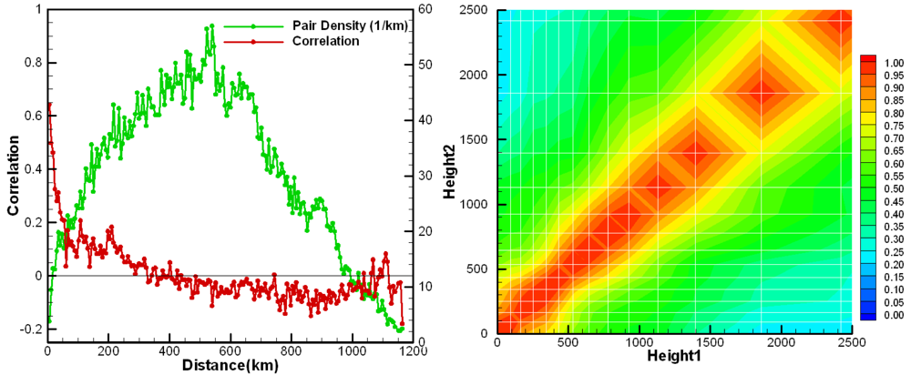
A computational grid with a 12-km resolution covering the contiguous United States (CONUS, shown in <xref ref-type="fig" rid="f1-atmosphere-02-00426">Figure 1</xref>) used in the United States National Air Quality Forecast Capability (NAQFC) is adopted here [<xref ref-type="bibr" rid="b166-atmosphere-02-00426">166</xref>]. A sub-domain covering the Mid-Atlantic region (see [<xref ref-type="bibr" rid="b29-atmosphere-02-00426">29</xref>] for detail) is used in ozone data assimilation tests and the horizontal error statistics estimation. The aerosol optical depth (AOD) assimilation tests in Section 5.3 and vertical error statistics estimation using the ozonesondes are carried out over the CONUS domain. The grid has a 22 sigma pressure hybrid vertical layers spanning from surface to 100 hPa.
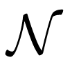
</p>
<p>Repeating the steps described in [<xref ref-type="bibr" rid="b11-atmosphere-02-00426">11</xref>], the CMAQ error statistics were estimated using the Hollingsworth-Lönnberg method. AIRNow hourly ozone observations in the sub-domain were used to calculate the horizontal error statistics.</p>
<p>Model error correlation coefficients are shown in <xref ref-type="fig" rid="f2-atmosphere-02-00426">Figure 2</xref> (left) as a function of horizontal distance between pairs of two surface stations. Pair density is also shown to indicate the number of station pairs used in the calculation. The CMAQ background model error for ozone is about 14 ppbv and its horizontal correlation length is around 50 km. Ozonesonde profiles from the measurements sites shown in <xref ref-type="fig" rid="f1-atmosphere-02-00426">Figure 1</xref> were used to calculate the vertical model error statistics shown in <xref ref-type="fig" rid="f2-atmosphere-02-00426">Figure 2</xref> (right) as a correlation coefficient contour plot.</p></sec>
<sec>
<label>5.2.</label>
<title>AIRNow Ozone Assimilation</title>
<p>Two CMAQ data assimilation systems are built with 4D-Var and OI approaches separately. The data assimilation time window is set to start from 1200Z on August 5, 2007 until 1200Z on August 6, 2007. In this 24-h period, the AIRNow hourly-averaged observations are assimilated and the observations are assumed to be un-correlated with each other and have a uniform root-mean-square error set as 3.3 ppbv. To check the effect of the data assimilation tests, an additional “forecast” day, starting from 1200Z on August 6, 2007 until 1200Z on August 7, 2007 is continuously run and will be evaluated against the AIRNow observations that are not assimilated in any of the assimilation tests.</p>
<p>In the 4D-Var data assimilation, the initial ozone concentrations are chosen as the only control parameters to be adjusted. Currently, the ozone background error covariance matrix B is assumed to be diagonal, with the root-mean-square errors set as 14.3 ppbv at every grid point. A quasi-Newton limited memory L-BFGS [<xref ref-type="bibr" rid="b167-atmosphere-02-00426">167</xref>,<xref ref-type="bibr" rid="b168-atmosphere-02-00426">168</xref>] is used in the cost functional minimization. The maximum number of iterations is set to be 15.</p>
<p>For the OI data assimilation runs, the assimilation happens every hour by combining the model results with the observations. To illustrate the effect of the background error covariance, we designed a case that eliminates the spatial correlation usage, both horizontally and vertically. It is listed in <xref ref-type="table" rid="t1-atmosphere-02-00426">Table 1</xref> as Case 3. In the other OI case, <italic>i.e</italic>., Case 4 in <xref ref-type="table" rid="t1-atmosphere-02-00426">Table 1</xref>, the horizontal background error covariance is approximated as
<disp-formula id="FD65">
<label>(38)</label>
<mml:math id="mm104" display="block">
<mml:semantics id="sm104">
<mml:mrow>
<mml:mi>B</mml:mi>
<mml:mo>=</mml:mo>
<mml:mi>H</mml:mi>
<mml:mo>⊗</mml:mo>
<mml:mi>V</mml:mi>
<mml:mo>⊗</mml:mo>
<mml:mi>C</mml:mi></mml:mrow></mml:semantics></mml:math></disp-formula></p>
<p>where <italic>H</italic> and <italic>V</italic> are matrices that represent the error correlation in horizontal and vertical directions respectively. C is the error covariance matrix at a single grid point that represents the error variances. ⊗ denotes the Kronecker product [<xref ref-type="bibr" rid="b169-atmosphere-02-00426">169</xref>]. The horizontal correlation between two grid points are calculated using a simple function 
<inline-formula>
<mml:math id="mm105" display="inline">
<mml:semantics id="sm105">
<mml:mrow>
<mml:msup>
<mml:mi>e</mml:mi>
<mml:mrow>
<mml:mo>−</mml:mo>
<mml:mfrac>
<mml:mo>Δ</mml:mo>
<mml:mrow>
<mml:msub>
<mml:mi>l</mml:mi>
<mml:mi>h</mml:mi></mml:msub></mml:mrow></mml:mfrac></mml:mrow></mml:msup></mml:mrow></mml:semantics></mml:math></inline-formula>, where Δ is the horizontal distance between the two grid pointsand <italic>l<sub>h</sub></italic> is set as 48 km. The background error variances are 14.3<sup>2</sup> ppbv<sup>2</sup>. Instead of using a constant vertical correlation structure obtained in Section 5.1, we use the boundary layer depth information available from the meteorological inputs. In Case 4, the vertical correlation coefficients are set as 1.0 for any two model grid layers inside the boundary layers. Otherwise, it is assumed there is no correlation for the background error.
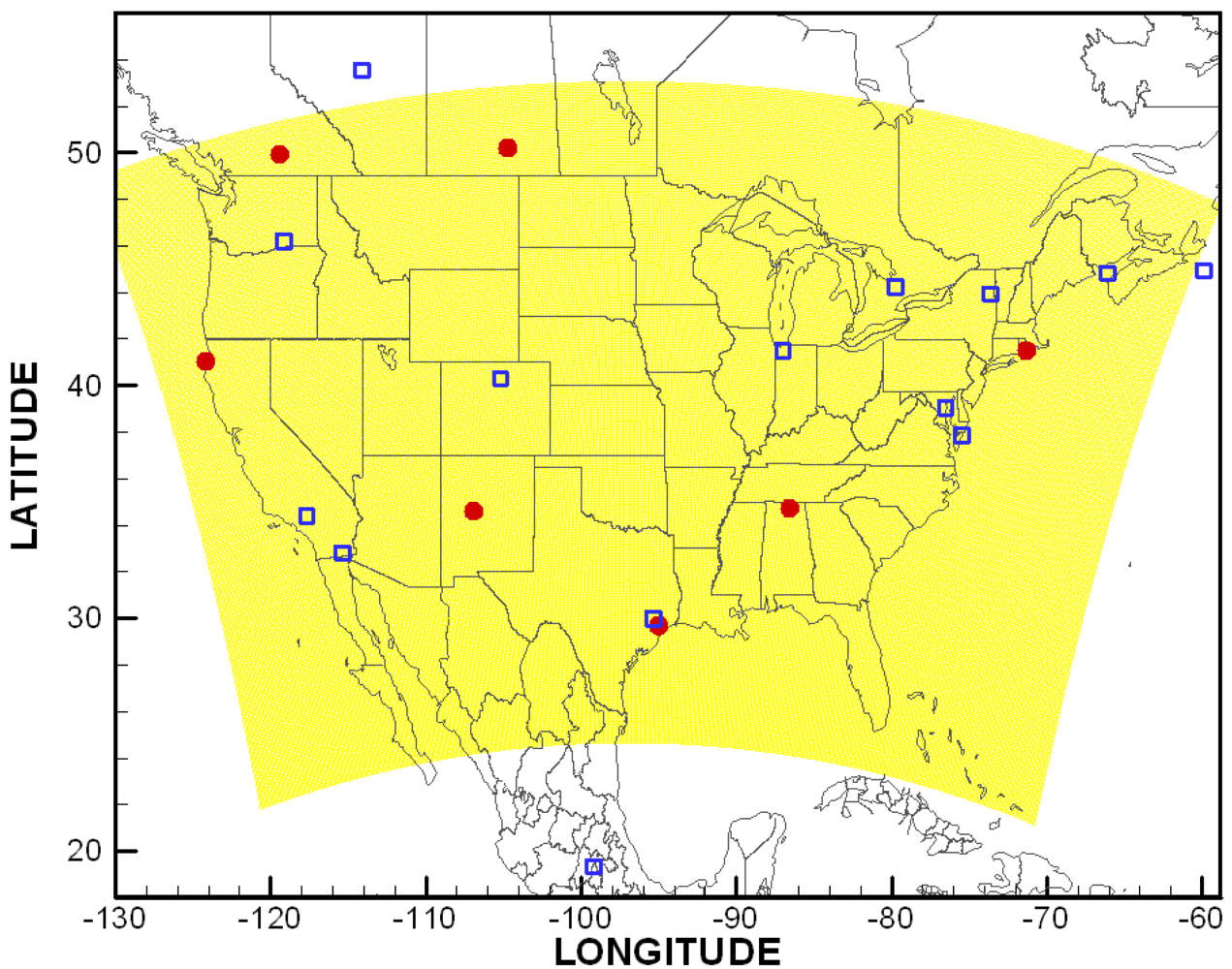
</p>
<p><xref ref-type="fig" rid="f3-atmosphere-02-00426">Figure 3</xref> shows the comparisons between the model predictions and observations of ozone during the assimilation and forecast periods for the base case and the OI case with spatial correlation accounted, <italic>i.e</italic>., Cases 1 and 4 in <xref ref-type="table" rid="t1-atmosphere-02-00426">Table 1</xref> respectively. After assimilation, the model has a much better agreement with AIRNow ozone measurements. The correlation coefficient improved from 0.59 to 0.81 during the daytime, 1300-2400Z on August 5, 2007. For the next day “forecast” run, the improvement of model ozone predictions is also apparent, with the daytime correlation coefficient between model and observations changed from 0.56 to 0.68.</p>
<p><xref ref-type="table" rid="t1-atmosphere-02-00426">Table 1</xref> lists the comparisons between the different assimilation cases and the base case run. All three assimilation cases prove to be able to generate better results not only in the assimilation day, but also in the next day “forecast”. Without fully accounting for the background error covariance, the 4D-Var case still generates the best results during the first day in terms of the model biases and root-mean-square errors (RMSEs) against the AIRNow observations. By utilizing the error statistics obtained from Section 5.1, Case 4 with the simple OI method provides the best “forecast” for the second day, where the model bias and RMSE are reduced from 8.7 ppbv to 3.1 ppbv and from 16.3 ppbv to 12.8 ppbv respectively. Without using the model background error spatial correlations, Case 3 is only slightly better than the base case for the “forecast” day. From <xref ref-type="table" rid="t1-atmosphere-02-00426">Table 1</xref>, we can see that the 4D-Var case has comparable results as Case 3, which implements the simple OI method. As indicated by the comparison between Case 3 and Case 4, replacing the diagonal background error covariance used in Case 2 with one accounting for the spatial correlation is expected to improve next day forecast for the 4D-Var case. It cannot be generalized to conclude the 4D-Var system has the same performance as OI approach. It has to be noted that the 4D-Var system is based upon CMAQ version 4.5 and the other cases implement CMAQ version 4.6.</p></sec>
<sec>
<label>5.3.</label>
<title>MODIS Aerosol Optical Depth Assimilation</title>
<p>Compared to ozone predictions, CMAQ PM2.5 predictions are much worse for the NAQFC experimental runs [<xref ref-type="bibr" rid="b170-atmosphere-02-00426">170</xref>]. MODIS AOD observations can be used to constrain the model input parameters such as emissions or initial concentrations. As a test case here, we assimilate the MODIS AOD using OI approach.</p>
<p>In the test, the MODIS AOD fine mode products are used. The model counterpart can be reconstructed by integrating the hourly extinction coefficients over the whole vertical columns. The extinction coefficients calculated from two visibility methods, Mie theory approximation and mass reconstruction method [<xref ref-type="bibr" rid="b171-atmosphere-02-00426">171</xref>], are quite similar and we chose to use the results from the mass reconstruction method. Both Terra and Aqua fine mode AOD data are used during the assimilation time period (August 14–20, 2009). Before the data assimilation tests, the AOD background error statistics is first estimated using Hollingsworth-Lönnberg approach. As an integrated quantity, only horizontal correlation is needed in constructing the error statistics. The horizontal correlation between two grid points are modeled as a function
<inline-formula>
<mml:math id="mm106" display="inline">
<mml:semantics id="sm106">
<mml:mrow>
<mml:msup>
<mml:mi>e</mml:mi>
<mml:mrow>
<mml:mo>−</mml:mo>
<mml:mfrac>
<mml:mo>Δ</mml:mo>
<mml:mrow>
<mml:msub>
<mml:mi>l</mml:mi>
<mml:mi>h</mml:mi></mml:msub></mml:mrow></mml:mfrac></mml:mrow></mml:msup></mml:mrow></mml:semantics></mml:math></inline-formula>, where <italic>l<sub>h</sub></italic> is set as 84 km. The AOD background error is assumed to be 0.6× AOD<italic><sub>MODIS</sub></italic>. In the OI assimilation, the analysis process takes place once a day, at 1700Z, which is close to the midpoint of the Terra and Aqua observation time. The adjust factor of AOD at each grid point is then uniformly applied to mass concentrations of all the aerosol species.</p>
<p><xref ref-type="fig" rid="f4-atmosphere-02-00426">Figure 4</xref> shows the AOD distributions from MODIS and CMAQ simulation with and without data assimilation. The differences after assimilation are also shown. Note that the MODIS AOD data are quite sparse, but the OI assimilation spreads the information using the obtained horizontal correlations between AOD background errors. The CMAQ PM2.5 predictions before and after AOD assimilations are evaluated using the AIRNow PM2.5 observations for each day. <xref ref-type="table" rid="t2-atmosphere-02-00426">Table 2</xref> shows the correlations between the MODIS observed and CMAQ predicted AOD before and after OI in the upper Midwest and Northeast of the U.S. (see [<xref ref-type="bibr" rid="b172-atmosphere-02-00426">172</xref>] for region definition), where most of data reside. It is seen that the <italic>R</italic><sup>2</sup> improve over four out of six days in both regions. It is encouraging as the correlation between the column quantity of AOD and the surface PM2.5 is not linear. A better reconstructed AOD cannot guarantee better predictions of surface aerosol. The current simplification of placing the observations at a single time each day and adjusting all the aerosol species using a single factor will be modified in the future. In addition, switching OI approach to 3D-Var or 4D-Var method is expected to generate better assimilation results.</p></sec></sec>
<sec sec-type="methods|conclusions">
<label>6.</label>
<title>Conclusions and Future Directions in Chemical Data Assimilation</title>
<p>New developments in chemical data assimilation techniques and algorithms, and the increased volume and diversity of available chemical measurements, have opened exciting opportunities for better science through the integration of chemical transport models and observations. Chemical data assimilation has begun to play an essential role in air quality assessments for environmental management. Widely used chemical transport models such as STEM, CMAQ, and GEOS-Chem, have been endowed with adjoint sensitivity analysis and data assimilation capabilities, and are now being used by the community to answer important scientific questions. The availability of these tools, and the growing importance of chemical weather forecasting to society, should help stimulate significant advances in chemical data assimilation in the foreseeable future.</p>
<p>Future advances will require a sustained development of new chemical data assimilation algorithms. While there is much to build upon from the assimilation experience in weather prediction, there are significant differences and challenges that are specific to chemical weather. Promising possibilities are opened up by combining the strengths of 4D-Var and EnKF techniques in hybrid data assimilation methods. Feedbacks between the meteorological and air quality components, which have mostly been studied as separate systems, are critical to improving the understanding of air quality. Future work needs to built the infrastructure required to couple meteorological and air quality forecasting and data assimilation systems. Finally, current chemical data assimilation system capabilities should be extended to enable the optimal design of the observing systems, and to rigorously quantify the informational value added by each instrument in heterogeneous sensor networks.</p></sec></body>
<back>
<sec sec-type="display-objects">
<title>Figures and Tables</title>
<fig id="f1-atmosphere-02-00426" position="float">
<label>Figure 1.</label>
<caption>
<p>CMAQ CONUS computational domain and ozonesonde locations. Red circles indicate ozonesonde locations where observations are used to calculate vertical model error statistics. Unit of longitude and latitude: degree.</p></caption>
<graphic xlink:href="atmosphere-02-00426f1.gif"/></fig>
<fig id="f2-atmosphere-02-00426" position="float">
<label>Figure 2.</label>
<caption>
<p>Ozone error statistics results through Hollingsworth-Lönnberg approach. AIRNow observations are used to get horizontal error statistics (left). Ozonesonde observations are used in calculating vertical model error statistics (right). Unit of height: meter.</p></caption>
<graphic xlink:href="atmosphere-02-00426f2.gif"/></fig>
<fig id="f3-atmosphere-02-00426" position="float">
<label>Figure 3.</label>
<caption>
<p>Scatter plots of AIRNow ozone observations and CMAQ predictions for the assimilation (upper, (<bold>a</bold>) and (<bold>b</bold>)) and hindcast (lower, (<bold>c</bold>) and (<bold>d</bold>)) period of the base (left, (a) and (c)) and OI assimilation (right, (b) and (d)) runs. (a) and (b): 1300-2400Z on August 5, 2007; (c) and (d): 1300-2400Z August 6, 2007. Correlation coefficients are 0.59, 0.81, 0.56, and 0.68 for (a), (b), (c), and (d) plots, respectively.</p></caption>
<graphic xlink:href="atmosphere-02-00426f3.gif"/></fig>
<fig id="f4-atmosphere-02-00426" position="float">
<label>Figure 4.</label>
<caption>
<p>MODIS AOD (fine mode) and CMAQ reconstructed AOD. AOD-Recona and AOD-Reconb are calculated before and after assimilation. The differences (AOD-Recona-AOD-Reconb) are also shown.</p></caption>
<graphic xlink:href="atmosphere-02-00426f4.gif"/></fig>
<table-wrap id="t1-atmosphere-02-00426" position="float">
<label>Table 1.</label>
<caption>
<p>Model ozone biases and root-mean-square errors (RMSE) against AIRNow observations during 8:00 am–8:00 pm local time on Day 1 (August 5, 2007) and Day 2 (August 6, 2007). Case 1 is the base case, <italic>i.e</italic>., without data assimilation. B: background error covariance matrix. Unit: ppbv.</p></caption>
<table frame="hsides" rules="groups">
<thead>
<tr>
<th align="left" valign="top"/>
<th align="center" valign="top"><bold>Assimilation</bold></th>
<th align="center" valign="top"><italic>B</italic></th>
<th align="center" valign="top"><bold>Day 1 Bias</bold></th>
<th align="center" valign="top"><bold>Day 1 RMSE</bold></th>
<th align="center" valign="top"><bold>Day 2 Bias</bold></th>
<th align="center" valign="top"><bold>Day 2 RMSE</bold></th></tr></thead>
<tbody>
<tr>
<td align="center" valign="top">1</td>
<td align="center" valign="top">N/A</td>
<td align="center" valign="top">8.3</td>
<td align="center" valign="top">15.9</td>
<td align="center" valign="top">8.7</td>
<td align="center" valign="top">16.3</td></tr>
<tr>
<td align="center" valign="top">2</td>
<td align="center" valign="top">4D-Var</td>
<td align="center" valign="top">Diagonal</td>
<td align="center" valign="top">−0.8</td>
<td align="center" valign="top">11.0</td>
<td align="center" valign="top">7.6</td>
<td align="center" valign="top">15.6</td></tr>
<tr>
<td align="center" valign="top">3</td>
<td align="center" valign="top">OI</td>
<td align="center" valign="top">Diagonal</td>
<td align="center" valign="top">2.6</td>
<td align="center" valign="top">12.7</td>
<td align="center" valign="top">7.5</td>
<td align="center" valign="top">15.8</td></tr>
<tr>
<td align="center" valign="top">4</td>
<td align="center" valign="top">OI</td>
<td align="center" valign="top">H⊗V⊗C</td>
<td align="center" valign="top">−1.3</td>
<td align="center" valign="top">13.2</td>
<td align="center" valign="top">3.1</td>
<td align="center" valign="top">12.8</td></tr></tbody></table></table-wrap>
<table-wrap id="t2-atmosphere-02-00426" position="float">
<label>Table 2.</label>
<caption>
<p>Correlation between CMAQ PM2.5 predictions and AIRNow hourly observations in Upper Midwest (UM) and Northeast (NE) US before and after (OI) MODIS AOD assimilation.</p></caption>
<table frame="hsides" rules="groups">
<thead>
<tr>
<th align="center" valign="top"><italic>R</italic><sup>2</sup></th>
<th align="center" valign="top"><bold>8/15/09</bold></th>
<th align="center" valign="top"><bold>8/16/09</bold></th>
<th align="center" valign="top"><bold>8/17/09</bold></th>
<th align="center" valign="top"><bold>8/18/09</bold></th>
<th align="center" valign="top"><bold>8/19/09</bold></th>
<th align="center" valign="top"><bold>8/20/09</bold></th></tr></thead>
<tbody>
<tr>
<td align="center" valign="top"><bold>UM</bold></td>
<td align="center" valign="top">0.420</td>
<td align="center" valign="top">0.138</td>
<td align="center" valign="top">0.355</td>
<td align="center" valign="top">0.154</td>
<td align="center" valign="top">0.234</td>
<td align="center" valign="top">0.021</td></tr>
<tr>
<td align="center" valign="top"><bold>UM-OI</bold></td>
<td align="center" valign="top">0.399</td>
<td align="center" valign="top">0.178</td>
<td align="center" valign="top">0.311</td>
<td align="center" valign="top">0.180</td>
<td align="center" valign="top">0.270</td>
<td align="center" valign="top">0.041</td></tr>
<tr>
<td align="center" valign="top"><bold>NE</bold></td>
<td align="center" valign="top">0.253</td>
<td align="center" valign="top">0.416</td>
<td align="center" valign="top">0.097</td>
<td align="center" valign="top">0.070</td>
<td align="center" valign="top">0.156</td>
<td align="center" valign="top">0.217</td></tr>
<tr>
<td align="center" valign="top"><bold>NE-OI</bold></td>
<td align="center" valign="top">0.306</td>
<td align="center" valign="top">0.367</td>
<td align="center" valign="top">0.110</td>
<td align="center" valign="top">0.207</td>
<td align="center" valign="top">0.171</td>
<td align="center" valign="top">0.206</td></tr></tbody></table></table-wrap></sec>
<ack>
<p>The work of A. Sandu has been supported in part by NSF through awards NSF OCI-0904397, NSF CCF-0916493, NSF DMSï£¡0915047.</p></ack>
<ref-list>
<title>References</title>
<ref id="b1-atmosphere-02-00426"><label>1.</label><citation citation-type="journal"><person-group person-group-type="author"><name><surname>Carmichael</surname><given-names>G.</given-names></name><name><surname>Chai</surname><given-names>T.</given-names></name><name><surname>Sandu</surname><given-names>A.</given-names></name><name><surname>Constantinescu</surname><given-names>E.</given-names></name><name><surname>Daescu</surname><given-names>D.</given-names></name></person-group><article-title>Predicting air quality: Improvements through advanced methods to integrate models and measurements</article-title><source>J. Comput. Phys.</source><year>2008</year><volume>227</volume><fpage>3540</fpage><lpage>3571</lpage><pub-id pub-id-type="doi">10.1016/j.jcp.2007.02.024</pub-id></citation></ref>
<ref id="b2-atmosphere-02-00426"><label>2.</label><citation citation-type="book"><person-group person-group-type="author"><name><surname>Daley</surname><given-names>R.</given-names></name></person-group><source>Atmospheric Data Analysis</source><publisher-name>Cambridge University Press</publisher-name><publisher-loc>Cambridge, UK</publisher-loc><year>1991</year></citation></ref>
<ref id="b3-atmosphere-02-00426"><label>3.</label><citation citation-type="journal"><person-group person-group-type="author"><name><surname>Courtier</surname><given-names>P.</given-names></name><name><surname>Andersson</surname><given-names>E.</given-names></name><name><surname>Heckley</surname><given-names>W.</given-names></name><name><surname>Pailleux</surname><given-names>J.</given-names></name><name><surname>Vasiljevic</surname><given-names>D.</given-names></name><name><surname>Hamrud</surname><given-names>M.</given-names></name><name><surname>Hollingsworth</surname><given-names>A.</given-names></name><name><surname>Rabier</surname><given-names>F.</given-names></name><name><surname>Fisher</surname><given-names>M.</given-names></name></person-group><article-title>The ECMWF implementation of three-dimensional variational assimilation (3D-Var)</article-title><source>Q. J. R. Meteorol. Soc.</source><comment>I: Formulation</comment><year>1998</year><volume>124</volume><fpage>1783</fpage><lpage>1807</lpage></citation></ref>
<ref id="b4-atmosphere-02-00426"><label>4.</label><citation citation-type="journal"><person-group person-group-type="author"><name><surname>Rabier</surname><given-names>F.</given-names></name><name><surname>Jarvinen</surname><given-names>H.</given-names></name><name><surname>Klinker</surname><given-names>E.</given-names></name><name><surname>Mahfouf</surname><given-names>J.</given-names></name><name><surname>Simmons</surname><given-names>A.</given-names></name></person-group><article-title>The ECMWF operational implementation of four-dimensional variational assimilation</article-title><source>Q. J. R. Meteorol. Soc.</source><comment>I: Experimental results with simplified physics</comment><year>2000</year><volume>126</volume><fpage>1148</fpage><lpage>1170</lpage></citation></ref>
<ref id="b5-atmosphere-02-00426"><label>5.</label><citation citation-type="book"><person-group person-group-type="author"><name><surname>Kalnay</surname><given-names>E.</given-names></name></person-group><source>Atmospheric Modeling, Data Assimilation and Predictability</source><publisher-name>Cambridge University Press</publisher-name><publisher-loc>Cambridge, UK</publisher-loc><year>2002</year></citation></ref>
<ref id="b6-atmosphere-02-00426"><label>6.</label><citation citation-type="book"><person-group person-group-type="author"><name><surname>Navon</surname><given-names>I.</given-names></name></person-group><source>Data assimilation for numerical weather prediction: A Review</source><publisher-name>Springer</publisher-name><publisher-loc>Berlin, Germany</publisher-loc><year>2009</year></citation></ref>
<ref id="b7-atmosphere-02-00426"><label>7.</label><citation citation-type="book"><person-group person-group-type="author"><name><surname>Evensen</surname><given-names>G.</given-names></name></person-group><source>Data Assimilation: The Ensemble Kalman Filter</source><publisher-name>Springer</publisher-name><publisher-loc>Berlin, Germany</publisher-loc><year>2007</year></citation></ref>
<ref id="b8-atmosphere-02-00426"><label>8.</label><citation citation-type="journal"><person-group person-group-type="author"><name><surname>Chai</surname><given-names>T.</given-names></name><name><surname>Carmichael</surname><given-names>G.</given-names></name><name><surname>Sandu</surname><given-names>A.</given-names></name><name><surname>Tang</surname><given-names>Y.</given-names></name><name><surname>Daescu</surname><given-names>D.</given-names></name></person-group><article-title>Chemical data assimilation with TRACE-P aircraft measurements</article-title><source>J. Geophys. Res.</source><year>2006</year><volume>111</volume><fpage>D02301</fpage><pub-id pub-id-type="doi">10.1029/2005JD005883</pub-id></citation></ref>
<ref id="b9-atmosphere-02-00426"><label>9.</label><citation citation-type="journal"><person-group person-group-type="author"><name><surname>Hakami</surname><given-names>A.</given-names></name><name><surname>Seinfeld</surname><given-names>J.</given-names></name><name><surname>Chai</surname><given-names>T.</given-names></name><name><surname>Tang</surname><given-names>Y.</given-names></name><name><surname>Carmichael</surname><given-names>G.</given-names></name><name><surname>Sandu</surname><given-names>A.</given-names></name></person-group><article-title>Adjoint sensitivity analysis of ozone non-attainment over the continental United States</article-title><source>Environ. Sci. Technol.</source><year>2006</year><volume>40</volume><fpage>3855</fpage><lpage>3864</lpage><pub-id pub-id-type="doi">10.1021/es052135g</pub-id><pub-id pub-id-type="pmid">16830553</pub-id></citation></ref>
<ref id="b10-atmosphere-02-00426"><label>10.</label><citation citation-type="journal"><person-group person-group-type="author"><name><surname>Zhang</surname><given-names>L.</given-names></name><name><surname>Sandu</surname><given-names>A.</given-names></name></person-group><article-title>Data assimilation in multiscale chemical transport models</article-title><source>LNCS</source><year>2007</year><volume>4487</volume><fpage>1026</fpage><lpage>1033</lpage></citation></ref>
<ref id="b11-atmosphere-02-00426"><label>11.</label><citation citation-type="journal"><person-group person-group-type="author"><name><surname>Chai</surname><given-names>T.</given-names></name><name><surname>Carmichael</surname><given-names>G.</given-names></name><name><surname>Tang</surname><given-names>Y.</given-names></name><name><surname>Sandu</surname><given-names>A.</given-names></name><name><surname>Hardesty</surname><given-names>M.</given-names></name><name><surname>Pilewskie</surname><given-names>P.</given-names></name><name><surname>Whitlow</surname><given-names>S.</given-names></name><name><surname>Browell</surname><given-names>E.</given-names></name><name><surname>Avery</surname><given-names>M.</given-names></name><name><surname>Thouret</surname><given-names>V.</given-names></name><etal/></person-group><article-title>Four dimensional data assimilation experiments with ICARTT (international consortium for atmospheric transport and transformation) ozone measurements</article-title><source>J. Geophys. Res.</source><year>2007</year><volume>112</volume><fpage>D12S15</fpage><pub-id pub-id-type="doi">10.1029/2006JD007763</pub-id></citation></ref>
<ref id="b12-atmosphere-02-00426"><label>12.</label><citation citation-type="journal"><person-group person-group-type="author"><name><surname>Zhang</surname><given-names>L.</given-names></name><name><surname>Constantinescu</surname><given-names>E.</given-names></name><name><surname>Sandu</surname><given-names>A.</given-names></name><name><surname>Tang</surname><given-names>Y.</given-names></name><name><surname>Chai</surname><given-names>T.</given-names></name><name><surname>Carmichael</surname><given-names>G.</given-names></name><name><surname>Byun</surname><given-names>D.</given-names></name><name><surname>Olaguer</surname><given-names>E.</given-names></name></person-group><article-title>An adjoint sensitivity analysis and 4D-Var data assimilation study of Texas air quality</article-title><source>Atmos. Environ.</source><year>2008</year><volume>42</volume><fpage>5787</fpage><lpage>5804</lpage><pub-id pub-id-type="doi">10.1016/j.atmosenv.2008.03.048</pub-id></citation></ref>
<ref id="b13-atmosphere-02-00426"><label>13.</label><citation citation-type="journal"><person-group person-group-type="author"><name><surname>Singh</surname><given-names>K.</given-names></name><name><surname>Eller</surname><given-names>P.</given-names></name><name><surname>Sandu</surname><given-names>A.</given-names></name><name><surname>Bowman</surname><given-names>K.</given-names></name><name><surname>Jones</surname><given-names>D.</given-names></name><name><surname>Lee</surname><given-names>M.</given-names></name></person-group><article-title>Improving GEOS-chem model forecasts through profile retrievals from tropospheric emission spectrometer</article-title><source>LNCS</source><year>2009</year><volume>5545</volume><fpage>302</fpage><lpage>311</lpage></citation></ref>
<ref id="b14-atmosphere-02-00426"><label>14.</label><citation citation-type="journal"><person-group person-group-type="author"><name><surname>Gou</surname><given-names>T.</given-names></name><name><surname>Singh</surname><given-names>K.</given-names></name><name><surname>Sandu</surname><given-names>A.</given-names></name></person-group><article-title>Chemical data assimilation with CMAQ: Continuous vs. discrete advection adjoints</article-title><source>LNCS</source><year>2009</year><volume>5545</volume><fpage>312</fpage><lpage>321</lpage></citation></ref>
<ref id="b15-atmosphere-02-00426"><label>15.</label><citation citation-type="journal"><person-group person-group-type="author"><name><surname>Chai</surname><given-names>T.</given-names></name><name><surname>Carmichael</surname><given-names>G.</given-names></name><name><surname>Tang</surname><given-names>Y.</given-names></name><name><surname>Sandu</surname><given-names>A.</given-names></name></person-group><article-title>Regional <italic>NO<sub>X</sub></italic> emission inversion through a four-dimensional variational approach using SCIAMACHY tropospheric <italic>NO</italic><sub>2</sub> column observations</article-title><source>Atmos. Environ.</source><year>2009</year><volume>43</volume><fpage>5046</fpage><lpage>5055</lpage><pub-id pub-id-type="doi">10.1016/j.atmosenv.2009.06.052</pub-id></citation></ref>
<ref id="b16-atmosphere-02-00426"><label>16.</label><citation citation-type="journal"><person-group person-group-type="author"><name><surname>Gou</surname><given-names>T.</given-names></name><name><surname>Sandu</surname><given-names>A.</given-names></name></person-group><article-title>Continuous <italic>versus</italic> discrete advection adjoints in chemical data assimilation with CMAQ</article-title><source>Atmos. Environ.</source><year>2011</year><volume>45</volume><fpage>4868</fpage><lpage>4881</lpage><pub-id pub-id-type="doi">10.1016/j.atmosenv.2011.06.015</pub-id></citation></ref>
<ref id="b17-atmosphere-02-00426"><label>17.</label><citation citation-type="journal"><person-group person-group-type="author"><name><surname>Singh</surname><given-names>K.</given-names></name><name><surname>Sandu</surname><given-names>A.</given-names></name><name><surname>Parrington</surname><given-names>M.</given-names></name><name><surname>Jones</surname><given-names>D.</given-names></name><name><surname>Bowman</surname><given-names>K.</given-names></name><name><surname>Lee</surname><given-names>M.</given-names></name></person-group><article-title>Ozone data assimilation with GEOS-Chem: A comparison between 3D-Var, 4D-Var, and suboptimal Kalman filter approaches</article-title><comment>Unpublished work</comment><year>2011</year><pub-id pub-id-type="doi">10.1016/j.atmosenv.2011.06.015</pub-id></citation></ref>
<ref id="b18-atmosphere-02-00426"><label>18.</label><citation citation-type="confproc"><person-group person-group-type="author"><name><surname>Alexe</surname><given-names>M.</given-names></name><name><surname>Sandu</surname><given-names>A.</given-names></name></person-group><article-title>Adaptive Solution of Time-Dependent Inverse Problems with the Discrete Adjoint Method</article-title><conf-name>Proceedigns of the International Conference on Computational Science (ICCS-2011)</conf-name><conf-loc>Bali, Indonesia</conf-loc><conf-date>26-28 October 2011</conf-date><comment>in press</comment></citation></ref>
<ref id="b19-atmosphere-02-00426"><label>19.</label><citation citation-type="journal"><person-group person-group-type="author"><name><surname>Stewart</surname><given-names>R.</given-names></name></person-group><article-title>Multiple steady states in atmospheric chemistry</article-title><source>J. Geophys. Res.</source><year>1993</year><volume>98</volume><fpage>20601</fpage><lpage>20612</lpage><pub-id pub-id-type="doi">10.1029/93JD02408</pub-id></citation></ref>
<ref id="b20-atmosphere-02-00426"><label>20.</label><citation citation-type="journal"><person-group person-group-type="author"><name><surname>Menut</surname><given-names>L.</given-names></name></person-group><article-title>Adjoint modeling for atmospheric pollution process sensitivity at regional scale</article-title><source>J. Geophys. Res.</source><year>2003</year><volume>108</volume></citation></ref>
<ref id="b21-atmosphere-02-00426"><label>21.</label><citation citation-type="journal"><person-group person-group-type="author"><name><surname>Dee</surname><given-names>D.</given-names></name><name><surname>da Silva</surname><given-names>A.</given-names></name></person-group><article-title>Data assimilation in the presence of forecast bias</article-title><source>Q. J. R. Meteorol. Soc.</source><year>1998</year><volume>124</volume><fpage>269</fpage><lpage>295</lpage><pub-id pub-id-type="doi">10.1002/qj.49712454512</pub-id></citation></ref>
<ref id="b22-atmosphere-02-00426"><label>22.</label><citation citation-type="journal"><person-group person-group-type="author"><name><surname>Van der A</surname><given-names>R.J.</given-names></name><name><surname>Allaart</surname><given-names>M.A.F.</given-names></name><name><surname>Eskes</surname><given-names>H.J.</given-names></name></person-group><article-title>Multi sensor reanalysis of total ozone</article-title><source>Atmos Chem. Phys.</source><year>2010</year><volume>10</volume><fpage>11277</fpage><lpage>11294</lpage><pub-id pub-id-type="doi">10.5194/acp-10-11277-2010</pub-id></citation></ref>
<ref id="b23-atmosphere-02-00426"><label>23.</label><citation citation-type="book"><person-group person-group-type="author"><name><surname>Evans</surname><given-names>L.</given-names></name></person-group><source>Partial Differential Equations</source><publisher-name>Americal Mathematical Society</publisher-name><publisher-loc>Providence, RI, USA</publisher-loc><year>1998</year></citation></ref>
<ref id="b24-atmosphere-02-00426"><label>24.</label><citation citation-type="web"><person-group person-group-type="author"><collab>Community Modeling and Analysis System (CMAS)</collab></person-group><comment>Available online: <ext-link xlink:href="http://www.cmascenter.org" ext-link-type="uri">http://www.cmascenter.org</ext-link> (accessed on 2 May 2011)</comment></citation></ref>
<ref id="b25-atmosphere-02-00426"><label>25.</label><citation citation-type="journal"><person-group person-group-type="author"><name><surname>Byun</surname><given-names>D.</given-names></name></person-group><article-title>Dynamically consistent formulations in meteorological and air quality models for multiscale atmospheric studies part I: Governing equations in a generalized coordinate system</article-title><source>J. Atmos. Sci.</source><year>1999</year><volume>56</volume><fpage>3789</fpage><lpage>3807</lpage><pub-id pub-id-type="doi">10.1175/1520-0469(1999)056&lt;3789:DCFIMA&gt;2.0.CO;2</pub-id></citation></ref>
<ref id="b26-atmosphere-02-00426"><label>26.</label><citation citation-type="journal"><person-group person-group-type="author"><name><surname>Byun</surname><given-names>D.</given-names></name></person-group><article-title>Dynamically consistent formulations in meteorological and air quality models for multiscale atmospheric studies part II: Mass conservation issues</article-title><source>J. Atmos. Sci.</source><year>1999</year><volume>56</volume><fpage>3808</fpage><lpage>3820</lpage><pub-id pub-id-type="doi">10.1175/1520-0469(1999)056&lt;3808:DCFIMA&gt;2.0.CO;2</pub-id></citation></ref>
<ref id="b27-atmosphere-02-00426"><label>27.</label><citation citation-type="journal"><person-group person-group-type="author"><name><surname>Hakami</surname><given-names>A.</given-names></name><name><surname>Henze</surname><given-names>D.</given-names></name><name><surname>Seinfeld</surname><given-names>J.</given-names></name><name><surname>Singh</surname><given-names>K.</given-names></name><name><surname>Sandu</surname><given-names>A.</given-names></name><name><surname>Kim</surname><given-names>S.</given-names></name><name><surname>Byun</surname><given-names>D.</given-names></name><name><surname>Li</surname><given-names>Q.</given-names></name></person-group><article-title>The adjoint of CMAQ</article-title><source>Environ. Sci. Technol.</source><year>2007</year><volume>41</volume><fpage>7807</fpage><lpage>7817</lpage><pub-id pub-id-type="doi">10.1021/es070944p</pub-id><pub-id pub-id-type="pmid">18075092</pub-id></citation></ref>
<ref id="b28-atmosphere-02-00426"><label>28.</label><citation citation-type="web"><article-title>The AIRNow network</article-title><comment>Available online: <ext-link xlink:href="http://airnow.gov" ext-link-type="uri">http://airnow.gov</ext-link> (accessed on 2 May 2011)</comment></citation></ref>
<ref id="b29-atmosphere-02-00426"><label>29.</label><citation citation-type="book"><person-group person-group-type="author"><name><surname>Sandu</surname><given-names>A.</given-names></name><name><surname>Chai</surname><given-names>T.</given-names></name><name><surname>Carmichael</surname><given-names>G.</given-names></name></person-group><article-title>Integration of models and observations: A modern paradigm for air quality</article-title><source>Modelling of Pollutants in Complex Environments</source><person-group person-group-type="editor"><name><surname>Hanrahan</surname><given-names>G.</given-names></name></person-group><publisher-name>ILM Publications</publisher-name><publisher-loc>St Albans, UK</publisher-loc><year>2010</year><volume>2</volume><fpage>419</fpage><lpage>434</lpage><comment>Chapter 15</comment></citation></ref>
<ref id="b30-atmosphere-02-00426"><label>30.</label><citation citation-type="journal"><person-group person-group-type="author"><name><surname>Zubrow</surname><given-names>A.</given-names></name><name><surname>Chen</surname><given-names>L.</given-names></name><name><surname>Kotamarthi</surname><given-names>V.</given-names></name></person-group><article-title>EAKF-CMAQ: Introduction and evaluation of a data assimilation for CMAQ based on the ensemble adjustment Kalman filter</article-title><source>J. Geophys. Res.</source><year>2008</year><volume>113</volume><fpage>D09302</fpage><pub-id pub-id-type="doi">10.1029/2007JD009267</pub-id></citation></ref>
<ref id="b31-atmosphere-02-00426"><label>31.</label><citation citation-type="journal"><person-group person-group-type="author"><name><surname>Jeuken</surname><given-names>A.</given-names></name><name><surname>Eskes</surname><given-names>H.</given-names></name><name><surname>van Velthoven</surname><given-names>P.</given-names></name><name><surname>Kelder</surname><given-names>H.</given-names></name><name><surname>Holm</surname><given-names>E.</given-names></name></person-group><article-title>Assimilation of total ozone satellite measurements in a three-dimensional tracer transport model</article-title><source>J. Geophys. Res.</source><year>1999</year><volume>104</volume><fpage>5551</fpage><lpage>5563</lpage><pub-id pub-id-type="doi">10.1029/1998JD100052</pub-id></citation></ref>
<ref id="b32-atmosphere-02-00426"><label>32.</label><citation citation-type="journal"><person-group person-group-type="author"><name><surname>Thompson</surname><given-names>A.</given-names></name><name><surname>Witte</surname><given-names>J.</given-names></name><name><surname>McPeters</surname><given-names>R.</given-names></name><name><surname>Oltmans</surname><given-names>S.</given-names></name><name><surname>Schmidlin</surname><given-names>F.</given-names></name><name><surname>Logan</surname><given-names>J.</given-names></name><name><surname>Fujiwara</surname><given-names>M.</given-names></name><name><surname>Kirchhoff</surname><given-names>V.</given-names></name><name><surname>Posny</surname><given-names>F.</given-names></name><name><surname>Coetzee</surname><given-names>G.</given-names></name><etal/></person-group><article-title>Southern hemisphere additional ozonesondes (SHADOZ) 1998-2000 tropical ozone climatology—1</article-title><comment>Comparison with total ozone mapping spectrometer (TOMS) and ground-based measurements</comment><source>J. Geophys. Res.</source><year>2003</year><volume>108</volume><fpage>8238</fpage><pub-id pub-id-type="doi">10.1029/2001JD000967</pub-id></citation></ref>
<ref id="b33-atmosphere-02-00426"><label>33.</label><citation citation-type="journal"><person-group person-group-type="author"><name><surname>Thompson</surname><given-names>A.</given-names></name><name><surname>Witte</surname><given-names>J.</given-names></name><name><surname>Schmidlin</surname><given-names>F.</given-names></name><name><surname>Logan</surname><given-names>J.</given-names></name><name><surname>Fujiwara</surname><given-names>M.</given-names></name><name><surname>Kirchhoff</surname><given-names>V.</given-names></name><name><surname>Posny</surname><given-names>F.</given-names></name><name><surname>Coetzee</surname><given-names>G.</given-names></name><name><surname>Hoegger</surname><given-names>B.</given-names></name><name><surname>Kawakami</surname><given-names>S.</given-names></name><etal/></person-group><article-title>Southern hemisphere additional ozonesondes (SHADOZ) 1998-2000 tropical ozone climatology—2</article-title><comment>Tropospheric variability and the zonal wave-one</comment><source>J. Geophys. Res.</source><year>2003</year><volume>108</volume><fpage>8241</fpage><pub-id pub-id-type="doi">10.1029/2002JD002241</pub-id></citation></ref>
<ref id="b34-atmosphere-02-00426"><label>34.</label><citation citation-type="journal"><person-group person-group-type="author"><name><surname>Thompson</surname><given-names>A.</given-names></name><name><surname>Witte</surname><given-names>J.</given-names></name><name><surname>Smit</surname><given-names>H.</given-names></name><name><surname>Oltmans</surname><given-names>S.</given-names></name><name><surname>Johnson</surname><given-names>B.</given-names></name><name><surname>Kirchhoff</surname><given-names>V.</given-names></name><name><surname>Schmidlin</surname><given-names>F.</given-names></name></person-group><article-title>Southern hemisphere additional ozonesondes (SHADOZ) 1998-2000 tropical ozone climatology—3</article-title><comment>Instrumentation, station-to-station variability, and evaluation with simulated flight profiles</comment><source>J. Geophys. Res.</source><year>2007</year><volume>112</volume><fpage>D03304</fpage><pub-id pub-id-type="doi">10.1029/2005JD007042</pub-id></citation></ref>
<ref id="b35-atmosphere-02-00426"><label>35.</label><citation citation-type="web"><person-group person-group-type="author"><collab>Japan National Institute for Environmental Studies (NIES) lidars</collab></person-group><comment>Available online: <ext-link xlink:href="http://www-lidar.nies.go.jp" ext-link-type="uri">http://www-lidar.nies.go.jp</ext-link> (accessed on 2 May 2011)</comment></citation></ref>
<ref id="b36-atmosphere-02-00426"><label>36.</label><citation citation-type="journal"><person-group person-group-type="author"><name><surname>Yumimoto</surname><given-names>K.</given-names></name><name><surname>Uno</surname><given-names>I.</given-names></name><name><surname>Sugimoto</surname><given-names>N.</given-names></name><name><surname>Shimizu</surname><given-names>A.</given-names></name><name><surname>Liu</surname><given-names>Z.</given-names></name><name><surname>Winker</surname><given-names>D.</given-names></name></person-group><article-title>Adjoint inversion modeling of Asian dust emission using lidar observations</article-title><source>Atmos. Chem. Phys.</source><year>2008</year><volume>8</volume><fpage>2869</fpage><lpage>2884</lpage><pub-id pub-id-type="doi">10.5194/acp-8-2869-2008</pub-id></citation></ref>
<ref id="b37-atmosphere-02-00426"><label>37.</label><citation citation-type="journal"><person-group person-group-type="author"><name><surname>Fishman</surname><given-names>J.</given-names></name><name><surname>Bowman</surname><given-names>K.W.</given-names></name><name><surname>Burrows</surname><given-names>J.P.</given-names></name><name><surname>Richter</surname><given-names>A.</given-names></name><name><surname>Chance</surname><given-names>K.V.</given-names></name><name><surname>Edwards</surname><given-names>D.P.</given-names></name><name><surname>Martin</surname><given-names>R.V.</given-names></name><name><surname>Morris</surname><given-names>G.A.</given-names></name><name><surname>Pierce</surname><given-names>R.B.</given-names></name><name><surname>Ziemke</surname><given-names>J.R.</given-names></name><etal/></person-group><article-title>Remote sensing of tropospheric pollution from space</article-title><source>Bull. Am. Meteorol. Soc.</source><year>2008</year><volume>89</volume><fpage>805</fpage><lpage>821</lpage><pub-id pub-id-type="doi">10.1175/2008BAMS2526.1</pub-id></citation></ref>
<ref id="b38-atmosphere-02-00426"><label>38.</label><citation citation-type="journal"><person-group person-group-type="author"><name><surname>Martin</surname><given-names>R.V.</given-names></name></person-group><article-title>Satellite remote sensing of surface air quality</article-title><source>Atmos. Environ.</source><year>2008</year><volume>42</volume><fpage>7823</fpage><lpage>7843</lpage><pub-id pub-id-type="doi">10.1016/j.atmosenv.2008.07.018</pub-id></citation></ref>
<ref id="b39-atmosphere-02-00426"><label>39.</label><citation citation-type="web"><person-group person-group-type="author"><collab>Aura satellite</collab></person-group><comment>Available online: <ext-link xlink:href="http://aura.gsfc.nasa.gov/index.html" ext-link-type="uri">http://aura.gsfc.nasa.gov/index.html</ext-link> (accessed on 2 May 2011)</comment></citation></ref>
<ref id="b40-atmosphere-02-00426"><label>40.</label><citation citation-type="journal"><person-group person-group-type="author"><name><surname>Schoeberl</surname><given-names>M.</given-names></name><name><surname>Douglass</surname><given-names>A.</given-names></name><name><surname>Hilsenrath</surname><given-names>E.</given-names></name><name><surname>Bhartia</surname><given-names>P.</given-names></name><name><surname>Beer</surname><given-names>R.</given-names></name><name><surname>Waters</surname><given-names>J.</given-names></name><name><surname>Gunson</surname><given-names>M.</given-names></name><name><surname>Froidevaux</surname><given-names>L.</given-names></name><name><surname>Gille</surname><given-names>J.</given-names></name><name><surname>Barnett</surname><given-names>J.</given-names></name><etal/></person-group><article-title>Overview of the EOS aura mission</article-title><source>IEEE Trans. Geosci. Remote Sens.</source><year>2006</year><volume>44</volume><fpage>1066</fpage><lpage>1074</lpage><pub-id pub-id-type="doi">10.1109/TGRS.2005.861950</pub-id></citation></ref>
<ref id="b41-atmosphere-02-00426"><label>41.</label><citation citation-type="journal"><person-group person-group-type="author"><name><surname>Bovensmann</surname><given-names>H.</given-names></name><name><surname>Burrows</surname><given-names>J.P.</given-names></name><name><surname>Buchwitz</surname><given-names>M.</given-names></name><name><surname>Frerick</surname><given-names>J.</given-names></name><name><surname>Noël</surname><given-names>S.</given-names></name><name><surname>Rozanov</surname><given-names>V.V.</given-names></name></person-group><article-title>SCIAMACHY: Mission objectives and measurement modes</article-title><source>J. Atmos. Sci.</source><year>1999</year><volume>56</volume><fpage>127</fpage><lpage>150</lpage><pub-id pub-id-type="doi">10.1175/1520-0469(1999)056&lt;0127:SMOAMM&gt;2.0.CO;2</pub-id></citation></ref>
<ref id="b42-atmosphere-02-00426"><label>42.</label><citation citation-type="journal"><person-group person-group-type="author"><name><surname>Kaufman</surname><given-names>Y.</given-names></name><name><surname>Tanre</surname><given-names>D.</given-names></name><name><surname>Remer</surname><given-names>L.</given-names></name><name><surname>Vermote</surname><given-names>E.</given-names></name><name><surname>Chu</surname><given-names>A.</given-names></name><name><surname>Holben</surname><given-names>B.</given-names></name></person-group><article-title>Applications of the quasi-inverse method to data assimilation</article-title><source>J. Geophys. Res.</source><year>1997</year><volume>102</volume><fpage>17051</fpage><lpage>17067</lpage><pub-id pub-id-type="doi">10.1029/96JD03988</pub-id></citation></ref>
<ref id="b43-atmosphere-02-00426"><label>43.</label><citation citation-type="journal"><person-group person-group-type="author"><name><surname>Remer</surname><given-names>L.</given-names></name><name><surname>Kaufman</surname><given-names>Y.</given-names></name><name><surname>Tanre</surname><given-names>D.</given-names></name><name><surname>Mattoo</surname><given-names>S.</given-names></name><name><surname>Chu</surname><given-names>D.</given-names></name><name><surname>Martins</surname><given-names>J.</given-names></name><name><surname>Li</surname><given-names>R.R.</given-names></name><name><surname>Ichoku</surname><given-names>C.</given-names></name><name><surname>Levy</surname><given-names>R.</given-names></name><name><surname>Kleidman</surname><given-names>R.</given-names></name><etal/></person-group><article-title>The MODIS aerosol algorithm, products, and validation</article-title><source>J. Atmos. Sci.</source><year>2005</year><volume>62</volume><fpage>947</fpage><lpage>973</lpage><pub-id pub-id-type="doi">10.1175/JAS3385.1</pub-id></citation></ref>
<ref id="b44-atmosphere-02-00426"><label>44.</label><citation citation-type="journal"><person-group person-group-type="author"><name><surname>Matsui</surname><given-names>T.</given-names></name><name><surname>Kreidenweis</surname><given-names>S.</given-names></name><name><surname>Pielke</surname><given-names>R.</given-names></name><name><surname>Schichtel</surname><given-names>B.</given-names></name><name><surname>Yu</surname><given-names>H.</given-names></name><name><surname>Chin</surname><given-names>M.</given-names></name><name><surname>Chu</surname><given-names>D.</given-names></name><name><surname>Niyogi</surname><given-names>D.</given-names></name></person-group><article-title>Regional comparison and assimilation of GOCART and MODIS aerosol optical depth across the eastern US</article-title><source>Geophys. Res. Lett.</source><year>2004</year><volume>31</volume><fpage>L21101</fpage><pub-id pub-id-type="doi">10.1029/2004GL021017</pub-id></citation></ref>
<ref id="b45-atmosphere-02-00426"><label>45.</label><citation citation-type="journal"><person-group person-group-type="author"><name><surname>Adhikary</surname><given-names>B.</given-names></name><name><surname>Kulkarni</surname><given-names>S.</given-names></name><name><surname>Dallura</surname><given-names>A.</given-names></name><name><surname>Tang</surname><given-names>Y.</given-names></name><name><surname>Chai</surname><given-names>T.</given-names></name><name><surname>Leung</surname><given-names>L.</given-names></name><name><surname>Qian</surname><given-names>Y.</given-names></name><name><surname>Chung</surname><given-names>C.</given-names></name><name><surname>Ramanathan</surname><given-names>V.</given-names></name><name><surname>Carmichael</surname><given-names>G.</given-names></name></person-group><article-title>A regional scale chemical transport modeling of Asian aerosols with data assimilation of AOD observations using optimal interpolation technique</article-title><source>Atmos. Environ.</source><year>2008</year><volume>42</volume><fpage>8600</fpage><lpage>8615</lpage><pub-id pub-id-type="doi">10.1016/j.atmosenv.2008.08.031</pub-id></citation></ref>
<ref id="b46-atmosphere-02-00426"><label>46.</label><citation citation-type="journal"><person-group person-group-type="author"><name><surname>Zhang</surname><given-names>J.</given-names></name><name><surname>Reid</surname><given-names>J.S.</given-names></name><name><surname>Westphal</surname><given-names>D.L.</given-names></name><name><surname>Baker</surname><given-names>N.L.</given-names></name><name><surname>Hyer</surname><given-names>E.J.</given-names></name></person-group><article-title>A system for operational aerosol optical depth data assimilation over global oceans</article-title><source>J. Geophys. Res.</source><year>2008</year><volume>113</volume><fpage>D10208</fpage><pub-id pub-id-type="doi">10.1029/2007JD009065</pub-id></citation></ref>
<ref id="b47-atmosphere-02-00426"><label>47.</label><citation citation-type="journal"><person-group person-group-type="author"><name><surname>Benedetti</surname><given-names>A.</given-names></name><name><surname>Morcrette</surname><given-names>J.J.</given-names></name><name><surname>Boucher</surname><given-names>O.</given-names></name><name><surname>Dethof</surname><given-names>A.</given-names></name><name><surname>Engelen</surname><given-names>R.J.</given-names></name><name><surname>Fisher</surname><given-names>M.</given-names></name><name><surname>Flentje</surname><given-names>H.</given-names></name><name><surname>Huneeus</surname><given-names>N.</given-names></name><name><surname>Jones</surname><given-names>L.</given-names></name><name><surname>Kaiser</surname><given-names>J.W.</given-names></name><etal/></person-group><article-title>Aerosol analysis and forecast in the European Centre for medium-range weather forecasts integrated forecast system: 2. Data assimilation</article-title><source>J. Geophys. Res.</source><year>2009</year><volume>114</volume><fpage>D13205</fpage><pub-id pub-id-type="doi">10.1029/2008JD011115</pub-id></citation></ref>
<ref id="b48-atmosphere-02-00426"><label>48.</label><citation citation-type="journal"><person-group person-group-type="author"><name><surname>Štajner</surname><given-names>I.</given-names></name><name><surname>Riishøjgaard</surname><given-names>L.P.</given-names></name><name><surname>Rood</surname><given-names>R.B.</given-names></name></person-group><article-title>The GEOS ozone data assimilation system: Specification of error statistics</article-title><source>Q. J. R. Meteorol. Soc.</source><year>2001</year><volume>127</volume><fpage>1069</fpage><lpage>1094</lpage><pub-id pub-id-type="doi">10.1002/qj.49712757320</pub-id></citation></ref>
<ref id="b49-atmosphere-02-00426"><label>49.</label><citation citation-type="journal"><person-group person-group-type="author"><name><surname>Nassar</surname><given-names>R.</given-names></name><name><surname>Jones</surname><given-names>D.</given-names></name><name><surname>Kulawik</surname><given-names>S.</given-names></name><name><surname>Worden</surname><given-names>J.</given-names></name><name><surname>Bowman</surname><given-names>K.</given-names></name><name><surname>Andres</surname><given-names>R.</given-names></name><name><surname>Suntharalingam</surname><given-names>P.</given-names></name><name><surname>Chen</surname><given-names>J.</given-names></name><name><surname>Brenninkmeijer</surname><given-names>C.</given-names></name><name><surname>Schuck</surname><given-names>T.</given-names></name><etal/></person-group><article-title>Inverse modeling of <italic>CO</italic><sub>2</sub> sources and sinks using satellite observations of <italic>CO</italic><sub>2</sub> from TES and surface flask measurements</article-title><source>Atmos. Chem. Phys.</source><year>2011</year><volume>11</volume><fpage>6029</fpage><lpage>6047</lpage><pub-id pub-id-type="doi">10.5194/acp-11-6029-2011</pub-id></citation></ref>
<ref id="b50-atmosphere-02-00426"><label>50.</label><citation citation-type="journal"><person-group person-group-type="author"><name><surname>Fehsenfeld</surname><given-names>F.C.</given-names></name><name><surname>Ancellet</surname><given-names>G.</given-names></name><name><surname>Bates</surname><given-names>T.S.</given-names></name><name><surname>Goldstein</surname><given-names>A.H.</given-names></name><name><surname>Hardesty</surname><given-names>R.M.</given-names></name><name><surname>Honrath</surname><given-names>R.</given-names></name><name><surname>Law</surname><given-names>K.S.</given-names></name><name><surname>Lewis</surname><given-names>A.C.</given-names></name><name><surname>Leaitch</surname><given-names>R.</given-names></name><name><surname>McKeen</surname><given-names>S.</given-names></name><etal/></person-group><article-title>International consortium for atmospheric research on transport and transformation (ICARTT): North America to Europe-overview of the 2004 summer field study</article-title><source>J. Geophys. Res.</source><year>2006</year><volume>111</volume><fpage>D23S01</fpage><pub-id pub-id-type="doi">10.1029/2006JD007829</pub-id></citation></ref>
<ref id="b51-atmosphere-02-00426"><label>51.</label><citation citation-type="web"><person-group person-group-type="author"><collab>New England Air Quality Study - Intercontinental Transport and Chemical Transformation (NEAQS-ITCT)</collab></person-group><comment>Available online: <ext-link xlink:href="http://saga.pmel.noaa.gov/Field/NEAQS-ITCT" ext-link-type="uri">http://saga.pmel.noaa.gov/Field/NEAQS-ITCT</ext-link> (accessed on 2 May 2011)</comment></citation></ref>
<ref id="b52-atmosphere-02-00426"><label>52.</label><citation citation-type="journal"><person-group person-group-type="author"><name><surname>Gustafson</surname><given-names>W.</given-names></name><name><surname>Chapman</surname><given-names>E.</given-names></name><name><surname>Ghan</surname><given-names>S.</given-names></name><name><surname>Easter</surname><given-names>RC</given-names></name><name><surname>Fast</surname><given-names>J.</given-names></name></person-group><article-title>Impact on modeled cloud characteristics due to simplified treatment of uniform cloud condensation nuclei during NEAQS 2004</article-title><source>Geophys. Res. Lett.</source><year>2007</year><volume>34</volume><fpage>1</fpage><lpage>5</lpage></citation></ref>
<ref id="b53-atmosphere-02-00426"><label>53.</label><citation citation-type="journal"><person-group person-group-type="author"><name><surname>Ravetta</surname><given-names>F.</given-names></name><name><surname>Ancellet</surname><given-names>G.</given-names></name><name><surname>Colette</surname><given-names>A.</given-names></name><name><surname>Schlager</surname><given-names>H.</given-names></name></person-group><article-title>Long-range transport and tropospheric ozone variability in the western mediterranean region during the intercontinental transport of ozone and precursors (ITOP-2004) campaign</article-title><source>J. Geophys. Res.</source><year>2007</year><volume>112</volume><fpage>D10S46</fpage><pub-id pub-id-type="doi">10.1029/2006JD007724</pub-id></citation></ref>
<ref id="b54-atmosphere-02-00426"><label>54.</label><citation citation-type="journal"><person-group person-group-type="author"><name><surname>Petzold</surname><given-names>A.</given-names></name><name><surname>Weinzierl</surname><given-names>B.</given-names></name><name><surname>Huntrieser</surname><given-names>H.</given-names></name><name><surname>Stohl</surname><given-names>A.</given-names></name><name><surname>Real</surname><given-names>E.</given-names></name><name><surname>Cozic</surname><given-names>J.</given-names></name><name><surname>Fiebig</surname><given-names>M.</given-names></name><name><surname>Hendricks</surname><given-names>J.</given-names></name><name><surname>Lauer</surname><given-names>A.</given-names></name><name><surname>Law</surname><given-names>K.</given-names></name><etal/></person-group><article-title>Perturbation of the European free troposphere aerosol by North American forest fire plumes during the ICARTT-ITOP experiment in summer 2004</article-title><source>Atmos. Chem. Phys.</source><year>2007</year><volume>7</volume><fpage>5105</fpage><lpage>5127</lpage><pub-id pub-id-type="doi">10.5194/acp-7-5105-2007</pub-id></citation></ref>
<ref id="b55-atmosphere-02-00426"><label>55.</label><citation citation-type="book"><person-group person-group-type="author"><name><surname>Molina</surname><given-names>L.T.</given-names></name><name><surname>Gaffney</surname><given-names>J.S.</given-names></name><name><surname>Singh</surname><given-names>H.B.</given-names></name></person-group><source>Overview of MILAGRO/INTEX-B Campaign</source><publisher-name>International Global Atmospheric Chemistry (Newsletter)</publisher-name><publisher-loc>Seattle, WA, USA</publisher-loc><year>2008</year></citation></ref>
<ref id="b56-atmosphere-02-00426"><label>56.</label><citation citation-type="journal"><person-group person-group-type="author"><name><surname>Singh</surname><given-names>H.B.</given-names></name><name><surname>Brune</surname><given-names>W.H.</given-names></name><name><surname>Crawford</surname><given-names>J.H.</given-names></name><name><surname>Flocke</surname><given-names>F.</given-names></name><name><surname>Jacob</surname><given-names>D.J.</given-names></name></person-group><article-title>Chemistry and transport of pollution over the Gulf of Mexico and the Pacific: Spring 2006 INTEX-B campaign overview and first results</article-title><source>Atmos. Chem. Phys.</source><year>2009</year><volume>9</volume><fpage>2301</fpage><lpage>2318</lpage><pub-id pub-id-type="doi">10.5194/acp-9-2301-2009</pub-id></citation></ref>
<ref id="b57-atmosphere-02-00426"><label>57.</label><citation citation-type="web"><person-group person-group-type="author"><collab>Global and Regional Earth-System Monitoring Using Satellite and In situ Data (GEMS)</collab></person-group><comment>Available online: <ext-link xlink:href="http://gems.ecmwf.int" ext-link-type="uri">http://gems.ecmwf.int</ext-link> (accessed on 2 May 2011)</comment></citation></ref>
<ref id="b58-atmosphere-02-00426"><label>58.</label><citation citation-type="web"><person-group person-group-type="author"><collab>Protocol Monitoring for the GMES Service Element: Atmosphere (PROMOTE)</collab></person-group><comment>Available online: <ext-link xlink:href="http://www.gse-promote.org" ext-link-type="uri">http://www.gse-promote.org</ext-link> (accessed on 2 May 2011)</comment></citation></ref>
<ref id="b59-atmosphere-02-00426"><label>59.</label><citation citation-type="web"><person-group person-group-type="author"><collab>Monitoring Atmospheric Composition and Climate (MACC)</collab></person-group><comment>Available online: <ext-link xlink:href="http://www.gmes-atmosphere.eu" ext-link-type="uri">http://www.gmes-atmosphere.eu</ext-link> (accessed on 2 May 2011)</comment></citation></ref>
<ref id="b60-atmosphere-02-00426"><label>60.</label><citation citation-type="journal"><person-group person-group-type="author"><name><surname>Hollingsworth</surname><given-names>A.</given-names></name><name><surname>Engelen</surname><given-names>R.</given-names></name><name><surname>Textor</surname><given-names>C.</given-names></name><name><surname>Benedetti</surname><given-names>A.</given-names></name><name><surname>Boucher</surname><given-names>O.</given-names></name><name><surname>Chevallier</surname><given-names>F.</given-names></name><name><surname>Dethof</surname><given-names>A.</given-names></name><name><surname>Elbern</surname><given-names>H.</given-names></name><name><surname>Eskes</surname><given-names>H.</given-names></name><name><surname>Flemming</surname><given-names>J.</given-names></name><etal/></person-group><article-title>Toward a monitoring and forecasting system for atmospheric composition: The GEMS project</article-title><source>Bull. Am. Meteorol. Soc.</source><year>2008</year><volume>89</volume><fpage>1147</fpage><lpage>1164</lpage><pub-id pub-id-type="doi">10.1175/2008BAMS2355.1</pub-id></citation></ref>
<ref id="b61-atmosphere-02-00426"><label>61.</label><citation citation-type="journal"><person-group person-group-type="author"><name><surname>Sandu</surname><given-names>A.</given-names></name><name><surname>Daescu</surname><given-names>D.</given-names></name><name><surname>Carmichael</surname><given-names>G.</given-names></name><name><surname>Chai</surname><given-names>T.</given-names></name></person-group><article-title>Adjoint sensitivity analysis of regional air quality models</article-title><source>J. Comput. Phys.</source><year>2005</year><volume>204</volume><fpage>222</fpage><lpage>252</lpage><pub-id pub-id-type="doi">10.1016/j.jcp.2004.10.011</pub-id></citation></ref>
<ref id="b62-atmosphere-02-00426"><label>62.</label><citation citation-type="journal"><person-group person-group-type="author"><name><surname>Henze</surname><given-names>D.</given-names></name><name><surname>Hakami</surname><given-names>A.</given-names></name><name><surname>Seinfeld</surname><given-names>J.</given-names></name></person-group><article-title>Development of the adjoint of GEOS-chem</article-title><source>Atmos. Chem. Phys.</source><year>2007</year><volume>7</volume><fpage>2413</fpage><lpage>2433</lpage><pub-id pub-id-type="doi">10.5194/acp-7-2413-2007</pub-id></citation></ref>
<ref id="b63-atmosphere-02-00426"><label>63.</label><citation citation-type="journal"><person-group person-group-type="author"><name><surname>Khattatov</surname><given-names>B.</given-names></name><name><surname>Lamarque</surname><given-names>J.F.</given-names></name><name><surname>Lyjak</surname><given-names>L.</given-names></name><name><surname>Menard</surname><given-names>R.</given-names></name><name><surname>Levelt</surname><given-names>P.</given-names></name><name><surname>Tie</surname><given-names>X.</given-names></name><name><surname>Brasseur</surname><given-names>G.</given-names></name><name><surname>Gille</surname><given-names>J.</given-names></name></person-group><article-title>Assimilation of satellite observations of long-lived chemical species in global chemistry transport models</article-title><source>J. Geophys. Res.</source><year>2000</year><volume>105</volume><fpage>29</fpage><lpage>135</lpage></citation></ref>
<ref id="b64-atmosphere-02-00426"><label>64.</label><citation citation-type="journal"><person-group person-group-type="author"><name><surname>Elbern</surname><given-names>H.</given-names></name><name><surname>Schmidt</surname><given-names>H.</given-names></name></person-group><article-title>Ozone episode analysis by four dimensional variational chemistry data assimilation</article-title><source>J. Geophys. Res.</source><year>2001</year><volume>106</volume><fpage>3569</fpage><lpage>3590</lpage><pub-id pub-id-type="doi">10.1029/2000JD900448</pub-id></citation></ref>
<ref id="b65-atmosphere-02-00426"><label>65.</label><citation citation-type="journal"><person-group person-group-type="author"><name><surname>Derber</surname><given-names>J.</given-names></name><name><surname>Parrish</surname><given-names>D.</given-names></name><name><surname>Lord</surname><given-names>S.</given-names></name></person-group><article-title>The new global operational analysis system at the national meteorological center</article-title><source>Weather Forecast.</source><year>1991</year><volume>6</volume><fpage>538</fpage><lpage>547</lpage><pub-id pub-id-type="doi">10.1175/1520-0434(1991)006&lt;0538:TNGOAS&gt;2.0.CO;2</pub-id></citation></ref>
<ref id="b66-atmosphere-02-00426"><label>66.</label><citation citation-type="journal"><person-group person-group-type="author"><name><surname>Parrish</surname><given-names>D.F.</given-names></name><name><surname>Derber</surname><given-names>J.C.</given-names></name></person-group><article-title>The National Meteological Center's spectral statistical interpolation analysis system</article-title><source>Mon. Weather Rev.</source><year>1992</year><volume>120</volume><fpage>1747</fpage><lpage>1763</lpage><pub-id pub-id-type="doi">10.1175/1520-0493(1992)120&lt;1747:TNMCSS&gt;2.0.CO;2</pub-id></citation></ref>
<ref id="b67-atmosphere-02-00426"><label>67.</label><citation citation-type="journal"><person-group person-group-type="author"><name><surname>Cohn</surname><given-names>S.</given-names></name><name><surname>da Silva</surname><given-names>A.</given-names></name><name><surname>Guo</surname><given-names>J.</given-names></name><name><surname>Sienkiewicz</surname><given-names>M.</given-names></name><name><surname>Lamich</surname><given-names>D.</given-names></name></person-group><article-title>Assessing the effects of data selection with DAO physical space statistical analysis system</article-title><source>Mon. Weather Rev.</source><year>1998</year><volume>126</volume><fpage>2913</fpage><lpage>2926</lpage><pub-id pub-id-type="doi">10.1175/1520-0493(1998)126&lt;2913:ATEODS&gt;2.0.CO;2</pub-id></citation></ref>
<ref id="b68-atmosphere-02-00426"><label>68.</label><citation citation-type="journal"><person-group person-group-type="author"><name><surname>Gauthier</surname><given-names>P.</given-names></name><name><surname>Charette</surname><given-names>C.</given-names></name><name><surname>Fillion</surname><given-names>L.</given-names></name><name><surname>Koclas</surname><given-names>P.</given-names></name><name><surname>Laroche</surname><given-names>S.</given-names></name></person-group><article-title>Implementation of a 3D variational data assimilation system at the canadian meteorological centre</article-title><comment>Part I: The global analysis</comment><source>Atmos.Ocean</source><year>1999</year><volume>37</volume><fpage>103</fpage><lpage>156</lpage><pub-id pub-id-type="doi">10.1080/07055900.1999.9649623</pub-id></citation></ref>
<ref id="b69-atmosphere-02-00426"><label>69.</label><citation citation-type="journal"><person-group person-group-type="author"><name><surname>Dethof</surname><given-names>A.</given-names></name><name><surname>Hólm</surname><given-names>E.V.</given-names></name></person-group><article-title>Ozone assimilation in the ERA-40 reanalysis project</article-title><source>Q. J. R. Meteorol. Soc.</source><year>2004</year><volume>130</volume><fpage>2851</fpage><lpage>2872</lpage><pub-id pub-id-type="doi">10.1256/qj.03.196</pub-id></citation></ref>
<ref id="b70-atmosphere-02-00426"><label>70.</label><citation citation-type="journal"><person-group person-group-type="author"><name><surname>Polavarapu</surname><given-names>S.</given-names></name><name><surname>Ren</surname><given-names>S.</given-names></name><name><surname>Rochon</surname><given-names>Y.</given-names></name><name><surname>Sankey</surname><given-names>D.</given-names></name><name><surname>Ek</surname><given-names>N.</given-names></name><name><surname>Koshyk</surname><given-names>J.</given-names></name><name><surname>Tarasick</surname><given-names>D.</given-names></name></person-group><article-title>Data assimilation with the Canadian middle atmosphere model</article-title><source>Atmos. Ocean</source><year>2005</year><volume>43</volume><fpage>77</fpage><lpage>100</lpage><pub-id pub-id-type="doi">10.3137/ao.430105</pub-id></citation></ref>
<ref id="b71-atmosphere-02-00426"><label>71.</label><citation citation-type="journal"><person-group person-group-type="author"><name><surname>Jackson</surname><given-names>D.R.</given-names></name></person-group><article-title>Assimilation of EOS MLS ozone observations in the Meteorological and oceanic data-assimilation system</article-title><source>Q. J. R. Meteorol. Soc.</source><year>2007</year><volume>133</volume><fpage>1771</fpage><lpage>1788</lpage><pub-id pub-id-type="doi">10.1002/qj.140</pub-id></citation></ref>
<ref id="b72-atmosphere-02-00426"><label>72.</label><citation citation-type="journal"><person-group person-group-type="author"><name><surname>Bei</surname><given-names>N.</given-names></name><name><surname>de Foy</surname><given-names>B.</given-names></name><name><surname>Lei</surname><given-names>W.</given-names></name><name><surname>Zavala</surname><given-names>M.</given-names></name><name><surname>Molina</surname><given-names>L.</given-names></name></person-group><article-title>Using 3DVAR data assimilation system to improve ozone simulations in the Mexico City basin</article-title><source>J. Atmos. Chem. Phys.</source><year>2008</year><volume>8</volume><fpage>7353</fpage><lpage>7366</lpage><pub-id pub-id-type="doi">10.5194/acp-8-7353-2008</pub-id></citation></ref>
<ref id="b73-atmosphere-02-00426"><label>73.</label><citation citation-type="journal"><person-group person-group-type="author"><name><surname>Dragani</surname><given-names>R.</given-names></name><name><surname>Dee</surname><given-names>D.</given-names></name></person-group><article-title>Progress in ozone monitoring and assimilation</article-title><source>ECMWF Newsl.</source><year>2008</year><volume>116</volume><fpage>35</fpage><lpage>42</lpage></citation></ref>
<ref id="b74-atmosphere-02-00426"><label>74.</label><citation citation-type="book"><person-group person-group-type="author"><name><surname>Inness</surname><given-names>A.</given-names></name><name><surname>Flemming</surname><given-names>J.</given-names></name><name><surname>Suttie</surname><given-names>M.</given-names></name><name><surname>Jones</surname><given-names>L.</given-names></name></person-group><source>GEMS Data Assimilation System for Chemically Reactive Gases</source><publisher-name>Technical Report RD Tech Memo 587; European Centre for Medium-Range Weather Forecasts</publisher-name><publisher-loc>Reading, UK</publisher-loc><year>2009</year></citation></ref>
<ref id="b75-atmosphere-02-00426"><label>75.</label><citation citation-type="journal"><person-group person-group-type="author"><name><surname>Flemming</surname><given-names>J.</given-names></name><name><surname>Inness</surname><given-names>A.</given-names></name><name><surname>Jones</surname><given-names>L.</given-names></name><name><surname>Eskes</surname><given-names>H.J.</given-names></name><name><surname>Huijnen</surname><given-names>V.</given-names></name><name><surname>Schultz</surname><given-names>M.G.</given-names></name><name><surname>Stein</surname><given-names>O.</given-names></name><name><surname>Cariolle</surname><given-names>D.</given-names></name><name><surname>Kinnison</surname><given-names>D.</given-names></name><name><surname>Brasseur</surname><given-names>G.</given-names></name></person-group><article-title>Forecasts and assimilation experiments of the Antarctic ozone hole 2008</article-title><source>Atmos. Chem. Phys.</source><year>2011</year><volume>11</volume><fpage>1961</fpage><lpage>1977</lpage><pub-id pub-id-type="doi">10.5194/acp-11-1961-2011</pub-id></citation></ref>
<ref id="b76-atmosphere-02-00426"><label>76.</label><citation citation-type="journal"><person-group person-group-type="author"><name><surname>Tang</surname><given-names>Y.</given-names></name><name><surname>Carmichael</surname><given-names>G.</given-names></name><name><surname>Horowitz</surname><given-names>L.</given-names></name><name><surname>Uno</surname><given-names>I.</given-names></name><name><surname>Woo</surname><given-names>J.</given-names></name><name><surname>Streets</surname><given-names>D.</given-names></name><name><surname>Dabdub</surname><given-names>D.</given-names></name><name><surname>Kurata</surname><given-names>G.</given-names></name><name><surname>Sandu</surname><given-names>A.</given-names></name><name><surname>Allan</surname><given-names>J.</given-names></name><etal/></person-group><article-title>Multi-scale simulations of tropospheric chemistry in the Eastern Pacific and U.S. West coast during spring 2002</article-title><source>J. Geophys. Res. Atmos.</source><year>2004</year><volume>109</volume><fpage>D23S11</fpage><pub-id pub-id-type="doi">10.1029/2004JD004513</pub-id></citation></ref>
<ref id="b77-atmosphere-02-00426"><label>77.</label><citation citation-type="journal"><person-group person-group-type="author"><name><surname>Tang</surname><given-names>Y.</given-names></name><name><surname>Carmichael</surname><given-names>G.</given-names></name><name><surname>Seinfeld</surname><given-names>J.</given-names></name><name><surname>Dabdub</surname><given-names>D.</given-names></name><name><surname>Weber</surname><given-names>R.</given-names></name><name><surname>Huebert</surname><given-names>B.</given-names></name><name><surname>Clarke</surname><given-names>A.</given-names></name><name><surname>Guazzotti</surname><given-names>S.</given-names></name><name><surname>Sodeman</surname><given-names>D.</given-names></name><name><surname>Prather</surname><given-names>K.</given-names></name><etal/></person-group><article-title>Three-dimensional studies of aerosol ions and their size distribution in East Asia during spring 2001</article-title><source>J. Geophys. Res.</source><year>2004</year><volume>109</volume><fpage>D19S23</fpage><pub-id pub-id-type="doi">10.1029/2003JD004201</pub-id></citation></ref>
<ref id="b78-atmosphere-02-00426"><label>78.</label><citation citation-type="journal"><person-group person-group-type="author"><name><surname>Maki</surname><given-names>T.</given-names></name><name><surname>Tanaka</surname><given-names>T.Y.</given-names></name><name><surname>Sekiyama</surname><given-names>T.T.</given-names></name><name><surname>Mikami</surname><given-names>M.</given-names></name></person-group><article-title>The impact of ground-based observations on the inverse technique of aeolian dust aerosol</article-title><source>Sci. Online Lett. Atmos.</source><year>2011</year><volume>7A</volume><fpage>21</fpage><lpage>24</lpage></citation></ref>
<ref id="b79-atmosphere-02-00426"><label>79.</label><citation citation-type="journal"><person-group person-group-type="author"><name><surname>Yumimoto</surname><given-names>K.</given-names></name><name><surname>Uno</surname><given-names>I.</given-names></name></person-group><article-title>Adjoint inverse modeling of CO emissions over Eastern Asia using four-dimensional variational data assimilation</article-title><source>Atmos. Environ.</source><year>2006</year><volume>40</volume><fpage>6836</fpage><lpage>6845</lpage><pub-id pub-id-type="doi">10.1016/j.atmosenv.2006.05.042</pub-id></citation></ref>
<ref id="b80-atmosphere-02-00426"><label>80.</label><citation citation-type="journal"><person-group person-group-type="author"><name><surname>Hakami</surname><given-names>A.</given-names></name><name><surname>Henze</surname><given-names>D.</given-names></name><name><surname>Seinfeld</surname><given-names>J.</given-names></name><name><surname>Chai</surname><given-names>T.</given-names></name><name><surname>Tang</surname><given-names>Y.</given-names></name><name><surname>Carmichael</surname><given-names>G.</given-names></name><name><surname>Sandu</surname><given-names>A.</given-names></name></person-group><article-title>Adjoint inverse modeling of black carbon during ACE-Asia</article-title><source>J. Geophys. Res.</source><year>2005</year><volume>110</volume><fpage>D14301</fpage><pub-id pub-id-type="doi">10.1029/2004JD005671</pub-id></citation></ref>
<ref id="b81-atmosphere-02-00426"><label>81.</label><citation citation-type="journal"><person-group person-group-type="author"><name><surname>Sandu</surname><given-names>A.</given-names></name><name><surname>Liao</surname><given-names>W.</given-names></name><name><surname>Carmichael</surname><given-names>G.</given-names></name><name><surname>Henze</surname><given-names>D.</given-names></name><name><surname>Seinfeld</surname><given-names>J.</given-names></name></person-group><article-title>Inverse modeling of aerosol dynamics using adjoints—Theoretical and numerical considerations</article-title><source>Aerosol Sci. Technol.</source><year>2005</year><volume>39</volume><fpage>1</fpage><lpage>18</lpage><pub-id pub-id-type="doi">10.1080/027868290901891</pub-id></citation></ref>
<ref id="b82-atmosphere-02-00426"><label>82.</label><citation citation-type="journal"><person-group person-group-type="author"><name><surname>Henze</surname><given-names>D.K.</given-names></name><name><surname>Seinfeld</surname><given-names>J.H.</given-names></name><name><surname>Shindell</surname><given-names>D.T.</given-names></name></person-group><article-title>Inverse modeling and mapping US air quality influences of inorganic PM2.5 precursor emissions using the adjoint of GEOS-Chem</article-title><source>Atmos. Chem. Phys. Discuss.</source><year>2008</year><volume>8</volume><fpage>15031</fpage><lpage>15099</lpage><pub-id pub-id-type="doi">10.5194/acpd-8-15031-2008</pub-id></citation></ref>
<ref id="b83-atmosphere-02-00426"><label>83.</label><citation citation-type="journal"><person-group person-group-type="author"><name><surname>Menard</surname><given-names>R.</given-names></name><name><surname>Cohn</surname><given-names>S.</given-names></name><name><surname>Chang</surname><given-names>L.P.</given-names></name><name><surname>Lyster</surname><given-names>P.</given-names></name></person-group><article-title>Assimilation of stratospheric chemical tracer observations using a Kalman filter I: Formulation</article-title><source>Mon. Weather Rev.</source><year>2000</year><volume>128</volume><fpage>2654</fpage><lpage>2671</lpage><pub-id pub-id-type="doi">10.1175/1520-0493(2000)128&lt;2654:AOSCTO&gt;2.0.CO;2</pub-id></citation></ref>
<ref id="b84-atmosphere-02-00426"><label>84.</label><citation citation-type="journal"><person-group person-group-type="author"><name><surname>Lamarque</surname><given-names>J.F.</given-names></name><name><surname>Khattatov</surname><given-names>B.</given-names></name><name><surname>Gille</surname><given-names>J.</given-names></name></person-group><article-title>Constraining tropospheric ozone column through data assimilation</article-title><source>J. Geophys. Res.</source><year>2002</year><volume>107</volume><fpage>4651</fpage><pub-id pub-id-type="doi">10.1029/2001JD001249</pub-id></citation></ref>
<ref id="b85-atmosphere-02-00426"><label>85.</label><citation citation-type="journal"><person-group person-group-type="author"><name><surname>Liao</surname><given-names>W.</given-names></name><name><surname>Sandu</surname><given-names>A.</given-names></name><name><surname>Chai</surname><given-names>T.</given-names></name><name><surname>Carmichael</surname><given-names>G.</given-names></name></person-group><article-title>Total energy singular vector analysis for atmospheric chemical transport models</article-title><source>Mon. Weather Rev.</source><year>2006</year><volume>134</volume><fpage>2443</fpage><lpage>2465</lpage><pub-id pub-id-type="doi">10.1175/MWR3158.1</pub-id></citation></ref>
<ref id="b86-atmosphere-02-00426"><label>86.</label><citation citation-type="journal"><person-group person-group-type="author"><name><surname>Segers</surname><given-names>A.</given-names></name><name><surname>Eskes</surname><given-names>H.</given-names></name><name><surname>van der A</surname><given-names>R.</given-names></name><name><surname>van Oss</surname><given-names>R.</given-names></name><name><surname>van Velthoven</surname><given-names>P.</given-names></name></person-group><article-title>Assimilation of GOME ozone profiles and a global chemistry-transport model, using a Kalman filter with anisotropic covariance</article-title><source>Q. J. R. Meteorol. Soc.</source><year>2005</year><volume>131</volume><fpage>477</fpage><lpage>502</lpage><pub-id pub-id-type="doi">10.1256/qj.04.92</pub-id></citation></ref>
<ref id="b87-atmosphere-02-00426"><label>87.</label><citation citation-type="journal"><person-group person-group-type="author"><name><surname>Clark</surname><given-names>H.</given-names></name><name><surname>Cathala</surname><given-names>M.L.</given-names></name><name><surname>Teyssedre</surname><given-names>H.</given-names></name><name><surname>Cammas</surname><given-names>J.P.</given-names></name><name><surname>Peuch</surname><given-names>V.H.</given-names></name></person-group><article-title>Cross-tropopause fluxes of ozone using assimilation of MOZAIC observations in a global CTM</article-title><source>Tellus B</source><year>2007</year><volume>59</volume><fpage>39</fpage><lpage>49</lpage><pub-id pub-id-type="doi">10.1111/j.1600-0889.2006.00243.x</pub-id></citation></ref>
<ref id="b88-atmosphere-02-00426"><label>88.</label><citation citation-type="journal"><person-group person-group-type="author"><name><surname>Pierce</surname><given-names>R.B.</given-names></name><name><surname>Schaack</surname><given-names>T.</given-names></name><name><surname>Al-Saadi</surname><given-names>J.A.</given-names></name><name><surname>Fairlie</surname><given-names>T.D.</given-names></name><name><surname>Kittaka</surname><given-names>C.</given-names></name><name><surname>Lingenfelser</surname><given-names>G.</given-names></name><name><surname>Natarajan</surname><given-names>M.</given-names></name><name><surname>Olson</surname><given-names>J.</given-names></name><name><surname>Soja</surname><given-names>A.</given-names></name><name><surname>Zapotocny</surname><given-names>T.</given-names></name><etal/></person-group><article-title>Chemical data assimilation estimates of continental U. S. ozone and nitrogen budgets during the intercontinental chemical transport experiment-North America</article-title><source>J. Geophys. Res.</source><year>2007</year><volume>112</volume><fpage>D12S21:1</fpage><lpage>D12S21:30</lpage></citation></ref>
<ref id="b89-atmosphere-02-00426"><label>89.</label><citation citation-type="journal"><person-group person-group-type="author"><name><surname>Parrington</surname><given-names>M.</given-names></name><name><surname>Jones</surname><given-names>D.</given-names></name><name><surname>Bowman</surname><given-names>K.</given-names></name><name><surname>Thompson</surname><given-names>A.</given-names></name><name><surname>Tarasick</surname><given-names>D.</given-names></name><name><surname>Merill</surname><given-names>J.</given-names></name><name><surname>Oltmans</surname><given-names>S.</given-names></name><name><surname>Leblanc</surname><given-names>T.</given-names></name><name><surname>Witte</surname><given-names>J.</given-names></name><name><surname>Millet</surname><given-names>D.</given-names></name></person-group><article-title>Impact of the assimilation of ozone from the tropospheric emission spectrometer on surface ozone across North America</article-title><source>Geophys. Res. Lett.</source><year>2009</year><volume>36</volume><fpage>L04802</fpage><pub-id pub-id-type="doi">10.1029/2008GL036935</pub-id></citation></ref>
<ref id="b90-atmosphere-02-00426"><label>90.</label><citation citation-type="journal"><person-group person-group-type="author"><name><surname>Evensen</surname><given-names>G.</given-names></name></person-group><article-title>Sequential data assimilation with a nonlinear quasi-geostrophic model using Monte Carlo methods to forcast error statistics</article-title><source>J. Geophys. Res.</source><year>1994</year><volume>99</volume><fpage>10143</fpage><lpage>10162</lpage><pub-id pub-id-type="doi">10.1029/94JC00572</pub-id></citation></ref>
<ref id="b91-atmosphere-02-00426"><label>91.</label><citation citation-type="journal"><person-group person-group-type="author"><name><surname>Constantinescu</surname><given-names>E.</given-names></name><name><surname>Sandu</surname><given-names>A.</given-names></name><name><surname>Chai</surname><given-names>T.</given-names></name><name><surname>Carmichael</surname><given-names>G.</given-names></name></person-group><article-title>Assessment of ensemble-based chemical data assimilation in an idealized setting</article-title><source>Atmos. Environ.</source><year>2007</year><volume>41</volume><fpage>18</fpage><lpage>36</lpage><pub-id pub-id-type="doi">10.1016/j.atmosenv.2006.08.006</pub-id></citation></ref>
<ref id="b92-atmosphere-02-00426"><label>92.</label><citation citation-type="journal"><person-group person-group-type="author"><name><surname>Constantinescu</surname><given-names>E.</given-names></name><name><surname>Sandu</surname><given-names>A.</given-names></name><name><surname>Chai</surname><given-names>T.</given-names></name><name><surname>Carmichael</surname><given-names>G.</given-names></name></person-group><article-title>Ensemble-based chemical data assimilation. I: General approach</article-title><source>Q. J. R. Meteorol. Soc.</source><year>2007</year><volume>133</volume><fpage>1229</fpage><lpage>1243</lpage><pub-id pub-id-type="doi">10.1002/qj.76</pub-id></citation></ref>
<ref id="b93-atmosphere-02-00426"><label>93.</label><citation citation-type="journal"><person-group person-group-type="author"><name><surname>Constantinescu</surname><given-names>E.</given-names></name><name><surname>Sandu</surname><given-names>A.</given-names></name><name><surname>Chai</surname><given-names>T.</given-names></name><name><surname>Carmichael</surname><given-names>G.</given-names></name></person-group><article-title>Ensemble-based chemical data assimilation</article-title><comment>II: Covariance localization</comment><source>Q. J. R. Meteorol. Soc.</source><year>2007</year><volume>133</volume><fpage>1245</fpage><lpage>1256</lpage><pub-id pub-id-type="doi">10.1002/qj.77</pub-id></citation></ref>
<ref id="b94-atmosphere-02-00426"><label>94.</label><citation citation-type="journal"><person-group person-group-type="author"><name><surname>Li</surname><given-names>Z.</given-names></name><name><surname>Navon</surname><given-names>I.</given-names></name></person-group><article-title>Optimality of 4D-Var and its relationship with the Kalman filter and Kalman smoother</article-title><source>Q. J. R. Meteorol. Soc.</source><year>2001</year><volume>127</volume><fpage>661</fpage><lpage>684</lpage><pub-id pub-id-type="doi">10.1002/qj.49712757220</pub-id></citation></ref>
<ref id="b95-atmosphere-02-00426"><label>95.</label><citation citation-type="journal"><person-group person-group-type="author"><name><surname>Houtekamer</surname><given-names>P.</given-names></name><name><surname>Mitchell</surname><given-names>H.</given-names></name><name><surname>Pellerin</surname><given-names>G.</given-names></name><name><surname>Buehner</surname><given-names>M.</given-names></name><name><surname>Charron</surname><given-names>M.</given-names></name><name><surname>Spacek</surname><given-names>L.</given-names></name><name><surname>Hansen</surname><given-names>B.</given-names></name></person-group><article-title>Atmospheric data assimilation with the ensemble Kalman filter: Results with real observations</article-title><source>Mon. Weather Rev.</source><year>2005</year><volume>133</volume><fpage>604</fpage><lpage>620</lpage><pub-id pub-id-type="doi">10.1175/MWR-2864.1</pub-id></citation></ref>
<ref id="b96-atmosphere-02-00426"><label>96.</label><citation citation-type="journal"><person-group person-group-type="author"><name><surname>Laroche</surname><given-names>S.</given-names></name><name><surname>Dorval</surname><given-names>E.</given-names></name><name><surname>Canada</surname><given-names>Q.</given-names></name><name><surname>Gauthier</surname><given-names>P.</given-names></name><name><surname>Tanguay</surname><given-names>M.</given-names></name><name><surname>Pellerin</surname><given-names>S.</given-names></name><name><surname>Morneau</surname><given-names>J.</given-names></name></person-group><article-title>Evaluation of the operational 4D-Var at the meteorological service of Canada</article-title><source>Geophys. Res. Abstr.</source><year>2005</year><volume>7</volume><fpage>05567</fpage></citation></ref>
<ref id="b97-atmosphere-02-00426"><label>97.</label><citation citation-type="journal"><person-group person-group-type="author"><name><surname>Wu</surname><given-names>L.</given-names></name><name><surname>Mallet</surname><given-names>V.</given-names></name><name><surname>Bocquet</surname><given-names>M.</given-names></name><name><surname>Sportisse</surname><given-names>B.</given-names></name></person-group><article-title>A comparison study of data assimilation algorithms for ozone forecasts</article-title><source>J. Geophys. Res.</source><year>2008</year><volume>113</volume><fpage>D20310</fpage><pub-id pub-id-type="doi">10.1029/2008JD009991</pub-id></citation></ref>
<ref id="b98-atmosphere-02-00426"><label>98.</label><citation citation-type="journal"><person-group person-group-type="author"><name><surname>Geer</surname><given-names>A.</given-names></name><etal/></person-group><article-title>The ASSET intercomparison of ozone analyses: Method and first results</article-title><source>J. Atmos. Chem. Phys.</source><year>2006</year><volume>6</volume><fpage>5445</fpage><lpage>5474</lpage><pub-id pub-id-type="doi">10.5194/acp-6-5445-2006</pub-id></citation></ref>
<ref id="b99-atmosphere-02-00426"><label>99.</label><citation citation-type="journal"><person-group person-group-type="author"><name><surname>Van Loon</surname><given-names>M.</given-names></name><name><surname>Builtjes</surname><given-names>P.</given-names></name><name><surname>Segers</surname><given-names>A.</given-names></name></person-group><article-title>Data assimilation of ozone in the atmospheric transport chemistry model LOTOS</article-title><source>Environ. Model. Softw.</source><year>2000</year><volume>15</volume><fpage>603</fpage><lpage>609</lpage><pub-id pub-id-type="doi">10.1016/S1364-8152(00)00048-7</pub-id></citation></ref>
<ref id="b100-atmosphere-02-00426"><label>100.</label><citation citation-type="journal"><person-group person-group-type="author"><name><surname>Segers</surname><given-names>A.</given-names></name><name><surname>Heemink</surname><given-names>A.</given-names></name><name><surname>Verlaan</surname><given-names>B.</given-names></name><name><surname>van Loon</surname><given-names>M.</given-names></name></person-group><article-title>Modified RRSQRT-filter for assimilating data in atmospheric chemistry models</article-title><source>Environ. Model. Softw.</source><year>2000</year><volume>15</volume><fpage>663</fpage><lpage>671</lpage><pub-id pub-id-type="doi">10.1016/S1364-8152(00)00051-7</pub-id></citation></ref>
<ref id="b101-atmosphere-02-00426"><label>101.</label><citation citation-type="journal"><person-group person-group-type="author"><name><surname>Hanea</surname><given-names>R.</given-names></name><name><surname>Velders</surname><given-names>G.</given-names></name><name><surname>Heemink</surname><given-names>A.</given-names></name></person-group><article-title>Data assimilation of ground-level ozone in Europe with a Kalman filter and chemistry transport model</article-title><source>J. Geophys. Res.</source><year>2004</year><volume>109</volume><fpage>D10302</fpage><pub-id pub-id-type="doi">10.1029/2003JD004283</pub-id></citation></ref>
<ref id="b102-atmosphere-02-00426"><label>102.</label><citation citation-type="journal"><person-group person-group-type="author"><name><surname>Arulampalam</surname><given-names>M.S.</given-names></name><name><surname>Maskell</surname><given-names>S.</given-names></name><name><surname>Gordon</surname><given-names>N.J.</given-names></name><name><surname>Clapp</surname><given-names>T.</given-names></name></person-group><article-title>A tutorial on particle filters for online nonlinear/non-Gaussina Bayesian tracking</article-title><source>IEEE Trans Signal Process.</source><year>2002</year><volume>150</volume><fpage>174</fpage><lpage>188</lpage></citation></ref>
<ref id="b103-atmosphere-02-00426"><label>103.</label><citation citation-type="journal"><person-group person-group-type="author"><name><surname>Kalman</surname><given-names>R.</given-names></name></person-group><article-title>A new approach to linear filtering and prediction problems</article-title><source>Trans. ASME-J Basic Eng.</source><year>1960</year><volume>82</volume><fpage>35</fpage><lpage>45</lpage><pub-id pub-id-type="doi">10.1115/1.3662552</pub-id></citation></ref>
<ref id="b104-atmosphere-02-00426"><label>104.</label><citation citation-type="journal"><person-group person-group-type="author"><name><surname>Gaspari</surname><given-names>G.</given-names></name><name><surname>Cohn</surname><given-names>S.</given-names></name></person-group><article-title>Construction of correlation functions in two and three dimensions</article-title><source>Q. J. R. Meteorol. Soc.</source><year>1999</year><volume>125</volume><fpage>723</fpage><lpage>757</lpage><pub-id pub-id-type="doi">10.1002/qj.49712555417</pub-id></citation></ref>
<ref id="b105-atmosphere-02-00426"><label>105.</label><citation citation-type="web"><person-group person-group-type="author"><name><surname>Fisher</surname><given-names>M.</given-names></name></person-group><source>Assimilation Techniques (5): Approximate Kalman Filters and Singular Vectors</source><series>Meteorological Training Course Lecture Series</series><year>2002</year><comment>Available online: <ext-link xlink:href="http://www.ecmwf.int/newsevents/training/lecture_notes/pdf_files/ASSIM/Kalman.pdf" ext-link-type="uri">http://www.ecmwf.int/newsevents/training/lecture_notes/pdf_files/ASSIM/Kalman.pdf</ext-link> (accessed on 2 May 2011)</comment></citation></ref>
<ref id="b106-atmosphere-02-00426"><label>106.</label><citation citation-type="journal"><person-group person-group-type="author"><name><surname>Houtekamer</surname><given-names>P.</given-names></name><name><surname>Mitchell</surname><given-names>H.</given-names></name></person-group><article-title>A sequential ensemble Kalman filter for atmospheric data assimilation</article-title><source>Mon. Weather Rev.</source><year>2001</year><volume>129</volume><fpage>123</fpage><lpage>137</lpage><pub-id pub-id-type="doi">10.1175/1520-0493(2001)129&lt;0123:ASEKFF&gt;2.0.CO;2</pub-id></citation></ref>
<ref id="b107-atmosphere-02-00426"><label>107.</label><citation citation-type="web"><person-group person-group-type="author"><name><surname>Bouttier</surname><given-names>F.</given-names></name><name><surname>Courtier</surname><given-names>P.</given-names></name></person-group><source>Data Assimilation Concepts and Methods</source><series>Meteorological Training Course Lecture Series</series><year>1999</year><comment>Available online: <ext-link xlink:href="http://www.msi.ttu.ee/elken/Assim_concepts.pdf" ext-link-type="uri">http://www.msi.ttu.ee/elken/Assim_concepts.pdf</ext-link> (accessed on 2 May 2011)</comment></citation></ref>
<ref id="b108-atmosphere-02-00426"><label>108.</label><citation citation-type="journal"><person-group person-group-type="author"><name><surname>Burgers</surname><given-names>G.</given-names></name><name><surname>van Leeuwen</surname><given-names>P.J.</given-names></name><name><surname>Evensen</surname><given-names>G.</given-names></name></person-group><article-title>Analysis scheme in the ensemble Kalman filter</article-title><source>Mon. Weather Rev.</source><year>1998</year><volume>126</volume><fpage>1719</fpage><lpage>1724</lpage><pub-id pub-id-type="doi">10.1175/1520-0493(1998)126&lt;1719:ASITEK&gt;2.0.CO;2</pub-id></citation></ref>
<ref id="b109-atmosphere-02-00426"><label>109.</label><citation citation-type="journal"><person-group person-group-type="author"><name><surname>Evensen</surname><given-names>G.</given-names></name></person-group><article-title>The Ensemble Kalman Filter: theoretical formulation and practical implementation</article-title><source>Ocean Dyn.</source><year>2003</year><volume>53</volume><fpage>343</fpage><lpage>367</lpage><pub-id pub-id-type="doi">10.1007/s10236-003-0036-9</pub-id></citation></ref>
<ref id="b110-atmosphere-02-00426"><label>110.</label><citation citation-type="journal"><person-group person-group-type="author"><name><surname>Houtekamer</surname><given-names>P.</given-names></name><name><surname>Mitchell</surname><given-names>H.</given-names></name></person-group><article-title>Data assimilation using an ensemble Kalman filter technique</article-title><source>Mon. Weather Rev.</source><year>1998</year><volume>126</volume><fpage>796</fpage><lpage>811</lpage><pub-id pub-id-type="doi">10.1175/1520-0493(1998)126&lt;0796:DAUAEK&gt;2.0.CO;2</pub-id></citation></ref>
<ref id="b111-atmosphere-02-00426"><label>111.</label><citation citation-type="journal"><person-group person-group-type="author"><name><surname>Barkmeijer</surname><given-names>J.</given-names></name><name><surname>van Gijzen</surname><given-names>M.</given-names></name><name><surname>Bouttier</surname><given-names>F.</given-names></name></person-group><article-title>Singular vectors and estimates of the analysis error covariance metric</article-title><source>Q. J. R. Meteor. Soc.</source><year>1998</year><volume>124</volume><fpage>1695</fpage><lpage>1713</lpage><pub-id pub-id-type="doi">10.1002/qj.49712454916</pub-id></citation></ref>
<ref id="b112-atmosphere-02-00426"><label>112.</label><citation citation-type="journal"><person-group person-group-type="author"><name><surname>Anderson</surname><given-names>J.L.</given-names></name><name><surname>Anderson</surname><given-names>S.L.</given-names></name></person-group><article-title>A monte Carlo implementation of the nonlinear filtering problem to produce ensemble assimilations and forecasts</article-title><source>Mon. Wea. Rev.</source><year>1999</year><volume>127</volume><fpage>2741</fpage><lpage>2785</lpage><pub-id pub-id-type="doi">10.1175/1520-0493(1999)127&lt;2741:AMCIOT&gt;2.0.CO;2</pub-id></citation></ref>
<ref id="b113-atmosphere-02-00426"><label>113.</label><citation citation-type="journal"><person-group person-group-type="author"><name><surname>Pham</surname><given-names>D.</given-names></name></person-group><article-title>Stochastic methods for sequential data assimilation in strongly nonlinear systems</article-title><source>Mon Weather Rev.</source><year>2001</year><volume>129</volume><fpage>1194</fpage><lpage>1207</lpage><pub-id pub-id-type="doi">10.1175/1520-0493(2001)129&lt;1194:SMFSDA&gt;2.0.CO;2</pub-id></citation></ref>
<ref id="b114-atmosphere-02-00426"><label>114.</label><citation citation-type="journal"><person-group person-group-type="author"><name><surname>Harlim</surname><given-names>J.</given-names></name><name><surname>Hunt</surname><given-names>B.</given-names></name></person-group><article-title>Four-dimensional local ensemble transform Kalman filter: Numerical experiments with a global circulation mode</article-title><source>Tellus</source><year>2004</year><volume>59A</volume><fpage>731</fpage><lpage>748</lpage></citation></ref>
<ref id="b115-atmosphere-02-00426"><label>115.</label><citation citation-type="journal"><person-group person-group-type="author"><name><surname>Evensen</surname><given-names>G.</given-names></name><name><surname>van Leeuwen</surname><given-names>P.</given-names></name></person-group><article-title>An ensemble Kalman smoother for nonlinear dynamics</article-title><source>Mon. Weather Rev.</source><year>2000</year><volume>128</volume><fpage>1852</fpage><lpage>1867</lpage><pub-id pub-id-type="doi">10.1175/1520-0493(2000)128&lt;1852:AEKSFN&gt;2.0.CO;2</pub-id></citation></ref>
<ref id="b116-atmosphere-02-00426"><label>116.</label><citation citation-type="journal"><person-group person-group-type="author"><name><surname>Evensen</surname><given-names>G.</given-names></name></person-group><article-title>Sampling strategies and square root analysis schemes for the EnKF</article-title><source>Ocean Dyn.</source><year>2004</year><volume>54</volume><fpage>539</fpage><lpage>560</lpage><pub-id pub-id-type="doi">10.1007/s10236-004-0099-2</pub-id></citation></ref>
<ref id="b117-atmosphere-02-00426"><label>117.</label><citation citation-type="journal"><person-group person-group-type="author"><name><surname>Whitaker</surname><given-names>J.</given-names></name><name><surname>Hamill</surname><given-names>T.M.</given-names></name></person-group><article-title>Ensemble data assimilation without perturbed observations</article-title><source>Mon. Weather Rev.</source><year>2002</year><volume>130</volume><fpage>1913</fpage><lpage>1924</lpage><pub-id pub-id-type="doi">10.1175/1520-0493(2002)130&lt;1913:EDAWPO&gt;2.0.CO;2</pub-id></citation></ref>
<ref id="b118-atmosphere-02-00426"><label>118.</label><citation citation-type="journal"><person-group person-group-type="author"><name><surname>Anderson</surname><given-names>J.L.</given-names></name></person-group><article-title>An ensemble adjustment kalman filter for data assimilation</article-title><source>Mon. Wea. Rev.</source><year>2001</year><volume>129</volume><fpage>2884</fpage><lpage>2903</lpage><pub-id pub-id-type="doi">10.1175/1520-0493(2001)129&lt;2884:AEAKFF&gt;2.0.CO;2</pub-id></citation></ref>
<ref id="b119-atmosphere-02-00426"><label>119.</label><citation citation-type="journal"><person-group person-group-type="author"><name><surname>Heemink</surname><given-names>A.</given-names></name><name><surname>Verlaan</surname><given-names>M.</given-names></name><name><surname>Segers</surname><given-names>A.J.</given-names></name></person-group><article-title>Variance reduced ensemble Kalman filtering</article-title><source>Mon. Weather Rev.</source><year>2001</year><volume>129</volume><fpage>1718</fpage><lpage>1728</lpage><pub-id pub-id-type="doi">10.1175/1520-0493(2001)129&lt;1718:VREKF&gt;2.0.CO;2</pub-id></citation></ref>
<ref id="b120-atmosphere-02-00426"><label>120.</label><citation citation-type="journal"><person-group person-group-type="author"><name><surname>Bishop</surname><given-names>C.</given-names></name><name><surname>Etherton</surname><given-names>B.</given-names></name><name><surname>Majumdar</surname><given-names>S.</given-names></name></person-group><article-title>Adaptive sampling with the ensemble transform Kalman filter. Part I: Theoretical aspects</article-title><source>Mon. Weather Rev.</source><year>2001</year><volume>129</volume><fpage>420</fpage><lpage>436</lpage><pub-id pub-id-type="doi">10.1175/1520-0493(2001)129&lt;0420:ASWTET&gt;2.0.CO;2</pub-id></citation></ref>
<ref id="b121-atmosphere-02-00426"><label>121.</label><citation citation-type="journal"><person-group person-group-type="author"><name><surname>Sekiyama</surname><given-names>T.T.</given-names></name><name><surname>Tanaka</surname><given-names>T.Y.</given-names></name><name><surname>Shimizu</surname><given-names>A.</given-names></name><name><surname>Miyoshi</surname><given-names>T.</given-names></name></person-group><article-title>Data assimilation of CALIPSO aerosol observations</article-title><source>Atmos. Chem. Phys.</source><year>2010</year><volume>10</volume><fpage>39</fpage><lpage>49</lpage><pub-id pub-id-type="doi">10.5194/acp-10-39-2010</pub-id></citation></ref>
<ref id="b122-atmosphere-02-00426"><label>122.</label><citation citation-type="journal"><person-group person-group-type="author"><name><surname>Sekiyama</surname><given-names>T.T.</given-names></name><name><surname>Tanaka</surname><given-names>T.Y.</given-names></name><name><surname>Maki</surname><given-names>T.</given-names></name><name><surname>Mikami</surname><given-names>M.</given-names></name></person-group><article-title>The effects of snow cover and soil moisture on asian dust: II. Emission estimation by lidar data assimilation</article-title><source>Sci. Online Lett. Atmos.</source><year>2011</year><volume>7A</volume><fpage>40</fpage><lpage>43</lpage></citation></ref>
<ref id="b123-atmosphere-02-00426"><label>123.</label><citation citation-type="journal"><person-group person-group-type="author"><name><surname>Sekiyama</surname><given-names>T.T.</given-names></name><name><surname>Deushi</surname><given-names>M.</given-names></name><name><surname>Miyoshi</surname><given-names>T.</given-names></name></person-group><article-title>Operation-oriented ensemble data assimilation of total column ozone</article-title><source>Sci. Online Lett. Atmos.</source><year>2011</year><volume>7</volume><fpage>41</fpage><lpage>44</lpage></citation></ref>
<ref id="b124-atmosphere-02-00426"><label>124.</label><citation citation-type="journal"><person-group person-group-type="author"><name><surname>Schutgens</surname><given-names>N.A.J.</given-names></name><name><surname>Miyoshi</surname><given-names>T.</given-names></name><name><surname>Takemura</surname><given-names>T.</given-names></name><name><surname>Nakajima</surname><given-names>T.</given-names></name></person-group><article-title>Applying an ensemble Kalman filter to the assimilation of AERONET observations in a global aerosol transport model</article-title><source>Atmos. Chem. Phys.</source><year>2010</year><volume>10</volume><fpage>2561</fpage><lpage>2576</lpage><pub-id pub-id-type="doi">10.5194/acp-10-2561-2010</pub-id></citation></ref>
<ref id="b125-atmosphere-02-00426"><label>125.</label><citation citation-type="journal"><person-group person-group-type="author"><name><surname>Courtier</surname><given-names>P.</given-names></name><name><surname>Talagrand</surname><given-names>O.</given-names></name></person-group><article-title>Variational assimilation of meteorological observations with the adjoint equations. Part 2: Numerical results</article-title><source>Q. J. R. Meteorol. Soc.</source><year>1987</year><volume>113</volume><fpage>1329</fpage><lpage>1347</lpage><pub-id pub-id-type="doi">10.1002/qj.49711347813</pub-id></citation></ref>
<ref id="b126-atmosphere-02-00426"><label>126.</label><citation citation-type="journal"><person-group person-group-type="author"><name><surname>Le-Dimet</surname><given-names>F.</given-names></name><name><surname>Talagrand</surname><given-names>O.</given-names></name></person-group><article-title>Variational algorithms for analysis and assimilation of meteorological observations</article-title><source>Tellus A</source><year>1986</year><volume>38</volume><fpage>97</fpage><lpage>110</lpage></citation></ref>
<ref id="b127-atmosphere-02-00426"><label>127.</label><citation citation-type="book"><person-group person-group-type="author"><name><surname>Lions</surname><given-names>J.L.</given-names></name></person-group><source>Optimal Control of Systems Governed by Partial Differential Equations</source><publisher-name>Springer Verlag</publisher-name><publisher-loc>Berlin, Germany</publisher-loc><year>1971</year></citation></ref>
<ref id="b128-atmosphere-02-00426"><label>128.</label><citation citation-type="journal"><person-group person-group-type="author"><name><surname>Courtier</surname><given-names>P.</given-names></name></person-group><article-title>Dual formulation of four-dimensional variational assimilation</article-title><source>Q. J. R. Meteorol. Soc.</source><year>1997</year><volume>123</volume><fpage>2449</fpage><lpage>2462</lpage></citation></ref>
<ref id="b129-atmosphere-02-00426"><label>129.</label><citation citation-type="book"><person-group person-group-type="author"><name><surname>Bennett</surname><given-names>A.</given-names></name></person-group><source>Inverse Modeling of the Ocean and Atmosphere</source><publisher-name>Cambridge University Press</publisher-name><publisher-loc>Cambridge, UK</publisher-loc><year>2002</year></citation></ref>
<ref id="b130-atmosphere-02-00426"><label>130.</label><citation citation-type="book"><person-group person-group-type="author"><name><surname>J</surname><given-names>M.L.</given-names></name><name><surname>Lakshmivarahan</surname><given-names>S.</given-names></name><name><surname>Dhall</surname><given-names>S.</given-names></name></person-group><source>Dynamic Data Assimilation-A Least Squares Approach</source><publisher-name>Cambridge University Press</publisher-name><publisher-loc>Cambridge, UK</publisher-loc><year>2005</year></citation></ref>
<ref id="b131-atmosphere-02-00426"><label>131.</label><citation citation-type="journal"><person-group person-group-type="author"><name><surname>Fisher</surname><given-names>M.</given-names></name><name><surname>Nocedal</surname><given-names>J.</given-names></name><name><surname>Tremolet</surname><given-names>Y.</given-names></name><name><surname>Wright</surname><given-names>S.J.</given-names></name></person-group><article-title>Data assimilation in weather forecasting: A case study in pde-constrained optimization</article-title><source>Optim. Eng.</source><year>2009</year><volume>10</volume><fpage>409</fpage><lpage>426</lpage><pub-id pub-id-type="doi">10.1007/s11081-008-9051-5</pub-id></citation></ref>
<ref id="b132-atmosphere-02-00426"><label>132.</label><citation citation-type="journal"><person-group person-group-type="author"><name><surname>Lorenc</surname><given-names>A.C.</given-names></name></person-group><article-title>The potential of the ensemble Kalman filter for NWP-A comparison with the 4D-VAR</article-title><source>Q. J. R. Meterol. Soc.</source><year>2003</year><volume>129</volume><fpage>3183</fpage><lpage>3203</lpage><pub-id pub-id-type="doi">10.1256/qj.02.132</pub-id></citation></ref>
<ref id="b133-atmosphere-02-00426"><label>133.</label><citation citation-type="journal"><person-group person-group-type="author"><name><surname>Kalnay</surname><given-names>E.</given-names></name><name><surname>Li</surname><given-names>H.</given-names></name><name><surname>Miyoshi</surname><given-names>T.</given-names></name><name><surname>Yang</surname><given-names>S.</given-names></name><name><surname>Ballabrera-Poy</surname><given-names>J.</given-names></name></person-group><article-title>4D-Var or ensemble Kalman filter</article-title><source>Tellus A</source><year>2007</year><volume>59</volume><fpage>758</fpage><lpage>773</lpage><pub-id pub-id-type="doi">10.1111/j.1600-0870.2007.00261.x</pub-id></citation></ref>
<ref id="b134-atmosphere-02-00426"><label>134.</label><citation citation-type="book"><person-group person-group-type="author"><name><surname>Hamill</surname><given-names>T.</given-names></name></person-group><source>Ensemble-Based Atmospheric Data Assimilation</source><publisher-name>University of Colorado and NOAA-CIRES Climate Diagnostics Center</publisher-name><publisher-loc>Boulder, Colorado, USA</publisher-loc><year>2004</year></citation></ref>
<ref id="b135-atmosphere-02-00426"><label>135.</label><citation citation-type="journal"><person-group person-group-type="author"><name><surname>Sandu</surname><given-names>A.</given-names></name><name><surname>Cheng</surname><given-names>H.</given-names></name></person-group><article-title>A subspace approach to data assimilation and new opportunities for hybridization</article-title><source>Phys. D</source><year>2011</year><comment>submitted for publication</comment></citation></ref>
<ref id="b136-atmosphere-02-00426"><label>136.</label><citation citation-type="journal"><person-group person-group-type="author"><name><surname>Fletcher</surname><given-names>S.</given-names></name><name><surname>Zupanski</surname><given-names>M.</given-names></name></person-group><article-title>A study of ensemble size and shallow water dynamics with the maximum likelihood ensemble filter</article-title><source>Tellus A</source><year>2008</year><volume>60</volume><fpage>348</fpage><lpage>360</lpage><pub-id pub-id-type="doi">10.1111/j.1600-0870.2007.00294.x</pub-id></citation></ref>
<ref id="b137-atmosphere-02-00426"><label>137.</label><citation citation-type="book"><source>The Integrated Global Atmospheric Chemistry Observations (IGACO)-WMO</source><comment>Technical Report: WMO TD No. 1235</comment><publisher-name>World Meteorological Organization</publisher-name><publisher-loc>Geneva, Switzerland</publisher-loc><year>2004</year></citation></ref>
<ref id="b138-atmosphere-02-00426"><label>138.</label><citation citation-type="journal"><person-group person-group-type="author"><name><surname>Miehe</surname><given-names>P.</given-names></name><name><surname>Sandu</surname><given-names>A.</given-names></name></person-group><article-title>Forward, tangent linear, and adjoint Runge Kutta methods in KPP-2.2</article-title><source>LNCS</source><year>2006</year><volume>3991</volume><fpage>120</fpage><lpage>127</lpage></citation></ref>
<ref id="b139-atmosphere-02-00426"><label>139.</label><citation citation-type="confproc"><person-group person-group-type="author"><name><surname>Alexe</surname><given-names>M.</given-names></name><name><surname>Sandu</surname><given-names>A.</given-names></name></person-group><article-title>An Investigation of Discrete Adjoints for Flux-Limited Numerical Schemes</article-title><conf-name>Proceedings of the 45th Annual Southeast Regional Conference</conf-name><conf-loc>Winston-Salem, NC, USA</conf-loc><conf-date>23–24 March 2007</conf-date><fpage>373</fpage><lpage>378</lpage></citation></ref>
<ref id="b140-atmosphere-02-00426"><label>140.</label><citation citation-type="book"><person-group person-group-type="author"><name><surname>Giering</surname><given-names>R.</given-names></name></person-group><source>Tangent Linear and Adjoint Model Compiler, Users Manual 1.4</source><publisher-name>Massachusetts Institute of Technology</publisher-name><publisher-loc>Cambridge, MA, USA</publisher-loc><year>1999</year></citation></ref>
<ref id="b141-atmosphere-02-00426"><label>141.</label><citation citation-type="book"><person-group person-group-type="author"><name><surname>Hascöet</surname><given-names>L.</given-names></name><name><surname>Pascual</surname><given-names>V.</given-names></name></person-group><source>TAPENADE 2.1 User's Guide</source><comment>Technical Report 0300</comment><publisher-name>INRIA</publisher-name><publisher-loc>Sophia Antipolis, France</publisher-loc><year>2004</year></citation></ref>
<ref id="b142-atmosphere-02-00426"><label>142.</label><citation citation-type="book"><person-group person-group-type="author"><name><surname>Sandu</surname><given-names>A.</given-names></name></person-group><source>On Consistency Properties of Discrete Adjoint Linear Multistep Methods</source><comment>Technical Report CS-TR-07-40</comment><publisher-name>Computer Science Department, Virginia Tech</publisher-name><publisher-loc>Blacksburg, VA, USA</publisher-loc><year>2007</year></citation></ref>
<ref id="b143-atmosphere-02-00426"><label>143.</label><citation citation-type="journal"><person-group person-group-type="author"><name><surname>Liu</surname><given-names>Z.</given-names></name><name><surname>Sandu</surname><given-names>A.</given-names></name></person-group><article-title>Analysis of discrete adjoints of numerical methods for the advection equation</article-title><source>Int. J. Numer.Methods Fluids</source><year>2008</year><volume>56</volume><fpage>769</fpage><lpage>803</lpage><pub-id pub-id-type="doi">10.1002/fld.1547</pub-id></citation></ref>
<ref id="b144-atmosphere-02-00426"><label>144.</label><citation citation-type="book"><person-group person-group-type="author"><name><surname>Sandu</surname><given-names>A.</given-names></name></person-group><article-title>Reverse automatic differentiation of linear multistep methods</article-title><source>Advances in Automatic Differentiation</source><person-group person-group-type="editor"><name><surname>Bischof</surname><given-names>C.</given-names></name><name><surname>Bucker</surname><given-names>H.</given-names></name><name><surname>Hovland</surname><given-names>P.</given-names></name><name><surname>Naumann</surname><given-names>U.</given-names></name><name><surname>Utke</surname><given-names>J.</given-names></name></person-group><publisher-name>Springer</publisher-name><publisher-loc>Berlin, Germany</publisher-loc><year>2008</year><fpage>1</fpage><lpage>12</lpage></citation></ref>
<ref id="b145-atmosphere-02-00426"><label>145.</label><citation citation-type="confproc"><person-group person-group-type="author"><name><surname>Sandu</surname><given-names>A.</given-names></name></person-group><article-title>Chemical Data Assimilation: Computational Tools and Applications</article-title><conf-name>Proceedings of the 8th International Conference on HydroScience and Engineering (ICHE 2008)</conf-name><conf-loc>Nagoya, Japan</conf-loc><conf-date>9–12 September 2008</conf-date></citation></ref>
<ref id="b146-atmosphere-02-00426"><label>146.</label><citation citation-type="journal"><person-group person-group-type="author"><name><surname>Alexe</surname><given-names>M.</given-names></name><name><surname>Sandu</surname><given-names>A.</given-names></name></person-group><article-title>Forward and adjoint sensitivity analysis with continuous explicit Runge-Kutta schemes</article-title><source>Appl. Math. Comput.</source><year>2009</year><volume>208</volume><fpage>328</fpage><lpage>334</lpage><pub-id pub-id-type="doi">10.1016/j.amc.2008.11.035</pub-id></citation></ref>
<ref id="b147-atmosphere-02-00426"><label>147.</label><citation citation-type="journal"><person-group person-group-type="author"><name><surname>Alexe</surname><given-names>M.</given-names></name><name><surname>Sandu</surname><given-names>A.</given-names></name></person-group><article-title>On the discrete adjoints of variable step time integrators</article-title><source>J. Comput. Appl. Math.</source><year>2009</year><volume>233</volume><fpage>1005</fpage><lpage>1020</lpage><pub-id pub-id-type="doi">10.1016/j.cam.2009.08.109</pub-id></citation></ref>
<ref id="b148-atmosphere-02-00426"><label>148.</label><citation citation-type="book"><person-group person-group-type="author"><name><surname>Sandu</surname><given-names>A.</given-names></name></person-group><article-title>Solution of inverse ODE problems using discrete adjoints</article-title><source>Large Scale Inverse Problems and Quantification of Uncertainty</source><person-group person-group-type="editor"><name><surname>Biegler</surname><given-names>L.</given-names></name><name><surname>Biros</surname><given-names>G.</given-names></name><name><surname>Ghattas</surname><given-names>O.</given-names></name><name><surname>Heinkenschloss</surname><given-names>M.</given-names></name><name><surname>Keyes</surname><given-names>D.</given-names></name><name><surname>Mallick</surname><given-names>B.</given-names></name><name><surname>Tenorio</surname><given-names>L.</given-names></name><name><surname>van Bloemen Waanders</surname><given-names>B.</given-names></name><name><surname>Willcox</surname><given-names>K.</given-names></name></person-group><publisher-name>John Wiley &amp; Sons</publisher-name><publisher-loc>Hoboken, NJ, USA</publisher-loc><year>2010</year><comment>Chapter 12</comment><fpage>345</fpage><lpage>364</lpage></citation></ref>
<ref id="b149-atmosphere-02-00426"><label>149.</label><citation citation-type="journal"><person-group person-group-type="author"><name><surname>Alexe</surname><given-names>M.</given-names></name><name><surname>Sandu</surname><given-names>A.</given-names></name></person-group><article-title>Space-time adaptive solution of inverse problems with the discrete adjoint method</article-title><source>Inverse Probl.</source><year>2011</year><comment>submitted for publication</comment></citation></ref>
<ref id="b150-atmosphere-02-00426"><label>150.</label><citation citation-type="journal"><person-group person-group-type="author"><name><surname>Singh</surname><given-names>K.</given-names></name><name><surname>Sandu</surname><given-names>A.</given-names></name></person-group><article-title>Variational chemical data assimilation with approximate adjoints</article-title><source>Comput. Geosci.</source><year>2011</year><comment>in press</comment></citation></ref>
<ref id="b151-atmosphere-02-00426"><label>151.</label><citation citation-type="journal"><person-group person-group-type="author"><name><surname>Sandu</surname><given-names>A.</given-names></name><name><surname>Miehe</surname><given-names>P.</given-names></name></person-group><article-title>Forward, tangent linear, and adjoint Runge Kutta methods in KPP—2.2 for efficient chemical kinetic simulations</article-title><source>Int. J. Comput. Math.</source><year>2010</year><volume>87</volume><fpage>2458</fpage><lpage>2479</lpage><pub-id pub-id-type="doi">10.1080/00207160802676562</pub-id></citation></ref>
<ref id="b152-atmosphere-02-00426"><label>152.</label><citation citation-type="confproc"><person-group person-group-type="author"><name><surname>Zhang</surname><given-names>H.</given-names></name><name><surname>Sandu</surname><given-names>A.</given-names></name></person-group><article-title>FATODE: A Library for Forward, Adjoint and Tangent Linear Integration of Stiff Systems</article-title><conf-name>Proceedings of the 2011 Spring Simulation Multiconference (SpringSim'11), High Performance Computing Symposium (HPC-2011)</conf-name><conf-loc>Boston, MA, USA</conf-loc><conf-date>3–7 April 2011</conf-date><fpage>152</fpage><lpage>159</lpage></citation></ref>
<ref id="b153-atmosphere-02-00426"><label>153.</label><citation citation-type="journal"><person-group person-group-type="author"><name><surname>Eller</surname><given-names>P.</given-names></name><name><surname>Singh</surname><given-names>K.</given-names></name><name><surname>Sandu</surname><given-names>A.</given-names></name><name><surname>Bowman</surname><given-names>K.</given-names></name><name><surname>Henze</surname><given-names>D.</given-names></name><name><surname>Lee</surname><given-names>M.</given-names></name></person-group><article-title>Implementation and evaluation of an array of chemical solvers in a global chemical transport model</article-title><source>Geophys. Model Dev.</source><year>2009</year><volume>2</volume><fpage>1</fpage><lpage>7</lpage><pub-id pub-id-type="doi">10.5194/gmd-2-1-2009</pub-id></citation></ref>
<ref id="b154-atmosphere-02-00426"><label>154.</label><citation citation-type="confproc"><person-group person-group-type="author"><name><surname>Singh</surname><given-names>K.</given-names></name><name><surname>Eller</surname><given-names>P.</given-names></name><name><surname>Sandu</surname><given-names>A.</given-names></name><name><surname>Henze</surname><given-names>D.</given-names></name><name><surname>Bowman</surname><given-names>K.</given-names></name><name><surname>Kopacz</surname><given-names>M.</given-names></name><name><surname>Lee</surname><given-names>M.</given-names></name></person-group><article-title>Towards the Construction of a Standard Adjoint GEOS-Chem Model</article-title><conf-name>Proceedings of the 2009 Spring Simulation Multiconference (SpringSim'09), High Performance Computing Symposium (HPC-2009)</conf-name><person-group person-group-type="editor"><name><surname>Ribbens</surname><given-names>C.</given-names></name><name><surname>Sandu</surname><given-names>A.</given-names></name><name><surname>Thacker</surname><given-names>W.</given-names></name></person-group><conf-loc>San Diego, CA, USA</conf-loc><conf-date>22–27 March 2009</conf-date><fpage>8</fpage></citation></ref>
<ref id="b155-atmosphere-02-00426"><label>155.</label><citation citation-type="journal"><person-group person-group-type="author"><name><surname>Daescu</surname><given-names>D.</given-names></name></person-group><article-title>On the sensitivity equations of four-dimensional variational (4D-Var) data assimilation</article-title><source>Mon. Weather Rev.</source><year>2008</year><volume>136</volume><fpage>3050</fpage><lpage>3065</lpage><pub-id pub-id-type="doi">10.1175/2007MWR2382.1</pub-id></citation></ref>
<ref id="b156-atmosphere-02-00426"><label>156.</label><citation citation-type="journal"><person-group person-group-type="author"><name><surname>Constantinescu</surname><given-names>E.</given-names></name><name><surname>Sandu</surname><given-names>A.</given-names></name><name><surname>Chai</surname><given-names>T.</given-names></name><name><surname>Carmichael</surname><given-names>G.</given-names></name></person-group><article-title>Autoregressive models of background errors for chemical data assimilation</article-title><source>J. Geophys. Res.</source><year>2007</year><volume>112</volume><fpage>D12309</fpage><pub-id pub-id-type="doi">10.1029/2006JD008103</pub-id></citation></ref>
<ref id="b157-atmosphere-02-00426"><label>157.</label><citation citation-type="journal"><person-group person-group-type="author"><name><surname>Hasselmann</surname><given-names>K.</given-names></name></person-group><article-title>Stochastic climate models</article-title><comment>Part I. Theory</comment><source>Tellus</source><year>1976</year><volume>28</volume><fpage>473</fpage><lpage>484</lpage><pub-id pub-id-type="doi">10.1111/j.2153-3490.1976.tb00696.x</pub-id></citation></ref>
<ref id="b158-atmosphere-02-00426"><label>158.</label><citation citation-type="journal"><person-group person-group-type="author"><name><surname>Singh</surname><given-names>K.</given-names></name><name><surname>Jardak</surname><given-names>M.</given-names></name><name><surname>Sandu</surname><given-names>A.</given-names></name><name><surname>Bowman</surname><given-names>K.</given-names></name><name><surname>Lee</surname><given-names>M.</given-names></name><name><surname>Jones</surname><given-names>D.</given-names></name></person-group><article-title>Construction of non-diagonal background error covariance matrices for global chemical data assimilation</article-title><source>Geosci. Model Dev.</source><year>2011</year><volume>4</volume><fpage>299</fpage><lpage>314</lpage><pub-id pub-id-type="doi">10.5194/gmd-4-299-2011</pub-id></citation></ref>
<ref id="b159-atmosphere-02-00426"><label>159.</label><citation citation-type="journal"><person-group person-group-type="author"><name><surname>Cheng</surname><given-names>H.</given-names></name><name><surname>Jardak</surname><given-names>M.</given-names></name><name><surname>Alexe</surname><given-names>M.</given-names></name><name><surname>Sandu</surname><given-names>A.</given-names></name></person-group><article-title>A hybrid approach to estimating error covariances in variational data assimilation</article-title><source>Tellus A</source><year>2010</year><volume>62</volume><fpage>288</fpage><lpage>297</lpage><pub-id pub-id-type="doi">10.1111/j.1600-0870.2010.00442.x</pub-id></citation></ref>
<ref id="b160-atmosphere-02-00426"><label>160.</label><citation citation-type="journal"><person-group person-group-type="author"><name><surname>Sandu</surname><given-names>A.</given-names></name><name><surname>Zhang</surname><given-names>L.</given-names></name></person-group><article-title>Discrete second order adjoints in atmospheric chemical transport modeling</article-title><source>J. Comput. Phys.</source><year>2008</year><volume>227</volume><fpage>5949</fpage><lpage>5983</lpage><pub-id pub-id-type="doi">10.1016/j.jcp.2008.02.011</pub-id></citation></ref>
<ref id="b161-atmosphere-02-00426"><label>161.</label><citation citation-type="journal"><person-group person-group-type="author"><name><surname>Cioaca</surname><given-names>A.</given-names></name><name><surname>Alexe</surname><given-names>M.</given-names></name><name><surname>Sandu</surname><given-names>A.</given-names></name></person-group><article-title>Second order adjoints for solving PDE-constrained optimization problems</article-title><source>Optim. Methods Softw.</source><year>2011</year><comment>submitted for publication</comment></citation></ref>
<ref id="b162-atmosphere-02-00426"><label>162.</label><citation citation-type="web"><person-group person-group-type="author"><name><surname>Le Dimet</surname><given-names>F.X.</given-names></name><name><surname>Shutyaev</surname><given-names>V.</given-names></name><name><surname>Gejadze</surname><given-names>J.</given-names></name></person-group><article-title>Analysis error via hessian in variational data assimilation</article-title><source>ARIMA J.</source><year>2006</year><comment>Available online: <ext-link xlink:href="http://www.cari-info.org/actes2006/58.pdf" ext-link-type="uri">http://www.cari-info.org/actes2006/58.pdf</ext-link> (accessed on 2 May 2011)</comment></citation></ref>
<ref id="b163-atmosphere-02-00426"><label>163.</label><citation citation-type="journal"><person-group person-group-type="author"><name><surname>Gery</surname><given-names>M.W.</given-names></name><name><surname>Whitten</surname><given-names>G.Z.</given-names></name><name><surname>Killus</surname><given-names>J.P.</given-names></name><name><surname>Dodge</surname><given-names>M.C.</given-names></name></person-group><article-title>A photochemical kinetics mechanism for urban and regional scale computer modeling</article-title><source>J. Geophys. Res.</source><year>1989</year><volume>94</volume><fpage>12925</fpage><lpage>12956</lpage><pub-id pub-id-type="doi">10.1029/JD094iD10p12925</pub-id></citation></ref>
<ref id="b164-atmosphere-02-00426"><label>164.</label><citation citation-type="web"><source>CMAQ v4.6 Operational Guidance Document</source><year>2007</year><comment>Available online: <ext-link xlink:href="http://www.cmaq-model.org" ext-link-type="uri">http://www.cmaq-model.org</ext-link> (accessed on 2 May 2011)</comment></citation></ref>
<ref id="b165-atmosphere-02-00426"><label>165.</label><citation citation-type="journal"><person-group person-group-type="author"><name><surname>Sarwar</surname><given-names>G.</given-names></name><name><surname>Luecken</surname><given-names>D.</given-names></name><name><surname>Yarwood</surname><given-names>G.</given-names></name><name><surname>Whitten</surname><given-names>G.</given-names></name><name><surname>Carter</surname><given-names>W.P.</given-names></name></person-group><article-title>Impact of an updated carbon bond mechanism on predictions from the CMAQ modeling system: Preliminary assessment</article-title><source>J. Appl. Meteor. Climatol.</source><year>2008</year><volume>47</volume><fpage>3</fpage><lpage>14</lpage><pub-id pub-id-type="doi">10.1175/2007JAMC1393.1</pub-id></citation></ref>
<ref id="b166-atmosphere-02-00426"><label>166.</label><citation citation-type="journal"><person-group person-group-type="author"><name><surname>Otte</surname><given-names>T.L.</given-names></name><name><surname>Pouliot</surname><given-names>G.</given-names></name><name><surname>Pleim</surname><given-names>J.E.</given-names></name><name><surname>Young</surname><given-names>J.O.</given-names></name><name><surname>Schere</surname><given-names>K.L.</given-names></name><name><surname>Wong</surname><given-names>D.C.</given-names></name><name><surname>Lee</surname><given-names>P.C.S.</given-names></name><name><surname>Tsidulko</surname><given-names>M.</given-names></name><name><surname>McQueen</surname><given-names>J.T.</given-names></name><name><surname>Davidson</surname><given-names>P.</given-names></name><etal/></person-group><article-title>Linking the Eta Model with the community multiscale air quality (CMAQ) modeling system to build a national air quality forecasting system</article-title><source>Weather Forecast.</source><year>2005</year><volume>20</volume><fpage>367</fpage><lpage>384</lpage><pub-id pub-id-type="doi">10.1175/WAF855.1</pub-id></citation></ref>
<ref id="b167-atmosphere-02-00426"><label>167.</label><citation citation-type="journal"><person-group person-group-type="author"><name><surname>Zhu</surname><given-names>C.</given-names></name><name><surname>Byrd</surname><given-names>R.H.</given-names></name><name><surname>Nocedal</surname><given-names>J.</given-names></name></person-group><article-title>L-BFGS-B–FORTRAN routines for large scale bound constrained optimization</article-title><source>ACM Trans. Math. Softw.</source><year>1997</year><volume>23</volume><fpage>550</fpage><lpage>560</lpage><pub-id pub-id-type="doi">10.1145/279232.279236</pub-id></citation></ref>
<ref id="b168-atmosphere-02-00426"><label>168.</label><citation citation-type="journal"><person-group person-group-type="author"><name><surname>Byrd</surname><given-names>R.</given-names></name><name><surname>Lu</surname><given-names>P.</given-names></name><name><surname>Nocedal</surname><given-names>J.</given-names></name></person-group><article-title>A limited memory algorithm for bound constrained optimization</article-title><source>SIAM J. Sci. Comput.</source><year>1995</year><volume>16</volume><fpage>1190</fpage><lpage>1208</lpage><pub-id pub-id-type="doi">10.1137/0916069</pub-id></citation></ref>
<ref id="b169-atmosphere-02-00426"><label>169.</label><citation citation-type="book"><person-group person-group-type="author"><name><surname>Horn</surname><given-names>R.A.</given-names></name><name><surname>Johnson</surname><given-names>C.R.</given-names></name></person-group><source>Topics in Matrix Analysis, Chapter 4</source><publisher-name>Cambridge University Press</publisher-name><publisher-loc>Cambridge, UK</publisher-loc><year>1991</year></citation></ref>
<ref id="b170-atmosphere-02-00426"><label>170.</label><citation citation-type="journal"><person-group person-group-type="author"><name><surname>Gorline</surname><given-names>J.L.</given-names></name><name><surname>Lee</surname><given-names>P.</given-names></name></person-group><article-title>Performance evaluation of NOAA-EPA developmental aerosol forecasts</article-title><source>Environ. Fluid Mech.</source><year>2009</year><volume>9</volume><fpage>109</fpage><lpage>120</lpage><pub-id pub-id-type="doi">10.1007/s10652-008-9090-7</pub-id></citation></ref>
<ref id="b171-atmosphere-02-00426"><label>171.</label><citation citation-type="journal"><person-group person-group-type="author"><name><surname>Mebust</surname><given-names>M.</given-names></name><name><surname>Eder</surname><given-names>B.</given-names></name><name><surname>Binkowski</surname><given-names>F.</given-names></name><name><surname>Roselle</surname><given-names>S.</given-names></name></person-group><article-title>Models-3 community multiscale air quality (CMAQ) model aerosol component-2. Model evaluation</article-title><source>J. Geophys. Res.</source><year>2003</year><volume>108</volume><fpage>4184</fpage><pub-id pub-id-type="doi">10.1029/2001JD001410</pub-id></citation></ref>
<ref id="b172-atmosphere-02-00426"><label>172.</label><citation citation-type="journal"><person-group person-group-type="author"><name><surname>Eder</surname><given-names>B.</given-names></name><name><surname>Yu</surname><given-names>S.</given-names></name></person-group><article-title>A performance evaluation of the national air quality forecast capability for the summer of 2007</article-title><source>Atmos. Environ.</source><year>2009</year><volume>43</volume><fpage>2312</fpage><lpage>2320</lpage><pub-id pub-id-type="doi">10.1016/j.atmosenv.2009.01.033</pub-id></citation></ref></ref-list>
<fn-group><fn id="fn1-atmosphere-02-00426">
<label>‡</label>
<p>The paper is dedicated to the memory of Dr. Daewon Byun, whose work remains a lasting legacy to the field of air quality modeling and simulation.</p></fn></fn-group></back></article>
