Impact of the No-Driving Day Program on Air Quality in a High-Altitude Tropical City: The Case of the Toluca Valley Metropolitan Area

Abstract

This study addresses the pressing issue of urban air pollution impact, emphasizing the need for emissions control to ensure environmental equity. Focused on the Toluca Valley Metropolitan Area (TVMA), this research employs air quality modeling to examine ozone, sulfur dioxide, nitrogen dioxide, and carbon monoxide concentrations during three different periods in 2019. It quantitatively assesses the performance of a state-of-the-art air quality model while evaluating the efficacy of a No-Driving day mitigation measure program, similar to the one which is currently implemented in Mexico City. Using an updated national emissions inventory for 2016, this study highlights the model capability of representing ozone formation and shows that reducing mobile emissions of key pollutants contributes to lowering downwind surface ozone levels, albeit with a minimal local impact. The insights and tools from this work hold potential value for decision-making in the broader Megalopolis context, aligning with global efforts to comprehend and mitigate urban air pollution impacts.

1. Introduction

The Megalopolis of Central Mexico, which spans Mexico City and its five neighboring states, concentrates around 33% of the national population and contributes to one third of the national Gross Domestic Product (GDP) [1]. In 2015, a population growth was estimated to have increased from approximately 27 million to 40 million people, with the metropolitan areas of Mexico City, Toluca, Puebla-Tlaxcala, and Querétaro housing approximately 70% of the inhabitants in the entire region. Due to its significance in the social and economic dynamics of the country, urban growth in the region is expected to continue in the short- and mid-term.

The Toluca Valley Metropolitan Area (TVMA), as part of the Mexico Megalopolis, is among the top five largest cities nationwide. Its growing economic activity, coupled with urban development and territorial expansion, is increasingly impacting the regional environmental state. It has shifted from predominantly agricultural practices to a mix of industrial, residential, and service-related activities, with the Toluca-Lerma industrial corridor playing a crucial role in this transition [2]. These changes have impacted mobility, where commuting distances have increased compared to other metropolitan areas, and thus promoting peri-urban expansion to the west and northwest regions [3].

This growing multisectoral activity is reflected in the emissions of atmospheric pollutants. According to the 2016 National Emissions Inventory [4], the TVMA annually releases approximately 75 Gg of pollutants into the atmosphere. Vehicle emissions play the most significant role in contributing to carbon monoxide (CO), nitrogen oxides (NO_x), and volatile organic compounds (VOCs), accounting for 76%, 55%, and 12%, respectively. These compounds are ozone precursors.

The 2019 Mexican national air quality report indicates that both Mexican environmental standards and those recommended by the World Health Organization [5] continue to be exceeded in other states as well. Specifically, the population in 35 metropolitan areas, including the State of Mexico, Morelos, Jalisco, Hidalgo, Querétaro, and Monterrey, among others, is frequently exposed to significant levels of ozone, coarse particles, and fine particles [6].

These pollutants are short-lived climate forcers (SLCF) with significant impacts on the acceleration of global climate change, especially tropospheric ozone and the black carbon present in fine particles. In Toluca during 2019, around 20% of the days exceeded the maximum permissible level of ozone in 1 h, and approximately 32% surpassed the 8-hour average [6].

Due to the orographic characteristics of the region, the Toluca Valley shares an atmospheric basin with the Mexico City Metropolitan Area (MCMA) [3], influencing the exchange of air masses with different chemical compositions. Depending on meteorological conditions, a basin can export air masses of varying chemical composition to another basin and can transition from an emitter to a receptor. An example of this behavior has been observed in the exchange between Mexico City and Toluca basins through remote sensing measurements of NO₂ and formaldehyde (HCHO) columns [6].

The No-Driving Day (NDD) Program (Hoy No Circula) is a mitigation measure specific for the mobile sector. In Mexico, it was first implemented in Mexico City in 1989, and targeted one fifth of the total vehicle fleet. It has been modified in 1997, 2003, 2008, and 2015 to reflect the changes in new technologies (catalytic converter) and the vehicle age. In 2008, the program was extended to operate on Saturdays [7]. On Sundays, the NDD is not observed and all vehicles are allowed to circulate. However, the NDD increased the vehicle fleet, since many car owners purchased another vehicle, which most of the times were older and with different technology than the first car. Previous studies suggest that this behavioral response might have diminished the efficacy of the NDD program to improve air quality [8,9,10]. In Mexico, the NDD classifies vehicles based on model year and technology and assigns a tag according to the plate ending number. This tag also determines which days the vehicles are allowed to circulate. For example, a vehicle with a license plate ending either in 3 or 4 cannot circulate on Wednesdays. Hybrid and electric vehicles are exempted.

Even though Mexico City was one of the first urban areas to implement a NDD program, similar restriction measures have been implemented worldwide. For instance, Santiago (Chile), Sao Paulo (Brazil), and Bogotá (Colombia) implemented similar programs in the 1990s [11]. As opposed to Mexico City, where the restrictions are imposed from 5 am to 10 pm, in Sao Paulo and Bogotá, the restrictions are imposed only in weekdays in the early morning and late evening [12].

On the other hand, there are very few studies related to the air quality of the TVMA. Most of the work has been oriented to the Mexico City Metropolitan Area [3]. They have mainly been experimental studies [13,14], statistical [15], public policy-oriented (CMM, 2014) and diagnostic [6]. Likewise, among the studies oriented toward modeling, studies on air basins stand out [2,3]. The change in nitrogen dioxide and formaldehyde levels as a result of the reduction in emissions due to the COVID-19 confinement was recently evaluated [16]. Of the few air quality modeling studies, García-Reynoso et al. [17], identified airsheds around the MCMA and estimated the influence of the TVMA on the MCMA in ozone levels. However, none of the works explicitly address the photochemical modeling of the TVMA for various periods in the year and for a particular emission source.

The contribution of this study consists of providing an initial assessment of the potential impact of a mitigation measure specific for the mobile sector in a metropolitan area in the Megalopolis. Specifically, an update to the No-Driving Day (NDD) (“Hoy No Circula”) emission control program in the TVMA is investigated in terms of both local and regional ozone levels. This imply that Toluca would be the second entity to implement a mitigation measure of this kind in the Megalopolis. Thus, this work may contribute to air quality modeling studies aimed to support the development of public policies and decision-making resulting from changes in vehicular emissions in the TVMA and the Megalopolis, and it may be of interest to similar contexts elsewhere.

2. Materials and Methods

2.1. Model Configuration

The WRF-chem v4.3.3 model [18] was used to conduct regional simulations for three different periods representing the hot–dry and cold–dry seasons using a single 3 km domain. The simulation domain covered the Megalopolis region in Central Mexico, and included the northern part of Morelos State, and the western side of Mexico City Figure 1. The first modeling period (P1) spanned from 4 to 6 January 2019. The second modeling period (P2) spanned from 6 to 8 May 2019, and the third modeling period (P3) covered from 13 to 15 October 2019. Each period had an additional spin up day and was discarded. The selection of these modeling periods was based on recommendations from the local monitoring network authority [19] in order represent the periods with elevated ozone levels in different seasons and atmospheric conditions in the TVMA.

The model used the 12 km North American Mesoscale Forecast System (NAM-NMM) reanalysis for meteorological initial and boundary conditions. The model configuration (

Table 1. WRF-Chem model configuration.

Parameterization	Description
bl_pbl_physics	Yonsei University Outline Boundary Layer Option
cu_physics	Grell–Freitas Scheme
cu_rad_feedback	Feedback from parameterized convection to radiation schemes
dust_opt	AFWA Dust Scheme
mp_physics	Microphysics option: five-class single-moment scheme
ra_lw_physics	Long-wave Radiation: A New Version of RRTM
ra_sw_physics	Goddard shortwave radiation: two-stream multiband scheme with climatology ozone and cloud effect
sf_sfclay_physics	Revised MM5 Monin–Obukhov scheme surface layer option
sf_surface_physics	Noah’s Unified Land Surface Model Land Surface Option
topo_wind	Topographic correction of surface winds to account for additional drag from subgrid topography and enhanced flow on hilltops
sf_urban_physics	UCM category option with surface effects for roofs, walls and streets
chem_opt	RADM2 chemical mechanism using KPP

) includes the Noah Land-Surface model [20], the RRTMG scheme for longwave radiation [21], the Yonsei University planetary boundary layer scheme [22], the WSM5 microphysics scheme [23] and the topographical correction of surface winds in complex terrain In addition, the single layer urban canopy model was included to account for urban land-surface processes [24], and the Grell–Freitas cumulus scheme [25]. The RADM2 chemical mechanism [26] with the kinetic preprocessor (KPP) was used to solve the gas phase chemistry.

2.2. Monitoring Network

The monitoring network of the Toluca Valley Metropolitan Area is composed of six stations that are located along the urban area in Oxtotitlán (OX), Centro (CE), Ceboruco (CB), San Cristóbal Huichochitlán (SC), Metepec (MT), and San Mateo Atenco (SM) (Figure 2). It started operations in 1993, but most of the actual equipment operates since 2010. Each station measures pollutants and meteorological variables using Teledyne API equipment for gas phase species, Met-One BAM devices for particulate matter and Met-One and Global WE instruments for meteorological variables. The measured pollutants include carbon monoxide (CO), nitrogen monoxide (NO), nitrogen dioxide (NO₂), ozone (O₃), fine and coarse particulate matter (PM_2.5 and PM₁₀), and sulfur dioxide (SO₂). The meteorological variables include wind direction, relative humidity (HR), atmospheric pressure (PA), precipitation (PC), solar radiation (RS), ultraviolet radiation (RUV), temperature (TMP), and wind speed (WV). The monitoring network has a quality assurance and quality control system, ensuring that the obtained information is reliable. For this reason, relative humidity, solar and ultraviolet radiation, atmospheric pressure and precipitation were not included in this study.

2.3. Emissions

The regional modeling for the TVMA was conducted in two stages. In the first stage, the mobile emissions were first calculated using a version of the MOVES emission model specific for Mexico. In the second stage, the resulting MOVES estimates were coupled with the National Emissions Inventory for preparing the model-ready emission files to run WRF-Chem. The Motor Vehicle Emission Simulator (MOVES) emission model [27] is a comprehensive and widely used traffic model developed by the United States Environmental Protection Agency (EPA) [28]. This model is designed to estimate emissions from various types of mobile sources, including cars, trucks, motorcycles, and buses covering a wide range of criteria pollutants, greenhouse gases, and toxic pollutants. It requires MySQL input files, which define the features of the circulating vehicle fleet, their activity, fuel type, and climatic conditions. It employs algorithms that weigh all the emission factors based on the input conditions to obtain the total emissions. It encompasses the tools, algorithms, and data for its application in all vehicular emissions analyses associated with the development of regulations, standards, inventories, and projections, both at regional and national levels. MOVES-Mexico is the adaptation of the U.S. MOVES to fleet characteristics, vehicle activity, atmospheric conditions, and fuel type specific for Mexico. The following sections describe the procedure of these two stages.

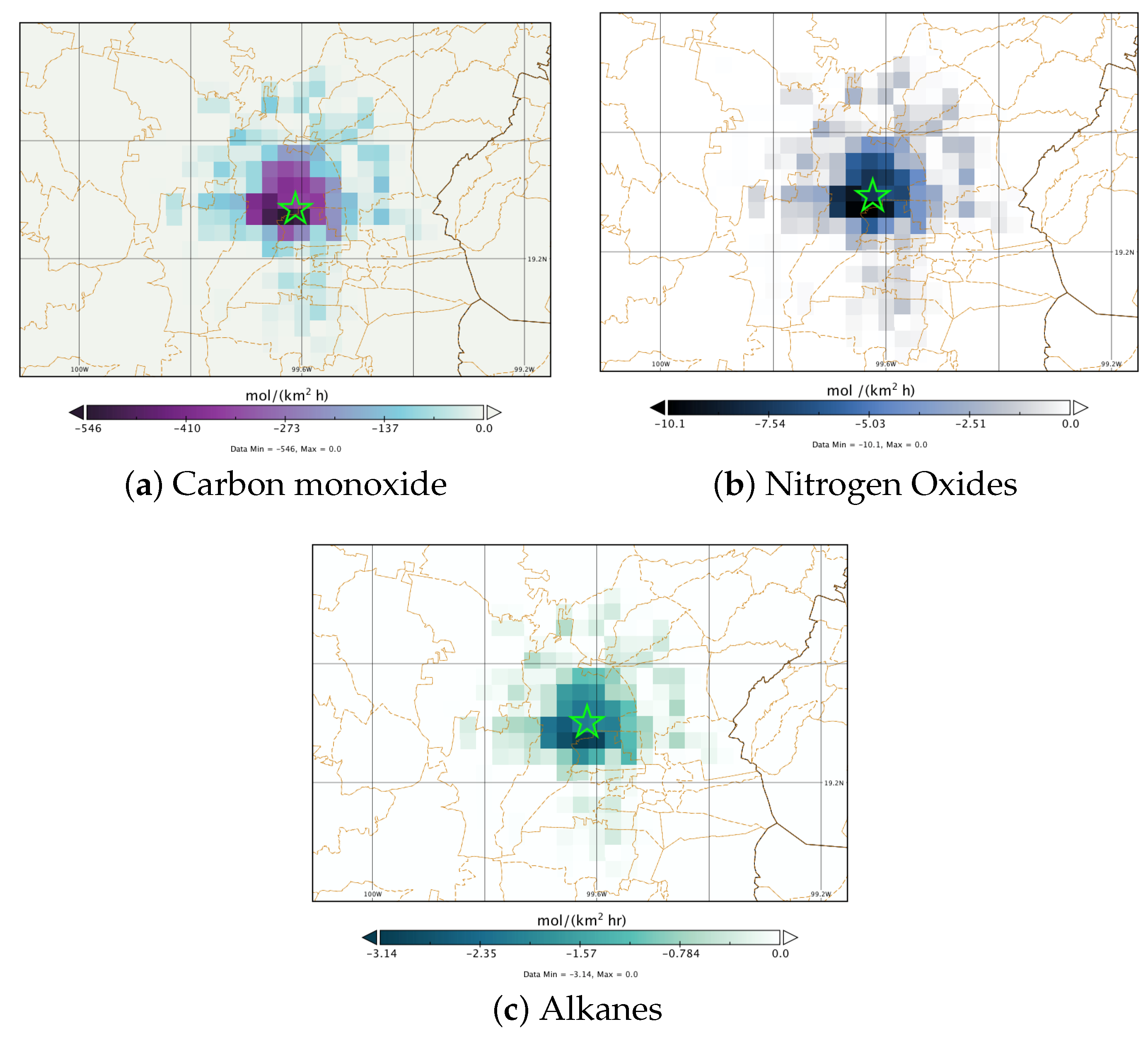
2.3.1. No-Driving Day Emission Scenario

The mobile emissions inventory for the Toluca Valley Metropolitan Area (TVMA) was first constructed for the base year 2019. We selected this year to avoid the massive reductions observed during the COVID-19 pandemics. The baseline inventory included particulate matter less than 10 and 2.5 micrometers (PM₁₀ and PM_2.5), sulfur dioxide (SO₂), carbon monoxide (CO), nitrogen oxides (NO_x), volatile organic compounds (VOCs), ammonia (NH₃), methane (CH₄), carbon dioxide (CO₂), nitrous oxide (N₂O), black carbon (BC), benzene, toluene, ethylbenzene, and xylene. All these emissions were calculated for both light and heavy-duty vehicles using the MOVES-Mexico model.

The No-Driving Day program (“Hoy No Circula”) reduction scenario was constructed based on the aforementioned 2019 base scenario of vehicular emissions and considering the two main tags assigned by the environmental authority. These tags are labeled Hologram 1 and Hologram 2, and correspond to vehicles with a model year older than 2006. Vehicles with Hologram 1 are considered to refrain from circulating one weekday per week and two Saturdays per month. Vehicles with Hologram 2 are considered to refrain from circulating one weekday per week and every Saturday of the month. This resulted in about 72,000 vehicles, representing roughly a 9% of the total fleet. These restrictions translate to:

• Hologram 1: Vehicles with hologram 1 would not circulate for 52 weekdays and 24 Saturdays, totaling 76 days per year.
• Hologram 2: Vehicles with hologram 2 would not circulate for 52 weekdays and 52 Saturdays, totaling 104 days per year.

The restricted days were applied to the corresponding vehicle fleet for both Hologram tags, resulting in a reduction in the circulating number of vehicles, a reduction in kilometers traveled, and an increase in their speed. This information was introduced into the MOVES Mexico model to estimate emissions for the No-Driving Day (NDD) scenario. The emission reduction was calculated as the difference between the base scenario and the NDD scenario.

To represent the possible application of the NDD to the TVMA, the main atmospheric species were reduced just for the mobile source sector.The estimated emissions reductions are presented in

Table 2. Emissions reductions due to application of the NDD scenario.

Compound		$\mathrm{\Delta }$ NDD (%)
Volatile Organic Compounds	VOC	21
Carbon monoxide	CO	19
Nitrogen oxides	NOx	15
Nitrogen dioxide	NO2	15
Ammonia	NH3	19
Sulfur dioxide	SO2	18
10 µm particles	PM10	21
2.5 µm particles	PM2.5	20
Carbon dioxide	CO2	17
Methane	CH4	16
Black carbon	BC	14

. These percentages are based on considerations of the vehicle fleet that considers light and heavy-duty vehicles that use either gasoline or diesel.

2.3.2. Model-Ready Emissions

The model-ready emissions files were generated with the DiETE emissions preprocessing system García-Reynoso et al. [29]. This required the use of the 2016 National Emissions Inventory (INEM), which was carefully scaled for the target year of 2019 following the method proposed by Rodríguez-Zas and Garcia [30].

The following figures depict the regional emissions reduction which was calculated as the difference between the scenario with the implementation of reductions due to the NDD program and the base case emissions scenario (baseline). Negative values indicate that emissions in the baseline case are higher than in the reduction scenario. The daily average emissions were speciated for the RADM2 chemical mechanism. Figure 3 illustrates the reduction only for the period from 6–8 May 2019; the other periods and pollutants presented a similar pattern.

The spatial difference fields show that the greatest reduction occurs towards the southwest center of the Toluca Valley Metropolitan Area (TVMA) for carbon monoxide, nitrogen oxides, and higher alkanes (HC8). Additionally, the emission reduction extends into parts of the peri-urban area. In this study, higher alkanes are considered representative of the feasible reduction in volatile organic compounds (VOCs).

2.4. External Transport

To investigate possible external transport into the TVMA, the HYSPLIT Lagrangian trajectory model [31,32] was run for the second simulation period (P2; 6–8 May 2019). Backward trajectories were obtained for 24 h, considering a height of 100 m above ground level. This height was chosen as it represents transport between the surface and the bottom of the boundary layer [33]. As an additional test, a height of 500 m was selected, but the results were very similar (not shown).

3. Results

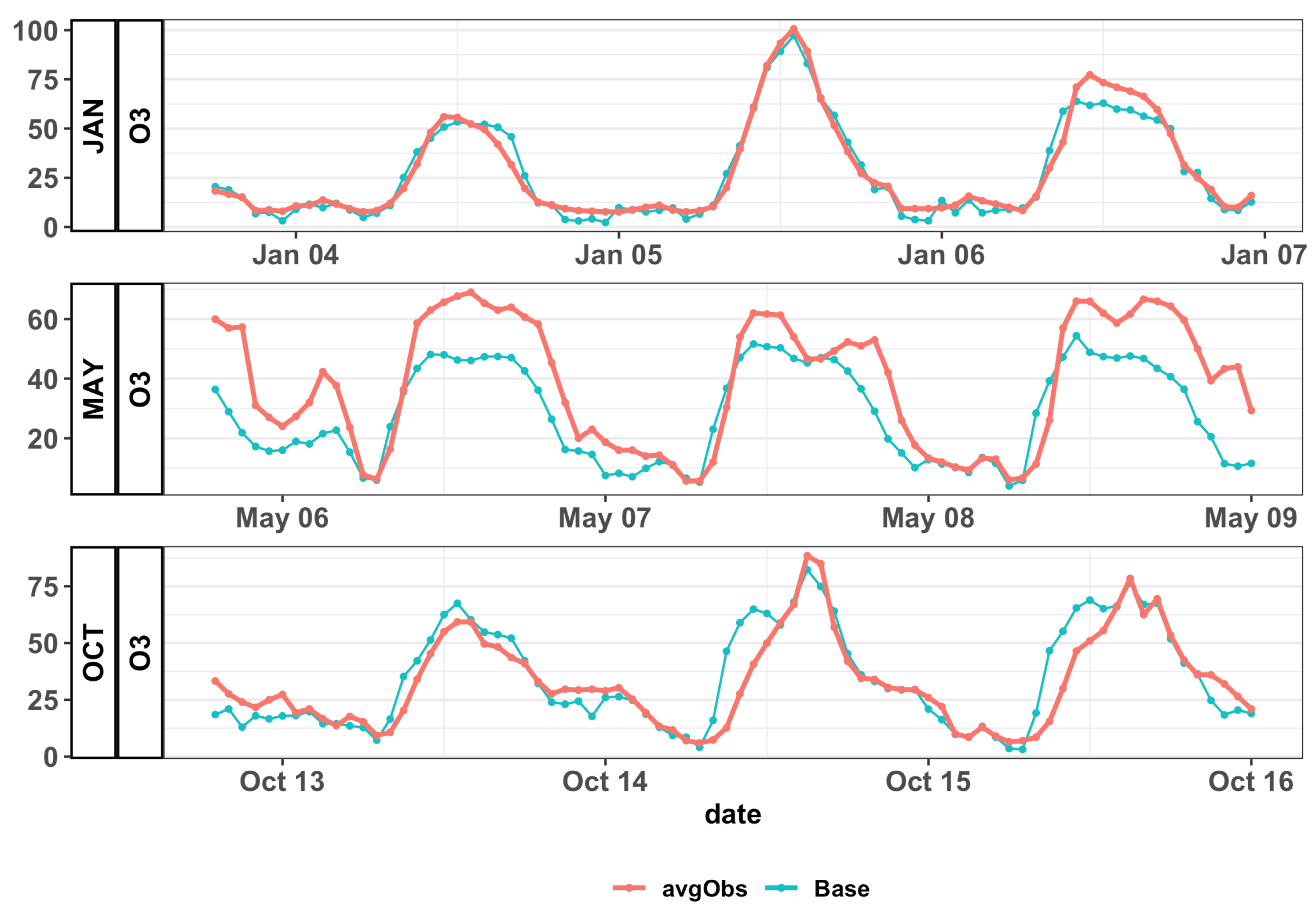
3.1. Model Evaluation

The model performance at the surface was evaluated against observations from the local monitoring network of the Toluca Valley Metropolitan Area (TVMA), following the methodologies outlined by García-Reynoso and Mora-Ramírez [34]. The variables considered included 2-meter temperature, carbon monoxide, nitrogen dioxide, sulfur dioxide, and ozone. Figure 4 presents the average model performance for the TVMA based on the six monitoring stations. Figure S1 shows the average model performance for temperature and wind velocity. Figure S2 shows the average model performance for CO, NO₂ and SO₂.

Table 3. WRF-Chem model performance for the 3 modeling periods. P1 (January 2019), P2 (May 2019) and P3 (October 2019).

Variable	RMSE			r			IOA
	P-Jan	P-May	P-Oct	P-Jan	P-May	P-Oct	P-Jan	P-May	P-Oct
O3 (ppb)	8.60	18.40	10.79	0.94	0.76	0.87	0.88	0.66	0.79
T (∘C)	2.40	1.80	1.86	0.96	0.98	0.97	0.79	0.84	0.78
CO (ppm)	432.50	421.00	359.10	0.84	0.81	0.61	0.65	0.55	0.44
NO2 (ppb)	12.50	9.10	9.04	0.62	0.77	0.51	0.53	0.68	0.31
SO2 (ppb)	2.60	2.60	1.96	0.41	0.54	0.37	0.46	0.29	0.37

presents the statistics for the root mean square error (RMSE), correlation coefficient (r), and the index of agreement (IOA) [35] during the three selected periods for the base case scenario.

Regarding temperature, an underestimation was observed in the daily maximum and an overestimation in the daily minimum, especially during the January (P1) and May (P2) periods. Conversely, for October, the model tended to underestimate both minimum and maximum temperatures. The lowest error and the best correlation were observed for the May period. A correlation close to 1 indicates that the model captured the diurnal profile well for all three periods. For wind, the model tended to overestimate wind speed compared to the observations from monitoring stations (Figure S1).

Nitrogen dioxide (NO₂) presented mixed results, with high RMSE values, ranging from 9.04 to 12.50 ppb, and varying correlation coefficients. The correlation coefficient (r) is generally moderate, with the highest correlation observed in May (0.77). However, the IOA values show variability, with the highest agreement in May (0.68) and the lowest in October (0.31).

For carbon monoxide (CO), the model tended to overestimate the maximum values and underestimate the minimum values in all three simulation periods. The RMSE in January and May was influenced by the underestimation during the morning period. However, the diurnal profile was relatively well captured except for October. Similarly, for nitrogen dioxide (NO₂), the model tended to overestimate the maximum values and underestimate the minimum values in all three simulation periods, shown for daylight hours, including the ozone peak. Unlike CO, the model predicted the time of maximum for NO₂ earlier in the morning and showed greater variability in all three periods, exhibiting a larger difference between the model results and observations, particularly in October, as reflected in the correlation coefficient.

Regarding SO₂, the evaluation is more qualitative as the observations are reported as rounded integers, preventing a detailed comparison with the model. However, in terms of magnitude and concentration maxima, the model performed well. Nevertheless, systematic errors were observed in the observations for some stations during the January and May periods, which tended to bias the estimation of the minimum, especially during the morning period. It is likely that the observations are not corrected for the background values.

For ozone, the model presented good performance (Figure 4). In January (P1) and October (P3), it slightly underestimated the maximum and replicated the daily minimum, as well as the timing of the peak. It also accurately represented the variability in both of these periods. However, in May (P2), the model considerably underestimated the maxima, although it slightly reproduced the hours when the peaks occurred. With respect to the January period (P1), the RMSE is more than double, and the correlation decreased significantly because the model did not fully capture the variability in the observations.

For the May period, a significant underestimation is observed during the daytime between 10 a.m. and 3 p.m. Additionally, the dynamics of the diurnal profile differ from those of the other periods. At the beginning of this period, a nighttime peak on 6 May is observed, followed by a second daytime peak on 7 May, and two additional daytime peaks on the last day of the period. These peaks indicate the presence of ozone produced outside the Toluca Valley Metropolitan Area (TVMA), which is transported from other regions and registered during the afternoon.

3.2. External Transport

Figure 5 shows a cluster of fires occurring in the central region of Mexico on 8 May 2019, as detected by the Terra product from the MODIS satellite. Additionally, it depicts the lines of the backward trajectories. Each backward trajectory spans 24 hours, with computations performed at three-hour intervals. The findings indicate that, during this modeling period, there was a notable transport phenomenon originating in the eastern side of Michoacan and in the western side of the State of Mexico. Consequently, the fires registered during this period likely had a significant contribution in ozone concentrations. Moreover, these transported air masses carry over photochemically aged material that not only influence local ozone formation, but also impacts the production of fine particles. As a result, the suboptimal model performance in May (P2) could be attributed to the regional transport of fire emissions, which were not considered in the configuration of the baseline case.

3.3. No-Driving Day

In this section, the results of the reduction scenario representing the implementation of the No-Driving Day (NDD) program are presented. Figure 6 illustrates the regional impact of the mobile source reduction measure through the NDD implementation in the Toluca Valley Metropolitan Area (TVMA) for specific days in each of the three simulation periods during daylight hours. For the January period (P1; Figure 6a), it is suggested that areas showing changes in ozone concentrations are close to the urban area, with decreases ranging from 4% to 7%.

For the May period (P2; Figure 6b), ozone levels tended to decrease downwind of the region where the reduction in vehicular emissions was applied. The estimated concentrations reductions ranged from 3.5% to 7.5% and included the daily peaks from 10 am to 3 pm. In contrast, in the area where emissions reductions (TVMA) are enforced, a marginal decreases in surface ozone concentrations was observed. Nevertheless, some areas presented small increases of up to 1% (white-colored area).

During the October period (P3; Figure 6c), surface ozone concentration over the TVMA presented more significant decreases than in the other two periods, with values between 2.5% and 9%. Additionally, unlike the other two periods, a more extended regional decrease is suggested for this period, reaching as far as Mexico City. However, ozone concentration increased southwest of the TVMA and southeast of Mexico City.

4. Discussion

The regional changes in ozone concentration after the introduction of a potential mitigation measure specific to the mobile sector in the Toluca Valley Metropolitan Area (TVMA) were estimated with a chemical transport model. Using an emissions inventory updated to 2019, the No Driving Day (NDD) mitigation measure was evaluated in three different periods representing three different meteorological conditions of the cold–dry (January and October) and hot–dry (May) seasons.

The application of the NDD mitigation measure in the TVMA could induce a reduction in ozone concentration between 3% and 8%, depending on meteorological conditions and the season of the year (cold–dry, hot–dry, and fire season). Due to the transport of primary pollutants, ozone production might be favored in downwind regions of the main emitting urban area so that a change in emissions results in changes in ozone concentrations in different areas from the emission source. In period 2 (P2; May), a downwind ozone production was estimated about 15 km from the TVMA. Thus, although the suggested reduction by the model is minimal within the Toluca Valley, it could have a downwind regional effect.

Another possible explanation of the small local impact of the NDD program in the Toluca urban area could be due to the small number of vehicles that were considered in the analysis. According to official data, a great amount of private cars are labeled with Hologram 0 and 00, which are exempted of the NDD restrictions. However, about 37% of the total private cars have a model year between 2000 and 2009, that is about 10 and 20 years old. Around 33% is classified within the model year of 2010–2019, that is of up to 10 years old. Thus, some relatively old vehicles, even around 18 years old, would be exempted from the restrictions.

In addition, it is assumed that, with the implementation of a NDD program, the travel speed could increase because it might reduce traffic congestion [10,36]. In Langang, China, traffic restrictions increased around 13% of the travel velocity in evening peak hours [36]. However, in this study, a conservative reduction of 5 km/h was input in the MOVES-Mexico model, with the assumption of a second car purchase and drivers that omit the restrictions.

Among the three selected simulation periods, the model performed well in those representing the cold–dry season and showed a considerable decrease in performance during the hot–dry season. A simple backward trajectory analysis suggested that transport of biomass burning emissions from southern regions in Michoacan and the State of Mexico could explain the additional variability and the late evening concentration peaks that are not measured in the other two periods. This indicates that, in some areas, ozone levels predominantly originate from other regions and possibly surpass locally generated levels. Spatial reductions in May (P2; Figure 6b) could be even smaller when fire emissions are included into the model.

The implication of this result is that biomass burning emissions could mask the possible benefits of implementing the NDD Program in Toluca. A recent study showed that, during the COVID-19 lockdown, fire emissions masked the effects of the strongest reductions in the Megalopolis of Mexico, including the TVMA [37]. For this reason, a policy oriented to biomass burning emissions at the regional level could be of aid in improving the regional air quality. For instance, alternative agricultural land management techniques that minimize emissions from burning, like chopping instead of burning might be considered in agricultural areas [38].

Some limitations in this study include the absence of biomass burning emissions in the simulations. In addition, the NDD emissions reduction scenario only included private cars.

Even though the length of the simulation periods might be short, they represent days with high ozone episodes and in different seasons. The first period (P1) includes a weekend. Future work will include the effect of biomass burning emissions in the regional chemical regimes and increasing the number of simulation periods. Despite their representing a small amount (∼ 15%) of the total vehicle fleet, there are still vehicles with model year of 1989 and older, which includes pickups and heavy trucks. A more detailed analysis will include the reduction of notoriously heavy-polluting vehicles.

5. Conclusions

This study estimated the regional impact of a mitigation measure specific of the mobile sector in the Toluca Valley Metropolitan Area (TVMA) in the cold–dry and hot–dry seasons. Although the possible reduction in ozone surface concentration might be small within the Toluca Valley after implementing the No-Driving Day emissions reduction program, there could be a reduction in downwind regions outside the Valley, which could possibly benefit Mexico City and the Megalopolis. The model effectively discerned the influence of these factors on ozone levels, demonstrating its utility in assessing the implementation of mitigation strategies and understanding the regional dynamics of air quality. The model presented a reasonable performance in reproducing CO, NO₂, SO₂ and ozone in three different simulation periods.

The identification of biomass burning as a significant contributor to ozone concentration during specific periods emphasizes the importance of considering external emissions sources in air quality management strategies. Additionally, the regional implications of emissions reductions, as seen in downwind effects, underscore the interconnected nature of air quality dynamics in neighboring areas.

The study not only provides insights into current air quality conditions in the TVMA, but also suggests potential measures to mitigate pollution, such as alternative agricultural land management practices. The consideration of these factors and the model capabilities contribute valuable information for decision-makers in developing effective air quality management policies tailored to the specific travel dynamics of the region.

This study also suggests that the continuous increase in mobility and the potential impact on air quality as a result of the increasing transportation needs in the suburban region around Toluca is essential to be considered in regional planning and air quality management of nearby air basins in a Megalopolis context.

References

1. Garcia, A. Diagnóstico Sobre la Calidad del Aire en Cuencas Atmosféricas de México; Final Report; Instituto Nacional de Ecología y Cambio Climático: Ciudad de México, México, 2016; Available online: https://www.gob.mx/cms/uploads/attachment/file/269889/Informe_Final_DCACAM.pdf (accessed on 3 February 2024).
2. Mario-Molina, C. Políticas Públicas para el Mejoramiento de la Calidad del Aire. Caso de Estudio: Zona Metropolitana del Valle de México; Final Report 1; Centro Mario Molina: Ciudad de México, México, 2014; Available online: https://centromariomolina.org/wp-content/uploads/2014/06/RE_HNC_ZMVM2014.pdf (accessed on 3 February 2024).
3. Ruiz-Suárez, G.; Calderón-Ezquerro, M.; Delgado-Campos, J.; Garcia-Martinez, R.; Garcia, A.; Grutter, M.; Molina, L.; Peralta-Rosales, O.; Torres-Jarcón, R.; Zavala-Hidalgo, J. Estudios de Calidad del Aire y su Impacto en la Región Centro de México; Final Report 2; Instituto Nacional de Ecología y Cambio Climático: Ciudad de México, México, 2015; Available online: https://www.gob.mx/cms/uploads/attachment/file/251716/Informe_Final_-_ECAICM_Tomo_2.pdf (accessed on 3 February 2024).
4. SEMARNAT. Inventario Nacional de Emisiones 2016; Technical Report; Secretaria del Medio Ambiente y Recursos Naturales: Ciudad de México, México, 2018; Available online: https://www.gob.mx/semarnat/documentos/documentos-del-inventario-nacional-de-emisiones (accessed on 27 February 2024).
5. WHO. WHO Global Air Quality Guidelines: Particulate Matter (PM2.5 and PM10), Ozone, Nitrogen Dioxide, Sulfur Dioxide and Carbon Monoxide; World Health Organization: Geneva, Switzerland, 2021; Available online: https://apps.who.int/iris/handle/10665/345329 (accessed on 3 February 2024).
6. CGCSA. Informe Nacional de la Calidad del Aire 2019; Technical Report; Instituto Nacional de Ecología y Cambio Climático: Ciudad de México, México, 2020; Available online: https://sinaica.inecc.gob.mx/archivo/informes/Informe2019.pdf (accessed on 3 February 2024).
7. Senado de Mexico. Dictamen; Gaceta LIX/3PPO-119-147/6290; Senado de la República: Ciudad de México, México, 2024; Available online: https://www.senado.gob.mx/65/gaceta_del_senado/documento/62905 (accessed on 27 February 2024).
8. Onursal, B.; Gautam, S. Vehicular Air Pollution: Experiences from Seven Latin American Urban Centers; World Bank: Washington, DC, USA, 1997; Available online: https://www.scopus.com/inward/record.uri?eid=2-s2.0-11344288688&partnerID=40&md5=2a4657954a34fc7197ac5832e241cab3 (accessed on 29 February 2024).
9. Davis, L.W. The Effect of Driving Restrictions on Air Quality in Mexico City. J. Political Econ. 2008, 116, 38–81. [Google Scholar] [CrossRef]
10. Sun, C.; Zheng, S.; Wang, R. Restricting driving for better traffic and clearer skies: Did it work in Beijing? Transp. Policy 2014, 32, 34–41. [Google Scholar] [CrossRef]
11. Davis, L.W. Saturday Driving Restrictions Fail to Improve Air Quality in Mexico City. Sci. Rep. 2017, 7, 41652. [Google Scholar] [CrossRef]
12. Tejeda-LeBlanc, D. Estudio Para el Análisis de Calidad del Aire en la Zona Metropolitana del Valle de Toluca para Determinar la Viabilidad de la Implementación del Acuerdo “Hoy No Circula”; LT Consulting: Ciudad de México, México, 2023; Available online: https://www.gob.mx/cms/uploads/attachment/file/892827/27_Informe_analisis_de_la_calidad_del_aire_ZMVT_prog_HNC.pdf (accessed on 27 February 2024).
13. Díaz-Ramírez, P.; García-Sosa, I.; Iturbe-García, L.; Granados-Correa, F.; Sánchez-Meza, C. Contaminación Atmosférica en el Valle de Toluca. Rev. Int. Contam. Ambient. 1999, 15, 13–17. Available online: https://www.revistascca.unam.mx/rica/index.php/rica/article/view/32632 (accessed on 27 February 2024).
14. Romero, G.E.; Sandoval, P.A.; Morelos, M.J.; Reyes, G.L. Chemical-morphological analysis and evaluation of the distribution of particulate matter in the Toluca Valley; Analisis quimico-mofologico y evaluacion de la distribucion de materia particulada en el Valle de Toluca. In Proceedings of the Memorias XVII Congreso Técnico Científico, Ciudad de México, México, 4–5 December 2007; Instituto Nacional de Investigaciones Nucleares: Ciudad de México, México, 2007; p. 5. Available online: https://www.osti.gov/etdeweb/servlets/purl/20995843 (accessed on 3 February 2024).
15. Ballesteros-Villegas, M.; Rotter-Zimbrón, C. Análisis de la Contaminación del Aire en los Municipios de Toluca, Metepec, San Mateo Atenco y Zinacantepec a Traves de la Metodologia de Simulacion Bajo el Metodo de Montecarlo, 2000–2020. Ph.D. Thesis, Universidad Autónoma del Estado de México, Toluca, México, 2014. Available online: http://hdl.handle.net/20.500.11799/63991 (accessed on 3 February 2024).
16. Ortinez, A.; Iniestra, R.; Basaldud, R.; Tzintzin, G.; Padilla, Z.; Fajardo, A.; Lopez, R.; Neda, R.C.; Aguirre, E.; Rodriguez, R. Evaluación de la Calidad del Aire en la Zona Metropolitana del Valle de Toluca Durante la Contingencia por COVID-19; Instituto Nacional de Ecología y Cambio Climático: Ciudad de México, México, 2020; Available online: https://www.gob.mx/cms/uploads/attachment/file/571385/Reporte_Toluca_COVID__Final.pdf (accessed on 3 February 2024).
17. Garcia, A.; Jazcilevich, A.; Ruiz-Suárez, L.; Torres-Jardón, R.; Suárez-Lastra, M.; Resendiz-Juárez, N. Ozone weekend effect analysis in Mexico City. Atmosfera 2009, 22, 281–297. Available online: https://www.revistascca.unam.mx/atm/index.php/atm/article/view/8627 (accessed on 3 February 2024).
18. Grell, G.A.; Peckham, S.E.; Schmitz, R.; McKeen, S.A.; Frost, G.; Skamarock, W.C.; Eder, B. Fully coupled “online” chemistry within the WRF model. Atmos. Environ. 2005, 39, 6957–6975. [Google Scholar] [CrossRef]
19. INECC. Sistema de Calculo de Indicadores de la Calidad del Aire. SEMARNAT. 2012. Available online: http://scica.inecc.gob.mx (accessed on 27 February 2024).
20. Chen, F.; Dudhia, J. Coupling an Advanced Land Surface–Hydrology Model with the Penn State–NCAR MM5 Modeling System. Part I: Model Implementation and Sensitivity. Mon. Weather Rev. 2001, 129, 569–585. [Google Scholar] [CrossRef]
21. Iacono, M.J.; Delamere, J.S.; Mlawer, E.J.; Shephard, M.W.; Clough, S.A.; Collins, W.D. Radiative forcing by long-lived greenhouse gases: Calculations with the AER radiative transfer models. J. Geophys. Res. Atmos. 2008, 113, D13. [Google Scholar] [CrossRef]
22. Hong, S.Y.; Noh, Y.; Dudhia, J. A New Vertical Diffusion Package with an Explicit Treatment of Entrainment Processes. Mon. Weather Rev. 2006, 134, 2318–2341. [Google Scholar] [CrossRef]
23. Hong, S.; Lim, J.O.J. The WRF Single-Moment 6-Class Microphysics Scheme (WSM6). Asia-Pac. J. Atmos. Sci. 2006, 42, 129–151. [Google Scholar]
24. Martilli, A.; Clappier, A.; Rotach, M.W. An urban surface exchange parameterisation for mesoscale models. Bound. Layer Meteor. 2002, 104, 261–304. [Google Scholar] [CrossRef]
25. Freitas, S.R.; Grell, G.A.; Li, H. The Grell–Freitas (GF) convection parameterization: Recent developments, extensions, and applications. Geosci. Model Dev. 2021, 14, 5393–5411. [Google Scholar] [CrossRef]
26. Stockwell, W.R.; Middleton, P.; Chang, J.S.; Tang, X. The second generation regional acid deposition model chemical mechanism for regional air quality modeling. J. Geophys. Res. Atmos. 1990, 95, 16343–16367. [Google Scholar] [CrossRef]
27. Vallamsundar, S.; Lin, J. Overview of US EPA new generation emission model: MOVES. Int. J. Transp. Urban Dev. 2011, 1, 39. [Google Scholar]
28. EPA Motor Vehicle Emission Simulator (MOVES). Environmental Protection Agency. 2024. Available online: https://www.epa.gov/moves/latest-version-motor-vehicle-emission-simulator-moves (accessed on 3 February 2024).
29. Garcia, A.; Mar-Morales, B.; Ruiz-Suarez, G. Spatial, temporal and speciation model of the Mexico national emissions inventory (base year 2008) for its use in air quality modeling (DiETE). Rev. Int. Contam. Ambient. 2018, 34, 635–649. [Google Scholar] [CrossRef]
30. Rodríguez Zas, J.A.; Garcia-Reynoso, J.A. Updating of the 2013 national emissions inventory for air quality modeling in central Mexico. Rev. Int. Contam. Ambient. 2021, 37, 463–487. [Google Scholar] [CrossRef]
31. Stein, A.F.; Draxler, R.R.; Rolph, G.D.; Stunder, B.J.B.; Cohen, M.D.; Ngan, F. NOAA’s HYSPLIT Atmospheric Transport and Dispersion Modeling System. Bull. Am. Meteorol. Soc. 2015, 96, 2059–2077. [Google Scholar] [CrossRef]
32. Rolph, G.; Stein, A.; Stunder, B. Real-time Environmental Applications and Display sYstem: READY. Environ. Model. Softw. 2017, 95, 210–228. [Google Scholar] [CrossRef]
33. Osibanjo, O.; Rappenglück, B.; Ahmad, M.; Jaimes-Palomera, M.; Rivera-Hernández, O.; Prieto-González, R.; Retama, A. Intercomparison of planetary boundary-layer height in Mexico City as retrieved by microwave radiometer, micro-pulse lidar and radiosondes. Atmos. Res. 2022, 271, 106088. [Google Scholar] [CrossRef]
34. Garcia, A.; Mora-Ramírez, M. Implementation of the Unified Post Processor (UPP) and the Model Evaluation Tools (MET) for WRF-chem evaluation performance. Atmosfera 2017, 30, 259–273. [Google Scholar] [CrossRef]
35. Willmott, C.J.; Robeson, S.M.; Matsuura, K. A refined index of model performance. Int. J. Climatol. 2012, 32, 2088–2094. [Google Scholar] [CrossRef]
36. Liu, Z.; Li, R.; Wang, X.; Shang, P. Effects of vehicle restriction policies: Analysis using license plate recognition data in Langfang, China. Transp. Res. Part Policy Pract. 2018, 118, 89–103. [Google Scholar] [CrossRef]
37. Almanza, V.; Ruiz-Suárez, L.G.; Torres-Jardón, R.; García-Reynoso, A.; Hernández-Paniagua, I.Y. Influence of biomass burning on ozone levels in the Megalopolis of Central Mexico during the COVID-19 lockdown. J. Environ. Sci. 2024, 143, 99–115. [Google Scholar] [CrossRef]
38. Pérez-Martínez, Z. De la Roza, Tumba y Quema a la Roza. Tumba y Pica. Technical Report. CIMMYT. 2022. Available online: https://www.cimmyt.org/es/noticias/de-la-roza-tumba-y-quema-a-la-roza-tumba-y-pica (accessed on 3 February 2024).
Figure 1. Simulation domain covered area. Toluca, State of Mexico capital located westward of Mexico City.
Atmosphere 15 00437 g001
Figure 2. Toluca air quality network.
Atmosphere 15 00437 g002
Figure 3. Differences in emissions between the control scenario and the base case in emissions for the May period in the TVMA (green star): (a) carbon monoxide emissions, (b) nitrogen monoxide emissions and (c) alkane emissions. The solid black lines denote the state political division and the dotted orange lines denote the municipalities.
Atmosphere 15 00437 g003
Figure 4. Average observed (red) and modeled (blue) ozone time series for the three modeling periods for the base case scenario. Units are in ppb.
Atmosphere 15 00437 g004
Figure 5. Fires and backward trajectories during 8 May 2019 obtained with the HYSPLIT model for the TVMA (White star).
Atmosphere 15 00437 g005
Figure 6. Estimated regional ozone reduction in the TVMA (red star) (%) for January (a), May (b) and October (c).
Atmosphere 15 00437 g006