Article

Traffic Flow Prediction Research Based on an Interactive Dynamic Spatial–Temporal Graph Convolutional Probabilistic Sparse Attention Mechanism (IDG-PSAtt)

1
State Environmental Protection Key Laboratory of Vehicle Emission Control and Simulation, Chinese Research Academy of Environmental Sciences, Beijing 100012, China
2
Institute of Advanced Technology, University of Science and Technology of China, Hefei 230000, China
3
Vehicle Emission Control Center, Chinese Research Academy of Environmental Sciences, Beijing 100012, China
*
Author to whom correspondence should be addressed.
Atmosphere 2024, 15(4), 413; https://doi.org/10.3390/atmos15040413
Submission received: 18 February 2024 / Revised: 14 March 2024 / Accepted: 21 March 2024 / Published: 26 March 2024
(This article belongs to the Special Issue Recent Advances in Mobile Source Emissions (2nd Edition))

Abstract

:
Accurate traffic flow prediction is highly important for relieving road congestion. Due to the intricate spatial–temporal dependence of traffic flows, especially the hidden dynamic correlations among road nodes, and the dynamic spatial–temporal characteristics of traffic flows, a traffic flow prediction model based on an interactive dynamic spatial–temporal graph convolutional probabilistic sparse attention mechanism (IDG-PSAtt) is proposed. Specifically, the IDG-PSAtt model consists of an interactive dynamic graph convolutional network (IL-DGCN) with a spatial–temporal convolution (ST-Conv) block and a probabilistic sparse self-attention (ProbSSAtt) mechanism. The IL-DGCN divides the time series of a traffic flow into intervals and synchronously and interactively shares the captured dynamic spatiotemporal features. The ST-Conv block is utilized to capture the complex dynamic spatial–temporal characteristics of the traffic flow, and the ProbSSAtt block is utilized for medium-to-long-term forecasting. In addition, a dynamic GCN is generated by fusing adaptive and learnable adjacency matrices to learn the hidden dynamic associations among road network nodes. Experimental results demonstrate that the IDG-PSAtt model outperforms the baseline methods in terms of prediction accuracy. Specifically, on METR-LA, the mean absolute error (MAE) and root mean square error (RMSE) induced by IDG-PSAtt for a 60 min forecasting scenario are reduced by 0.75 and 1.31, respectively, compared to those of the state-of-the-art models. This traffic flow prediction improvement will lead to more precise estimates of the emissions produced by mobile sources, resulting in more accurate air quality forecasts. Consequently, this research will greatly support local environmental management efforts.

1. Introduction

With the rapid development of urbanization and the growing complexity of road traffic networks, accurate traffic flow prediction has become an indispensable part of intelligent transportation systems (ITSs). Traffic flow prediction aims to predict future traffic flows based on a given historical traffic time series, and accurate traffic flow prediction is essential for transportation services, including route planning, congestion mitigation, and complex traffic network management. Traffic planning can improve the traffic environment, improve the quality of residents’ travel, and promote the sustainable development of cities. Through scientific planning, the rational use of land resources can be promoted, land use efficiency can be improved, and land waste can be reduced. Moreover, reasonable transportation system planning can reduce vehicle emissions and noise pollution, improve air quality, and improve residents’ travel comfort and safety.
Traffic flow prediction has always been a research hotspot in the field of ITSs, but due to the complex, non-Euclidean, and dynamic nature of road traffic networks, achieving accurate and efficient traffic flow prediction is still a significant challenge. Traffic flow data are time series data that have complex temporal dependencies and dynamic spatial correlations, as well as special periodicity, such as morning and evening peaks. Accurate traffic flow prediction requires a prediction model that can adequately capture long-term dependencies and dynamic spatial–temporal correlations.
First, in traffic flow prediction, the prediction error usually accumulates with the increase in time step. Even if the prediction in the first few time steps is relatively accurate, the error may gradually accumulate and expand with the passage of time. It can be challenging to estimate long-term traffic flows due to the complexity of temporal dependencies. For instance, when traffic conditions are predicted for the next 12 time steps by considering the traffic flows of the previous 12 time steps, the traffic flow predictions for the 9th–12th time steps are generally more difficult to obtain than those for the 1st–3rd time steps. Further complicating the task of precisely predicting traffic flows are the underlying dynamic spatial–temporal characteristics that result from the geographical heterogeneity, dynamic correlations, and uncertainty of transportation networks.
The complexity of a transportation network results in complex dynamic spatial–temporal interactions between traffic flows, as illustrated in Figure 1a, which demonstrates that spatial traffic conditions can influence each other and change over time. For instance, a traffic accident may impact the flows of traffic on surrounding roads, and the traffic flows in various directions on the same road might also be different. Figure 1b shows the hidden dynamic spatial characteristics of traffic flows, such as spatial heterogeneity, dynamic correlations, and uncertainty. The presence of distinct traffic patterns and spatial–temporal characteristics, such as residential and industrial zones, is what is meant by “spatial heterogeneity” [1]. Given historical traffic data and the topology of the associated road network, dynamic correlations refer to the associations between road network nodes over time. Uncertainty pertains to how a traffic flow is affected by accidents, holidays, severe weather, etc.
The ability to anticipate traffic flows using traditional machine learning techniques is severely constrained by their excessive reliance on feature engineering. Instead, deep learning-based approaches, which are frequently employed in traffic flow prediction applications, can efficiently and automatically extract data that describe traffic flow parameters. For instance, a spatial–temporal graph convolutional network (STGCN) [2] utilizes GCNs and gated linear units (GLUs) to capture the spatial–temporal correlations among traffic flows. To capture spatial–temporal correlations, Graph WaveNet [3] adapts both temporal convolutional networks (TCNs) and adaptive graph convolution. SLCNN [4] adapts dynamic graph convolution and a 1D convolutional neural network (CNN) [5] for exploring the spatial–temporal features between traffic flow nodes. STFGNN [6] utilizes multiple GCNs and 1D CNNs [7] to simultaneously extract spatial and temporal correlations. Several of the above studies employed serial or parallel structures to extract dynamic spatial–temporal features; however, these structures can weaken the captured spatial–temporal correlations and even amplify some irrelevant information, resulting in poor traffic flow prediction results. Therefore, the ASTGCN [8] employs a spatial attention mechanism and a temporal attention mechanism to further enhance the prediction performance of the model. The ASTGNN [9] adapts dynamic graph convolutions to extract spatial features and learns the temporal dependencies of traffic flows through an attention mechanism. Additionally, the AGCRN [10] embeds a spatial module into its temporal module, modifying an adaptive GCN and a gated recursive unit (GRU) [11] to enable the simultaneous capture of complex temporal dependencies and dynamic spatial features. MRA-BGCN [12] integrates an attention mechanism into its embedded structure to further extract dynamic spatial–temporal features. Although these methods have improved the ability to capture the dynamic spatial–temporal characteristics of traffic flows, the ability of spatial and temporal modules to interactively learn about and extract dynamic spatial–temporal features is poor, which affects the perception of the traffic flow prediction model with respect to the periodicity of the given time series and the trends of changes. This also results in the inability to adequately capture the dynamic spatial–temporal features of traffic flows [13].
Furthermore, many current studies represent the deep structure of a traffic flow by defining various adjacency matrices to capture hidden dynamic spatial features [14]. For instance, the MTGNN [15] employs GCNs, 1D CNNs, and adaptive adjacency matrices to learn hidden spatial features. The STSGCN [16] combines multiple adjacency matrices and employs an embedded structure for traffic flow prediction purposes. An adaptive adjacency matrix can explore the hidden relationships among road network nodes to improve the ability of the utilized model to learn about the spatial heterogeneity of traffic flows; however, with the cessation of the model training process, the adaptive adjacency matrix cannot learn the dynamic associations among graph nodes over time, which leads to the inability of the model to make full use of historical traffic flow information [17]. Therefore, the above methods still cannot fully and effectively capture the hidden spatial features of traffic flows.
To address the above research challenges, a traffic flow prediction model based on an interactive dynamic spatial–temporal graph convolution probabilistic sparse attention mechanism (IDG-PSAtt) is proposed; this model adequately extracts dynamic spatial–temporal features from traffic flow time series. A dynamic GCN (DGCN) that can fully utilize a priori knowledge to generate dynamic graphs for capturing the hidden spatial features of traffic flows is adapted. The DGCN is embedded into an interactive learning structure to form an interactive dynamic GCN (IL-DGCN), which analyses the periodicity of the traffic flows, divides the sequences into intervals, and then captures their deep dynamic spatial–temporal features through interactive learning among the divided subsequences. The IDG-PSAtt model combines multiple IL-DGCN modules through an interactive learning strategy to fully extract the dynamic spatial–temporal features of traffic flows. In addition, an adaptive adjacency matrix and a dynamic adjacency matrix are used to further explore the dynamic associations between nodes over time. Finally, IDG-PSAtt captures the complex temporal dependence at the same location and the dynamic spatial correlations among traffic flows at neighboring locations at the same time step via a spatial–temporal convolution (ST-Conv) block; it also employs a probabilistic sparse self-attention (ProbSSAtt) mechanism to incorporate dynamic spatial–temporal features and reduce the computational complexity of the model.
Traditional convolutional networks are only applicable to extracting the local features of Euclidean data, whereas traffic flows are non-Euclidean data. A GCN extends the traditional convolution process to graph-structured data and learns the neighbor information of nodes and edges to process non-Euclidean data and capture the dynamic spatial features of non-Euclidean data [18]. Currently, GCNs are mainly categorized into two types of methods, as follows: null domain and spectral domain methods. GCNs based on null domain methods perform convolution by aggregating node information from neighbors to capture the features of the nodes, but the node neighborhood selection process of this method is extremely difficult [19]. A combination of null domain-based GCNs and an attention mechanism was used to dynamically adjust the weights of neighboring nodes for determining the importance of these nodes in [20]. A GCN based on the spectral domain aggregates the neighbor information of each node through a spectral analysis conducted over the entire graph and the entire graph must be processed at once, which is computationally complex. Deng et al. [21] mapped the structure of a topological graph in the null domain to the spectral domain through the Fourier transform to perform a convolution operation and then used an inverse transformation back to the null domain to complete the computation. Yan et al. [22] adapted ChebNet [23] to decrease the computational complexity of the Laplacian and enhance the performance of traditional GCNs. Based on the graph convolution framework, Li et al. [2] utilized gated GCNS to capture the dynamic features of traffic flows; however, their model does not consider the dynamic spatial–temporal dependencies of traffic flows.
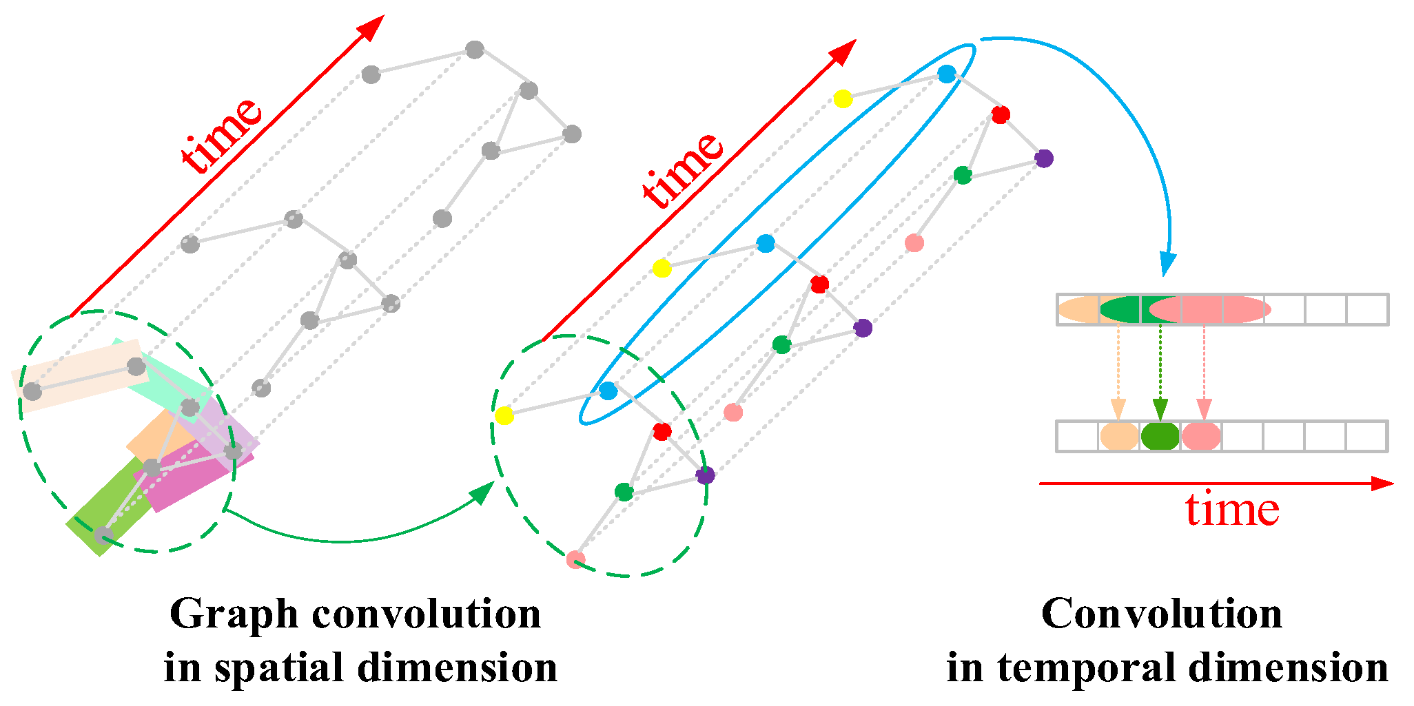
Two main STGCN approaches are available, as follows: artificial neural network (RNN)-based and CNN-based methods [24]. An RNN-based STGCN can learn the temporal dependencies of traffic flows, but the iterative RNN training process leads to problems such as error accumulation, a slow training speed, and the inability to handle long time series [25]. For example, the spatial–temporal features required for traffic flow prediction can be captured by using an RNN-based graph convolutional recurrent unit network that simultaneously filters inputs and hidden states, but this method is not able to effectively capture dynamic spatial–temporal correlations and has poor long-term prediction capabilities [26]. In contrast, CNN-based STGCNs can process data in parallel and consume less memory, significantly improving the training speed of these models; however, when the number of layers in an STGCN is too deep, data feature extraction difficulties are encountered. In addition, the incorporation of a long short-term memory (LSTM) network into a CNN-based STGCN can enable it to efficiently process complex time series. Therefore, Chen et al. [27] processed the dynamic spatial–temporal information of road networks and, thus, predicted future traffic flow through a CNN and LSTM. The common STGCN structure is shown in Figure 2. An STGCN consists of a graph convolution in the spatial dimension and a one-dimensional standard convolution in the temporal dimension, which capture the hidden spatial features of neighborhood locations and the complex temporal dependencies at different times, respectively.
In addition, with the rapid development of attention mechanisms, these mechanisms have been widely used in many fields, such as image processing, speech recognition, and natural language processing. They are especially utilized in the field of ITSs to assist in the long-term prediction of traffic flows [28]. For example, a spatial–temporal graph convolution prediction model can be constructed by means of a spatial–temporal graph convolution and a self-attention mechanism to capture the dynamic spatial–temporal features of traffic flows. Zheng et al. [29] proposed a GCN based on a self-attention mechanism; this GCN inherits the advantages of the self-attention mechanism and can capture the dynamic spatial–temporal dependencies of traffic flows. Zheng et al. [30] utilized an encoder–decoder structure composed of spatial–temporal attention modules to capture the spatial–temporal features of traffic flows. Guo et al. [9] presented an attention-based spatial–temporal GNN (ASTGNN), which captures complex temporal dependencies through trend-aware self-attention modules and utilizes a DGCN to extract dynamic spatial features. Although the above methods enhance the prediction performance achieved by the associated models by using self-attention mechanisms, most of these studies tended to ignore the stacked implicit relationships and hidden spatial–temporal correlations in the channel dimensions, weakening the ability of their models to capture dynamic spatial–temporal features.
Inspired by the above studies, by combining the spatial heterogeneity, dynamic correlations, and uncertainty of road traffic networks, as well as the non-Euclidean data [31] characteristics of traffic flows, a traffic flow prediction model called IDG-PSAtt is proposed. The combination of an interactive dynamic convolution structure with spatial–temporal convolution and a ProbSSAtt block fully captures the dynamic spatial–temporal features of the input traffic flow time series. The IL-DGCN adopts interactive learning to curate traffic flow data into segments at intervals and then synchronously extracts the spatial–temporal dependencies of the segmented sequences and shares the learned spatial–temporal features between the sequences. The ProbSSAtt block improves the computational efficiency of the model by adjusting its attention coefficients so that a small number of key points in the traffic flow provide the main attention for reducing the computational complexity. The interactive learning strategy and the ProbSSAtt block enable the IDG-PSAtt model to effectively perform long-term prediction. In addition, this paper constructs a dynamic GCN through an unusual dynamic graph generation approach to capture the hidden dynamic correlations among traffic flow nodes and thus capture the dynamic spatial correlations of the traffic network. Finally, the dynamic spatial–temporal characteristics extracted by adapting the multihead ProbSSAtt block are adaptively fused in this research by employing the gated fusion technique, which mitigates the propagation of errors and increases the resulting prediction accuracy.
The main contributions of this paper are summarized below.
  • A traffic flow prediction model based on IDG-PSAtt is proposed; this model embeds a DGCN into an interactive learning structure and inherits the advantages of spatial–temporal convolution, as well as a ProbSSAtt block to capture long-range dynamic spatia–temporal features.
  • A DGCN is constructed to capture spatial–temporal features; this network is generated via the fusion of an adaptive adjacency matrix and a learnable adjacency matrix, where the adaptive adjacency matrix captures the heterogeneity of the given traffic flow time series and the learnable adjacency matrix learns the dynamic correlations among the nodes of the road network.
  • An ST-Conv block is designed, and the ProbSSAtt block is introduced; these blocks learn the hidden spatial features among various nodes and the complex spatial–temporal dependencies to improve the computational efficiency of the model.
  • Several comparative experiments are conducted on two datasets and the results show that the IDG-PSAtt model achieves the best prediction performance in both cases when compared to the existing baseline methods.
  • The traffic flow prediction model proposed in this paper can guide the transportation planning process, thus improving the transportation environment, enhancing the quality of residents’ travel, and promoting the sustainable development of cities.

2. Methodology

2.1. Problem Definition

This paper represents a road traffic network as a graph G = V , E , A , where V = N is the set of nodes; E is the set of edges between the nodes, whose weights are represented by the distances between the nodes; and A N × N denotes the initial adjacency matrix generated by the graph G ; if v i , v j V and v i , v j E , A i j is 1; otherwise, A i j is 0. The traffic flow prediction task aims to predict a future traffic flow based on the given historical information. The adjacency matrix A obtained from the original traffic network is used as a priori knowledge to predict future traffic flows X G t + 1 , X G t + 2 , , X G t + T through the historical time series X G t T + 1 , X G t T + 2 , , X G t , where X G t N × C denotes the observation value of graph G at time t , C denotes the number of feature channels, T denotes the length of the given historical time series, and T denotes the length of the predicted future traffic series. The mapping relationships in the traffic flow prediction problem can be expressed as follows:
X G t T + 1 , X G t T + 2 , . . . , X G t f X G t + 1 , X G t + 2 , . . . , X G t + T
where f denotes a prediction function that is capable of predicting future traffic flows from a given historical time series.

2.2. Framework of IDG-PSAtt

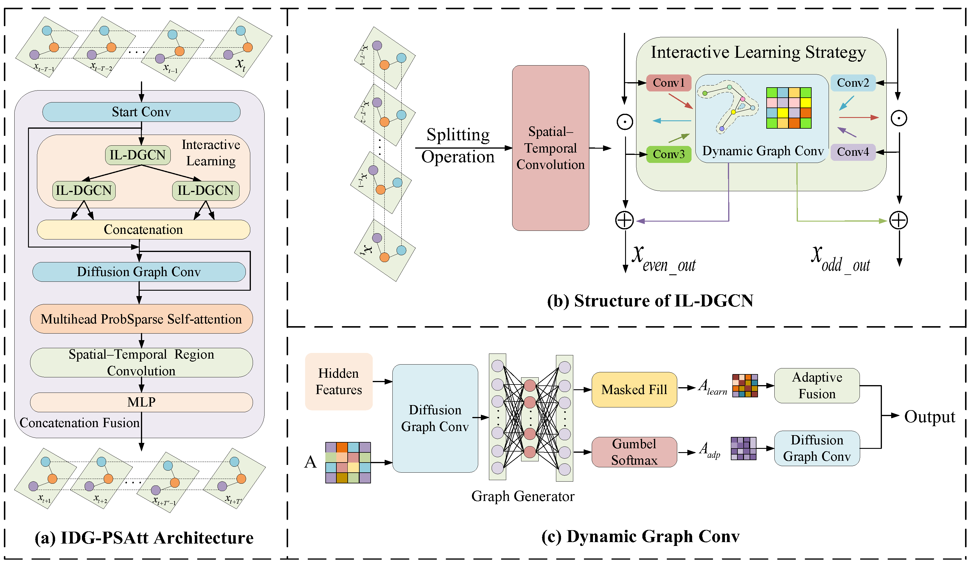
The IDG-PSAtt model is proposed for simultaneously capturing the dynamic spatial–temporal correlations of traffic flows. The overall framework of IDG-PSAtt is shown in Figure 3; this framework consists of an IL-DGCN, a tandem fusion module, an ST-Conv block, and a ProbSSAtt block. Among them, the IL-DGCN can extract the hidden dynamic spatial features and dynamic relationships between nodes over time.
First, this paper feeds the raw data into a Start Conv layer to obtain a high-dimensional spatial representation of the data for capturing deeper dependencies; then, the IL-DGCN processes the features extracted from the Start Conv layer with an interactive learning strategy implemented on top of the DGCN. The original input of the IL-DGCN is recursively generated by performing interleaved sampling in the data division phase to generate two subsequences of equal size (halved in length); then, the IL-DGCN interactively learns these two subsequences and shares the features learned by each of them. By embedding the DGCN into the interactive learning structure, the dynamic spatial features of traffic flows are interactively acquired, while capturing their temporal dependencies. After the IL-DGCN extracts spatial–temporal features, two subsequences are output. Through the tandem fusion module, both output subsequences are reorganized in time order and then fed to diffusion graph convolution and ST-Conv blocks to extract the global dynamic spatial–temporal features of the traffic flows. Finally, the captured dynamic spatial–temporal features are fed to the ProbSSAtt block and a multilayer perceptron (MLP) to output the predicted sequence.

2.2.1. Interactive Learning

In this paper, an interactive learning module is implemented with a CNN and a GCN, which can efficiently process non-Euclidean data, better learn the spatial–temporal dependencies of traffic flows, and more adequately capture complex temporal features and dynamic spatial features than can CNN- and TCN-based methods. Moreover, since traffic flows are periodic, trending, and similar, the interleaved sampled subsequences still retain most of the information of the original sequence; therefore, this paper employs the interleaved sampling method to process the original data for performing multiresolution analyses and expanding the sensory field. The interactive learning framework in this paper consists of three identical IL-DGCNs, the core of which is the IL-DGCN module. In the IL-DGCN, two subsequences interactively learn their respective dynamic spatial–temporal features, and each subsequence preprocesses the features via convolution to expand the receptive domain. Moreover, the two subsequences share parameter weights in the DGCN and capture dynamic spatial–temporal features from each other.
In this paper, X C × N × T denotes the input of the IL-DGCN, and X obtains two subsequences after performing interleaved sampling, as follows: an odd sequence X o d d R C × N × T 2 and an even sequence X e v e n C × N × T 2 . Moreover, C o n v 1 , C o n v 2 , C o n v 4 , and C o n v 4 in the IL-DGCN denote 1D convolution operations. The outputs of the first interactive learning process of the IL-DGCN are X o d d C × N × T 2 and X e v e n R C × N × T 2 . Through additional interactive learning, X o d d and X e v e n obtain the final output sequences X o d d _ o u t C × N × T 2 and X e v e n _ o u t C × N × T 2 .
The specific operations in the interactive dynamic graph convolution process are denoted as follows:
X e v e n , X o d d = S p l i t X
X o d d = σ D G C o n 1 X e v e n X o d d
X e v e n = σ D G C o n 2 X o d d X e v e n
X o d d _ o u t = X o d d + σ D G C o n 3 X e v e n
X e v e n _ o u t = X e v e n + σ D G C o n 4 X o d d
where denotes the Hadamard product and t a n h denotes the activation function.

2.2.2. Dynamic Graph Convolution

The DGCN in this paper mainly consists of a diffusion GCN and a graph generation module to better learn deep dynamic spatial features for enhancing the performance of the IDG-PSAtt approach in terms of capturing spatial heterogeneity. The DGCN feeds the hidden features H C × N × T and the predefined initial adjacency matrix A R N × N as inputs to the diffusion GCN, which is subsequently fed to the generator and MLP layers to generate discrete matrices A N × N containing spatial–temporal information. A is represented as follows:
A = σ M L P G H , A
where G C N denotes the diffusion convolution and graph generation operations and M L P denotes the multilayer perceptron.
Gumbel reparameterization is used in this paper because of the need to ensure that the sampling process is conductible during training:
A l e a r n = G u m b e l S o f t max A = σ log A log log g / τ
where g G u m b e l 0,1 denotes a random variable, τ is the softmax temperature and has a value of 0.5, and A l e a r n denotes the adjacency matrix generated by a graph generator that can simulate the dynamic dependencies between nodes.
Moreover, this paper constructs an adaptive adjacency matrix A a p t N × N , which is denoted as follows:
A a p t = σ R e l u E 1 E 2 T
where E 1 N × c and E 2 T R N × c denote the learnable parameters, and the initial value of A a p t is a predefined adjacency matrix A N × N , based on the original graph data.
In this paper, we extract the hidden dynamic spatial–temporal correlations among road traffic flows by fusing A l e a r n and A a p t with an adaptive fusion module and then feeding the resulting dynamic adjacency matrix A d y n N × N to a diffusion GCN. The specific operation of this fusion module is as follows:
A d y n = α A a p t + 1 α A l e a r n
where α denotes the learnable adaptive parameter
This paper utilizes diffusion graph convolution and fusion graph convolution and uniformly defines the diffusion graph convolution input as X i n C × N × T .
The diffusion graph convolution process is defined as follows:
G X i n , A a p t = k = 0 K A a p t k X i n W
where k is the diffusion step size, K is the maximum number of diffusion steps, and W is the parameter matrix.
The adjacency matrix of the fusion graph convolution input, denoted by the symbol A d y n in the fusion graph convolution module, is represented as follows:
G X i n , A d y n = k = 0 K A d y n k X i n W
The IDG-PSAtt model feeds the dynamic spatial–temporal characteristics extracted from the interactive learning structure to the diffusion graph convolution module by recombining them in the concatenation module in time order to capture and correct all the time series features.
Different from previous studies, this paper uses both the predefined initial adjacency matrix A N × N and the dynamic adjacency matrix A d y n R N × N obtained by the interactive learning structure in the diffusion graph convolution module. For the initial adjacency matrix A , this paper uses directed graphs as well as P f = A r o w s u m A and P b = A T r o w s u m A T to denote the forward and backward transfer matrices of A , respectively. In this case, the diffusion map convolution process in the concatenation fusion module is represented as follows:
G X i n , A , A d y n = k = 0 K A f k X i n W 1 + A b k X i n W 2 + A d y n k X i n W 3
The DGCN module is capable of extracting deep hidden spatial features by exploring the invisible dependencies between nodes in the traffic network and generating dynamic correlations between data based on the simulation of the input traffic flow time series. In addition, by embedding a DGCN into the interactive learning framework, it is possible to make full use of the dynamic spatial information captured by the DGCN to more effectively capture the complex temporal dependencies of traffic flows during the training process.

2.2.3. ST-Convolution Block

In a road traffic network, the data detected by each sensor exhibit a certain degree of periodicity. For example, during the morning and evening peak phases on weekdays, the traffic flow increases significantly and its speed is generally low. The hidden spatial features of traffic flows are related to the distances between different sensors and these spatial features are not affected by temporal dependence.
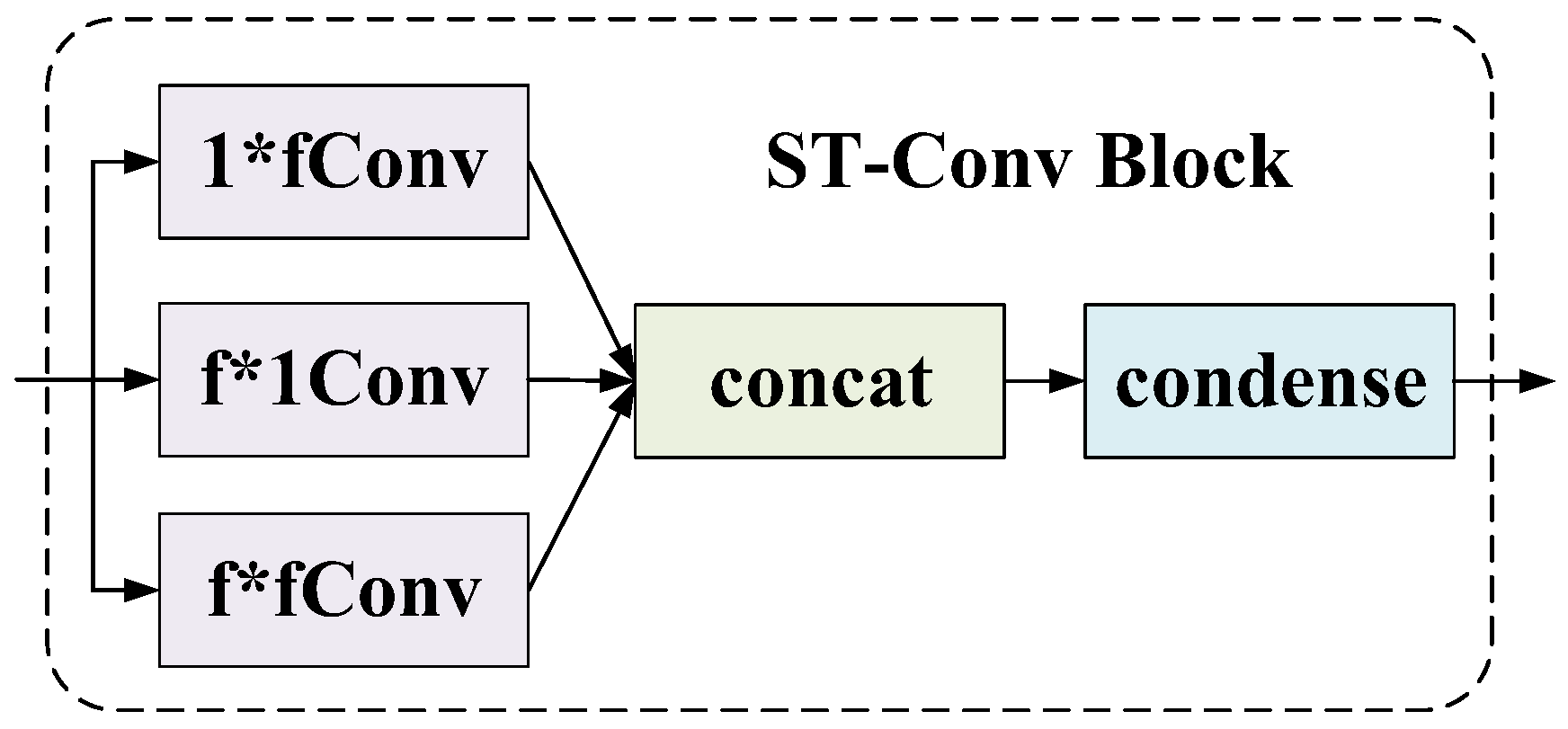
In this paper, a spatial–temporal convolution module consisting of three kernels is designed, as shown in Figure 4. The three kernels correspond to the temporal, spatial, and spatial–temporal perspectives for capturing the spatial–temporal features extracted from the diffusion graph convolution module and the influences of multiple node features on a single node feature in the topological graph structure of the traffic flow. The temporal kernel captures the dependencies of traffic flows at different times at the same location, and the spatial kernel captures the spatial correlations of traffic flows at neighboring locations during the same time step. The output of the prior spatial–temporal attention block serves as the input for each subsequent spatial–temporal convolutional block, i.e., X N l R C l × V N × T h . The output X N l + 1 can be calculated from Equations (14) and (15).
H = σ ϖ s t l + 1 X N l ; ϖ t l + 1 X N l ; ϖ s l + 1 X N l ;
X N l + 1 = σ ϖ o l + 1 H
where ϖ t l + 1 is the temporal kernel with a size of f × 1 , ϖ s l + 1 is the spatial kernel with a size of 1 × f , and ϖ s t l + 1 is the spatial–temporal kernel with a size of f × f . L e a k y R e L U denotes the L e a k y rectified linear unit function and denotes the convolution operation. Finally, the outputs of the three convolution kernels are concatenated and the 1 × 1 convolution ϖ o l + 1 is used to compress the features and limit the number of channels.

2.2.4. Subsubsection

A typical input of a self-attention mechanism possesses the form Q , K , V and the dot product operation is computed as follows:
A Q , K , V = σ Q K T d V
where Q R L Q × d , K R L K × d , V R L V × d , and d denote the input queries, keys, values, and dimensionality, respectively. The attention factor A q i , K , V for the i -th query is as follows:
A q i , K , V = j k q i , k j l k q i , k l v j = E p k j | q i v j
where q i , k i , and v i are the i th rows in Q , K , and V , respectively. p k j | q i = k q i , k j l k q i , k l and k q i , k l use the asymmetric index kernel exp q i k j T d .
The spatial complexity of the self-attention mechanism for computing the dot product p k j | q i is O L Q L K . However, in the computation of the ProbSSAtt block, the input lengths of the query and the key are usually equivalent, i.e., L Q = L K = L , resulting in a total temporal and spatial complexity of O L ln L . In addition, the ProbSSAtt block combines probabilistic sparsity and a self-attention mechanism by adjusting the attention coefficients on top of the self-attention mechanism so that for each query, only some of the keys are important to it, i.e., a few key dot products provide the main attention and the remaining dot products are neglected. This approach can indirectly combine complex time-dependent and dynamic spatial features to save computational resources without affecting the accuracy of the model.
STC-ProbSSAtt uses M q i , K to denote the sparsity of the i th query and K L scatter to measure the sparsity of the query as follows:
M q i , K = ln j = 1 L K e q i k j T d 1 L K j = 1 L K q i k j T d
where the arithmetic mean of all keys is the second term, and the first term is the logarithm and exponent of q i for all keys. It is possible to create the ProbSparse self-attention mechanism using this idea.
A Q , K , V = σ Q - K T d V
The constant sample factor c controls u = c ln L Q , and Q - designates the same sparse matrix as that in dimension q . Q - includes only the first u queries under the sparsity evaluated using M q , K . As a result, the queries of the ProbSparse self-attention mechanism have only O ln L Q complexity. To prevent major information losses, we adopt the multihead ProbSparse self-attention technique in this study. This mechanism may provide various sparse query–key pairs.

2.3. Data Description

The prediction performance achieved using the IDG-PSAtt model on the METR-LA and PEMS-BAY [32] public transportation datasets is validated in this study. The METR-LA dataset, rooted in the bustling urban sprawl of Los Angeles County, provides a rich vein of data reflecting the dynamic nature of traffic flows on its freeways. This dataset’s significance is amplified by its detailed capture of traffic speed statistics, offering a granular look at vehicular movement patterns over a four-month period through the lens of 207 strategically placed sensors. The PEMS-BAY dataset serves as a complementary yet distinct counterpart, focusing on the San Francisco Bay Area’s traffic arteries. With a broader temporal scope spanning six months, it encompasses traffic speed data collected by 325 sensors. The detection site, detection date, and data type are all recorded by METR-LA and PEMS-BAY. Table 1 displays specific information about the experimental datasets.
Since the METR-LA dataset is missing some data, the missing values are filled in by conducting linear interpolation during the experiment. Before the data are input into the prediction model, the data are min–max normalized to restrict the data to [0, 1].

2.4. Evaluation Metrics

In this paper, traffic flows for 12 consecutive time steps during the past hour are utilized to predict future traffic flows for 12 consecutive time steps during the next hour. In the experiment, the dataset is chronologically divided into training, test, and validation sets at a ratio of 7:2:1 for predicting traffic flow forecasts at 15 min, 30 min, and 60 min. Moreover, three standard metrics, the mean absolute error (MAE), root mean square error (RMSE), and mean absolute percentage error (MAPE), are used in this paper to evaluate the prediction performance of all the tested methods and are defined as follows:
M A E = 1 N i = 1 N y i y ^ i
R M S E = 1 N i = 1 N y i y ^ i 2
M A P E = 100 N i = 1 N | y i y ^ i y i |
where N is the number of observations and y i and y ^ i denote the actual and predicted traffic speeds, respectively. The smaller the predicted MAE, RMSE, and MAPE values are, the better the prediction performance of the IDG-PSAtt model.

2.5. Baselines

In this paper, we compare the IDG-PSAtt model with the following baseline models.
(1)
HA [33]: The average values of the historical and current traffic flows are used as the prediction values for the next step. In the baseline method, the average of the past 12 time slices in the same period as a week ago is utilized to forecast the current time slice.
(2)
VAR [34]: This method represents vector autoregression.
(3)
SVR [35]: This is an extension of support vector machine (SVM) classification for regression problems. According to the grid search method, the insensitivity loss coefficient ε is set to 0.1 and the penalty factor C is set to 1.0.
(4)
FNN [7]: This is a two-hidden-layer feedforward neural network using L2 regularization.
(5)
ARIMA [36]: This is a popular model used in time series prediction tasks. The orders of the autoregression, difference, and moving average operations are the three crucial parameters for the ARIMA model, (p, d, q) is set to (4, 1, 1).
(6)
FC-LSTM [37]: This is a classic RNN that learns time series and makes predictions via fully connected neural networks, a single hidden layer with 64 hidden units is utilized.
(7)
WaveNet [38]: This is a CNN for predicting sequence data, there are 8 stacked layers with a specific dilation rate of [1, 2, 1, 2, 1, 2, 1, 2, 1, 2], and the hidden dimension is set to 64.
(8)
Graph WaveNet [3]: This network is constructed with a GCN and a gated temporal convolution layer (gated TCN), there are 8 stacked layers with a specific dilation rate of [1, 2, 1, 2, 1, 2, 1, 2, 1, 2], and the hidden dimension is set to 64.
(9)
STGCN [2]: This network employs graph convolutional layers and convolutional sequence layers, there are 2 spatiotemporal cells and the hidden dimension is set to 64.
(10)
ASTGCN [8]: This model employs an attention mechanism to capture spatiotemporal dynamic correlations, there are 2 spatiotemporal cells and the hidden dimension is set to 64.
(11)
STSGCN [16]: This model individually captures localized spatial and temporal correlations, the number of STSG layers is set to 3 and the hidden dimension is set to 64.

3. Results and Discussion

This paper compares the performance of the IDG-PSAtt model with that of 11 common baseline models for 15, 30, and 60 min predictions. On two datasets, the IDG-PSAtt model achieves the best prediction results in terms of all the evaluated metrics.
The experimental results in Table 2 indicate that the statistical approaches (HA, VAR, and ARIMA) and the traditional machine learning approaches (SVR and FC-LSTM) perform poorly because these models only consider temporal dependencies and ignore the dynamic spatial characteristics of traffic flows. GCN-based models can handle non-Euclidean traffic data and capture the hidden relationships among road network nodes more effectively; thus, the STGCN and STSGCN models with spatial–temporal GCNs perform better. Although the STSGCN model is capable of concurrently capturing spatial and temporal data, it performs inadequately since it only emphasizes capturing temporal dependencies and uses a straightforward sliding window to capture temporal correlations. Additionally, since attention mechanisms capture the temporal dependencies of sequences, models based on attention mechanisms (e.g., the ASTGCN) also perform well. Graph WaveNet embeds a GCN into a TCN, which makes its performance better than that of the ASTGCN, but Graph WaveNet does not incorporate a self-attention mechanism to further capture the hidden spatial–temporal features.
The IDG-PSAtt model significantly improves upon the state-of-the-art models on the METR-LA and PEMS-Bay datasets for 15, 30, and 60 min predictions, because the IDG-PSAtt model adequately captures the dynamic spatial–temporal features of traffic flows through interactive learning structures, its DGCN, and its ST-Conv block; it also utilizes the ProbSSAtt block to produce effective long-range predictions. For instance, the IDG-PSAtt model outperforms the state-of-the-art methods in terms of the MAE, RMSE, and MAPE metrics by 29.4% and 32.2%, respectively, as well as by 9.4%/8.3% and 15.5%/16.1%, respectively, for 15 min and 60 min predictions on PEMS-Bay. The IDG-PSAtt model can adequately capture the dynamic spatial–temporal characteristics of traffic flows.
The IDG-PSAtt model combines an interactive learning strategy with ST-Conv and ProbSSAtt blocks to effectively capture dynamic spatial–temporal correlations in a synchronized manner. As a result, the IDG-PSAtt model can better capture the dynamic spatial–temporal correlations during each period of a traffic flow than can the baseline models, and can also achieve the best prediction results at 15, 30, and 60 min. The IDG-PSAtt model can explore the invisible dynamic correlations among road network nodes. As the prediction period increases, the prediction difficulty increases; however, as shown in Table 2, the long-term prediction effect of the IDG-PSAtt model is still very good, which further validates the effectiveness of the interactive learning strategy employed by the IDG-PSAtt model.
(1)
Ablation Experiment
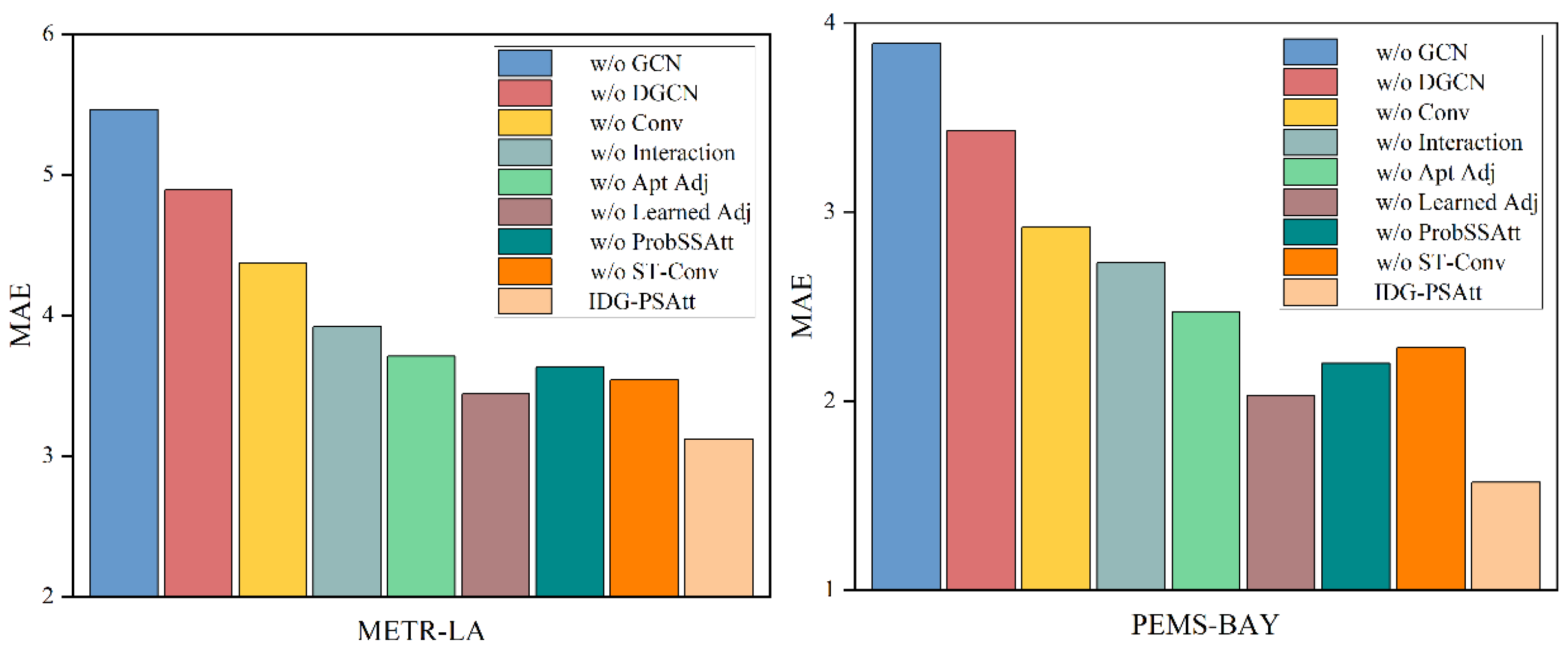
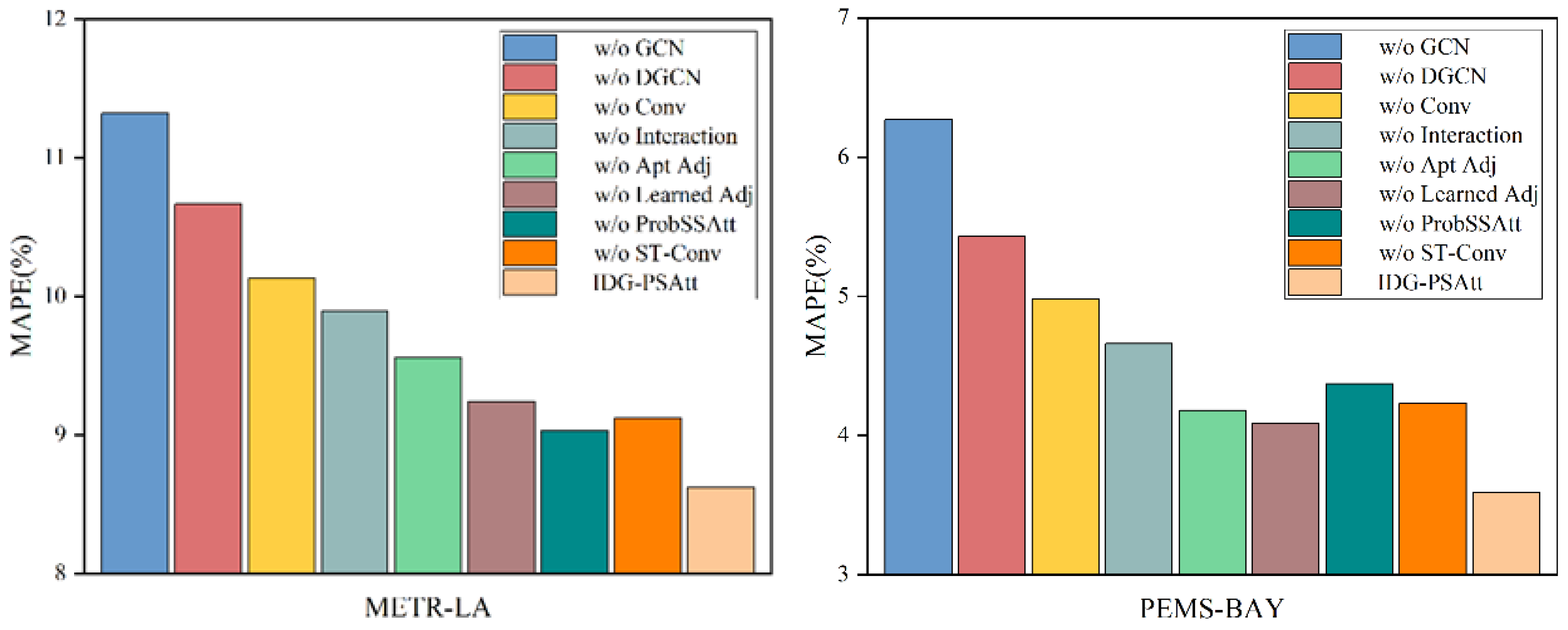
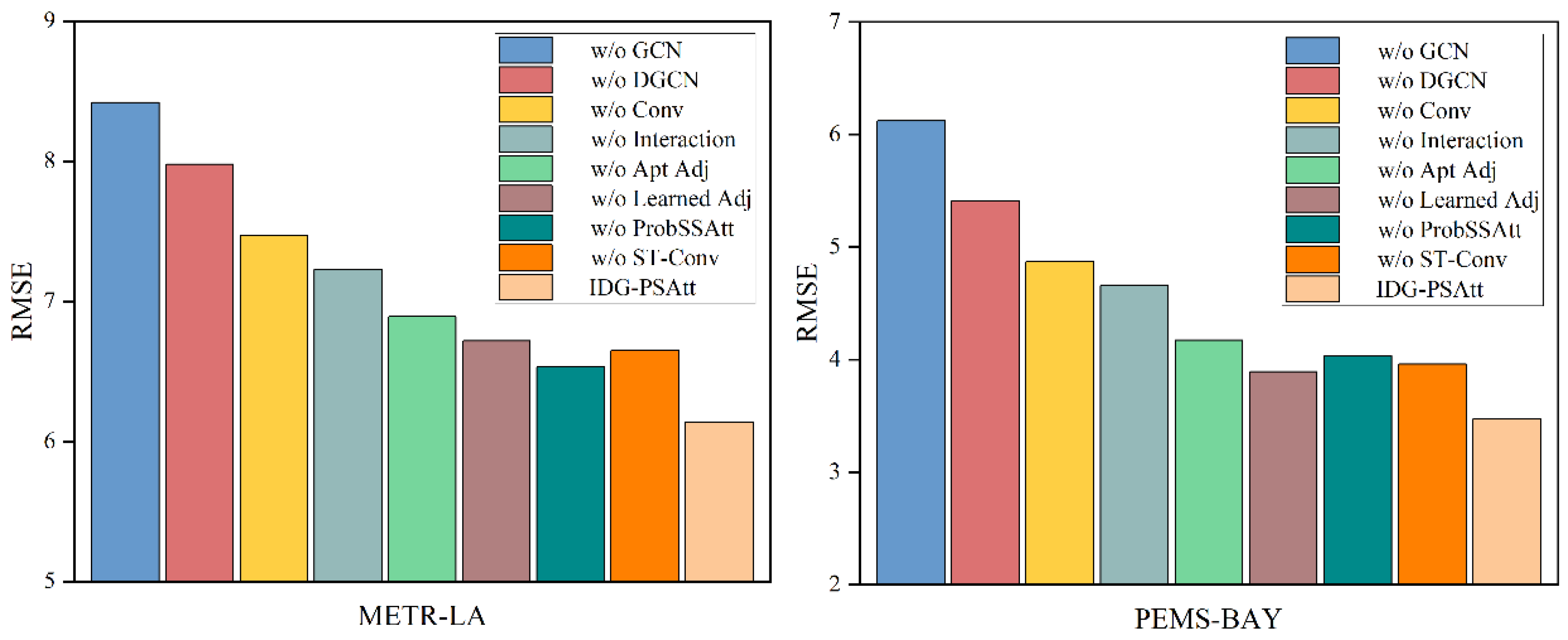
To further investigate the performance of the various modules in the IDG-PSAtt model proposed in this paper, eight variants of the IDG-PSAtt model are designed to verify the effect of each module on the IDG-PSAtt model. These eight variants are compared with the full IDG-PSAtt model in terms of the mean values of the MAE, the RMSE, and the MAPE metrics produced on the METR-LA and the PEMS-BAY datasets, and the results of the ablation experiments are shown in Table 3.
The differences between these eight model variants and the IDG-PSAtt model are as follows:
(1)
GCN w/o: Based on the IDG-PSAtt model, the GCN is removed.
(2)
DGCN w/o: Based on the IDG-PSAtt model, the DGCN is removed.
(3)
Conv w/o: The one-dimensional convolutional modules are removed from the interactive learning structures based on the IDG-PSAtt model.
(4)
Interaction w/o: Based on the IDG-PSAtt model, the interactive learning structures are removed.
(5)
Apt Adj w/o: Based on the IDG-PSAtt model, the adaptive adjacency matrix in the DGCN is removed.
(6)
Learned Adj w/o: Based on the IDG-PSAtt model, the graph generation structure is removed, and the adaptive adjacency matrix is retained.
(7)
ProbSSAtt w/o: Based on the IDG-PSAtt model, the ProbSSAtt block module is removed.
(8)
ST-Conv Block w/o: Based on the IDG-PSAtt model, the ST-Conv module is removed.
The ProbSSAtt and IL-DGCN modules used in this research are essential for improving the performance of the model. As a crucial part of the interactive learning framework, the receptive field is extended using one-dimensional convolution, and ablation tests have shown that one-dimensional convolution can greatly boost the performance of models. Along with the ablation of the two adjacency matrices defined within the DGCN module, the validity of the adaptive adjacency matrix is also investigated in the IDG-PSAtt model, as shown in Figure 5. The dynamic adjacency matrix is created by combining a learnable adjacency matrix with an adaptive adjacency matrix. The dynamic adjacency matrix enables the graph convolution process to more accurately depict the hidden spatial correlations in traffic data, as shown in Table 2 and Figure 5, Figure 6 and Figure 7, demonstrating the effectiveness of the two vital structures proposed in this paper, namely, interactive learning and dynamic graph convolution.
(2)
Visual Analysis
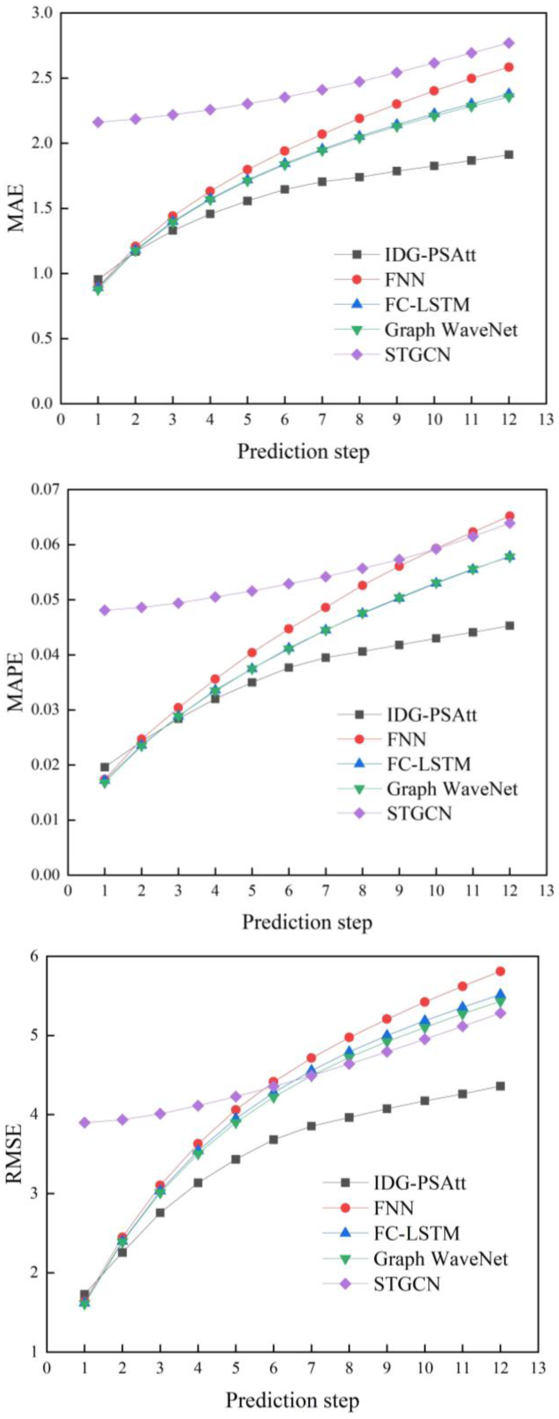
To better explain the proposed IDG-PSAtt model, the experimental outcomes yielded by the IDG-PSAtt, FNN, FC-LSTM, Graph WaveNet, and STGCN models on the PEMS-BAY dataset are visualized in Figure 8. It is obvious from the three subfigures that the prediction performance of the IDG-PSAtt model far exceeds that of the FNN, FC-LSTM, Graph WaveNet, and STGCN models, demonstrating that the proposed model can more adequately extract the dynamic spatial–temporal characteristics of traffic flows. Moreover, as the prediction duration increases, the growth rate of prediction error decreases, and when the prediction duration is longer than 15 min, the prediction errors of IDG-PSAtt are all significantly lower than those of the other comparative models, which indicates that the long-term prediction performance of this model is superior to that of the other models.
The above study reveals that the IDG-PSAtt model yields the best prediction results at different prediction time points. The IDG-PSAtt model accurately predicts traffic congestion, captures the trends of traffic flows, and identifies the starting and ending times of the peak traffic flow period, which proves the excellent prediction performance of the IDG-PSAtt model in the traffic flow prediction task, as well as its effectiveness in real-time traffic prediction. The traffic flow prediction model proposed in this paper can guide transportation planning, thus improving the transportation environment, enhancing the quality of residents’ travel, and promoting the sustainable development of cities.
By accurately predicting traffic flow and congestion, traffic planners can formulate more effective traffic management strategies, such as adjusting signal timing, optimizing route planning, and providing real-time traffic information, among others. These measures not only reduce traffic congestion and improve traffic efficiency, but also enhance the traffic environment. Furthermore, the improved accuracy of real-time traffic flow prediction enabled by the model facilitates the forecasting of mobile source emissions, significantly enhancing the precision of local air quality predictions. This comprehensive approach contributes to both smoother traffic flow and a better environmental outcome [39,40]. This, in turn, can offer valuable data and technical support to environmental management departments to develop various control measures, such as implementing truck bans around a city, restricting the national use of three vehicles, and granting preferential road rights to vehicles using new energy. Furthermore, traffic flow simulations can provide early warnings of potential traffic congestion, enabling the timely implementation of diversionary measures to mitigate emissions resulting from idling vehicles.

4. Conclusions

This paper proposes an efficient and accurate traffic prediction model called IDG-PSAtt, which not only considers non-Euclidean traffic flows but also combines an interactive learning strategy with ST-Conv and ProbSSAtt blocks to fully capture the dynamic spatial–temporal features of traffic flows. This approach solves the problems faced by the noninteractive, previously developed models, which insufficiently capture spatial–temporal features and have difficulty making long-term predictions. Specifically, the IDG-PSAtt model creates a dynamic graph structure by adapting the input spatial–temporal information and employs a preset initial adjacency matrix to simulate the dynamic relationships between nodes for exploring the dynamic associations between the invisible nodes in a traffic network and capturing their hidden spatial correlations. Moreover, an IL-DGCN is constructed by embedding a DGCN block into the interactive learning framework to learn the periodic characteristics and trends of traffic flows and simultaneously capture their spatial–temporal dependencies. Finally, ST-Conv and ProbSSAtt blocks are used to fully exploit the dynamic spatial–temporal features of traffic flows to achieve improved traffic flow prediction accuracy. The IDG-PSAtt model has significantly better prediction performance than the baseline models according to experiments conducted on two traffic datasets. On METR-LA, the MAE and RMSE of IDG-PSAtt for 60 min predictions are reduced by 0.75 and 1.31, respectively, compared with those of the state-of-the-art models. As the training time increases, the performance of the proposed model improves, increasing the accuracy of the predicted traffic flow and the predictability of the traffic flow over the medium-to-long term.
Different cities may have different data collection techniques and standards, so models need to be able to adapt to data from different sources and formats. For example, some cities may need to focus more on the impact of public transportation, while others may need to pay more attention to the flow of private vehicles. Therefore, the IDG-PSAtt model would need to incorporate more variable factors for discussion.
In practical scenarios, external variables such as weather conditions and current social events significantly impact traffic flow prediction tasks. By accounting for these external effects, we can enhance the accuracy and training performance of predictive models. Moreover, environmental protection is a crucial consideration in this context. Accurately forecasting traffic volumes and congestion patterns allows for better traffic management strategy planning, thereby reducing the environmental pollution and energy waste resulting from traffic congestion. Therefore, future research should focus on incorporating environmental protection factors into traffic prediction models to develop more sustainable and eco-friendly transportation systems.

Author Contributions

Conceptualization, H.Y.; methodology, Z.H. (Zhihui Huang); formal analysis, Z.D.; data curation, Z.H. (Zhihui Huang) and Z.D.; writing—original draft, Z.D.; writing—review and editing, Z.H. (Zhuoshi He), visualization, Z.H. (Zhuoshi He) and Z.D.; supervision, J.W. All authors have read and agreed to the published version of the manuscript.

Funding

This work was supported by National Key Research and Development Program of China (No. 2022YFC3703604).

Data Availability Statement

The data presented in this study are available on request from the corresponding author. The data are not publicly available due to privacy.

Conflicts of Interest

The authors declare no conflicts of interest.

Abbreviations

IDG-PSAttinteractive dynamic spatial–temporal graph convolutional probabilistic sparse attention mechanism
IL-DGCNinteractive dynamic graph convolutional network
ST-Convspatial–temporal convolution
ProbSSAttprobabilistic sparse self-attention
GCNgraph convolutional network
MAEmean absolute error
RMSEroot mean square error
ITSsintelligent transportation systems
STGCNspatial–temporal graph convolutional network
GLUsgated linear units
TCNstemporal convolutional networks
GRUgated recursive unit
RNNartificial neural network
MLPmultilayer perceptron
MAPEmean absolute percentage error
HAhistorical average
VARvector autoregression
SVMsupport vector machine
FNNfeedforward neural network
ARIMAAutoregressive Integrated Moving Average Model
FC-LSTMFully Connected Long Short-Term Memory
STGCNSpatiotemporal Graph Convolutional Network
ASTGCNAttention-based Spatial–Temporal Graph Convolutional Network
STSGCNSpatiotemporal Stream Graph Convolutional Network
Nomenclature
G = V , E , A graph
V = N the set of nodes
E the set of edges between the nodes
A N × N denotes the initial adjacency matrix generated by the graph G
A adjacency matrix
X G t + 1 , X G t + 2 , , X G t + T future traffic flows
X G t T + 1 , X G t T + 2 , , X G t historical time series
X G t N × C denotes the observation value of graph G at time t
C denotes the number of feature channels
T denotes the length of the given historical time series
T denotes the length of the predicted future traffic series

References

  1. He, R.; Xiao, Y.; Lu, X.; Zhang, S.; Liu, Y. ST-3DGMR: Spatio-temporal 3D grouped multiscale ResNet network for region-based urban traffic flow prediction. Inf. Sci. 2023, 624, 68–93. [Google Scholar] [CrossRef]
  2. Li, D.; Lasenby, J. Spatiotemporal Attention-Based Graph Convolution Network for Segment-Level Traffic Prediction. IEEE Trans. Intell. Transp. Syst. 2022, 23, 8337–8345. [Google Scholar] [CrossRef]
  3. Wu, Z.; Pan, S.; Long, G.; Jiang, J.; Zhang, C. Graph WaveNet for Deep Spatial-Temporal Graph Modeling. arXiv 2019, arXiv:1906.00121. [Google Scholar] [CrossRef]
  4. Zhang, Q.; Chang, J.; Meng, G.; Xiang, S.; Pan, C. Spatio-temporal graph structure learning for traffic forecasting. In Proceedings of the AAAI Conference on Artificial Intelligence, New York, NY, USA, 7–12 February 2020; Volume 34, pp. 1177–1185. [Google Scholar] [CrossRef]
  5. Shao, Y.; Zhao, Y.; Yu, F.; Zhu, H.; Fang, J. The Traffic Flow Prediction Method Using the Incremental Learning-Based CNN-LTSM Model: The Solution of Mobile Application. Mob. Inf. Syst. 2021, 2021, 5579451. [Google Scholar] [CrossRef]
  6. Li, M.; Zhu, Z. Spatial-temporal fusion graph neural networks for traffic flow forecasting. In Proceedings of the AAAI Conference on Artificial Intelligence, Online, 2–9 February 2021; Volume 35, pp. 4189–4196. [Google Scholar] [CrossRef]
  7. Zhang, T.; Zhang, D.G.; Yan, H.R.; Qiu, J.N.; Gao, J.X. A new method of data missing estimation with FNN-based tensor heterogeneous ensemble learning for internet of vehicle. Neurocomputing 2021, 420, 98–110. [Google Scholar] [CrossRef]
  8. Qi, J.; Zhao, Z.; Tanin, E.; Cui, T.; Nassir, N.; Sarvi, M. A Graph and Attentive Multi-Path Convolutional Network for Traffic Prediction. IEEE Trans. Knowl. Data Eng. 2022, 35, 6548–6560. [Google Scholar] [CrossRef]
  9. Guo, S.; Lin, Y.; Wan, H.; Li, X.; Cong, G. Learning Dynamics and Heterogeneity of Spatial-Temporal Graph Data for Traffic Forecasting. IEEE Trans. Knowl. Data Eng. 2021, 34, 5415–5428. [Google Scholar] [CrossRef]
  10. Bai, L.; Yao, L.; Li, C.; Wang, X.; Wang, C. Adaptive graph convolutional recurrent network for traffic forecasting. Adv. Neural Inf. Process. Syst. 2020, 33, 17804–17815. [Google Scholar] [CrossRef]
  11. Fu, R.; Zhang, Z.; Li, L. Using LSTM and GRU neural network methods for traffic flow prediction. In Proceedings of the 2016 31st Youth Academic Annual Conference of Chinese Association of Automation (YAC), Wuhan, China, 11–13 November 2016; IEEE: Piscataway, NJ, USA, 2016. [Google Scholar] [CrossRef]
  12. Chen, W.; Chen, L.; Xie, Y.; Cao, W.; Gao, Y.; Feng, X. Multirange attentive bicomponent graph convolutional network for traffic forecasting. In Proceedings of the AAAI Conference on Artificial Intelligence, New York, NY, USA, 7–12 February 2020; Volume 34, pp. 3529–3536. [Google Scholar] [CrossRef]
  13. Dong, C.; Shao, C.; Li, X. Short-Term Traffic Flow Forecasting of Road Network Based on Spatial-Temporal Characteristics of Traffic Flow. In Proceedings of the World Congress on Computer Science & Information Engineering, Los Angeles, CA, USA, 31 March–2 April 2009; IEEE: Piscataway, NJ, USA, 2009. [Google Scholar] [CrossRef]
  14. Shi, Z.; Zhang, Y.; Wang, J.; Qin, J.; Liu, X.; Yin, H.; Huang, H. DAGCRN: Graph convolutional recurrent network for traffic forecasting with dynamic adjacency matrix. Expert Syst. Appl. 2023, 227, 120259. [Google Scholar] [CrossRef]
  15. Wu, Z.; Pan, S.; Long, G.; Jiang, J.; Chang, X.; Zhang, C. Connecting the dots: Multivariate time series forecasting with graph neural networks. In Proceedings of the 26th ACM SIGKDD International Conference on Knowledge Discovery & Data Mining, Online, CA, USA, 6–10 July 2020; pp. 753–763. [Google Scholar] [CrossRef]
  16. Song, C.; Lin, Y.; Guo, S.; Wan, H. Spatial-temporal synchronous graph convolutional networks: A new framework for spatial-temporal network data forecasting. In Proceedings of the AAAI Conference on Artificial Intelligence, New York, NY, USA, 7–12 February 2020; Volume 34, pp. 914–921. [Google Scholar] [CrossRef]
  17. Chen, Y.; Wang, W.; Chen, X.M. Bibliometric methods in traffic flow prediction based on artificial intelligence. Expert Syst. Appl. 2023, 228, 120421. [Google Scholar] [CrossRef]
  18. Huo, G.; Zhang, Y.; Wang, B.; Gao, J.; Hu, Y.; Yin, B. Hierarchical Spatio–Temporal Graph Convolutional Networks and Transformer Network for Traffic Flow Forecasting. IEEE Trans. Intell. Transp. Syst. 2023, 24, 3855–3867. [Google Scholar] [CrossRef]
  19. Wang, S.; Pan, Y.; Zhang, J.; Zhou, X.; Cui, Z.; Hu, G.; Pan, Z. Robust and label efficient bi-filtering graph convolutional networks for node classification. Knowl.-Based Syst. 2021, 224, 106891. [Google Scholar] [CrossRef]
  20. Yu, W.; Huang, X.; Qiu, Y.; Zhang, S.; Chen, Q. GSTC-Unet: A U-shaped multi-scaled spatiotemporal graph convolutional network with channel self-attention mechanism for traffic flow forecasting. Expert Syst. Appl. 2023, 232, 120724. [Google Scholar] [CrossRef]
  21. Deng, L.; Zhang, X.; Tao, S.; Zhao, Y.; Wu, K.; Liu, J. A spatiotemporal graph convolution-based model for daily runoff prediction in a river network with non-Euclidean topological structure. Stoch. Environ. Res. Risk Assess. 2023, 37, 1457–1478. [Google Scholar] [CrossRef]
  22. Yan, B.; Wang, G.; Yu, J.; Jin, X.; Zhang, H. Spatial-Temporal Chebyshev Graph Neural Network for Traffic Flow Prediction in IoT-Based ITS. IEEE Internet Things J. 2022, 9, 9266–9279. [Google Scholar] [CrossRef]
  23. Tang, S.; Li, B.; Yu, H. ChebNet: Efficient and Stable Constructions of Deep Neural Networks with Rectified Power Units using Chebyshev Approximations. arXiv 2019, arXiv:1911.05467. [Google Scholar] [CrossRef]
  24. Cui, Z.; Ke, R.; Pu, Z.; Wang, Y. Stacked bidirectional and unidirectional LSTM recurrent neural network for forecasting network-wide traffic state with missing values. Transp. Res. Part C Emerg. Technol. 2020, 118, 102674. [Google Scholar] [CrossRef]
  25. Fukuda, S.; Uchida, H.; Fujii, H.; Yamada, T. Short-term Prediction of Traffic Flow under Incident Conditions using Graph Convolutional RNN and Traffic Simulation. IET Intell. Transp. Syst. 2020, 14, 936–946. [Google Scholar] [CrossRef]
  26. Liang, G.; Kintak, U.; Tiwari, P.; Nowaczyk, S.; Kumar, N. Semantics-Aware Dynamic Graph Convolutional Network for Traffic Flow Forecasting. IEEE Trans. Veh. Technol. 2023, 72, 7796–7809. [Google Scholar] [CrossRef]
  27. Chen, Z.; Lu, Z.; Chen, Q.; Zhong, H.; Zhang, Y.; Xue, J.; Wu, C. Spatial-temporal short-term traffic flow prediction model based on dynamical-learning graph convolution mechanism. Inf. Sci. 2022, 611, 522–539. [Google Scholar] [CrossRef]
  28. Xu, Y.; Cai, X.; Wang, E.; Liu, W.; Yang, Y.; Yang, F. Dynamic traffic correlations based spatio-temporal graph convolutional network for urban traffic prediction. Inf. Sci. 2023, 621, 580–595. [Google Scholar] [CrossRef]
  29. Zheng, G.; Chai, W.K.; Katos, V. A dynamic spatial-temporal deep learning framework for traffic speed prediction on large-scale road networks. Expert Syst. Appl. 2022, 195, 116585. [Google Scholar] [CrossRef]
  30. Zheng, C.; Fan, X.; Wang, C.; Qi, J. Gman: A graph multi-attention network for traffic prediction. In Proceedings of the AAAI Conference on Artificial Intelligence, New York, NY, USA, 7–12 February 2020; pp. 1234–1241. [Google Scholar] [CrossRef]
  31. Khaled, A.; Elsir, A.M.T.; Shen, Y. TFGAN: Traffic forecasting using generative adversarial network with multi-graph convolutional network. Knowl. Based Syst. 2022, 249, 108990. [Google Scholar] [CrossRef]
  32. Huang, B.; Dou, H.; Luo, Y.; Li, J.; Wang, J.; Zhou, T. Adaptive Spatiotemporal Transformer Graph Network for Traffic Flow Forecasting by IoT Loop Detectors. IEEE Internet Things J. 2023, 10, 15. [Google Scholar] [CrossRef]
  33. Liu, Q.; Wang, B.; Zhu, Y. Shor-term Traffic Speed Forecasting Based on Attention Convolutional Neural Network for Arterials. Comput.-Aided Civ. Infrastruct. Eng. 2018, 33, 999–1016. [Google Scholar] [CrossRef]
  34. Divyam, S.A.; Singh, B. Comparative Study of Static VAR Compensation Techniques—Thyristor Switched Reactor and Thyristor Switched Capacitor. In Proceedings of the International Conference on Communication and Electronics Systems, Coimbatore, India, 10–12 June 2020. [Google Scholar] [CrossRef]
  35. Wu, Y.; Tan, H. Short-term traffic flow forecasting with spatial-temporal correlation in a hybrid deep learning framework. arXiv 2016, arXiv:1612.01022. [Google Scholar] [CrossRef]
  36. Yan, H.; Ma, X.; Pu, Z. Learning dynamic and hierarchical traffic spatiotemporal features with transformer. IEEE Trans. Intell. Transp. Syst. 2021, 23, 22386–22399. [Google Scholar] [CrossRef]
  37. Ishida, K.; Ercan, A.; Nagasato, T.; Kiyama, M.; Amagasaki, M. Use of 1D-CNN for input data size reduction of LSTM in Hourly Rainfall-Runoff modeling. arXiv 2021, arXiv:2111.04732. [Google Scholar] [CrossRef]
  38. Rio, J.; Momey, F.; Ducottet, C.; Alata, O. WaveNet based architectures for denoising periodic discontinuous signals and application to friction signals. In Proceedings of the 2020 28th European Signal Processing Conference (EUSIPCO), Amsterdam, The Netherlands, 18–21 January 2021; pp. 1580–1584. [Google Scholar] [CrossRef]
  39. Chen, J.; Yu, Y.; Guo, Q. Freeway traffic congestion reduction and environment regulation via model predictive control. Algorithms 2019, 12, 220. [Google Scholar] [CrossRef]
  40. Medina-Salgado, B.; Sánchez-DelaCruz, E.; Pozos-Parra, P.; Sierra, J.E. Urban traffic flow prediction techniques: A review. Sustain. Comput. Inform. Syst. 2022, 35, 100739. [Google Scholar] [CrossRef]
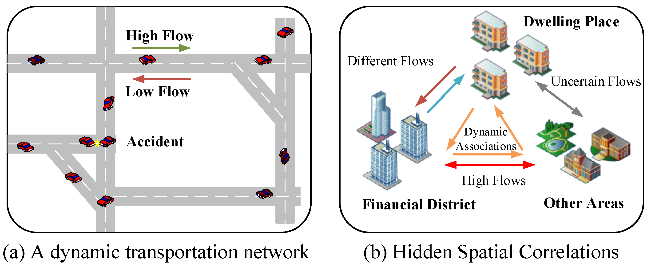
Figure 1. Dynamic spatial–temporal correlations of traffic flows.
Atmosphere 15 00413 g001
Figure 2. Structure of an STGCN.
Atmosphere 15 00413 g002
Figure 3. Overall framework of IDG-PSAtt.
Atmosphere 15 00413 g003
Figure 4. Diagram of the ST-Conv block framework.
Atmosphere 15 00413 g004
Figure 5. Comparison between the MAE metrics produced on the two datasets.
Atmosphere 15 00413 g005
Figure 6. Comparison between the MAPE metrics produced on the two datasets.
Atmosphere 15 00413 g006
Figure 7. Comparison between the RMSE metrics produced on the two datasets.
Atmosphere 15 00413 g007
Figure 8. Visualizations of the comparisons conducted between different models on the PEMS-BAY dataset.
Atmosphere 15 00413 g008
Table 1. Description of the experimental datasets.
DataMETR-LAPEMS-BAY
Typesequentialsequential
Attributespeedspeed
Locationhighways of Los Angelesthe Bay Area
Edges15152369
Time Steps34,27252,116
Nodes207325
Table 2. Comparison between IDG-PSAtt and the baselines on two traffic datasets.
DataModels15 min30 min60 min
MAERMSEMAPEMAERMSEMAPEMAERMSEMAPE
METR-LAHA4.568.9213.00%4.568.9213.00%4.568.9213.00%
VAR4.427.8910.20%5.419.1312.7%6.5210.1115.80%
SVR3.998.459.30%5.0510.8712.10%6.7213.7616.70%
FNN3.997.949.90%4.238.1712.90%4.498.6914.00%
ARIMA3.998.219.60%5.1510.4512.70%6.9013.2317.40%
FC-LSTM3.446.309.60%3.777.2310.90%4.378.6913.20%
WaveNet2.995.898.04%3.597.2810.25%4.458.9313.62%
GWN2.985.907.92%3.597.2910.26%4.438.9713.64%
STGCN2.885.747.62%3.477.249.57%4.599.4012.70%
ASTGCN4.869.279.21%5.4310.6110.13%6.5112.5211.64%
STSGCN3.317.628.06%4.139.7710.29%5.0611.6612.91%
IDG-PSAtt2.775.287.24%3.156.248.73%3.627.3810.52%
PEMS-BAYHA2.885.596.80%2.885.596.80%2.885.596.80%
VAR1.743.163.60%2.324.255.00%2.935.446.50%
SVR1.853.593.80%2.485.185.50%3.287.088.00%
FNN2.204.425.19%2.304.635.43%2.464.985.89%
ARIMA1.623.303.50%2.334.765.40%3.386.508.30%
FC-LSTM2.054.194.80%2.204.555.20%2.374.965.70%
WaveNet1.393.012.91%1.834.214.16%2.355.435.87%
GWN1.393.012.89%1.834.214.11%2.355.435.78%
STGCN1.362.962.90%1.814.274.17%2.495.695.79%
ASTGCN1.523.133.22%2.014.274.48%2.615.426.00%
STSGCN1.443.013.04%1.834.184.17%2.265.215.40%
IDG-PSAtt0.961.721.96%1.643.683.77%1.914.364.53%
Table 3. Comparison between IDG-PSAtt and its variants on two traffic datasets.
DatasetModelMAERMSEMAPE
METR-LAw/o GCN5.468.4211.32%
w/o DGCN4.897.9810.67%
w/o Conv4.377.4710.13%
w/o Interaction3.927.239.89%
w/o Apt Adj3.716.899.56%
w/o Learned Adj3.446.729.24%
w/o ProbSSAtt3.636.539.03%
w/o ST-Conv3.546.659.12%
IDG-PSAtt3.126.148.62%
PEMS-BAYw/o GCN3.896.126.27%
w/o DGCN3.435.415.43%
w/o Conv2.924.874.98%
w/o Interaction2.734.664.66%
w/o Apt Adj2.474.174.18%
w/o Learned Adj2.033.894.09%
w/o ProbSSAtt2.204.034.37%
w/o ST-Conv2.283.964.23%
IDG-PSAtt1.573.473.59%
Disclaimer/Publisher’s Note: The statements, opinions and data contained in all publications are solely those of the individual author(s) and contributor(s) and not of MDPI and/or the editor(s). MDPI and/or the editor(s) disclaim responsibility for any injury to people or property resulting from any ideas, methods, instructions or products referred to in the content.