Computational Fluid Dynamics-Based Calculation of Aerosol Transport in a Classroom with Window Ventilation, Mechanical Ventilation and Mobile Air Purifier

Abstract

During the SARS-CoV-2 pandemic, the air quality and infection risk in classrooms were the focus of many investigations. Despite general recommendations for sufficient ventilation, quantitative analyses were often lacking due to the large number of combinations of boundary conditions. Hence, in this paper, we describe a computational fluid dynamics model that predicts the time-resolved airflow for a typical 45 $\min$ classroom scenario. We model 28 students and a teacher, each emitting CO₂ and an individual aerosol. We investigated 13 ventilation setups with window or mechanical ventilation and different positions and operating conditions of an additional air purifier. The ventilation performance is assessed by evaluating the ventilation effectiveness, aerosol removal effectiveness, local air exchange efficiency and overall inhaled aerosol mass of the occupants, which is a measure of the infection risk. If the window is opened according to the “20-5-20” recommendation, the incoming airflow reduces both the CO₂ and aerosol concentration whilst decreasing the thermal comfort at low ambient temperatures. An active air purifier enhances aerosol removal, but, depending on the position, the local air exchange efficiency and individual aerosol inhalation vary. If mechanical ventilation with 700 m³/h is utilised, the CO₂ concentration is kept below 1250 ppm while also effectively removing aerosol from the classroom.

1. Introduction

During the SARS-CoV-2 pandemic, the virus mainly spread within insufficiently ventilated indoor environments. The prominent case described by Lu et al. [1], where the virus was spread by the air conditioning system in a restaurant, emphasises not only the need for an overall sufficient ventilation rate but also the requirement of an overall good distribution of fresh air. Public spaces like restaurants or cinemas were widely shut down, but since schools had to stay open as long as possible, the indoor environment of classrooms became an intensively discussed topic. To enable a safe environment within classrooms that prevented the uncontrolled spread of the virus, several institutions and authors analysed case studies and developed models and/or tools to assess the infection risk and derive measures to allow the normal operation of schools.

One reported case of infection within a classroom setting was described by Lam-Hine et al. [2]. In an elementary school, half of the students were infected by the symptomatic teacher. The teacher and the students did not wear face masks, but a mobile air purifier was operated.

Many researchers developed models to predict the risk of infection [3,4,5,6,7]. Müller et al. [4] developed a simplified calculation approach to determine a relative infection risk from aerosol-borne viruses in indoor environments. They assume a reference scenario for which an absolute infection risk was derived based on various approaches as known from the present literature. Using this reference scenario as a baseline, a relative infection risk can be computed for various other scenarios. The calculation was compared to the results of other tools [7,8,9].

The German Federal Environment Agency (UBA) published a handout where they proposed natural ventilation as a measure to reduce the risk of infection, especially in the context of classrooms [10]. They also note that mobile air purifiers are viable add-on measures to further reduce the infection risk. The Center for Disease Control and Prevention (CDC) suggests a minimum of five air changes per hour [11] but does not further specify how this is best achieved. A similar recommendation is given by the Chinese Center for Disease Control and Prevention (CCDC), as they suggest a minimum fresh air rate of 30 ${\mathrm{m}}^3$/$\mathrm{h}$ per person [12]. If this lower limit can not be sustained, the number of occupants in the room has to be reduced.

Lowther et al. [13] rated the removal efficiency of selected air purifiers regarding different particle size distributions. Overall, they observed higher removal efficiencies at higher volume flow rates. Curtius et al. [14] investigated the filtration behaviour of mobile air purifiers in a closed classroom setting. They observed a significant reduction in inhaled particle doses when operating the mobile air purifier at high volume flow rates. In their study, Jain et al. [15] investigate a classroom setting where a large air purifier is operated at different positions and volume flow rates. Under the assumption of steady-state conditions, neglecting any transient effects, they calculate an infection risk originating from varying index patients. They observed an overall reduction in the infection risk in all investigated scenarios where the air purifier was active, although zones with high local concentrations were found. Assuming different heating settings in a small chamber, Sabanskis et al. [16] confirmed the strong sensitivity of the filtering efficiency of a mobile air purifier to the positions of both the aerosol source and the filtration device. Duill et al. [17] conducted a thorough study to investigate a classroom setting using different air purifier types, with one type operated at two different locations. The classroom was additionally ventilated following the guidelines from the UBA [10]. They were able to show that mobile air purifiers can significantly reduce aerosol concentrations. A developed flow model was able to predict the aerosol decay rate in good agreement with measured data, although it was only validated for periods without window ventilation. At the tested volume flow rates of about 1000 ${\mathrm{m}}^3$/$\mathrm{h}$, the noise of the devices was reported to not negatively impact the learning environment. Fierce et al. [18] performed simulations of a quadrature-based model to predict the spread and inhalation of airborne pathogens. They investigated the influence of the use of face masks and increased ventilation rates. Both measures lead to a significant reduction in droplet inhalation for larger distances away from the droplet source.

Chirico et al. [19] reviewed several reported outbreaks in Asia that had in common that a central ventilation system recirculated at least a portion of the airflow into the rooms. Because the ventilation systems used recirculation air, they captured the infectious particles and distributed them over the whole ventilation system, leading to more infections. In their review, no studies on classrooms were included. Elsaid and Ahmed [20] reviewed current design methods of ventilation systems with a focus on reducing the spread of potentially infectious particles. They recommend operating air handling units such that as much outdoor air as possible is provided into the indoor environment. Furthermore, the air handling units should utilise filters that are capable of effectively removing particles below $0.3$ $\mathsf{\mu }\mathrm{m}$ from the air. In his study, Melikov [21] reviewed a mixing, underfloor and displacement ventilation scenario by conduction tracer gas measurements. He concludes that increasing the ventilation rate utilising mixing ventilation is not always the best way to reduce the infection risk, since it potentially spreads the airborne infection in the room. Using an infection risk to derive the ventilation effectiveness, Kurnitski et al. [22] assess the local air quality using tracer gas measurements. They discuss different room scenarios with varying locations of the point source, which represents an infected person. Across all scenarios, the source location in combination with the position(s) of the extract air ducts strongly impacts the overall distribution of the air quality.

There seems to exist an overall consensus on the fact that a ventilation system utilising recirculation air poses an increased risk of infection. To reduce the infection risk, the same ventilation system can be used if only non-contaminated air, such as fresh outdoor air or cleaned air, is supplied. Since many public facilities, especially German school classrooms, are not equipped with a mechanical ventilation system, only natural ventilation or mobile air purifiers are available to lower the infection risk. As most air purifiers do not filter human CO₂ emissions, their usage without additional ventilation is not advisable or purposeful regarding indoor air quality. Particularly during the winter season, window ventilation is only utilisable intermittently due to thermal comfort reasons [23]. In contrast, air purifiers can be operated continuously. This may result in transient progressions of pollutant concentrations during a school lesson. In addition, there are different thermal buoyancy effects to be considered inside a classroom due to heat sources, such as students and teachers, radiators and lamps, and further thermal effects due to the unconditioned outdoor air caused by window ventilation. Under these aspects, it can be assumed that inhomogeneous and transient pollutant concentrations may be present under the operation of air purifiers and window ventilation in classrooms. Under inhomogeneous concentration distributions, the position of the air purifier in the classroom can have an important impact on effectiveness [17]. Thus, to accurately evaluate the effectiveness of air purifiers in filtering potentially infectious particles, both transient and inhomogeneous effects in the room must be considered.

All the discussed studies have in common that they assume steady-state flow conditions. Window ventilation is a strongly transient flow, which is challenging for the descriptions commonly applied to comparable problems. Additional transient effects result from the intermittent use of window ventilation. We introduce a significantly higher number of tracers into our simulation setup, which allows us to reliably derive the uncertainty associated with each investigated scenario. By treating CO₂ as an inert tracer that is not filtered, we can segregate flow behaviour and filtration effectiveness. By using detailed, transient flow simulation models, including window or mechanical ventilation and mobile air purifiers, we aim to derive metrics that describe various effects influencing the inhalation of a potentially infectious aerosol. Besides the ventilation strategy proposed by the UBA, we also assess the influence of different air purifier operation strategies by varying the volume flow rate and air purifier location. In this work, we further extend the investigations from Ostmann et al. [24] by also taking a simplified air handling unit into account.

2. Methods

This section is dedicated to the description of the developed flow model. We will first describe the geometry, the generated computational grid and the used flow models. A detailed discussion of our assumptions regarding energy and species transport is given before we introduce the developed metrics to rate the performance of the proposed ventilation concepts.

The whole model is developed using the software package ANSYS 2020 R2 [25]. We use the associated Design Modeler to design the geometry and then feed it into ANSYS Meshing to generate the computational grid. The setup of the flow model is implemented using the CFX package.

2.1. Description of the Geometry

The geometry of the classroom model is derived from a real scenario [26], and a summary of the geometric parameters is given in

Table 1. Geometric dimensions of the investigated classroom.

Quantity	Value	Unit	Description
$b_{\mathrm{Room}}$	$7.35$	$\mathrm{m}$	Width of the classroom
$h_{\mathrm{Room}}$	3.00	$\mathrm{m}$	Height of the classroom
$l_{\mathrm{Room}}$	$9.52$	$\mathrm{m}$	Length of the classroom
$V_{\mathrm{Room},\mathrm{geom}}$	≈210	${\mathrm{m}}^3$	Geometric volume of the classroom
$V_{\mathrm{Room}}$	$199.92$	${\mathrm{m}}^3$	Effective air volume of the classroom
$b_{\mathrm{Window}}$	$1.86$	$\mathrm{m}$	Width of the windows
$h_{\mathrm{Window}}$	$1.48$	$\mathrm{m}$	Height of the windows
$A_{\mathrm{Window}}$	$2.75$	${\mathrm{m}}^2$	Area of a window
$n_{\mathrm{Window}}$	4	-	No. of windows
$A_{\mathrm{AP}}$	4.70	${\mathrm{m}}^2$	Surface area of an air cleaner

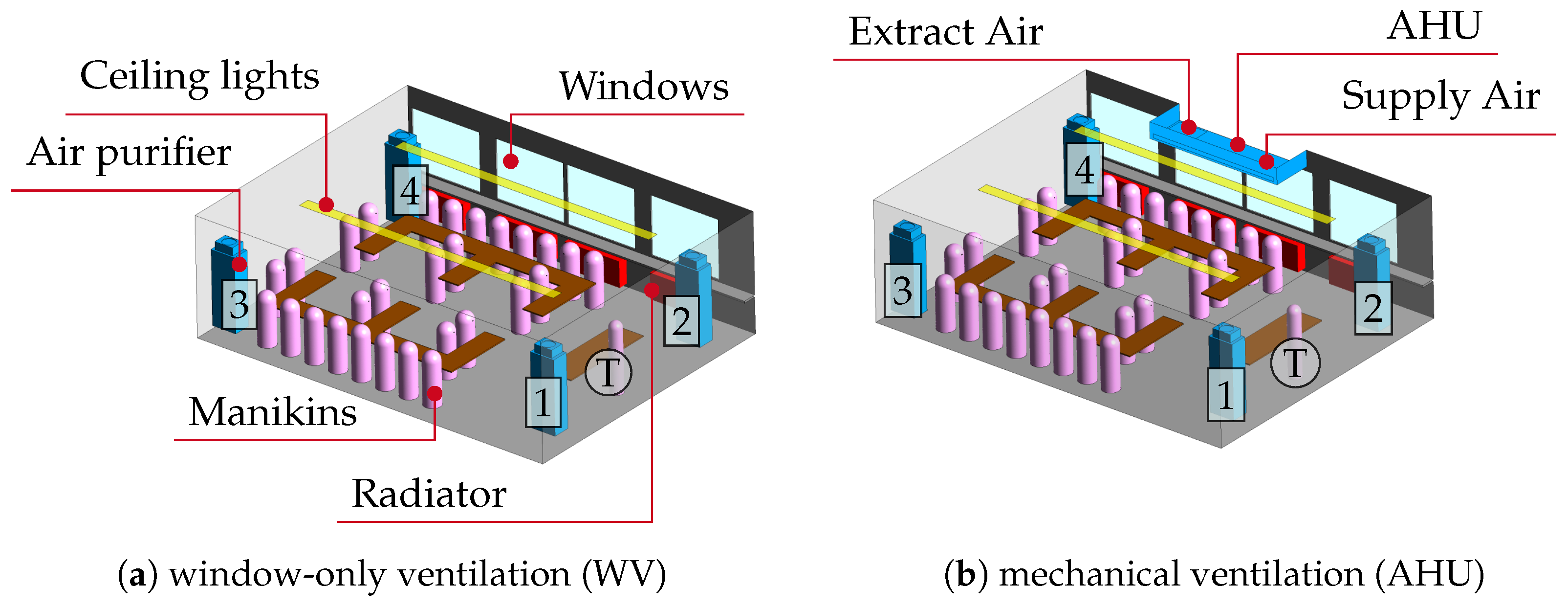
. An overview of the investigated classroom settings is shown in Figure 1. The 28 students and the teacher are modelled as manikins. The geometric volume of the classroom is reduced by the volume of the manikins and the air purifiers to an effective air volume of roughly 200 ${\mathrm{m}}^3$. We treat the desks as solid, adiabatic surfaces. The students are seated in a typical manner, with the mouths of the students being oriented either towards the opposite wall or towards the wall behind the teacher (see Figure 1). The teacher is assumed to be standing facing towards the back wall of the classroom and therefore in the direction of the students. We denote the students using an index in the range $i,j=\left[1,28\right]$, and the teacher is denoted by either the index $i,j=29$ or “T”.

All present occupants are simplified using manikins consisting of a cylindrical base shape with a half-sphere on top according to Menchaca-B. and Leon R. Glicksman [27]. To yield roughly equal surface areas, the seated students feature a height of $1.3$ $\mathrm{m}$ with a diameter of $0.43$ $\mathrm{m}$, and the teacher is $1.75$ $\mathrm{m}$ tall with a diameter of $0.32$ $\mathrm{m}$. Each manikin features a mouth area of $A_{\mathrm{Mouth}}=3 \mathrm{cm}·1 \mathrm{cm}=3 {\mathrm{cm}}^2$, which is located $0.13$ $\mathrm{m}$ below the tip.

Four radiators are located below the window sills. We simplify the radiators using a cuboid volume with a volumetric heat source. We assume a total of ten ceiling lights by dedicating two long surfaces where each surface approximates five lights. The ceiling lights are aligned with the ceiling itself to decrease the mesh complexity.

We propose four possible locations for a mobile air purifier (see Figure 1a) in the corners of the classroom. The air purifier (AP) model is based on a simplified version of a commercially available air purifier of the type “TAP” from the company TROX GmbH TROX TAP (see [28]). We approximate the inlet of the air purifier using a rectangular surface and the outlet using a circular area. For practical reasons regarding the operability of the model, the same geometric setup is used for each air cleaner scenario, and the respective air cleaners are switched on or off only. In consequence, the geometry of all four possible air purifiers is present in all investigated scenarios. However, we estimate the influence of an inactive air purifier to be insignificant if the respective surfaces are treated as adiabatic boundaries. A more detailed geometric description of the air purifier can be found in Ostmann et al. [29].

The classroom features four windows, each representing a two-winged window as per the referenced classroom [26]. The ratio of window area to classroom floor area is roughly 0.157. The window sills protrude into the room by $0.35$ $\mathrm{m}$ and cover the windows from the radiators below.

In addition to purely natural convective ventilation, we also investigate the case of mechanical ventilation with a simplified air handling unit (AHU) (see Figure 1b). The supply air is provided through a long rectangular slot with a flow cross-section of $A_{\mathrm{SUP}}=0.33 {\mathrm{m}}^2$, which covers nearly the whole width of the device. The extract air is drawn through a rectangular opening in the bottom of the device with a cross-section of $A_{\mathrm{ETA}}=0.56 {\mathrm{m}}^2$.

2.2. Computational Flow Model

We use ANSYS Meshing to generate an unstructured tetrahedral volume mesh. To resolve the boundary layer on relevant surfaces, we generate so-called “prism layers”. A section through the whole computational grid of the classroom is shown in Figure 2, where the most relevant features of the flow model are highlighted. We set an average grid resolution of $\Delta x=0.1 \mathrm{m}$ but implement certain refinements to capture the relevant flow structures. A summary of the implemented refinements is given in

Table 2. Parameters that describe the mesh refinements.

Surface/Volume	$\Delta {\mathit{x}}_{\mathbf{Refinement}}$	${\mathit{r}}_{\mathbf{Influence}}$
Manikins	$2.0\times {10}^{-2}$ $\mathrm{m}$	-
Mouth areas	$2.5\times {10}^{-3}$ $\mathrm{m}$	$1\times {10}^{-2}$ $\mathrm{m}$
Ceiling lights	$5.0\times {10}^{-2}$ $\mathrm{m}$	$1\times {10}^{-1}$ $\mathrm{m}$
Air purifiers	$5.0\times {10}^{-2}$ $\mathrm{m}$	$4\times {10}^{-1}$ $\mathrm{m}$
Radiators	$5.0\times {10}^{-2}$ $\mathrm{m}$	-

. Most of the refinements are implemented as surface refinements, where the resulting surface mesh is refined to $\Delta x_{\mathrm{Refinement}}$. To increase the influence of the refined surface mesh into the volume mesh, a certain influence radius $r_{\mathrm{Influence}}$ is specified. As already described, the radiators are simplified as volumes, which is why we use volumetric refinement to properly resolve the heat sources. The resulting mesh consists of roughly 2.4 × 10⁶ cells.

To properly capture the heat transfer from heated surfaces, it is crucial to resolve the airflow boundary layer by implementing several prism layers. Figure 3 shows the prism layer distribution on the surface of a manikin.

To fully describe the prism layers, three parameters (the first layer height, number of layers and growth ratio) are needed. The first layer height $h_1$ describes the height of the first prism layer on the surface and is required by the turbulence model to assess the wall regime and select the appropriate wall function. Based on the first layer height, the remaining prism layers are constructed using the height of the preceding layer $h_i$ and a growth rate factor $f_{\mathrm{Growth}}$ according to Equation (1).

$$h_{i+1}=h_i·f_{\mathrm{Growth}}$$

(1)

In

Table 3. Parameters of the generated prism layers on the respective surfaces.

Surface	${\mathit{h}}_1$	${\mathit{n}}_{\mathbf{Layers}}$	${\mathit{f}}_{\mathbf{Growth}}$
Manikins	$2\times {10}^{-3}$ $\mathrm{m}$	7	1.2
Windows	$4\times {10}^{-3}$ $\mathrm{m}$	5	1.2
Air purifiers	$4\times {10}^{-3}$ $\mathrm{m}$	5	1.2

, the parameters of the prism layers are given for all surfaces, where we resolve the boundary layer.

We assess the quality of our mesh by conducting a grid independency study according to the procedure described by Celik et al. [30]. To reduce the required computational effort, we compute a steady-state solution with the AP active at location with a volume flow rate of 1400 ${\mathrm{m}}^3$/$\mathrm{h}$. Furthermore, we only consider student to be present. The geometries of all other occupants are included but treated as passive and adiabatic. We iterate the solution for 12,000 steps, which is enough to achieve sufficient convergence when averaging the steady-state solutions over the last 1000 iterations. Apart from the base mesh configuration, we also investigate two additional meshes where we reduce and increase all mesh parameters, including the number and first layer height of prism layers, by a factor of 1.5. This yields a coarser ($1.0\times {10}^6$ cells) and a finer ($6.9\times {10}^6$ cells) computational grid. We evaluate both grid convergence indices ${\mathrm{GCI}}_{\mathrm{base}/\mathrm{fine}}$ for the average classroom temperature ${\overline{T}}_{\mathrm{Room}}$ and the aerosol concentration that is captured by the AP $x_{\mathrm{Aerosol},20,\mathrm{AP}1,\mathrm{in}}$. The average classroom temperature features convergent behaviour as indicated by ${\mathrm{GCI}}_{\mathrm{base}}=3.86\times {10}^{-4}$ and ${\mathrm{GCI}}_{\mathrm{fine}}=2.95\times {10}^{-6}$ and a ratio of ${\epsilon }_{21}/{\epsilon }_{32}=0.13$ (see Figure A1). The deviation ${\epsilon }_{\mathrm{ij}}$ is defined as the difference between the values on the finer grid i and the coarser grid j. Although the captured aerosol mass also features good grid convergence with ${\mathrm{GCI}}_{\mathrm{base}}=4.74\times {10}^{-2}$ and ${\mathrm{GCI}}_{\mathrm{fine}}=4.49\times {10}^{-2}$, the associated order p is significantly lower. The ratio ${\epsilon }_{21}/{\epsilon }_{32}=-2.30$ indicates oscillatory and diverging behaviour (see Figure A2). The overall deviations across the three investigated grids are below 4% compared to the base value. Therefore, we evaluate the resolution of the base grid to be a reasonable tradeoff between accuracy and computational effort.

An overview of the models used is given in

Table 4. Models used in the flow simulation.

Model	Selected
Turbulence	k-$\omega$-SST [33]
Radiation	Discrete transfer radiation [34] with 8 rays (surface to surface)
Fluid	Air as a single-component gas with Boussinesq assumption [35] and gravity
Energy	Thermal energy
Time	Transient

. We model the fluid as air with a constant density of ${\rho }_{\mathrm{Air}}=1.185 \mathrm{k}\mathrm{g}/{\mathrm{m}}^3$. Due to the lower density of warmer air, buoyancy forces arise, which are modelled using the Boussinesq assumption with a reference temperature of 20 °C, assuming sufficiently small temperature variations. The reference temperature matches the surface temperature of the room walls (see Section 2.5.3) and is, therefore, a consistent baseline temperature across all scenarios. Since scale-resolved modelling of the occurring turbulence is very resource-intensive, the turbulence is represented in a simplified way using a two-equation model. In this work, we use the k-$\omega$-SST model, as it performs better at describing the boundary layer very close to walls than the k-$\epsilon$ model [31,32]. We can therefore use the fine grid discretisation of our mesh to model the heat transfer process described in Section 2.5.

2.3. Implementation of Window Ventilation

To accurately model the ventilation behaviour, the classroom’s flow model needs to be extended by an additional volume representing the outdoor environment. Although more simple empirical models describing the flow through open windows exist, they are not suitable to represent the strongly transient and, regarding the window opening area, not uniform behaviour during the investigated window ventilation phase [36]. We model the outdoor environment as a cuboid with the dimensions 10 $\mathrm{m}$ × 16 $\mathrm{m}$ × 6 $\mathrm{m}$ (L × W × H), embodying a total volume of 960 ${\mathrm{m}}^3$, as shown in Figure 4.

All scenarios that feature window ventilation use the same (20/5/20) recommendation strategy proposed by the German Federal Environment Agency [10]. They recommend fully opening the windows for at least 3–5 $\min$ after every 20 $\min$ during a lecture. Therefore, the windows are closed for the first 20 $\min$ of the simulation. Within one simulation step, the windows are fully opened, representing the maximum available cross-section for window ventilation. When opening the windows, we change the window surfaces from a wall boundary condition to an interface connected to the outdoor environment. The outdoor environment is initialised with an air temperature $T_{\mathrm{amb}}$ as specified by the respective scenario and a homogeneous CO₂ concentration equal to $c_{{\mathrm{CO}}_2,\mathrm{ref}}$. We further assume no air movement like wind or gusts in the environment, which could further enhance the air exchange. When closing the windows after an additional 5 $\min$, the window’s surfaces are changed back to wall boundaries and the outdoor environment is neglected again. For the periods where the windows are closed, they are modelled with a constant heat transfer coefficient. This represents a heat loss to the (colder) ambient environment.

To evaluate the effective volume flow rate entering the classroom, we first define our x-direction to be positive in the direction from the outdoor environment into the classroom. Therefore, we define a surface where the velocity in the x-direction is positive ($v_x>0$), representing the section of the window cross-section where air enters the classroom. Using this condition, we develop the expression in Equation (2) that yields the volume flow rate entering the classroom ${\dot{V}}_{\mathrm{Window},\mathrm{in}}$. A similar expression can be developed for the volume flow rate exiting the classroom ${\dot{V}}_{\mathrm{Window},\mathrm{out}}$ by switching the condition for the $k_{\mathrm{direction}}$.

$$\begin{array}{cc}\hfill {\dot{V}}_{\mathrm{Window},\mathrm{in}}=& {\int }^{A_{\mathrm{Window}}}v·k_{\mathrm{direction}}dA\hfill \\ \hfill \mathrm{with}& k_{\mathrm{direction}}=\left\{\begin{array}{cc}1\hfill & v_{\mathrm{x}}>0\hfill \\ 0\hfill & v_{\mathrm{x}}\le 0\hfill \end{array}\right.\hfill \end{array}$$

(2)

To calculate the average volume flow entering the classroom during the window ventilation period over the windows, ${\overline{\dot{V}}}_{\mathrm{Window},\mathrm{in}}$ we average the ${\dot{V}}_{\mathrm{Window},\mathrm{in}}$ from Equation (2) and relate it to the duration of one lesson according to Equation (3).

$${\overline{\dot{V}}}_{\mathrm{Window},\mathrm{in}}=\frac{{\int }_{\tau =20\min }^{25\min }{\dot{V}}_{\mathrm{Window},\mathrm{in}}\left(\tau \right)dt}{45\min }$$

(3)

2.4. Species Transport

Each occupant is assumed to emit CO₂ and an individual aerosol ${\Phi }_i$. The aerosol represents potentially infectious airborne particles and is used to evaluate the effectiveness of ventilation designs or air cleaners. Typically, airborne infections are caused by so-called droplet nuclei, i.e., residues of vaporised droplets and particles from the human respiratory tract. The WHO classifies droplet nuclei as particles with a diameter of less than 5 $\mathsf{\mu }$$\mathrm{m}$ [37]. Laboratory studies show that particles in the sizes from 70 $\mathrm{n}$$\mathrm{m}$ to 5 $\mathsf{\mu }$$\mathrm{m}$ disperse similarly to N₂O tracer gas in indoor air under mixed ventilation conditions [38]. In another study, particles in sizes from 30 $\mathrm{n}$$\mathrm{m}$ to $3.2$ $\mathsf{\mu }$$\mathrm{m}$ were shown to disperse similarly to SF₆ tracer gas in indoor air under both mixed ventilation conditions and natural convection [39]. Thus, it can be assumed that particles in the relevant size range up to about 5 $\mathsf{\mu }$$\mathrm{m}$ ideally follow the room airflow similarly to dilute gas. Therefore, we model both species with a passive scalar transport approach, assuming both the CO₂ and aerosol follow the airflow perfectly.

To ensure a realistic dispersion from the source into the room, we implement a breathing cycle for every occupant. During this cycle, a specified volume flow rate is exhaled according to the emission concentrations. Afterwards, the same volume flow rate is inhaled. Figure 5 shows the two periods of the breathing cycle.

One breathing cycle takes $\Delta t_{\mathrm{Breath}}=6 \mathrm{s}$, where both the exhalation and inhalation take $\Delta t_{\mathrm{Breath},\mathrm{ex}}=\Delta t_{\mathrm{Breath},\mathrm{in}}=2 \mathrm{s}$ with a gap of 1 $\mathrm{s}$ between. The profiles’ amplitude is taken from Buonanno et al. [3] with ${\dot{V}}_{\mathrm{Breath}}$ = 0.54 m³/h. Using the mouth area $A_{\mathrm{Mouth}}$, we calculate the necessary flow velocity and prescribe the boundary condition on the mouth surfaces, neglecting breathing through the nose. Since Buonanno et al. [3] report only an average volume flow rate and not the peak volume flow rate, our model underestimates the species emission associated with the breath. To compensate for this, we introduce a correction factor $k_{\mathrm{Breath}}$ according to Equation (4) and apply it to the emissions during post-processing (see Equations (10) and (14)).

$$k_{\mathrm{Breath}}=\frac{\Delta t_{\mathrm{Breath}}}{\Delta t_{\mathrm{Breath},\mathrm{ex}}}=\frac{6 \mathrm{s}}{2 \mathrm{s}}=3$$

(4)

Although we also underestimate the introduced momentum during exhalation, the effects on the airflow pattern in the room are negligible. According to Regenscheit [40], we can estimate that even with a higher flow velocity, the resulting jet velocity decays to below 0.1 m/s after 80 mm. This distance is small compared to the overall length scales of our flow model.

All emission-related parameters are summarised in

Table 5. Parameters that describe the species transport.

Quantity	Value	Unit	Description
$f_{\mathrm{Breath}}$	10	$1/\min$	Breathing frequency
$T_{\mathrm{Breath}}$	36.5	°C	Temperature of the exhaled air
${\dot{V}}_{\mathrm{Breath}}$	0.54	${\mathrm{m}}^3/\mathrm{h}$	Breathing flow rate during moderate activity when seated [3]
$c_{\mathrm{Aerosol},\mathrm{S}}$	1.8 × 10−3	$\mathrm{m}\mathrm{L}/{\mathrm{m}}^3$	Exhaled aerosol concentration of students [3,41,42]
$c_{\mathrm{Aerosol},\mathrm{T}}$	9.6 × 10−3	$\mathrm{m}\mathrm{L}/{\mathrm{m}}^3$	Exhaled aerosol concentration of the teacher [3,41,42]
${\rho }_{\mathrm{Aerosol}}$	1000	$\mathrm{k}\mathrm{g}/{\mathrm{m}}^3$	Density of the aerosol
$c_{{\mathrm{CO}}_2,\mathrm{ref}}$	410	$\mathrm{ppm}$	CO2 concentration of the ambient air
$c_{{\mathrm{CO}}_2,i}$	40 × 103	$\mathrm{m}\mathrm{L}/{\mathrm{m}}^3$	exhaled CO2 concentration
${\rho }_{{\mathrm{CO}}_2}$	1.98	$\mathrm{k}\mathrm{g}/{\mathrm{m}}^3$	Density of CO2
${\eta }_{\mathrm{AP}}$	0.95	-	Filter efficiency of the air purifiers

. We will further discuss the sources and sinks for each species in the following two sections.

2.4.1. CO₂ Transport

We model CO₂ as an additional passive scalar $m_{{\mathrm{CO}}_2}$ emitted equally by all occupants. To convert between the mass and volume fraction of CO₂, we use the ideal gas law with a constant temperature of 300 $\mathrm{K}$. By further assuming a constant pressure, the density of CO₂ is also constant according to Equation (5). We obtain the relation between the volume fraction $c_{{\mathrm{CO}}_2}$ and the mass fraction $x_{{\mathrm{CO}}_2}$ according to Equation (6).

$$\begin{array}{cc}\hfill {\rho }_{{\mathrm{CO}}_2}=& \frac{p}{R_s·T}\approx \mathrm{const}.\hfill \end{array}$$

(5)

$$\begin{array}{cc}\hfill x_{{\mathrm{CO}}_2}=& c_{{\mathrm{CO}}_2}·{\rho }_{{\mathrm{CO}}_2}\hfill \end{array}$$

(6)

Our temperature assumption leads to an overestimation of the volume fraction since the observed classroom temperatures are generally below 300 $\mathrm{K}$.

Neglecting the occupants’ inhalation of CO₂, we establish the mass balance according to Equation (7) to describe the transport of CO₂ assuming a perfectly air-tight building façade. If we assume the CO₂ concentration in the inhaled air to be equal to the average room concentration (less than 2000 $\mathrm{ppm}$), the CO₂ contribution of the exhaled air dominates by a factor of more than 20.

$$\begin{array}{cc}\hfill \frac{\partial m_{{\mathrm{CO}}_2}}{\partial t}=& \sum _{i=1}^{28+1}{\dot{V}}_{\mathrm{Breath},i}\left(t\right)·c_{{\mathrm{CO}}_2,i}·{\rho }_{{\mathrm{CO}}_2}\hfill \\ \hfill & +{\dot{m}}_{{\mathrm{CO}}_2,\mathrm{Window},\mathrm{in}}-{\dot{m}}_{{\mathrm{CO}}_2,\mathrm{Window},\mathrm{out}}\hfill \\ \hfill & +{\dot{m}}_{{\mathrm{CO}}_2,\mathrm{AHU},\mathrm{in}}-{\dot{m}}_{{\mathrm{CO}}_2,\mathrm{AHU},\mathrm{out}}\hfill \end{array}$$

(7)

Assuming equal entering and exiting volume flow rates through the windows and air handling unit, Equation (7) reduces to the mass balance in Equation (8).

$$\begin{array}{cc}\hfill \frac{\partial m_{{\mathrm{CO}}_2}}{\partial t}=& \sum _{i=1}^{28+1}{\dot{V}}_{\mathrm{Breath},i}\left(t\right)·x_{{\mathrm{CO}}_2,\mathrm{A},i}\hfill \\ \hfill & +{\dot{V}}_{\mathrm{Window}}\left(t\right)\left(x_{{\mathrm{CO}}_2,\mathrm{W},\mathrm{in}}-x_{{\mathrm{CO}}_2,\mathrm{W},\mathrm{out}}\right)\hfill \\ \hfill & +{\dot{V}}_{\mathrm{AHU}}\left(x_{{\mathrm{CO}}_2,\mathrm{AHU},\mathrm{in}}-x_{{\mathrm{CO}}_2,\mathrm{AHU},\mathrm{out}}\right)\hfill \end{array}$$

(8)

In the case that the air handling unit is operated without recirculation, the CO₂ concentration of both the supply air and ambient air can be considered equal ($c_{{\mathrm{CO}}_2,\mathrm{W},\mathrm{in}}=c_{{\mathrm{CO}}_2,\mathrm{AHU},\mathrm{in}}=c_{{\mathrm{CO}}_2,\mathrm{ref}}$). The total CO₂ mass is then evaluated by integrating the expression in Equation (8) in time according to Equation (9).

$$\begin{array}{cc}\hfill m_{{\mathrm{CO}}_2}=& \sum _{i=1}^{28+1}{\int }_0^{\tau }{\dot{V}}_{\mathrm{Breath},i}\left(t\right)·x_{{\mathrm{CO}}_2,\mathrm{A},i}dt\hfill \\ \hfill & +{\int }_0^{\tau }{\dot{V}}_{\mathrm{Window}}\left(t\right)\left(x_{{\mathrm{CO}}_2,\mathrm{W},\mathrm{in}}-x_{{\mathrm{CO}}_2,\mathrm{W},\mathrm{out}}\right)dt\hfill \\ \hfill & +{\dot{V}}_{\mathrm{AHU}}·t·\left(x_{{\mathrm{CO}}_2,\mathrm{AHU},\mathrm{in}}-x_{{\mathrm{CO}}_2,\mathrm{AHU},\mathrm{out}}\right)\hfill \end{array}$$

(9)

The assumption of the exhaled CO₂ concentration is based on a continuous emission. Hence, we have to compensate for the intermitting breathing cycle by applying the correction factor $k_{\mathrm{Breath}}$ according to Equation (10), since the aerosol emission is directly coupled to underpredict the breathing volume flow rate.

$$m_{{\mathrm{CO}}_2,\mathrm{corr}}=m_{{\mathrm{CO}}_2}+\left(m_{{\mathrm{CO}}_2}-m_{{\mathrm{CO}}_2,\mathrm{ref}}\right)·k_{\mathrm{Breath}}$$

(10)

2.4.2. Aerosol Transport

Every person emits an individual aerosol ${\Phi }_i$ that is modelled as a passive scalar representing the mass of the aerosol. For the total mass of one individual aerosol ${\Phi }_{i,\mathrm{tot}}$, we establish the mass balance according to Equation (11).

$$\begin{array}{cc}\hfill \frac{\partial {\Phi }_{i,\mathrm{tot}}}{\partial t}=& {\dot{V}}_{\mathrm{Breath},i}\left(t\right)·x_{\mathrm{Aerosol},i}-\left[{\dot{\Phi }}_{i,\mathrm{AP},\mathrm{in}}\left(t\right)-{\dot{\Phi }}_{i,\mathrm{AP},\mathrm{out}}\left(t\right)\right]\hfill \\ \hfill & -{\dot{\Phi }}_{i,\mathrm{Window}}\left(t\right)-{\dot{\Phi }}_{i,\mathrm{AHU}}\left(t\right)-\sum _{j=1,i\ne j}^{28+1}{\dot{\Phi }}_{i,j}\left(t\right)\hfill \end{array}$$

(11)

The difference of the terms ${\dot{\Phi }}_{i,\mathrm{AP},\mathrm{in}/\mathrm{out}}$ represent the aerosol mass that is filtered by the air purifier with the filter efficiency ${\eta }_{\mathrm{AP}}$ according to Equation (12).

$${\dot{\Phi }}_{i,\mathrm{AP},\mathrm{out}}\left(t\right)=\left(1-{\eta }_{\mathrm{AP}}\right){\dot{\Phi }}_{i,\mathrm{AP},\mathrm{in}}\left(t\right)$$

(12)

${\dot{\Phi }}_{i,\mathrm{Window}}$ represents the aerosol exiting the room via window ventilation. ${\dot{\Phi }}_{i,\mathrm{AHU}}$ defines the aerosol removed by the AHU. We assume that the air supplied by the AHU is not contaminated by the aerosol. Finally, ${\dot{\Phi }}_{i,j}$ captures the aerosol inhaled by the other occupants j.

We assume the teacher to be speaking while the students are listening only. Therefore, the teacher emits a higher aerosol concentration compared to the students’ emissions ($c_{\mathrm{Aerosol},\mathrm{T}}>c_{\mathrm{Aerosol},\mathrm{S}}$). We derive the aerosol’s density from the assumption that the exhaled droplets mainly consist of water. In analogy to CO₂, a similar expression correlates the mass and volume fraction (see Equation (13)).

$$x_{\mathrm{Aerosol},i}=c_{\mathrm{Aerosol},i}·{\rho }_{\mathrm{Aerosol}}$$

(13)

We calculate the values of the volume fraction $c_{\mathrm{Aerosol},i}$ according to Buonanno et al. [3,43]. They reference the measurements of Adams [41], who observed an average droplet concentration of $6\times {10}^{-2}$ $\mathrm{m}$$\mathrm{L}$/${\mathrm{m}}^3$. Depending on the respiratory activity, Morawska et al. [42] reports a factor of 0.03 for oral breathing and 0.16 for loud speaking, which we use to determine the respective volume fractions reported in Table 5. To compensate for the breathing cycle, we have to apply the correction factor $f_{\mathrm{Breath}}$ for the aerosol according to Equation (14).

$${\Phi }_{i,\mathrm{corr}}={\Phi }_{i,\mathrm{tot}}·k_{\mathrm{Breath}}$$

(14)

2.5. Heat Sources and Sinks

The undisturbed airflow pattern is dominated by natural convection due to various heat sources and sinks. To accurately predict the airflow and therefore the spread of the emitted aerosol throughout the classroom, the modelling of the heat sources needs careful consideration.

2.5.1. Occupants

The main heat sources are the occupants, consisting of their surface heat flux ${\dot{q}}_i^{″}$ and the exhaled air. We approximate the surface heat flux from the basal thermal power, where we model the students $P_{\mathrm{Basal},i}$ and the teacher $P_{\mathrm{Basal},\mathrm{T}}$ according to Equations (15) and (16) based on their mass $m_i$ and age [44,45].

$$\begin{array}{cc}\hfill \frac{P_{\mathrm{Basal},i}}{\mathrm{W}}=& \left(0.065·\left(\frac{m_i}{\mathrm{k}\mathrm{g}}\right)+2.826\right)·11.574\hfill \end{array}$$

(15)

$$\begin{array}{cc}\hfill \frac{P_{\mathrm{Basal},\mathrm{T}}}{\mathrm{W}}=& \left(0.048·\left(\frac{m_{\mathrm{T}}}{\mathrm{k}\mathrm{g}}\right)+3.653\right)·11.574\hfill \end{array}$$

(16)

We assume the students’ ages to be in the range of 16–18 $\mathrm{y}$ and assume them to be half male and half female, which is why the factors in Equation (15) represent their respective average values according to Schofield [45]. The teacher’s age is assumed to be in the range of 30–60 $\mathrm{y}$. We approximate the occupants’ weights according to Pharmacia [46,47], who base their models on the works of Reinken et al. [48], Brandt [49,50], Brandt and Reinken [51], Reinken and v. Oost [52]. The values for the students align well with more recent data as published by Gao et al. [53]. All parameters necessary to describe the occupants’ heat emissions are summarised in

Table 6. Parameters that describe the occupants’ heat emissions.

Quantity		Student	Teacher
Weight	$m_i$	67 $\mathrm{k}\mathrm{g}$	84 $\mathrm{k}\mathrm{g}$
Height	$h_i$	175 cm	180 cm
Activity	$k_{\mathrm{Activity}}$	1.1	1.6
Breathing temperature	$T_{\mathrm{Breath}}$	${36.5 }^{\circ }\mathrm{C}$	${36.5 }^{\circ }\mathrm{C}$

.

We calculate the surface heat flux according to Equation (17), where we assume a certain activity factor $k_{\mathrm{Activity}}$ and an approximated body surface area according to Equation (18) as proposed by Du Bois and Du Bois [54].

$${\dot{q}}_i^{″}=\frac{P_{\mathrm{Basal},i}}{A_{\mathrm{DuBois},i}}·k_{\mathrm{Activity}}$$

(17)

$$\frac{A_{\mathrm{DuBois},i}}{{\mathrm{m}}^2}=0.007184·{\left(\frac{h_i}{\mathrm{c}\mathrm{m}}\right)}^{0.725}·{\left(\frac{m_i}{\mathrm{k}\mathrm{g}}\right)}^{0.425}$$

(18)

Although insignificant on the overall thermal balance of the classroom, the exhaled air significantly impacts the transport of the aerosol, due to the exhaled air being warmer and therefore experiencing thermal buoyancy.

2.5.2. Air Purifiers

An air purifier is typically equipped with a fan delivering the necessary airflow ${\dot{V}}_{\mathrm{AP}}$. Due to electrical, mechanical and aerodynamic losses, we establish a simplified energy balance of the consumed electrical power $P_{\mathrm{el},\mathrm{AP}}$ according to Equation (19). The relation between the airflow rate and electrical power demand is linear according to Equation (20) [28].

$$\begin{array}{cc}\hfill P_{\mathrm{el},\mathrm{AP}}& ={\dot{Q}}_{\mathrm{AP}}+P_{\mathrm{Aero}}={\dot{Q}}_{\mathrm{Case}}+{\dot{Q}}_{\mathrm{Air},\mathrm{out}}+P_{\mathrm{Aero}}\hfill \end{array}$$

(19)

$$\begin{array}{cc}\hfill P_{\mathrm{el},\mathrm{AP}}& ={\dot{V}}_{\mathrm{AP}}·0.095\frac{\mathrm{W}}{{\mathrm{m}}^3/\mathrm{h}}\hfill \end{array}$$

(20)

We assume an electric fan efficiency of the air purifier of ${\eta }_{\mathrm{el},\mathrm{AP}}=60\%$, which determines the portion of the electrical power that is converted into heat according to Equation (21).

$${\dot{Q}}_{\mathrm{AP}}=\left(1-{\eta }_{\mathrm{el},\mathrm{AP}}\right)·P_{\mathrm{el},\mathrm{AP}}$$

(21)

To determine the waste heat’s ${\dot{Q}}_{\mathrm{AP}}$ portion that is transfered to the air, we define the factor $f_{\mathrm{Q},\mathrm{AP}}=70\%$. The rest is emitted over the case surface. Using Equation (21), we can develop an expression that represents the heat portion introduced into the exiting airflow ${\dot{Q}}_{\mathrm{Air},\mathrm{out}}$ (see Equation (22)), which determines the temperature of the airflow exiting the air purifier $T_{\mathrm{AP},\mathrm{out}}$ according to Equation (23).

$$\begin{array}{cc}\hfill {\dot{Q}}_{\mathrm{Air},\mathrm{out}}& =P_{\mathrm{el},\mathrm{AP}}·\left(1-{\eta }_{\mathrm{el},\mathrm{AP}}\right)·f_{\mathrm{Q},\mathrm{AP}}\hfill \end{array}$$

(22)

$$\begin{array}{cc}\hfill T_{\mathrm{AP},\mathrm{out}}& =T_{\mathrm{AP},\mathrm{in}}+\frac{{\dot{Q}}_{\mathrm{Air},\mathrm{out}}}{{\dot{V}}_{\mathrm{AP},\mathrm{out}}·{\rho }_{\mathrm{AP},\mathrm{out}}·c_{p,\mathrm{Air}}}\hfill \end{array}$$

(23)

Similarly, we can describe the heat portion emitted by the air purifier’s case surfaces ${\dot{Q}}_{\mathrm{Case}}$ (see Equation (24)). With the surface area $A_{\mathrm{AP}}$, we can derive the case’s surface heat flux ${\dot{q}}_{\mathrm{Case}}^{″}$ according to Equation (25).

$$\begin{array}{cc}\hfill {\dot{Q}}_{\mathrm{Case}}& =P_{\mathrm{el},\mathrm{AP}}·\left(1-{\eta }_{\mathrm{el},\mathrm{AP}}\right)·(1-f_{\mathrm{Q},\mathrm{AP}})\hfill \end{array}$$

(24)

$$\begin{array}{cc}\hfill {\dot{q}}_{\mathrm{Case}}^{″}& =\frac{{\dot{Q}}_{\mathrm{Case}}}{A_{\mathrm{AP}}}\hfill \end{array}$$

(25)

2.5.3. Room and Window Surfaces

The room facade is split into three areas. The first area consists of the window frames and the wall below the window sills. The second area represents the windows, and the third consists of the window sills. Each area features an individual heat transfer coefficient $k_{\mathrm{HTC},i}$ (see

Table 7. Heat transfer coefficients that describe the heat transfer through the room facade.

Area	Heat Transfer Coefficient ${\mathit{k}}_{\mathbf{HTC},\mathit{i}}$
Window frames	4 $\mathrm{W}$/(${\mathrm{m}}^2$ $\mathrm{K}$)
Windows	6 $\mathrm{W}$/(${\mathrm{m}}^2$ $\mathrm{K}$)
Window sills	1 $\mathrm{W}$/(${\mathrm{m}}^2$ $\mathrm{K}$)

) used to calculate the heat transfer where the reference temperature is equal to the ambient air temperature defined by the respective scenario.

The values resemble a weakly insulated facade with single-layered windows. All other room surfaces are modelled with a constant wall temperature of 20 °C except the wall opposite of the facade, where we apply a constant wall temperature of 18 °C to account for a slightly cooler hallway.

2.5.4. Simple Heat Sources

The air handling unit is assumed to provide a constant supply air temperature of $T_{\mathrm{AHU},\mathrm{SUP}}={21 }^{\circ }\mathrm{C}=\mathrm{const}.$ in all investigated scenarios. This represents a device equipped with heat recovery and heating and cooling coils. The room-facing surfaces of the device are modelled with a constant wall temperature of 20 °C.

We model the radiators as simple cuboid volumes below the window sills. With their dimensions being $1.5$ $\mathrm{m}$ × $0.25$ $\mathrm{m}$ × $0.65$ $\mathrm{m}$ (L × W × H), they resemble typical radiators [26]. We apply a volumetric heat source to the radiators’ volumes, such that each radiator delivers 100 $\mathrm{W}$ of thermal power, which adds up to a total of 400 $\mathrm{W}$ across all four radiators. We chose a rather low value to prevent an excessive heat-up of the classroom. For the scenarios (see Section 2.6) with an ambient air temperature of $T_{\mathrm{amb}}={20 }^{\circ }\mathrm{C}$, the radiators are disabled.

The ceiling lights are modelled by two rectangular surfaces in the ceiling. The total area of the ceiling lights adds up to $A_{\mathrm{Lights}}=2\times \left(7 \mathrm{m}\times 0.3 \mathrm{m}\right)=4.2 {\mathrm{m}}^2$, equaling the area of ten typical ceiling lights. Each ceiling light is assumed to emit 50 $\mathrm{W}$ of heating power, which results in 500 $\mathrm{W}$ of heat power being introduced into the room by the lighting.

2.6. Investigated Scenarios

We investigate 13 scenarios in total, which can be grouped into five different sets, which are summarised in

Table 8. Overview of the investigated scenarios (“WV + AP1 5 °C” is the same as “1400 ${\mathrm{m}}^3$/$\mathrm{h}$ AP1”).

Parameter		Scenario Sets
		WV			WV + AP			1400 m3/h				700 m3/h		AHU
$T_{\mathrm{amb}}$	/°C	5	15	20	5	15	20	5	5	5	5	5	5	5	5
${\dot{V}}_{\mathrm{AP},1}$	$/({\mathrm{m}}^3/\mathrm{h})$	-	-	-	1400	1400	1400	1400	-	-	-	700	-	-	700
${\dot{V}}_{\mathrm{AP},2}$		-	-	-	-	-	-	-	1400	-	-	-	700	-	-
${\dot{V}}_{\mathrm{AP},3}$		-	-	-	-	-	-	-	-	1400	-	-	-	-	-
${\dot{V}}_{\mathrm{AP},4}$		-	-	-	-	-	-	-	-	-	1400	-	-	-	-
${\dot{V}}_{\mathrm{AHU}}$	$/({\mathrm{m}}^3/\mathrm{h})$	-	-	-	-	-	-	-	-	-	-	-	-	700	700

. The first set (“WV”) represents a baseline with no active air purifiers where we compute the window ventilation behaviour for three different ambient air temperatures $T_{\mathrm{amb}}=(5, 15 \mathrm{and} {20) }^{\circ }\mathrm{C}$. For the second set (“WV + AP”), we analyse the simultaneous operation of window ventilation and air cleaner , which operates at a volume flow rate of ${\dot{V}}_{\mathrm{AP},1}=1400 {\mathrm{m}}^3/\mathrm{h}$, for the same variation in ambient air temperature.

The ambient air temperature is set to $T_{\mathrm{amb}}={5 }^{\circ }\mathrm{C}$ for all other scenario sets. The third (“1400 ${\mathrm{m}}^3$/$\mathrm{h}$”) and fourth (“700 ${\mathrm{m}}^3$/$\mathrm{h}$”) scenario sets investigate the influence of the different air purifier locations and the air purifier volume flow rate. All scenario sets described so far share the same geometry as shown in Figure 1a. A detailed description of the transient solution scheme applied for the cases with window ventilation can be found in Ostmann et al. [29].

The last scenario set (“AHU”) uses the geometry shown in Figure 1b. We do not consider window ventilation in this scenario set; therefore, the ambient air temperature is mainly relevant for the heat convection through the facade wall. We set the AHU’s volume flow ${\dot{V}}_{\mathrm{AHU}}$ to 700 ${\mathrm{m}}^3$/$\mathrm{h}$ and compare two scenarios with and without the air purifier.

The calculation of one scenario required about 12,000 core-h on the CLAIX-18 high-performance computing cluster system of the RWTH Aachen University. Therefore, we required roughly 160,000 core-h to calculate the presented results.

2.7. Evaluation Metrics

We use three metrics to rate the effectiveness of the different ventilation strategies. They are derived from metrics recognised in the literature and adapted to the case of transient phenomena. Due to our setup, we can not only capture spatially averaged phenomena but are also able to track the transmission between individuals. Figure 6 shows an overview of the seating arrangement to identify individual occupants i and the positions of the air purifier. Besides the metrics discussed in this paper, we also evaluated the thermal comfort in another publication (see Ostmann et al. [24]). The metrics described in the following section are also summarised in the Appendix B (see

Table A1. Overview of the developed metrics and intermediate values with their scope and dependent variables.

Metric/Variable	Pollutant	Definition	Description
Average room concentration	Aerosol	$\langle \overline{x}\rangle =\frac{m_{\mathrm{Aerosol}}}{V_{\mathrm{mix}}}$	Time-averaged room concentration, using total emitted aerosol mass and delivered mixing air volume provided by window or mechanical ventilation
Average extracted concentration	Aerosol	${\overline{x}}_{\mathrm{e}}=\frac{m_{\mathrm{e},\mathrm{AHU}/\mathrm{AP}}}{V_{\mathrm{mix},\mathrm{AHU}/\mathrm{AP}}}$	Time-averaged extracted concentration, using the device-specific extracted aerosol mass and delivered mixing air volume
Average inhaled concentration	Aerosol	${\overline{x}}_{\mathrm{P},i}=\frac{m_{i,\mathrm{Aerosol},\mathrm{in}}}{V_{\mathrm{Breath},i}}$	Time-averaged inhaled concentration, using the occupant-specific inhaled aerosol mass and inhaled breath volume
Ventilation effectiveness	CO2	${\zeta }^c\left(t\right)=\frac{x_{{\mathrm{CO}}_2,\mathrm{MV}}\left(t\right)}{x_{{\mathrm{CO}}_2}\left(t\right)}$	Rates the performance of the ventilation behaviour by using idealised mixing ventilation as a benchmark
			$\zeta <1$: short circuit
			$\zeta =1$: mixing ventilation
			$\zeta >1$: displacement ventilation
Aerosol removal effectiveness	Aerosol	${\overline{\epsilon }}_{\mathrm{A}}^{\mathrm{c}}=\frac{{\overline{x}}_e}{\langle \overline{x}\rangle }$	Describes the ability of the air cleaner and/or AHU to remove aerosol from the classroom
			${\overline{\epsilon }}_{\mathrm{A}}^{\mathrm{c}}<1$: device position suboptimal
			${\overline{\epsilon }}_{\mathrm{A}}^{\mathrm{c}}>1$: devices are well positioned
Local air exchange efficiency	Aerosol	${\overline{\epsilon }}_{\mathrm{P},i}^{\mathrm{a}}=\frac{\langle \overline{x}\rangle }{{\overline{x}}_{\mathrm{P},i}}$	Rates the local air quality in relation to the average room air quality
			${\overline{\epsilon }}_{\mathrm{P},i}^{\mathrm{a}}<1$: bad relative air quality
			${\overline{\epsilon }}_{\mathrm{P},i}^{\mathrm{a}}>1$: good relative air quality

).

To rate the ability to remove contaminants from an indoor environment, the REHVA Guidebook proposes the contaminant removal effectivess (CRE) ${\epsilon }^c$ [55,56]. It is defined by the ratio of the contaminant concentration in the extracted air $x_e$ to the spatially averaged concentration of the contaminant in the room $\langle x\rangle$ according to Equation (26). Furthermore, the definition assumes a steady-state flow.

$${\epsilon }^c=\frac{x_e}{\langle x\rangle }$$

(26)

As shown in Figure 7, the contaminant removal effectiveness can be divided into three ranges.

If the contaminant is extracted out of the room quickly without significant mixing with the surrounding air, $x_e$ will be greater than $\langle x\rangle$, leading to ${\epsilon }^c>1$. This can be achieved by placing the extract air opening near the contaminant source. If the contaminant source is located further away from the extract air opening or in a recirculation region, the relation is inversed. The contaminant accumulates near its source and is not removed effectively, leading to ${\epsilon }^c<1$. In the special case of ideal mixing ventilation where the contaminant is homogeneously mixed in the air, the CRE approaches ${\epsilon }^c=1$.

While Mundt [55] developed the contaminant removal effectiveness assuming an AHU, we propose a similar classification if a mobile air purifier is present instead of an AHU, as shown in Figure 8. In this case, the relevant extracted contaminant concentration is the one at the inlet of the air purifier.

The air change efficiency ${\epsilon }^{\mathrm{a}}$ by Mundt [55] rates the time that is required to replace the air inside a room in comparison to the theoretically shortest time. Since the shortest time is achieved if a piston flow pattern is established, the air change efficiency is 100% for this case. The more practical displacement flow achieves values in the range of $50\%<{\epsilon }^{\mathrm{a}}<100\%$, where the lower value of 50% resembles a fully mixed flow. If the air change efficiency drops below 50%, it is an indication of a short-circuit flow.

A simplified classification of both the contaminant removal effectiveness and the air change efficiency as defined by Mundt [55] in the style of Wildeboer and Müller [57] is shown in Figure 9. Four domains can be distinguished by different value ranges of both metrics, with all four domains touching at an air exchange efficiency of 50% and a ventilation effectiveness of one. The northeast quadrant indicates piston-flow behaviour with either displacement ventilation or at least a strong stratification of air layers. In the southeast quadrant, the airflow follows a displacement ventilation behaviour, but the contaminant source is not simultaneously the driving heat source. The two western quadrants indicate a short-circuit flow, whereas the northwest quadrant includes the case of a contaminant source near the extract position.

2.7.1. Ventilation Effectiveness

For steady-state conditions, Mundt [55], Brouns and Waters [56] propose various indices to assess the ventilation effectiveness under the assumption of steady-state flow conditions. In the scope of ventilation effectiveness, we treat CO₂ as the investigated contaminant. Since window ventilation (see Section 2.3) features strongly transient behaviour, we develop a time-resolved definition of the ventilation effectiveness for window ventilation according to Equation (27). We relate the CO₂ concentration of an idealised mixing ventilation behaviour $x_{{\mathrm{CO}}_2,\mathrm{MV}}$ to the actual computed CO₂ concentration in the modelled classroom $x_{{\mathrm{CO}}_2}$.

$${\zeta }^c\left(t\right)=\frac{x_{{\mathrm{CO}}_2,\mathrm{MV}}\left(t\right)}{x_{{\mathrm{CO}}_2}\left(t\right)}$$

(27)

To calculate the idealised mixing ventilation, we use the simplified CO₂ mass balance according to Equation (8) but approximate the breathing processes of the 29 occupants using a constant CO₂ emission of ${\dot{m}}_{{\mathrm{CO}}_2}$ according to Equation (28).

$$\sum _{i=1}^{28+1}{\dot{V}}_{\mathrm{Breath},i}\left(t\right)·x_{{\mathrm{CO}}_2,\mathrm{A},i}\approx 29·{\dot{V}}_{\mathrm{Breath}}·c_{{\mathrm{CO}}_2,i}·{\rho }_{{\mathrm{CO}}_2}={\dot{m}}_{{\mathrm{CO}}_2}$$

(28)

Using the simple explicit numerical scheme shown in Equation (29), we propagate Equation (8) in time with the constant timestep $\Delta t$.

$$\begin{array}{cc}\hfill x_{{\mathrm{CO}}_2,\mathrm{MV}}\left(t\right)=& x_{{\mathrm{CO}}_2,\mathrm{MV}}(t-\Delta t)+\frac{{\dot{m}}_{{\mathrm{CO}}_2,\mathrm{P}}·\Delta t}{V_{\mathrm{Room}}}\hfill \\ \hfill & +\frac{{\dot{V}}_{\mathrm{Window}}(t-\Delta t)·\Delta t}{V_{\mathrm{Room}}}·\left(x_{{\mathrm{CO}}_2,\mathrm{ref}}-x_{{\mathrm{CO}}_2,\mathrm{MV}}(t-\Delta t)\right)\hfill \\ \hfill & +\frac{{\dot{V}}_{\mathrm{AHU}}(t-\Delta t)·\Delta t}{V_{\mathrm{Room}}}·\left(x_{{\mathrm{CO}}_2,\mathrm{ref}}-x_{{\mathrm{CO}}_2,\mathrm{MV}}(t-\Delta t)\right)\hfill \end{array}$$

(29)

The window volume flow rate ${\dot{V}}_{\mathrm{Window}}$ is extracted from the respective flow results. This leads to a different window volume flow rate used for each simplified ideal mixing ventilation calculation, as we calculate this for every scenario individually. The ventilation effectiveness is evaluated at $t=45\min$ when the lecture is over.

For ${\zeta }^c=1$, the window ventilation performs as well as a perfect mixing ventilation. In the case of ${\zeta }^c>1$, the ventilation behaviour approaches the so-called displacement or piston-flow behaviour. We give a more thorough discussion of this method in Ostmann et al. [36].

2.7.2. Aerosol Removal Effectiveness

During the duration of the investigated lesson, it is not possible to achieve a steady-state flow. Therefore, we introduce a slightly adapted definition of the contaminant removal effectiveness. The time-averaged room concentration is expressed by the ratio of the emitted aerosol mass $m_{\mathrm{Aerosol}}$ and a mixing volume $V_{\mathrm{mix}}$ (see Equation (30)).

$$\langle \overline{x}\rangle =\frac{m_{\mathrm{Aerosol}}}{V_{\mathrm{mix}}}$$

(30)

Both the emitted aerosol mass and the mixing volume are time integrals up to the investigated point in time $\tau$ according to Equations (31) and (32).

$$\begin{array}{cc}\hfill m_{\mathrm{Aerosol}}& =\sum _{i=1}^{28+1}{\int }_0^{\tau }{\dot{m}}_{i,\mathrm{Aerosol}}dt\hfill \end{array}$$

(31)

$$\begin{array}{cc}\hfill V_{\mathrm{mix}}& =V_{\mathrm{Room}}+\underset{V_{\mathrm{mix},\mathrm{Window}}}{\underbrace{{\int }_0^{\tau }{\dot{V}}_{\mathrm{Window},\mathrm{in}}dt}}+\underset{V_{\mathrm{mix},\mathrm{AHU}}}{\underbrace{{\int }_0^{\tau }{\dot{V}}_{\mathrm{AHU}}dt}}+\underset{V_{\mathrm{mix},\mathrm{AP}}}{\underbrace{{\int }_0^{\tau }{\eta }_{\mathrm{AP}}·{\dot{V}}_{\mathrm{AP}}dt}}\hfill \end{array}$$

(32)

We define the time-averaged extracted concentration in the same fashion by relating the extracted aerosol mass $m_{\mathrm{e}}$ to the mixing volume $V_{\mathrm{mix}}$ (see Equation (33)).

$${\overline{x}}_{\mathrm{e}}=\frac{m_{\mathrm{e},\mathrm{AHU}/\mathrm{AP}}}{V_{\mathrm{mix},\mathrm{AHU}/\mathrm{AP}}}$$

(33)

The extracted aerosol mass is an integral until $\tau$ according to Equation (34) using the extract contaminant concentration and the volume flow rate respective to the ventilation configuration.

$$m_{\mathrm{e},\mathrm{AHU}/\mathrm{AP}}={\int }_0^{\tau }{\dot{V}}_{\mathrm{AHU}/\mathrm{AP}}·x_{\mathrm{e}}dt$$

(34)

Using the definitions from Equations (30) and (33), we finally derive the aerosol removal effectiveness ${\overline{\epsilon }}_{\mathrm{A}}^{\mathrm{c}}$ according to Equation (35).

$${\overline{\epsilon }}_{\mathrm{A}}^{\mathrm{c}}=\frac{{\overline{x}}_e}{\langle \overline{x}\rangle }$$

(35)

The classification by Mundt [55] also applies to the aerosol removal effectiveness. If ${\overline{\epsilon }}_{\mathrm{A}}^{\mathrm{c}}>1$, either the operation of an air purifier or AHU effectively removes aerosol from the classroom, because across the investigated time frame the extracted aerosol concentration is higher than the average aerosol concentration inside the room.

2.7.3. Local Air Exchange Efficiency

To rate the air quality in the breathing zones of the occupants, we adopt the concept of the “age of air”, which was introduced by Sandberg [58]. Here, only a summary of the whole derivation is given. A detailed discussion can be found in Ostmann et al. [23]. In general, the local air exchange efficiency ${\overline{\epsilon }}_{\mathrm{P},i}^{\mathrm{a}}$ can be evaluated for every occupant i according to Equation (36) by relating the average room concentration (see Equation (30)) to the inhaled aerosol mass concentration emitted from all other occupants ${\overline{x}}_{\mathrm{P},i}$ (see Equation (37)).

$${\overline{\epsilon }}_{\mathrm{P},i}^{\mathrm{a}}=\frac{\langle \overline{x}\rangle }{{\overline{x}}_{\mathrm{P},i}}$$

(36)

The inhaled aerosol mass concentration ${\overline{x}}_{\mathrm{P},i}$ is defined by the ratio of the total inhaled aerosol mass originating from other occupants $m_{i,\mathrm{Aerosol},\mathrm{in}}$ (see Equation (38)) to the inhaled air volume of occupant $V_{\mathrm{Breath},i}$ (see Equation (39)).

$${\overline{x}}_{\mathrm{P},i}=\frac{m_{i,\mathrm{Aerosol},\mathrm{in}}}{V_{\mathrm{Breath},i}}$$

(37)

When computing the imission of the aerosol, we only take the aerosol that is is emitted by the other occupants $i\ne j$ and transported to occupant i into account.

$$\begin{array}{cc}\hfill m_{i,\mathrm{Aerosol},\mathrm{in}}& =\sum _{i=1;i\ne j}^n{\int }_0^{\tau }{\dot{m}}_{i,j,\mathrm{Aerosol},\mathrm{in}}dt\hfill \end{array}$$

(38)

$$\begin{array}{cc}\hfill V_{\mathrm{Breath},i}& ={\int }_0^{\tau }{\dot{V}}_{\mathrm{Breath},i}dt\hfill \end{array}$$

(39)

A simple classification of the local air exchange efficiency can be made as follows. For ${\overline{\epsilon }}_{\mathrm{P},i}^{\mathrm{a}}>1$, the local concentration of aerosol emitted by other occupants is lower than the average room concentration, indicating an airflow pattern that is beneficial for the investigated occupant i. In the case of an ideally mixed room volume, the local air exchange efficiency converges towards ${\overline{\epsilon }}_{\mathrm{P},i}^{\mathrm{a}}=1$. It is important to note that our definition yields different value ranges than the definition of the air change efficiency by Mundt [55].

Besides using the inhaled aerosol mass to calculate the local air exchange efficiency, it is also an indicator of the infection risk as it represents the potential dose of infectious aerosol that a person experiences. We therefore evaluate the inhaled aerosol mass during the lecture for each occupant individually for every scenario.

3. Results

The dilution of the contaminants (CO₂ and individual aerosol) is mainly driven by the volume flow rate of supply or filtered air that is introduced into the classroom. While the volume flow rates of the mobile air purifiers or the AHU are constant during the lesson, the volume flow entering the classroom via window ventilation is subject to various influences. These influences are described in more detail in Ostmann et al. [36].

Table 9. Averaged volume flows entering the classroom through the windows for all scenarios utilising window ventilation. (“WV + AP1 5 °C” is the same as “1400 ${\mathrm{m}}^3$/$\mathrm{h}$ AP1”).

	WV			WV + AP1			1400 m3/h				700 m3/h
[m3/h]	5 °C	15 °C	20 °C	5 °C	15 °C	20 °C	AP1	AP2	AP3	AP4	AP1	AP2
${\overline{\dot{V}}}_{\mathrm{Window},\mathrm{in}}$	573.6	403.5	297.8	571.4	388.9	242.8	571.4	534.0	578.9	546.1	562.2	536.5

summarises the average window volume flow rate for all scenarios that utilise window ventilation. In general, the ambient air temperature has the biggest impact on the volume flow rate through the windows. Between the different AP locations and operating points, the window volume flow rate varies by up to 8.4%.

For selected scenarios, Figure 10 shows the average CO₂ concentration in the classroom. The grey area for 20–25 $\min$ indicates the period of window ventilation. The overall behaviour differs significantly between the scenarios utilising window ventilation and those with an AHU.

In the case of window ventilation, the CO₂ levels rise above 1500 $\mathrm{ppm}$ before opening the windows. Depending on the scenario, the window ventilation for 5 $\min$ is able to reduce the CO₂ levels to 591 $\mathrm{ppm}$ at 5 °C, 672 $\mathrm{ppm}$ at 15 °C and 753 $\mathrm{ppm}$ at 20 °C. If the additional air purifier is operated at location with 1400 ${\mathrm{m}}^3$/$\mathrm{h}$, the CO₂ level after the window ventilation phase reaches 591 $\mathrm{ppm}$ for 5 °C, 692 $\mathrm{ppm}$ for 15 °C and 987 $\mathrm{ppm}$ for 20 °C, respectively. Over the whole lecture duration, the average CO₂ level is in the range of 1047–1142 $\mathrm{ppm}$ for the investigated scenarios utilising window ventilation. Towards the end of the lesson, the levels continue to increase to nearly 2000 $\mathrm{ppm}$. Equipping the room with an AHU and keeping the windows shut leads to an asymptotic increase in the CO₂ levels. Although the stationary level is not reached during the lesson, the CO₂ level is below 1250 $\mathrm{ppm}$ at the end of the lesson, with average levels during the lecture of 974–989 $\mathrm{ppm}$.

The calculated values of the average aerosol concentration for all scenarios, as defined by Equation (30), are shown in Figure 11. While the ambient air temperature has a strong influence on the aerosol concentration (from $3.53\times {10}^{-8}$ $\mathrm{k}\mathrm{g}$/${\mathrm{m}}^3$ at 5 °C to $5.26\times {10}^{-8}$ $\mathrm{k}\mathrm{g}$/${\mathrm{m}}^3$ at 20 °C), its impact is weakened as soon as an AP is active. Operating an AP with 1400 ${\mathrm{m}}^3$/$\mathrm{h}$ reduces the average aerosol concentration by $62.6\%$ at 5 °C, $67.5\%$ at 15 °C and $70.5\%$ at 20 °C in the investigated scenarios. Compared to the scenarios with window ventilation at 5 °C where each air purifier and is operated with 1400 ${\mathrm{m}}^3$/$\mathrm{h}$, a 50% reduction in the AP’s volume flow rate increases the aerosol concentration by 46.97% at location ; and 47.01% at location . The scenario with the AHU achieves a slightly lower aerosol concentration of $3.06\times {10}^{-8}$ $\mathrm{k}\mathrm{g}$/${\mathrm{m}}^3$, which is a reduction of 13.3%, than the case where only window ventilation is utilised. By activating the air purifier ; in addition to the AHU, the aerosol concentration is further reduced by 42.2%.

The values of the aerosol mass inhaled by the occupants are shown in Figure 12 in a boxplot diagram. The boxes represent the range of values among all occupants in the room. The median of the total mass of inhaled aerosol is $3.18\times {10}^{-9}$ $\mathrm{k}\mathrm{g}$ for 5 °C, $3.09\times {10}^{-9}$ $\mathrm{k}\mathrm{g}$ for 15 °C and $3.21\times {10}^{-9}$ $\mathrm{k}\mathrm{g}$ for 20 °C for the scenarios with only window ventilation. The scatter between the individual occupants is (0.91–1.16) × 10⁻⁹ $\mathrm{k}\mathrm{g}$, indicating the similar airflow behaviour of these scenarios.

Operating an AP with 1400 ${\mathrm{m}}^3$/$\mathrm{h}$ reduces the median to values of (1.96–2.11) × 10⁻⁹ $\mathrm{k}\mathrm{g}$. Although the median is within a small interval, the scatter between the individual occupants is highly dependent on the scenario. The minimum scatter is found for the scenario “WV + AP1 5 °C” with $0.25\times {10}^{-9}$ $\mathrm{k}\mathrm{g}$. The maximum scatter of $2.32\times {10}^{-9}$ $\mathrm{k}\mathrm{g}$ is found in the scenario “ 1400 ${\mathrm{m}}^3$/$\mathrm{h}$ AP 3”.

Reducing the AP volume flow rate to 700 ${\mathrm{m}}^3$/$\mathrm{h}$ increases the median of the inhaled aerosol mass to (2.51–2.55) × 10⁻⁹ $\mathrm{k}\mathrm{g}$, with a scatter in the range of (0.95–1.15) × 10⁻⁹ $\mathrm{k}\mathrm{g}$.

The scenarios with an AHU achieve scatter intervals of (1.14–1.78) × 10⁻⁹ $\mathrm{k}\mathrm{g}$. Due to the additional filtered volume flow rate provided by the AP, scenario “AHU + AP1” achieves a lower median inhaled aerosol mass of $2.20\times {10}^{-9}$ $\mathrm{k}\mathrm{g}$ compared to scenario “AHU” with a median of $3.26\times {10}^{-9}$ $\mathrm{k}\mathrm{g}$.

A more detailed distribution of the inhaled aerosol mass is shown in Figure A3, Figure A4, Figure A5, Figure A6 and Figure A7 for all investigated scenarios.

3.1. Ventilation Effectiveness

Figure 13 demonstrates the achieved values of the ventilation effectiveness at $t=45 \min$ for all investigated scenarios. In all investigated scenarios, the ventilation effectiveness ${\zeta }^c>1$ indicates airflow patterns that are more beneficial in terms of pollutant removal than ideal mixing ventilation.

In the case of window ventilation (“WV”), we evaluate the ventilation effectiveness to 1.065 for 5 °C, 1.100 for 15 °C and 1.134 for 20 °C, indicating a significant impact of the ambient air temperature. If the additional AP at location is operated with window ventilation, the change in ventilation effectiveness is negligible for an ambient air temperature of 5 °C. The results at location indicate no clear correlation between the ambient air temperature and ventilation effectiveness. Increasing the ambient air temperature from 5 °C to 15 °C leads to an increase in the ventilation effectiveness from 1.067 to 1.099. Nevertheless, an additional temperature increase to 20 °C leads to a decrease in the ventilation effectiveness to 1.060, which is below the value of 5 °C. We assume this to be due to the enhanced air mixing that is caused by the AP operation.

The AP operation leads to a higher ventilation effectiveness for both locations near the teacher ( and ) compared to the ones in the back of the classroom ( and ) (see Figure 6). At location ; the AP impacts the natural stratification such that there is more mixing. Since the teacher produces less thermal buoyancy than the closely seated students, the additional mixing of the AP at either location or impacts the natural stratification less. Reducing the AP volume flow rate does not seem to affect the ventilation effectiveness significantly.

Regarding the ventilation effectiveness, the AHU outperforms nearly all scenarios at the end of the lesson where window ventilation was employed. The introduced constant volume flow with a slightly lower temperature of 20 °C compared to the average room temperature in the range of 21–23 °C and moderate momentum affects the natural stratification only locally. The AHU produces a big recirculation flow pattern that, once established, effectively captures the pollutant-contaminated air inside the classroom. The ventilation effectiveness increases when an AP operates at location since the additional transport towards the ceiling supports the airflow pattern generated by the AHU. If the AHU was designed in a way that enables a displacement flow pattern, we assume this interaction to be even more prominent [55].

3.2. Aerosol Removal Effectiveness

Figure 14 presents the calculated aerosol removal effectiveness values at the end of the lesson for all scenarios where at least one AP or the AHU was active. Both the window volume flow rate (see Table 9) and the average aerosol concentration (see Figure 11) are closely related to the aerosol removal effectiveness. A more detailed discussion of the underlying aerosol transport effects can be found in Ostmann et al. [24].

Overall, all APs operated with 1400 m³/h achieve values between 0.937 and 1.025. The corresponding airflow patterns where AP 1 and AP 3 are active are shown in Figure A8 and Figure A9, respectively. In these figures, we extracted the flow field at $t=23 \min$ (3 $\min$ after the windows were opened) and $t=45 \min$ on two plane sections cutting through the active AP. A lower volume flow rate (700 ${\mathrm{m}}^3$/$\mathrm{h}$) leads to a significant reduction of 0.088–0.148 to ${\overline{\epsilon }}_{\mathrm{A}}^c\approx 0.85$ for both investigated scenarios. In contrast, the ambient air temperature impacts the aerosol removal effectiveness only to a small extent, which leads to a range of ${\overline{\epsilon }}_{\mathrm{A}}^c$ of 0.937–0.988. By varying the position, the removal effectiveness can be increased by up to 0.087, while an increase in the ambient air temperature leads to an increase of up to 0.050.

Equipping the classroom with an AHU can achieve an aerosol removal effectiveness of 1.045, which is an improvement over the best scenario with window ventilation where air purifier was operated at the higher volume flow rate. Activating air purifier parallel to the AHU increases the aerosol removal effectiveness of the AHU to 1.407 (indicated by ; see Figure 14). However, the AP achieves a significantly lower removal effectiveness of 0.746 in the same scenario (indicated by ; see Figure 14). For both scenarios utilising the AHU, we extracted the airflow patterns at $t=45 \min$ on four different plane sections, where two planes are centre cuts through the classroom and the other two planes cut through the AHU and AP 1. The extracted airflow patterns are shown in Figure A10 and Figure A11, respectively.

3.3. Local Air Exchange Efficiency

The resulting air quality in the breathing zones expressed by the local air exchange efficiency is shown in Figure 15 for all investigated scenarios. The cases with only window ventilation do achieve the highest local air exchange efficiencies but also experience the highest average aerosol concentrations (see Figure 11). Furthermore, for these cases, the most aerosol mass is inhaled (see Figure 12), with a clear dependency on the ambient air temperature. The scenario with an ambient air temperature of 20 °C achieves a median local air exchange efficiency of approximately 2.25.

For the scenarios with an active AP, the local air exchange efficiency’s median is close to the ideal mixing assumption (${\overline{\epsilon }}_{\mathrm{P}}^a=1$). Depending on the AP location and volume flow rate, the scatter between the occupants increases. The AP at location produces a very inhomogeneous local air quality, where students and experience high doses of the aerosol (see Figure A5b). The scenarios with the lower AP volume flow rate produce slightly higher median local air exchange efficiencies with significantly increased scatter between the occupants.

Equipping the classroom with an AHU increases the local air exchange efficiency but increases the inhaled aerosol mass as well for both scenarios. Although the operation of an additional AP slightly reduces the local air exchange efficiency, it significantly reduces the average aerosol concentration as well (see Figure 11) and, therefore, the inhaled aerosol mass. The occupants sitting near the extract air opening of the AHU experience higher aerosol concentrations. In consequence, they inhale more aerosol, as shown in Figure A7.

4. Discussion

Based on the transient observations presented so far, we can derive several correlations and interactions between various effects discussed in this section. Our results mainly confirm the findings of investigations conducted by other authors (see [14,15,16,17,18,21,22]), as we also show that an air purifier leads to a significant reduction in the aerosol concentration in the room air. We extend the existing knowledge by highlighting the additional impact of transient, intermittent window ventilation. Our results furthermore allow for a more robust design and operation of air purifiers in classroom environments. While the developed metrics give a first implication on how well a certain ventilation configuration performs under the given boundary conditions, the absolute values of the contaminant concentrations need to be considered.

The results of the ventilation effectiveness show how the ambient air temperature impacts the flow behaviour when utilising window ventilation only. A higher ambient air temperature tends to achieve a higher ventilation effectiveness due to the lower momentum of the ambient air entering the classroom. This leads to a lower mixing of the fresh air with the classroom air and more displacement-like ventilation behaviour. The AP activation weakens this effect because the AP introduces more mixing to the overall airflow. In the case of the low momentum airflow at a 20 °C ambient air temperature, we can see a clear reduction in the ventilation efficiency towards a value of 1, which shows that the AP changes the airflow pattern in the classroom more toward mixing ventilation.

The aerosol transport is described by both the aerosol removal effectiveness and local air exchange efficiency. The aerosol removal effectiveness (see Figure 14) indicates that the AP’s aerosol capture ability depends on the location and the volume flow rate. The AHU is investigated only in one setting without varying the position of the extract air opening. A different position might improve the associated aerosol removal effectiveness, but the AHU outperforms any AP under the investigated boundary conditions. The AHU extracts the air from the air layers near the ceiling with a high contaminant concentration due to natural convection. Since the AP transports more air toward the ceiling, the combination of the AHU and AP supports the airflow pattern that is generated by natural convection caused by thermal buoyancy.

While the natural convection is also responsible for the high local air exchange efficiencies for the “WV” scenarios, this only indicates a better air quality concerning the rest of the classroom, since the overall inhaled aerosol mass is higher by about 50% when compared to the other scenarios (see Figure 12) due to the lower flow rates.

Using an AP leads to comparable median values of the local air exchange efficiency within the scenario sets “WV + AP1” and “1400 ${\mathrm{m}}^3$/$\mathrm{h}$” and reduces the influence of the ambient air temperature. Since the enhanced mixing due to the AP is more dominant in the breathing zones than any natural convection flow, the median values are gathered slightly below ${\overline{\epsilon }}_{\mathrm{P}}^a<1$. Across all scenarios with a combination of window ventilation and an AP, the main distinction between the scenarios is the extent of the scatter between the occupants. The AP in the back corner of the classroom opposite the windows (location ) produces an airflow pattern that benefits some occupants (, , and ) but also drastically reduces the air quality for others ( and in this particular scenario), as shown in Figure A5b. This is probably due to the local flow situation that is heavily influenced by the students’ desks and the high density of occupants in that area. Furthermore, the AP at location is transporting the air in the opposite direction compared to the overall recirculation flow caused by natural convection. If an AP is operated at the other locations, the scatter is reduced, leading to a more consistent protection from aerosol for all occupants (see Figure A5).

As discussed in Ostmann et al. [24], all scenarios relying on window ventilation will cause significant thermal discomfort. This can only be remedied by utilising an AHU that can control the supply air conditions within certain bounds.

Our model underpredicts the turbulence inside the classroom since we assume all occupants to be simplified, stationary manikins. Therefore, they do not move, and the direction in which they are breathing is not changing. During window ventilation, we neglect the impact of wind or strong gusts, which could potentially influence the associated ventilation behaviour of window ventilation. We further neglect natural infiltration through the building envelope and solar radiation through the windows. Our aerosol is assumed to be small particles that perfectly follow the airflow, neglecting larger particles that may deposit on surfaces. As larger particles are transported up to several meters, we underpredict the related aerosol immission of close occupants.

5. Conclusions

In this research, we present a numerical flow model capable of predicting the immission of an aerosol by students in a typical classroom setting. The classroom is ventilated by a combination of natural or mechanical ventilation and a mobile purifier at different locations and volume flow rate settings.

We adapt the concept of the contaminant removal effectiveness and the age of air to express the aerosol transport using the aerosol removal effectiveness ${\overline{\epsilon }}_{\mathrm{A}}^{\mathrm{c}}$ and the local air exchange efficiency ${\overline{\epsilon }}_{\mathrm{P},i}^{\mathrm{a}}$. Both metrics indicate how effective a specific ventilation concept performs for the investigated boundary conditions. To estimate an infection risk, the most important value is the inhaled aerosol mass $m_{i,\mathrm{Aerosol},\mathrm{in}}$. This information can be derived only if, in addition to the local air exchange efficiency, the average aerosol concentration $\langle \overline{x}\rangle$ is known.

We show that an air purifier is a viable solution to significantly reduce the aerosol mass to which a student is exposed. Depending on the air purifier location and volume flow rate, the reduction is more or less homogeneous across all students. If the AP is operated at location , a few students experience significantly higher amounts of the aerosol, while a decrease in the AP volume flow rate increases the overall level of inhaled aerosol mass by roughly 20%.

An air handling unit can locally reduce the inhaled aerosol mass. However, the students near the extract air position experience higher doses of the aerosol. By operating an air handling unit and a mobile air purifier at the same time, low amounts of inhaled aerosol can be achieved.

While mobile air purifiers can effectively reduce aerosol exposure, they are not able to enhance the indoor air quality further in regards to thermal comfort or the amount of “fresh” air (low CO₂ levels). Only by equipping the classroom with a mechanical ventilation device with heat recovery is an energy-efficient conditioning of the indoor air environment possible.

To extend this study, additional scenarios could cover cases where not all windows are used for window ventilation. We also think it is feasible to investigate an AHU configuration where we achieve displacement ventilation or adjust the flow direction of the air purifier(s).