
Projection of Sea Level Change in the South China Sea Based on Dynamical Downscaling
by
 ,
,
Jie Zhang
1,
Qiyan Ji
2,*,
Juncheng Zuo
3,
Juan Li
4,
Zheen Zhang
1,
Huan Li
5,
Xing Liu
6 and
Zhizu Wang
6 1
Frontier Science Center for Deep Ocean Multispheres and Earth System (FDOMES) and Physical Oceanography Laboratory, Ocean University of China, Qingdao 266100, China
2
Marine Science and Technology College, Zhejiang Ocean University, Zhoushan 316022, China
3
College of Marine Sciences, Shanghai Ocean University, Shanghai 201306, China
4
College of Ocean Science and Engineering, Shandong University of Science and Technology, Qingdao 266590, China
5
National Marine Data and Information Service, Tianjin 300171, China
6
Research Center for Monitoring and Environmental Sciences, Taihu Basin & East China Sea Ecological Environment Supervision and Administration Authority, Ministry of Ecology and Environment, Shanghai 201306, China
*
Author to whom correspondence should be addressed.
Atmosphere 2023, 14(9), 1343; https://doi.org/10.3390/atmos14091343
Submission received: 24 July 2023
/
Revised: 18 August 2023
/
Accepted: 21 August 2023
/
Published: 26 August 2023
(This article belongs to the Special Issue Coastal Hazards and Climate Change)
Abstract
:The projection of future sea level change is usually based on the global climate models (GCMs); however, due to the low spatial resolution of the GCMs, the ability to reproduce the spatial heterogeneity of sea level is limited. In order to improve the sea level simulation capability in the South China Sea (SCS), a high-resolution ocean model has been established by using the dynamic downscaling technology. By evaluating and testing 20 models from the Coupled Model Intercomparison Project Phase 6 (CMIP6), average results of seven models were selected as the forcing condition of the high-resolution ocean model. The ocean model conducted the historical (1980~2014) and future (2015~2100) simulation under three scenarios of Shared Socio-economic Pathways (SSP1–2.6, SSP2–4.5 and SSP5–8.5). The selected average results of seven models in CMIP6 are better than any of them individually. The downscaled dynamic ocean model provides fruitful spatial characteristics of the sea level change, with a decrease in the dynamic sea level (DSL) in the central and southeastern parts of the SCS, and with a significant increase in the coastal DSL. The local steric sea level (SSL) is dominated by the local thermosteric sea level (TSSL), and the changes of local TSSL more than half of the sea level rise in SCS, indicate the magnitude of total sea level rise is dominated by local TSSL. But the spatial variation in total sea level is dominated by the spatial variation in DSL. Compared with CMIP5, the rise magnitude of the DSL and the local TSSL have been increased under the CMIP6 scenarios. The dynamic downscaling of sea level reveals more spatial details, provides more reliable projection of future sea level under the background of global warming, and can provide a new reference for coastal areas in the SCS to cope with the increasing risk of extreme water level disasters in the future.
1. Introduction
Sea level changes associated with global warming have led to an unprecedented increase in human attention [1,2]. Global and regional sea level change has become an important scientific issue in climate change research and has received much attention from scientists and policy makers in various countries [3,4]. In addition to the global scale, sea level changes also have important regional and local characteristics [5,6,7]. The magnitude of local sea level changes may be much greater than the global average [8,9]. In China’s four sea areas, the area of the South China Sea (SCS) is almost three times the total area of the Bohai Sea (BS), the Yellow Sea (YS), and the East China Sea (ECS), which is of great economic, social, and military significance. Therefore, it is very important to study the sea level changes in the South China Sea [10]. The coastal areas of the SCS, especially the densely populated but low-lying areas, are typically vulnerable to sea level rise [11,12]. Therefore, accurate sea level projection and active risk assessment are needed to support effective coastal decision-making and adaptation planning [13,14].
Many studies have been carried out to project the future sea level changes of the marginal sea near China by analyzing the results of global climate models (GCMs), which based on the assumptions of different climate scenarios [15]. Liu et al. [16] used the results of 10 models from the Coupled Model Intercomparison Project Phase 5 (CMIP5) to estimate the trend change of sea level height (SSH) in the East China Sea (ECS) and the SCS under three emission scenarios in the 21st century, including the dynamic sea level (DSL), steric sea level (SSL), and sea level change due to factors such as ice sheet ablation. Chen et al. [17] used the CMIP5 dataset to analyze the impact of factors such as DSL, global TSSL, atmospheric reverse pressure effects, land storage changes, glacier equilibrium adjustments, and land ice on the sea level of China in the 21st century, and their results showed that the projected sea level rise in the China Sea is almost the same as the global average sea level change under all future emission scenarios. Huang et al. [18] estimated future sea level changes in the SCS using 24 models in CMIP5 under different Representative Concentration Pathways (RCP) scenarios. Jin et al. [19] established high-resolution regional ocean models for the marginal seas near China for historical (1994~2015) and future (2079~2100) periods using dynamic downscaling methods under RCP 4.5 and RCP 8.5. Yin et al. [14] analyzed the long-term projection of global ocean thermal expansion (GTE) and DSL changes under three greenhouse gas emission scenarios using 34 models in CMIP5, and pointed out that these models have differences in projecting DSL changes. Based on the low-resolution model results of CMIP5, and due to the difference of the used datasets and time periods, the previous studies on sea level change of marginal sea of China are inconsistent [16].
CMIP6 provides more climate scenarios than CMIP5; however, the relative research and analysis based on of the models in CMIP6 [4,20] is less, and the variation in sea level change of the marginal seas near China under the assumptions of different climate scenarios of CMIP6 is unknown. It is necessary to evaluate and assess the CMIP6 model results and project the sea level change under different climate scenarios. Climate sensitivity is commonly used to measure the degree of warming of the Earth’s surface with increasing greenhouse gas concentrations. Compared with CMIP5, the effective climate sensitivity in the new generation GCMs of the CMIP6 has been improved [13]. Jevrejeva et al. [21] used 15 models in CMIP6 to simulate the global average TSSL to estimate the contribution of GTE to sea level rise. In a comparison with the 20 models from CMIP5, the future global mean TSSL (2014~2100) of CMIP6 is higher for SSP2–4.5 and SSP5–8.5. Hermans et al. [13] projected global mean sea level (GMSL) changes based on global mean surface air temperature (GSAT) and GTE simulated by CMIP6, and the results show that the global total sea level changes projected by the CMIP6 ensemble in 2100 are higher than the projected results by CMIP5. It is also noted that the GMSL projection of individual models may vary significantly depending on climate sensitivity. Fowler et al. [22] showed that multi-model ensemble often makes more robust assessments of climate change than individual models. However, in most dynamic downscaling works, the number of selected GCMs is limited to 1–3, which is likely due to limited computing resources [19]. Although the current GCMs can basically simulate the characteristics of global large-scale climate change [23], they are limited in simulating spatially uneven sea level rise due to their low spatial resolution [24], large average state deviation [25], and less vertical stratification in shallow sea areas [26]. There are few studies on downscaling in the SCS based on the CMIP6 climate scenario. The use of high-resolution models for dynamic downscaling can dynamically transform large-scale climate processes into more refined regional information [27].
Therefore, the characteristics and causes of high-resolution sea level changes in the South China Sea in the 21st century under the CMIP6 scenarios have become a scientific issue worth studying. Firstly, in order to reduce physical uncertainty and internal climate change in a single CMIP6 model, the average results of multiple models in CMIP6 can be used to drive high-resolution ocean model [19,22]. Therefore, the simulation capability of CMIP6 models at the SCS should be evaluated and examined. Secondly, the models that have good simulation ability must be selected, and their results averaged as the forcing field of ROMS, and the dynamic downscaling technology must be used to simulate high-resolution sea level changes in the SCS with over the 21st century under SSP1–2.6, SSP2–4.5, and SSP5–8.5 scenarios. Thermal expansion and ocean dynamics are important factors in understanding and projecting the magnitude and spatial variability of sea level rise [28,29]. Therefore, the sea level changes projected in this article are only DSL and SSL, and do not include sea level changes caused by factors such as Antarctic and Greenland ice sheets, glaciers, and land water storage. The DSL change represents the change in sea level caused by dynamic changes in the ocean. The average depth of the semi-enclosed SCS is relatively large, leading to more complex dynamic processes [27]. SSL is a physical quantity used to measure the changes in sea surface height caused by changes in seawater density. Therefore, we compare the changes before and after the dynamic downscaling according to the projection results, and analyze the reasons for the spatio-temporal changes of sea level in the SCS at the end of the 21st century.
The remainder of this article is organized as follows: Section 2 presents the data, model configuration and sea level calculation methods. In Section 3, the historical results of the models in CMIP6 and the dynamic downscaling of the ROMS are examined. The results and causes of the dynamic downscaling projection are presented in Section 4. Discussion and conclusions are provided in Section 5.
2. Materials and Methods
2.1. Data
2.1.1. Data of Models in CMIP6
Four sets of experimental simulation results from 20 models in CMIP6 are selected, including monthly averaged variables from historical experiments (1980~2014), 21st century (2015~2100) SSP1–2.6 experiments, SSP2–4.5 experiments, and SSP5–8.5 experiments (https://esgf-node.llnl.gov (accessed on 23 July 2023)). These variables include wind field (ua/va), temperature (tas), relative humidity (hur), precipitation (pr), atmospheric pressure (ps), downward longwave radiation (rlds) and upward longwave radiation (rlus), downward shortwave radiation (rsds) and upward shortwave radiation (rsus), dynamic sea level height (zos), seawater salinity (so), current field (uo/vo), and seawater potential temperature (thetao). The institutional, atmospheric, and oceanic resolutions to which each mode belongs are listed in Table 1. Due to the different horizontal resolutions of the output from each model, the data output from all models is interpolated to a resolution of 0.125° × 0.125° to facilitate comparison with observations and model data collection.
2.1.2. Observation and Reanalysis Data
In this study, the absolute dynamic height (ADT) provided by the Archiving, Validation, and Interpolation of Satellite Oceanographic data project (AVISO) from 1993 to 2014 are used to compare and verify the established regional ocean model. The spatial resolution of the data is 0.25° × 0.25° (https://esgf-node.llnl.gov (accessed on 23 July 2023)).
This article uses (OSCAR) ocean current product data from 1993 to 2014 to validate the results of simulated sea surface currents. And the spatial resolution of the data is 0.25° × 0.25°. OSCAR is a National Aeronautics and Space Administration (NASA) funded research project and global surface current database. OSCAR surface currents are calculated from satellite datasets using a simplified physical model of an upper ocean turbulent mixed layer. The total velocity is comprised of a geostrophic term, a wind-driven term, and a thermal wind adjustment (https://www.esr.org/research/oscar/ (accessed on 23 July 2023)).
This article validates the sea surface temperature and salinity field of the regional ocean model using World Ocean Atlas 2018 (WOA18) released by the National Centers for Environmental Information (NCEI) of the United States. The data are the annual average of climate states from 1995 to 2004, with a spatial resolution of 0.25° × 0.25° (https://www.ncei.noaa.gov (accessed on 23 July 2023)).
The lateral boundary of the climate state simulation in this article adopts the annual and monthly mean climate state data provided by the University of Maryland (UMD) and the University of Texas (UTA) using the Simple Ocean Data Association reanalysis data, with a horizontal resolution of 1.0° × 1.0°. Atmospheric forcing comes from the NCEP CFSR global reanalysis dataset produced jointly by the National Center for Environmental Prediction (NCEP) and the National Center for Atmospheric Research (NCAR) in the United States, with a spatial resolution of 2.5° × 2.5° (https://hycom.org/dataserver/ncep-cfsr (accessed on 23 July 2023)).
In addition, the model incorporates sea surface temperature (SST) and sea surface salinity (SSS) into the sea surface forcing to correct for sea surface salinity, temperature, and salt flux. The SST and SSS here use the World Ocean Atlas 2009 (WOA09) mean ocean climate state with a resolution of 1.0° × 1.0° provided by the U.S. National Oceanographic Data Center (https://www.nodc.noaa.gov/OC5/WOA09 (accessed on 23 July 2023)).
2.2. Model Configuration
ROMS is a three-dimensional nonlinear baroclinic primitive equation model developed jointly by Rutgers University and the University of California, Los Angeles (UCLA). The model adopts a curved orthogonal grid in the horizontal direction, which has high stability; using the sigma coordinate system in the vertical direction, the density of vertical stratification can be adjusted according to different situations, thus achieving non-proportional stratification in different water depth ranges. ROMS uses the Boussinesq approximation, which preserves the volume of the ocean rather than its mass [13,14].
The simulation area of this article is 98.5° E~150° E, 2.5° S~44° N, and the horizontal grid resolution is 0.1° × 0.1°. In order to ensure the stability of the model, the water depth is smoothed to a certain extent. The minimum water depth is set to 5 m, the maximum water depth is set to 5000 m, and the vertical direction is 20 layers. The tensile coefficients of the surface and bottom layers are 3.0 and 0.4, respectively. The water depth data of the model are GEBCO_2014 topographic data. Although tides are an important driver factor of coastal sea level change, their contribution to the long-term average spatial pattern of sea level is minimal. Therefore, like other modelling studies that focus on changes in the average spatial pattern of sea level, our study ignores tides [19].
To obtain the matching model’s initial equilibrium field, the model underwent a 30-year spin-up process using climatic data. After long-term operation and tuning, the dynamic thermodynamic process was adapted to the model. The January results of the 30th year are chosen as the model simulation initial field. To ensure data matching between the lateral open boundaries and the surface forcing fields, the atmospheric and oceanic forcing field data in the model are obtained from the average results of 7 models in CMIP6, include monthly average data of historical experiment (1980~2014) and the future experiments (2015~2100) under the SSP1–2.6, SSP2–4.5 and SSP5–8.5 scenarios. The atmospheric forcing data include ua/va, tas, pr, hur, ps, rlds, rlus, rsds, and rsus, and the oceanic forcing data include thetao, so, and zos uo/vo. The time range for the model year simulation is from January 1980 to December 2100. In addition, the sea level change at the end of the 21st century calculated in this article uses the difference between the average sea level heights from 2081 to 2100 and from 1980 to 2014.
2.3. Methods
2.3.1. SSL
There are two SSLs in this article, one is the local SSL in the SCS and the other is the SSL of the whole model domain, which is used to reflect global heat capacity changes. As the calculation methods for the two SSLs are the same, but the calculation areas are different, the two SSL calculations are not discussed separately. The calculation model provided by Tabata et al. [30] is used to calculate the SSL. Formula (1) is used to calculate the TSSL, and Formula (2) is used to calculate the halosteric sea level (SSSL). According to Formula (3), the TSSL and SSSL are superposed to obtain the total SSL height [31]. The formula is as follows:
SSL = TSSL + SSSL,
The specific volume of seawater is calculated using the 1980 International Equation of State for Seawater (EOS 80) [32]. The relationship between the specific volume of seawater and , , and seawater pressure () is as follows:
where the pressure matching factor n = 10 −5, is the specific volume of seawater at 101.325 kPa atmospheric pressure ( = 0), and is the secant Bulk modulus.
The average and values selected in this article are from 1980 to 2014; the changes in seawater temperature and salinity are mainly located above 1000 m, and at this depth, the changes in seawater temperature and salinity are very small, so their contribution to the SSL changes is negligible [16,33].
2.3.2. Non-Boussinesq Approximate Sea Level
The Boussinesq approximation is used by ROMS, so the sea level simulated by ROMS is only the DSL. The DSL is the sea surface height based on the geoid, and its global spatial mean is 0 [23]. The complement to DSL is the SSL caused by the influence of seawater temperature and salinity on density. The sea level simulated by ROMS can be corrected for SSL changes caused by global average density changes by adding spatially uniform correction terms that vary with time. According to the theories of Greatbatch et al. [34] and Mellor et al. [35] (Formula (5)), the ROMS sea level results using the Boussinesq approximation are corrected to obtain the non-Boussinesq approximate sea level changes, which are the total sea level changes studied in this paper:
where is the sea level change under the Boussinesq approximation, it is also the DSL height directly output by the model. It is a function of space and time; represents the sea level change caused by changes in seawater volume, which is only a function of time, that is, the SSL of the entire simulation area; represents other small errors, and this article does not consider their impact. is the depth, and is the vertical average of density.
By combining the method introduced by Chen et al. [31], the average SSL of the whole simulated area is represented as the term in Formula (5) and added to the DSL directly output by the model. Ignoring other small errors, the total future SSL changes projected by the ROMS model can be obtained.
3. Evaluation and Verification of Model
3.1. Evaluating and Verifying the CMIP6 Models
Since any climate system model is only an approximation of the real climate system, it is necessary to first check the reliability of the model before using it to simulate and predict climate change. Models that perform well on historical observations often provide better projection for the future [36]. Therefore, before projecting the future trend of sea level changes in the SCS, it is necessary to test the simulation ability of the 20 models in CMIP6 to simulate past SSH changes in the simulation domain, and to select models with better simulation performance from them, so as to use their output results to conduct dynamic downscaling simulations of the study area.
Figure 1 shows the historical climate average of SSH in China’s offshore waters (1993~2014) obtained from the results of 20 models in CMIP6. The sequence numbers in the figure are consistent with the model labels in Table 1. No. W is the observed data (AVISO). From this, it can be seen that the various models in CMIP6 can generally simulate the spatial distribution characteristics of sea level height in China’s offshore areas. Due to the differences in model resolution, each model has different levels of precision in depicting SSH in the nearshore sea area. For example, many low-resolution models cannot simulate SSH in the nearshore area. Therefore, it is necessary to choose a reasonable model for analysis and eliminate models with poor simulation of SSH in China’s offshore areas.
Firstly, we calculate the annual average sea level height series for the study sea area from 1993 to 2014, and then calculate the correlation coefficient, standard deviation, and root mean square error between the SSH series of each model and the SSH series of AVISO data. Then, we plot the calculation results of all models in a Taylor plot for analysis and comparison. The numbers in Figure 2 correspond to the models in Table 1, respectively. The REF point represents the observation data (AVISO), where the distance from the digital to the origin represents the ratio of the standard deviation between the simulation and the observation results, the azimuth angle corresponding to the digital represents the correlation coefficient between the simulation and the observation field, and the distance from the digital to the REF represents the central root mean square deviation after the standardizing of the standard deviation of the observation field; in short, the closer the number is to the REF, the closer the simulation results are to the observations. Based on various indicators, we selected seven models (represented by red dots in the Figure 1). The names of the models are: BCC-CSM2-MR, CanESM5, CMCC-CM2-SR5, FGOALS-g3, GISS-E2-1-G, GISS-E2-2-G, and NorESM1-MM.
It is worth noting that the indicators of the average results of these seven models exceed all single models, and the correlation coefficient with the observed SSH reaches 0.8 (v in Figure 2), while the correlation coefficient between the average SSH of 20 models and the observations is 0.6 (w in Figure 2). Therefore, after testing, the average results of these seven models can largely eliminate the errors of the patterns, making the simulation results closer to the actual observations.
3.2. Validation of ROMS
To demonstrate that high-resolution regional models can realistically simulate ocean conditions, historical simulations were evaluated using available historical ocean observations and reanalysis products from the same period.
Figure 3 shows the spatial distribution of simulated mean sea surface current fields in summer (a) and winter (c) from 1993 to 2014, and OSCAR mean sea surface current fields in summer (b) and winter (d) from 1993 to 2014 in the study area. Overall, the simulated current field distribution is relatively consistent with the OSCAR climate values, manifested as a spatial distribution pattern of low current velocity in the BS and YS, and high current velocity in the ECS and SCS. The shape and position of the Kuroshio in the simulation results are basically consistent with the OSCAR results, with the flow velocity about 0.05 m/s higher than the OSCAR climate state values. The flow velocity in the northern part of the ECS, the whole YS and the BS is weak, with a value of about 0.1 m/s. The BS area is small and is a semi-enclosed sea surrounded by land. The current field is strongly influenced by the local wind field. Therefore, due to the limited resolution of the wind field imposed by the model, the OSCAR and simulation results do not clearly reflect the regional differences of the BS circulation. It is generally believed that the circulation of the BS consists of the clockwise circulation in the northern part of the BS, including the coastal current of Liaodong Bay, and the counterclockwise circulation of Bohai Bay and Laizhou Bay in the south. In summer, the simulated flow velocity in SCS is generally consistent with the OSCAR climate state value, while in winter, the flow velocity in the South China Sea basin is 0.1 m/s higher than the OSCAR climate state value. In summer, the SCS is controlled by the southwest monsoon. Since the surface circulation of the SCS is mainly controlled by the monsoon wind direction, the main motion trend of the surface currents in most areas of the SCS in summer is basically northeasterly, and a large anticyclone-type circulation system controls the motion trend of the entire surface currents in the southern area of the SCS. Under the influence of local wind stress and topography, the western boundary current of the SCS does not always flow northward along the coast of South Vietnam in summer, but appears as a rip current in South Vietnam (about 10° N). In winter, under the strong influence of the northeast monsoon, the surface circulation of the SCS is mainly in the form of cyclonic motion. At the same time, the western boundary current of the SCS is significantly enhanced, causing it to flow southwards along the Vietnamese coast [37].
From the spatial distribution of the simulated climate state SST from 1995 to 2004 (Figure 4a) and the climate state SST of the WOA from 1995 to 2004 (Figure 4b), it can be seen that the spatial distribution characteristics of the simulated SST are relatively consistent with the climate state of the WOA. The SST in the marginal sea near China decreases from south to north, and its isotherm has a basically northeast–southwest distribution, while in the northwest Pacific, the distribution of its isotherm is basically parallel to the latitude and decreases from south to north. In terms of numerical values, the simulation results are generally consistent with the WOA climate state values, with the simulated area of 2.5° S~18° N being 0.5~1 °C higher than the observed results. The main factors contributing to the spatial distribution characteristics of SST in the marginal sea near China are the latitudinal differences in solar radiation and the influence of warm water carried by the Taiwan Warm Current and the Kuroshio in the ECS. The solar radiation in the BS is the weakest throughout the year and is weakly influenced by the warm current. The SST in the BS is around 14 °C, while the SST in the SCS is the highest. The simulation results show that the highest SST can reach 30 °C.
From the spatial distribution of the simulated climate state mean SSS from 1995 to 2004 (Figure 4c) and the climate state SSS of the WOA climate state from 1995 to 2004 (Figure 4d), it can be seen that the simulated SSS distribution characteristics are relatively consistent with the WOA climate state. Numerically, the simulated SSS value of the BS is about 0.5 psu higher than the SSS of the WOA climate state, the SSS value of the YS is about 0.4 psu higher, the SSS value of the Yangtze River estuary is about 1 psu higher, and the SSS value of the Pearl River estuary is about 0.2 psu higher. This is because the numerical model setting does not add runoff, and there is no freshwater injection, so the SSS value of these areas is higher. High salinity areas appear in the center of the Pacific Ocean, thus forming a high salinity tongue that extends to the Ryukyu Islands and the Luzon Strait. The high salinity tongue front is located at the 118° E and 21° N positions. Overall, the SSS is higher in the southern part of the marginal sea near China than in the northern part, while the SSS is lowest near the YS and BS. Taking the position of the high salinity tongue front as the north-south boundary, the SSS of the YS, BS, and the northern part of the ECS shows a decreasing salinity gradient from southeast to northwest. The spatial distribution of SSS in the SCS shows a decreasing salinity gradient from north to south.
From the spatial distribution of the simulated climate state mean DSL from 1980 to 2014 (Figure 4e) and the average DSL of seven models in CMIP6 from 1980 to 2014 (Figure 4f), it can be seen that the spatial distribution of DSL is relatively consistent between the two. The DSL in the marginal sea near China is high in the south and low in the north, and its contour lines are distributed in a northeast–southwest direction in the ECS. However, compared with the low-resolution results, the curvature of the downscaled DSL contour is closer to the observed values of the average dynamic terrain [38]. The distribution of DSL contour lines in the ECS is relatively dense, with rapid changes in DSL. The height of the DSL in the ECS is 20–100 cm, and the area where the Kuroshio flows in the ECS has a relatively high DSL. The DSL is uniformly distributed in the BS, the YS, and the sea area west of the Ryukyu Islands, with little spatial variation, which is related to the weak current field in the sea area mentioned above. In the ECS, due to the strong influence of the Taiwan Warm Current, the Kuroshio and its current system, and the Tsushima Warm Current, the DSL has a large spatial variation. The gradient of sea level height is mainly determined by the barotropic and baroclinic currents fields. Compared with the climate state mean DSL of AVISO (Figure 1u), the simulated climate state DSL differs significantly from the observed SSH. The difference between the average SSH calculated by the model and the observed data are mainly due to the inability of the CMIP6 models to accurately distinguish the dynamic field, including the inability to accurately distinguish terrain changes. The high-resolution projections come from dynamical downscaling, which by its design is meant to obtain detailed climate information constrained by largescale input from parent climate models [3]. Therefore, the DSL is consistent with the results of CMIP6, and there is a significant difference from the observed data. At the same time, satellite observation errors and geoid errors may also lead to inaccuracies.
However, through the above verification analysis, it was found that the DSL mean state calculated by the pattern is reasonable. Through the following analysis, we will find that the characteristics of simulated DSL changes are significant. Some very meaningful results can be obtained.
4. Results and Discussions
The sea level appreciation at the end of the 21st century calculated in this article uses the difference between the average sea level heights from 2081 to 2100 and from 1980 to 2014.
4.1. DSL Changes in the SCS
Strong DSL changes occur mainly in high latitudes and polar regions, while the SCS, located in tropical oceans, has weak DSL changes [14,39]. Therefore, for the changes of DSL in the SCS, under the SSP1–2.6, SSP2–4.5, and SSP5–8.5 scenarios, the DSL of dynamic downscaling (Figure 5a–c) and the average DSL of CMIP6 (Figure 5d–f) have similar large-scale patterns, and the overall increase in DSL is not significant. After dynamic downscaling, the DSL appreciation ranges from −20 mm to 140 mm, while the average DSL of CMIP6 appreciation ranges from 14 mm to 26 mm. The high-resolution dynamic downscaling of DSL reveals more spatial detail and its spatial variation gradient is more obvious. The results show a significant increase in coastal DSL, but negative values were observed in the central and southeastern parts of the SCS. The projected changes in DSL and upper ocean currents are in good agreement, as they are closely related through the geostrophic balance relationship. And the open boundary condition is primarily responsible for the changes in upper ocean circulation pattern [19]. The eastern boundary between 4 and 10 N and 148–318 N shows westward transport changes in all three scenarios (Figure 6), indicating that more water flows into the upper model domain in the future climate. The larger volume inflow also results in enhanced surface Kuroshio Current, Mindanao Current, and Kuroshio intrusion into the SCS. On the one hand, since more water flows into the SCS through the Luzon Strait, the cyclonic circulation in the upper SCS is strengthened [19], which corresponds to the negative DSL change (Figure 5). In addition, it should be noted that a small area west of the Luzon Strait has a high DSL center, indicating that the model has a strong invasion of the Kuroshio in the SCS, and that a strong anticyclone has formed in this area. On the other hand, the warming of the Pacific Ocean in the upper (deeper) layer is stronger (weaker) than the global average, leading to stronger stratification and hindering the transfer of heat from the upper layer to the deeper layer. Surface warming accelerates the upper ocean, leading to an intensification of the Kuroshio [40]. Due to the influence of the remote Pacific Ocean and the local atmospheric surface forcing, more water flows into the SCS through the Luzon Strait. Then the western boundary current of the SCS strengthens and the coastal DSL rises.
The western boundary current of the SCS strengthens and the coastal DSL rises. The DSL change pattern in the ROMS is close to that from the results seven models from CMIP6 (Figure 5), implying that changes in ocean boundary conditions will affect future sea level changes, meaning that most of the changes in the South China Sea DSL in the model are influenced by the Pacific Ocean.
The spatial distribution characteristics of the average DSL rise in the SCS at the end of the 21st century under the three scenarios are relatively consistent, showing the distribution characteristics of high in the northwest coast and low in the central and southeast of the SCS. The spatial variation gradient is relatively large, and the rise amplitude increases with the enhancement of scenarios. Under the SSP1–2.6 scenario, the DSL of the central and southeastern parts of the SCS after dynamic downscaling is −15–20 mm, which is 5–30 mm lower than the average DSL of the CMIP6 models, and the coastal DSL is 30–70 mm, which is 10–45 mm higher than the average DSL of the CMIP6 models (Figure 5a,d). Under the SSP2–4.5 scenario, the DSL of the central and southeastern parts of the SCS after dynamic downscaling is −15–25 mm, which is 5–30 mm lower than the average DSL of CMIP6 models. The coastal DSL is 35–75 mm, which is 10–55 mm higher than the average DSL of the CMIP6 models (Figure 5b,e). Under the SSP5–8.5 scenario, the DSL of the central and southeastern parts of the SCS after dynamic downscaling is −10–30 mm, which is 5–35 mm lower than t the average DSL of the CMIP6 models, and the coastal DSL increases by 40–90 mm, which is 15–120 mm higher than the average DSL of the CMIP6 models (Figure 5c,f). Compared with the results driven by eight models of CMIP5 by Jin et al. [19], the SCS DSL is 30–90 mm higher. Therefore, the rise amplitude of DSL in CMIP6 compared with CMIP5 has increased.
Compared with the low-resolution average results of CMIP6, the high-resolution results of the dynamic downscaling simulation provide more specific changes in the whole SCS and coastal areas, compensating for the lack of data points in the low-resolution coastal waters. The comparison between the average results of CMIP6 and the downscaled results shows that the dynamic downscaling provides more reliable future projection of the DSL.
4.2. Local SSL Changes in the SCS
The three scenarios discussed in this section involve the variation in the local SSL in the SCS, ranging from 100° E to 124° E and 0° S to 24° N. The SSL changes are mainly caused by thermal expansion due to climate change. For the local SSSL in the SCS, its variation value is much smaller than that of the local TSSL by the end of the 21st century, therefore, the local SSL is dominated by the local TSSL.
Under the three scenarios, the local TSSL changes of the SCS in the entire 21st century show a fluctuating upward trend, and the increase amplitude increases with the enhancement of scenarios (Figure 7a). Under the SSP1–2.6 scenario, the average local TSSL in the SCS increased by 178 mm at a rate of 0.80 mm/a by the end of the 21st century; under the SSP2–4.5 scenario, the mean local TSSL in the SCS rises by 223 mm at a rate of 1.29 mm/a; under the SSP5–8.5 scenario, the average local TSSL in the SCS increased by 251 mm at a rate of 1.69 mm/a. The changes of local TSSL more than half of the sea level rise in SCS (Figure 7b), indicating that the sea level changes in the SCS are mainly contributed by local TSSL change.
From the spatial distribution of the local TSSL changes at the end of the 21st century under the SSP1–2.6 (Figure 8a), SSP2–4.5 (Figure 8b), and SSP5–8.5 (Figure 8c) scenarios after dynamic downscaling, it can be seen that by the end of the 21st century, the local TSSL in the entire SCS shows an upward trend. The amplitude of sea level rise of TSSL in SCS is 40–580 mm, 60–740 mm, and 80–800 mm under three different scenarios, respectively. The spatial distribution of local TSSL changes generally shows a small increase in the shallow water area of the continental shelf, while a large increase in the deep area of the SCS. In the SCS, significant anomalies in seawater temperature and salinity can extend from the surface to depths of 1000 m, resulting in greater changes in SSL in deep basins due to greater heat absorption and more freshwater input. The uneven variation in SSL can affect the horizontal pressure gradient of seawater, and then affect ocean currents through geostrophic adjustment, leading to a redistribution of seawater mass to areas with weaker SSL rise [16]. This explains the phenomenon in the previous section that the DSL changes on the continental shelf are slightly larger than those in the deep water.
The spatial distribution characteristics of the local TSSL changes in the SCS obtained through dynamic downscaling are consistent with Liu et al. [17], but the TSSL changes of CMIP6 is 360–430 mm higher than the calculated results of CMIP5.
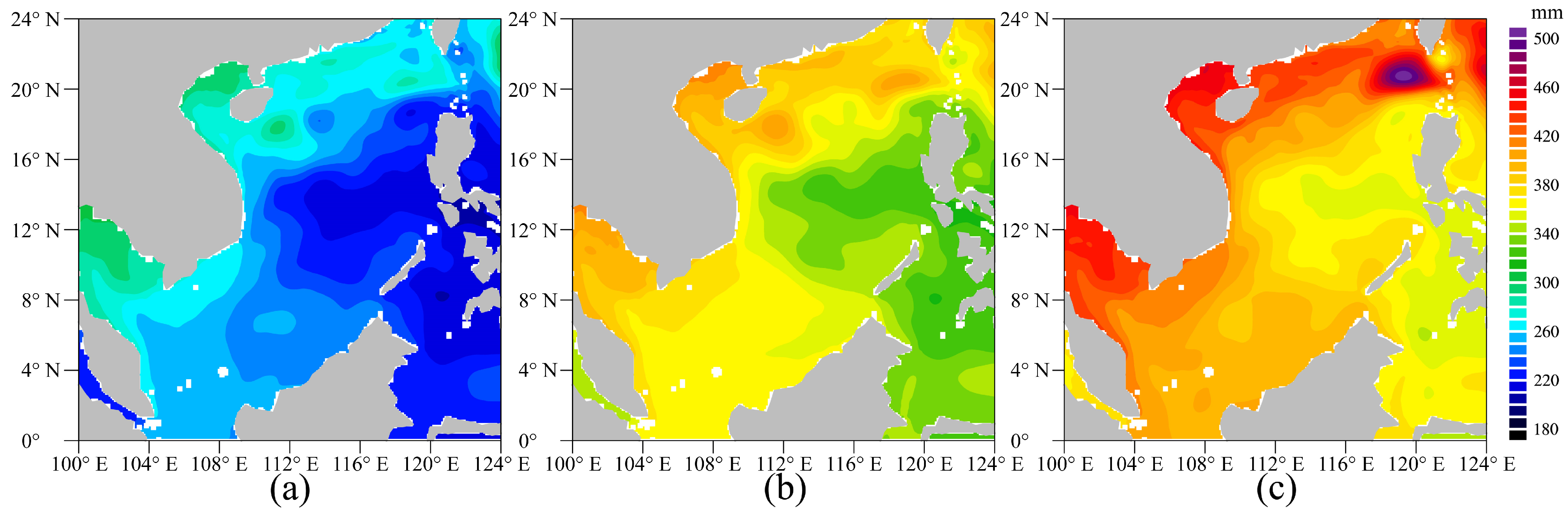
Under three scenarios, the total sea level changes of the SCS in the entire 21st century show a fluctuating upward trend, and the rise magnitude of the sea level height increases with the enhancement of scenarios (Figure 7b). Under the SSP1–2.6 scenario, the mean total sea level in the SCS increased by 298 mm at a rate of 0.40 mm/a by the end of the 21st century; under the SSP2–4.5 scenario, the total sea level increased by 370 mm with a rate of 1.10 mm/a; under the SSP5–8.5 scenario, the total sea level increased by 408 mm at a rate of 1.80 mm/a. It can be seen that the rising trend of the total sea level in the SCS is greater than the rising trend of the local TSSL in the SCS, and because the total sea level is superimposed on changes in the global SSL, the global TSSL contributes significantly to the total sea level in the SCS. From the spatial distribution of the total sea level changes in the SCS at the end of the 21st century under three scenarios, it can be seen that the spatial changes in total sea level are consistent with those in the DSL, but the rise in total sea level is much larger than that in the DSL. Therefore, the spatial changes in the total sea level are dominated by the spatial change DSL, but the magnitude of the total sea level rise is mainly contributed by the global TSSL. Under the SSP1–2.6 scenario, the total sea level in the central and southeastern parts of the SCS rises by 215–250 mm, while the total sea level along the coast rises by 255–295 mm (Figure 9a). Under the SSP2–4.5 scenario, the total sea level in the central and southeastern parts of the SCS rises by 3250–360 mm, while the total sea level along the coast rises by 370–410 mm (Figure 9b). Under the SSP5–8.5 scenario, the total sea level in the central and southeastern parts of the SCS increased by 355–495 mm, while the total sea level along the coast increased by 415–500 mm (Figure 9c). Therefore, the future sea level rise in the SCS will cause more damage to coastal areas.
5. Conclusions
In this study, the simulation capability of 20 models in CMIP6 is tested through the evaluation of sea level height data. According to the correlation coefficient, standard deviation and root mean square deviation of the historical sea level height series of each model and the AVISO sea level height series, seven models with good simulation capability are selected. The average results of these seven models exceed all indicators of all models, which is in good agreement with the observed data. This article uses the average results of the above seven models drive the ROMS, and establishes a high-resolution regional ocean model of the SCS using dynamic downscaling technology. The DSL, SSL, and total sea level changes and their causes in the SCS are analyzed under the SSP1–2.6, SSP2–4.5, and SSP5–8.5 scenarios.
The DSL after dynamic downscaling of ROMS and the average DSL of seven models in CMIP6 have similar large-scale patterns, but their rise amplitude is different, and the spatial change gradient of the DSL after downscaling is more obvious. In the case of downscaling assessment, as more water from the Pacific Basin flows into the SCS through the Luzon Strait, the cyclonic circulation in the upper part of the SCS is strengthened, resulting in negative changes in the DSL in the central and southeast of the SCS. The rise of SSL leads to the redistribution of the seawater mass and the strengthening of the western boundary current, resulting in a greater increase in the coastal DSL. Under three scenarios, the local TSSL of the SCS show a fluctuating upward trend throughout the 21st century, and the rate of rise increases with the enhancement of emission scenarios. By the end of the 21st century, the variation value of the local SSSL in the SCS was much smaller than that of local TSSL. Therefore, the local SSL was dominated by local TSSL. The changes of local TSSL more than half of the sea level rise in SCS, indicating that the sea level changes in the SCS are mainly contributed by local TSSL change. The DSL obtained by downscaling in the SCS is 30–90 mm higher than the sea level rise in the results driven by eight models of CMIP5 calculated by Jin et al. [19]. The local TSSL obtained by downscaling in the SCS is 360–430 mm higher than the average results of CMIP5 calculated by Liu et al. [17]. Therefore, the TSSL and DSL rise after dynamic downscaling under the CMIP6 scenarios (SSPs) are higher than previous research results based on the CMIP5 scenarios. The spatial distribution of total sea level changes is consistent with DSL changes, but the magnitude of total sea level rise is much larger than that of DSL rise. Therefore, the spatial distribution of total sea level is dominated by DSL, but the magnitude of total sea level rise is mainly contributed by TSSL.
The dynamic downscaling results of the SCS reveal more spatial detail and provide more reliable projection of future sea levels in the context of global warming. Sea level rise along the coast of the SCS will occur at different rates under three scenarios, which will increase the risk of extreme water level disasters in the SCS. The research results of this study can be used to formulate reasonable plans for coastal areas in the SCS to cope with coastal retreat, flooding, and storm surge disasters caused by sea level rise, and provide a reference for evaluating the design and construction cycle and service life of flood control infrastructure [41].
Author Contributions
Conceptualization, Q.J. and J.Z. (Jie Zhang); methodology, Q.J., J.Z. (Juncheng Zuo) and J.L.; validation, J.Z. (Jie Zhang) and Q.J.; formal analysis, J.Z. (Jie Zhang). and Q.J.; investigation, J.Z. (Jie Zhang).; resources, Q.J. and H.L.; writing—original draft preparation, J.Z. (Jie Zhang).; writing—review and editing, Q.J., Z.Z., X.L. and Z.W.; visualization, J.Z. (Jie Zhang); funding acquisition, Q.J., J.Z. (Juncheng Zuo), J.L. and H.L. All authors have read and agreed to the published version of the manuscript.
Funding
This research was funded by National Natural Science Foundation of China under granted numbers 42130402 and 42176012, National Key Research and Development Program of China under grant No. 2017YFA0604901 and National Natural Science Foundation of China under granted numbers 41976025, 42006021 and 42076233.
Institutional Review Board Statement
Not applicable.
Informed Consent Statement
Not applicable.
Data Availability Statement
Due to the nature of this study, the participants did not agree to their data being shared publicly; therefore, supporting data are unavailable.
Acknowledgments
The authors would like to thank the editor and the anonymous reviewers for their useful suggestions and comments that helped to improve the paper and the presentation.
Conflicts of Interest
The authors declare no conflict of interest.
References
- Peltier, W.R.; Tushingham, A.M. Global Sea Level Rise and the Greenhouse Effect: Might They Be Connected? Science 1989, 244, 806–810. [Google Scholar] [CrossRef]
- Cazenave, A.; Cozannet, G.L. Sea level rise and its coastal impacts. Earths Future 2013, 2, 15–34. [Google Scholar] [CrossRef]
- IPCC. Climate Change 2013: The Physical Science Basis. Contribution of Working Group I to the Fifth Assessment Report of the Intergovernmental Panel on Climate Change; Stocker, T.F., Qin, D., Plattner, G.-K., Tignor, M., Allen, S.K., Boschung, J., Nauels, A., Xia, Y., Bex, V., Midgley, P.M., Eds.; Cambridge University Press: Cambridge, UK; New York, NY, USA, 2013; pp. 1–1535. [Google Scholar]
- IPCC. Climate Change 2021: The Physical Science Basis. Contribution of Working Group I to the Sixth Assessment Report of the Intergovernmental Panel on Climate Change; Masson-Delmotte, V., Zhai, P., Pirani, A., Connors, S.L., Péan, C., Berger, S., Caud, N., Chen, Y., Goldfarb, L., Gomis, M.I., Eds.; Cambridge University Press: Cambridge, UK; New York, NY, USA, 2021; in press. [Google Scholar]
- Cazenave, A.; Moreira, L. Contemporary sea-level changes from global to local scales: A review. Proc. R. Soc. A 2022, 478, 20220049. [Google Scholar] [CrossRef]
- Gregory, J.M.; Griffies, S.M.; Hughes, C.W.; Hughes, C.W.; Lowe, J.A.; Church, J.A.; Fukimori, I.; Gomez, N.; Kopp, R.E.; Landerer, F.; et al. Concepts and Terminology for Sea Level: Mean, Variability and Change, Both Local and Globa. Surv. Geophys. 2019, 40, 1251–1289. [Google Scholar] [CrossRef]
- Stammer, D.; Cazenave, A.; Ponte, R.M.; Tamisiea, M.E. Causes for Contemporary Regional Sea Level Changes. Annu. Rev. Mar. Sci. 2013, 5, 21–46. [Google Scholar] [CrossRef] [PubMed]
- Church, J.A.; White, N.J.; Konikow, L.F.; Domingues, C.M.; Cogley, J.G.; Rignot, E.; Gregory, J.M.; van den Broeke, M.R.; Monaghan, A.J.; Velicogna, I. Revisiting the Earth’s sea-level and energy budgets from 1961 to 2008. Geophys. Res. Lett. 2011, 38, L18601. [Google Scholar] [CrossRef]
- Yan, M.; Zuo, J.; Fu, S.; Chen, M.; Cao, Y. Advances on sea level variation research in global and China sea. Mar. Environ. Res. 2008, 27, 197–200. [Google Scholar]
- Zhang, J.; Zuo, J.; Li, J.; Chen, M. Sea level viarations in the South China Sea during the 21st century under RCP4.5. Acta. Oceanol. Sin. 2014, 36, 21–29. [Google Scholar] [CrossRef]
- Brown, S.; Nicholls, R.J.; Lowe, J.A.; Hinkel, J. Spatial variations of sea-level rise and impacts: An application of DIVA. Clim. Chang. 2016, 134, 403–416. [Google Scholar] [CrossRef]
- Hallegatte, S.; Green, C.; Nicholls, R.J.; Corfee-Morlot, J. Future flood losses in major coastal cities. Nat. Clim. Change 2013, 3, 802–806. [Google Scholar] [CrossRef]
- Hermans, T.H.J.; Gregory, J.M.; Palmer, M.D.; Ringer, M.A.; Katsman, C.A.; Slangen, A.B.A. Projecting global mean sea-level change using CMIP6 models. Geophys. Res. Lett. 2021, 48, e2020GL092064. [Google Scholar] [CrossRef]
- Yin, J. Century to multi-century sea level rise projections from CMIP5 models. Geophys. Res. Lett. 2012, 39, L17709. [Google Scholar] [CrossRef]
- Zuo, J.; Zuo, C.; Li, J.; Chen, M.X. Advances in research on sea level variations in China from 2006 to 2015. J. Hohai Univ. 2015, 43, 442–449. [Google Scholar] [CrossRef]
- Liu, R.; Liu, X.D.; Liu, H. Projection of the 21st century sea level change in East China Sea and South China Sea based on CMIP5 model results. J. Earth. Environ. 2020, 11, 412–428. [Google Scholar] [CrossRef]
- Chen, C.; Wang, G.; Yan, Y.; Luo, Y. Projected sea level rise on the continental shelves of the China Seas and the dominance of mass contribution. Environ. Res. Lett. 2021, 16, 64040. [Google Scholar] [CrossRef]
- Huang, C.; Qiao, F. Sea level rise projection in the South China Sea from CMIP5 models. Acta Oceanol. Sin. 2015, 34, 31–41. [Google Scholar] [CrossRef]
- Jin, Y.; Zhang, X.; Church, J.A.; Bao, X.W. Projected sea-level changes in the marginal seas near China based on dynamical downscaling. J. Clim. 2021, 34, 7037–7055. [Google Scholar] [CrossRef]
- Griffies, S.M.; Danabasoglu, G.; Durack, P.J.; Adcroft, A.J.; Balaji, V.; Böning, C.W.; Chassignet, E.P.; Curchitser, E.; Deshayes, J.; Drange, H.; et al. OMIP contribution to CMIP6: Experimental and diagnostic protocol for the physical component of the Ocean Model Intercomparison Project. Geosci. Model. Dev. 2016, 9, 3231–3296. [Google Scholar] [CrossRef]
- Jevrejeva, S.; Palanisamy, H.; Jackson, L.P. Global mean thermosteric sea level projections by 2100 in CMIP6 climate models. Environ. Res. Lett. 2020, 16, 14028. [Google Scholar] [CrossRef]
- Fowler, H.J.; Blenkinsop, S.; Tebaldi, C. Linking climate change modelling to impacts studies: Recent advances in downscaling techniques for hydrological modelling. Int. J. Climatol. 2007, 27, 1547–1578. [Google Scholar] [CrossRef]
- Wang, J.; Church, J.A.; Zhang, X.; Chen, X. Reconciling global mean and regional sea level change in projections and observations. Nat. Commun. 2021, 12, 990. [Google Scholar] [CrossRef]
- Grose, M.R.; Narsey, S.; Delage, F.P.; Dowdy, A.J.; Bador, M.; Boschat, G.; Chung, C.; Kajtar, J.B.; Rauniyar, S.; Freund, M.B.; et al. Insights from CMIP6 for Australia’s future climate. Earths Future 2020, 8, e2019EF001469. [Google Scholar] [CrossRef]
- Lyu, K.; Zhang, X.; Church, J.A.; Hu, J. Evaluation of the interdecadal variability of sea surface temperature and sea level in the Pacific in CMIP3 and CMIP5 models. Int. J. Climatol. 2016, 36, 3723–3740. [Google Scholar] [CrossRef]
- Seo, G.H.; Cho, Y.K.; Choi, B.J.; Kim, K.Y.; Kim, B.; and Tak, Y. Climate change projection in the Northwest Pacific marginal seas through dynamic downscaling. J. Geophys. Res. Ocean. 2014, 119, 3497–3516. [Google Scholar] [CrossRef]
- Kim, Y.; Kim, B.; Jeong, K.Y.; Lee, E.; Byun, D.; Cho, Y. Local Sea-Level Rise Caused by Climate Change in the Northwest Pacific Marginal Seas Using Dynamical Downscaling. Front. Mar. Sci. 2021, 8, 620570. [Google Scholar] [CrossRef]
- Frederikse, T.; Landerer, F.; Caron, L.; Adhikari, S.; Parkes, D.; Humphrey, V.W.; Dangendorf, S.; Hogarth, P.; Zanna, L.; Cheng, L.; et al. The causes of sea-level rise since 1900. Nature 2020, 584, 393–397. [Google Scholar] [CrossRef] [PubMed]
- Milne, G.A.; Gehrels, W.R.; Hughes, C.; Tamisiea, M.E. Identifying the causes of sea-level change. Nat. Geosci. 2009, 2, 471–478. [Google Scholar] [CrossRef]
- Tabata, S.; Thomas, B.; Ramsden, D. Annual and Interannual Variability of Steric Sea Level along Line P in the Northeast Pacific Ocean. J. Phys. Oceanogr. 1986, 16, 1378–1398. [Google Scholar] [CrossRef]
- Chen, C.; Zuo, J.; Chen, M.; Gao, Z.; SHUM, C. Sea level change under IPCC-A2 scenario in Bohai, Yellow, and East China Seas. Water Sci. Eng. 2014, 7, 446–456. [Google Scholar] [CrossRef]
- ICES; SCOR; IAPSO. Tenth Report of the Join Panel on Oceanographic Tables and Standards (The Practical Salinity Scale 1978 and the International Equation of State of Seawater 1980); UNESCO Technical Papers in Marine Science No. 36: Paris, French, 1981; pp. 1–25. [Google Scholar]
- Antonov, J.I.; Levitus, S.; Boyer, T.P. Thermosteric sea level rise, 1955–2003. Geophys. Res. Lett. 2005, 32, L12602. [Google Scholar] [CrossRef]
- Greatbatch, R.J. A note on the representation of steric sea level in models that conserve volume rather than mass. J. Geophys. Res. 1994, 99, 12767–12771. [Google Scholar] [CrossRef]
- Mellor, G.L.; Ezer, T. Sea level variations induced by heating and cooling: An evaluation of the Boussinesq approximation in ocean models. J. Geophys. Res. Ocean. 1995, 100, 20565. [Google Scholar] [CrossRef]
- Tedeschi, R.G.; Collins, M. The influence of ENSO on South American precipitation: Simulation and projection in CMIP5 models. Int. J. Climatol. 2017, 37, 3319–3339. [Google Scholar] [CrossRef]
- Xu, T.; Cao, Y. Numerical Simulation Study on the Seasonal Variations of Ocean Circulations in the South China Sea. Coast. Eng. 2017, 36, 62–71. [Google Scholar] [CrossRef]
- Maximenko, N.; Niiler, P.; Centurioni, L.; Rio, M.; Melnichenko, O.; Chambers, D.; Zlotnicki, V.; Galperin, B. Mean Dynamic Topography of the Ocean Derived from Satellite and Drifting Buoy Data Using Three Different Techniques. J. Atmos. Ocean. Technol. 2009, 26, 1910–1919. [Google Scholar] [CrossRef]
- Yin, J.; Griffies, S.M.; Stouffer, R.J. Spatial Variability of Sea Level Rise in Twenty-First Century Projections. J. Clim. 2010, 23, 4585–4607. [Google Scholar] [CrossRef]
- Wang, G.; Xie, S.; Huang, R.X.; Chen, C. Robust Warming Pattern of Global Subtropical Oceans and Its Mechanism. J. Clim. 2015, 28, 8574–8584. [Google Scholar] [CrossRef]
- Vousdoukas, M.I.; Mentaschi, L.; Voukouvalas, E.; Verlaan, M.; Jevrejeva, S.; Jackson, L.P.; Feyen, L. Global probabilistic projections of extreme sea levels show intensification of coastal flood hazard. Nat. Commun. 2018, 9, 2360. [Google Scholar] [CrossRef]
Figure 1.
Climatological mean (1993–2014) SSH in offshore China from 20 CMIP6 models (a–t) and observed data (AVISO) (u).
Figure 1.
Climatological mean (1993–2014) SSH in offshore China from 20 CMIP6 models (a–t) and observed data (AVISO) (u).
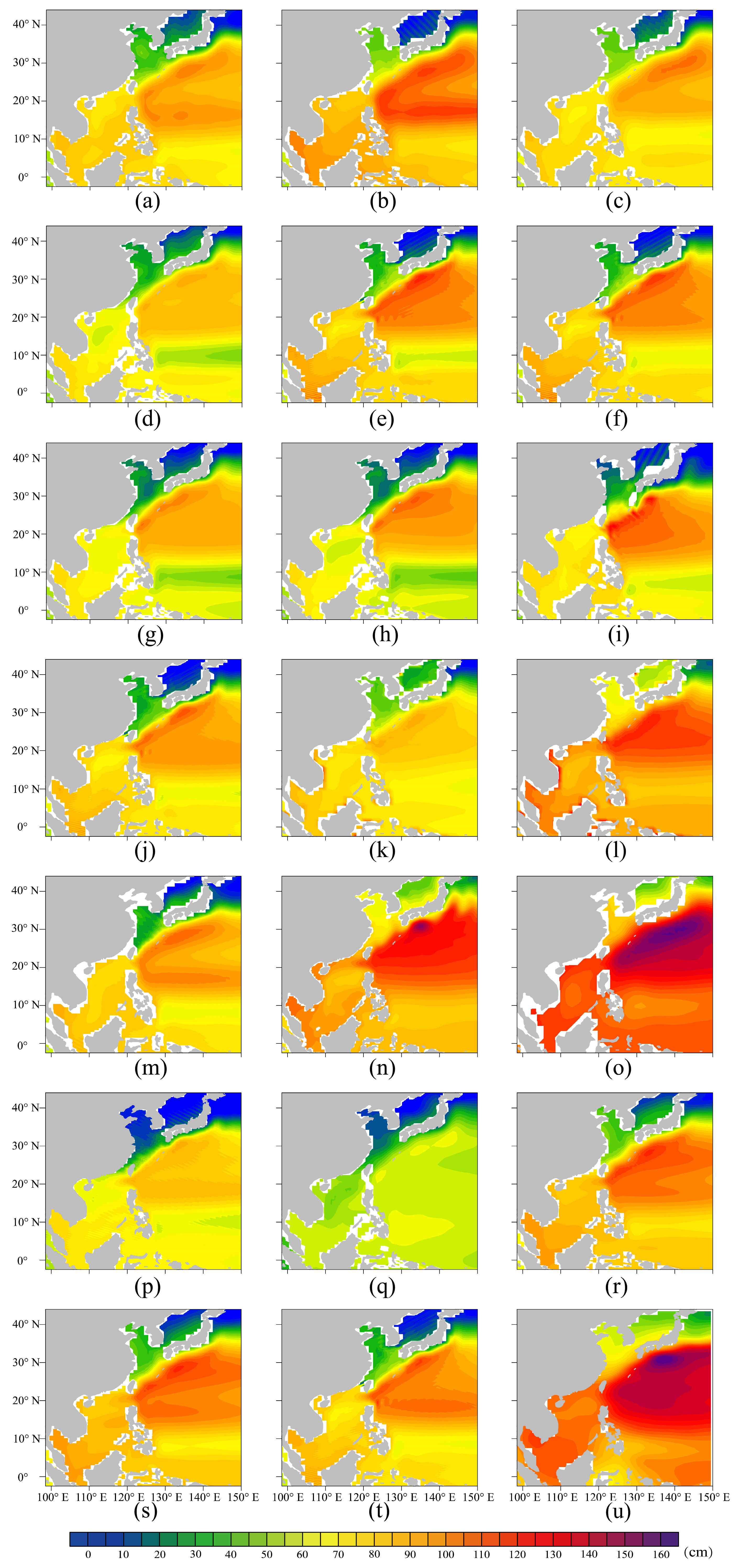
Figure 2.
Distributions of Taylor diagram for displaying normalized pattern statistics of SSH over offshore China from 20 CMIP6 models and observation reference (AVIOS). The letters (a–t) are consistent with the numbering of each mode in Table 1. The red dots represent the 7 selected modes with better simulation results, while the black dots represent the 10 selected modes with better simulation results. The “v” represents the average result of these 10 models, and “w” represents the average result of all 20 models; The REF point represents the observed SSH, where the distance from the position of the point to the origin represents the ratio of the standard deviation between the simulation and the observation results, the bearing angle corresponding to the point represents the correlation coefficient between the simulation and the observation field. The distance of the letter to REF indicates the center after normalization of the standard deviation of the observing field root mean square error.
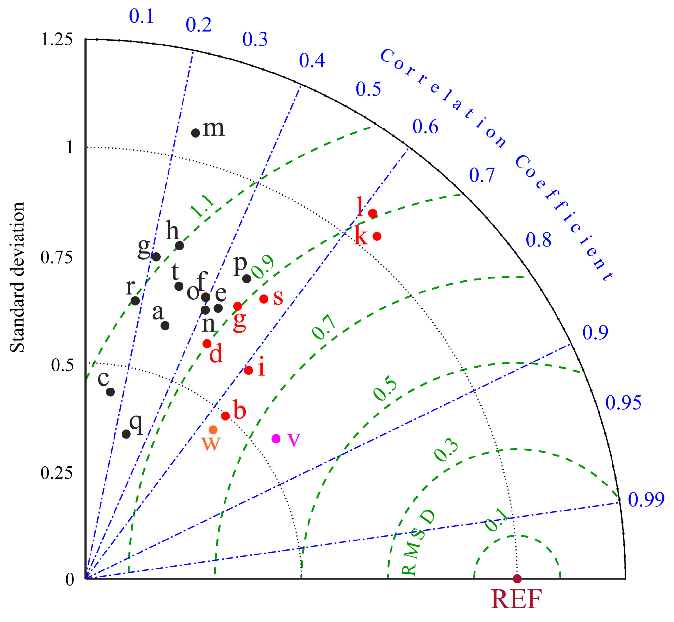
Figure 3.
Simulated summer climate state current field (a), OSCAR summer climate state observation current field (b), simulated winter climate state current field (c), and OSCAR winter climate state observation current field (d) from 1993 to 2014.
Figure 3.
Simulated summer climate state current field (a), OSCAR summer climate state observation current field (b), simulated winter climate state current field (c), and OSCAR winter climate state observation current field (d) from 1993 to 2014.
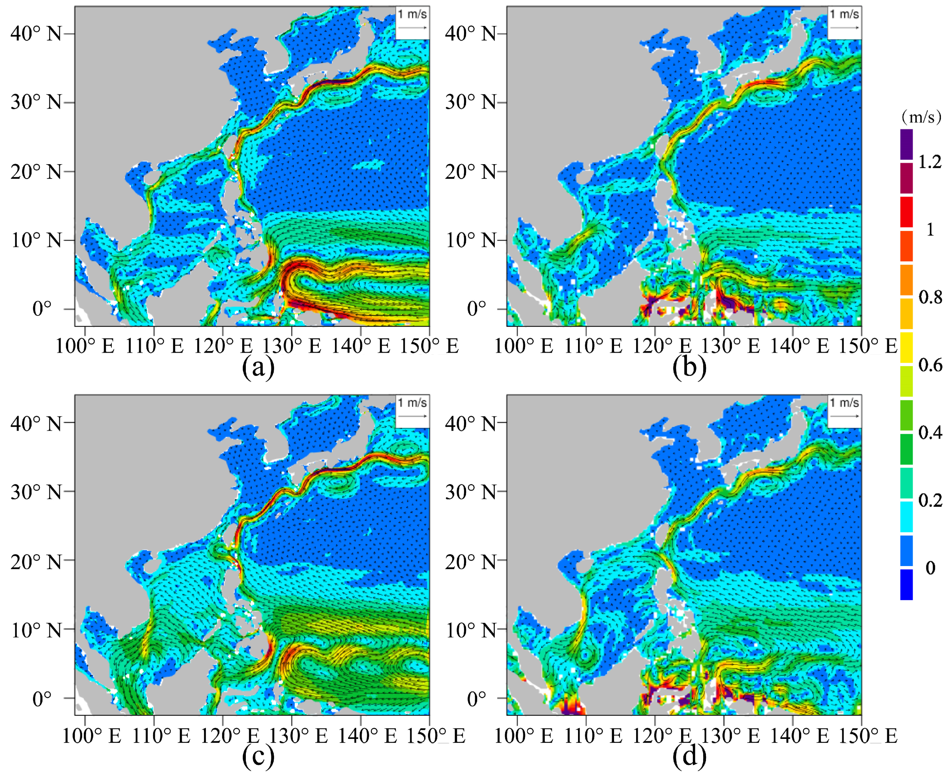
Figure 4.
Simulated climate state SST (a), climate state SST of WOA (b), simulated climate state SSS (c), and climate state SSS of WOA (d) from 1995 to 2004. Simulated climate state DSL (e) and the average DSL of 7 models in CMIP6 (f) from 1980 to 2014.
Figure 4.
Simulated climate state SST (a), climate state SST of WOA (b), simulated climate state SSS (c), and climate state SSS of WOA (d) from 1995 to 2004. Simulated climate state DSL (e) and the average DSL of 7 models in CMIP6 (f) from 1980 to 2014.

Figure 5.
The spatial distribution of DSL changes for ROMS under SSP1–2.6 scenario (a), SSP2–4.5 scenario (b), SSP5–8.5 scenario (c) and the average DSL of 7 models in CMIP6 under the SSP1–2.6 scenario (d), SSP2–4.5 scenario (e), and SSP5–8.5 scenario (f) at the end of 21st century.
Figure 5.
The spatial distribution of DSL changes for ROMS under SSP1–2.6 scenario (a), SSP2–4.5 scenario (b), SSP5–8.5 scenario (c) and the average DSL of 7 models in CMIP6 under the SSP1–2.6 scenario (d), SSP2–4.5 scenario (e), and SSP5–8.5 scenario (f) at the end of 21st century.
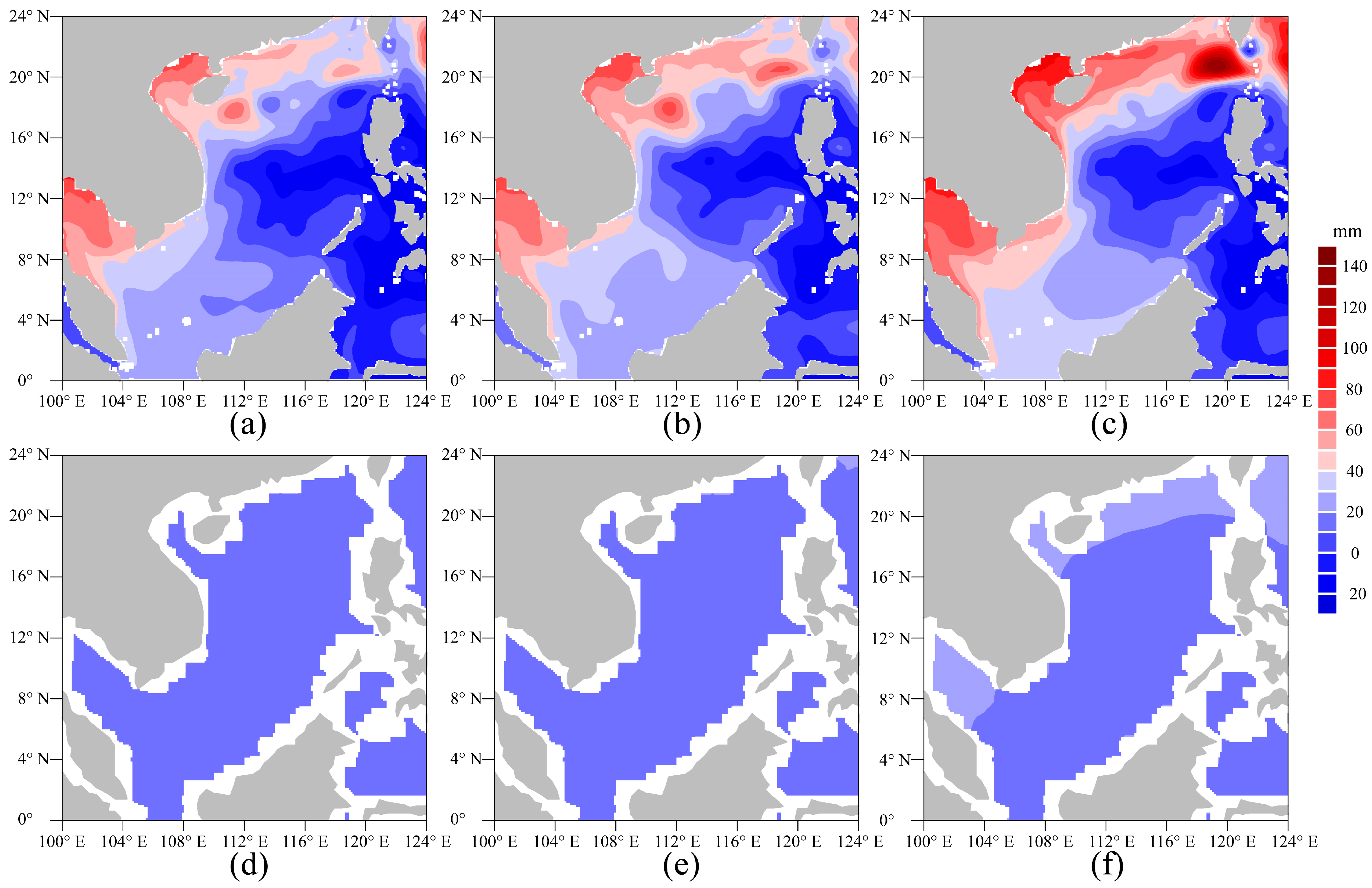
Figure 6.
The upper 55 m volume transport of the east boundary from the Historical experiment and the future experiment (SSP1–2.6, SSP2–4.5 SSP5–8.5) (a), and their difference (future period minus historical period) (b).
Figure 6.
The upper 55 m volume transport of the east boundary from the Historical experiment and the future experiment (SSP1–2.6, SSP2–4.5 SSP5–8.5) (a), and their difference (future period minus historical period) (b).
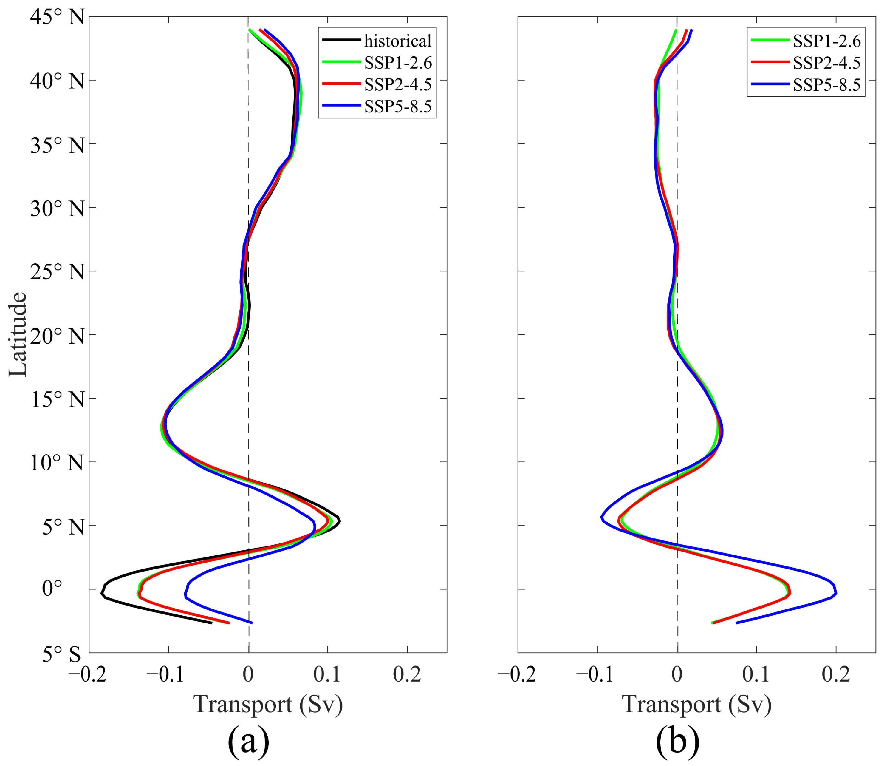
Figure 7.
Time series changes of local TSSL (a) and total sea level (b) in the 21st century under three scenarios.
Figure 7.
Time series changes of local TSSL (a) and total sea level (b) in the 21st century under three scenarios.
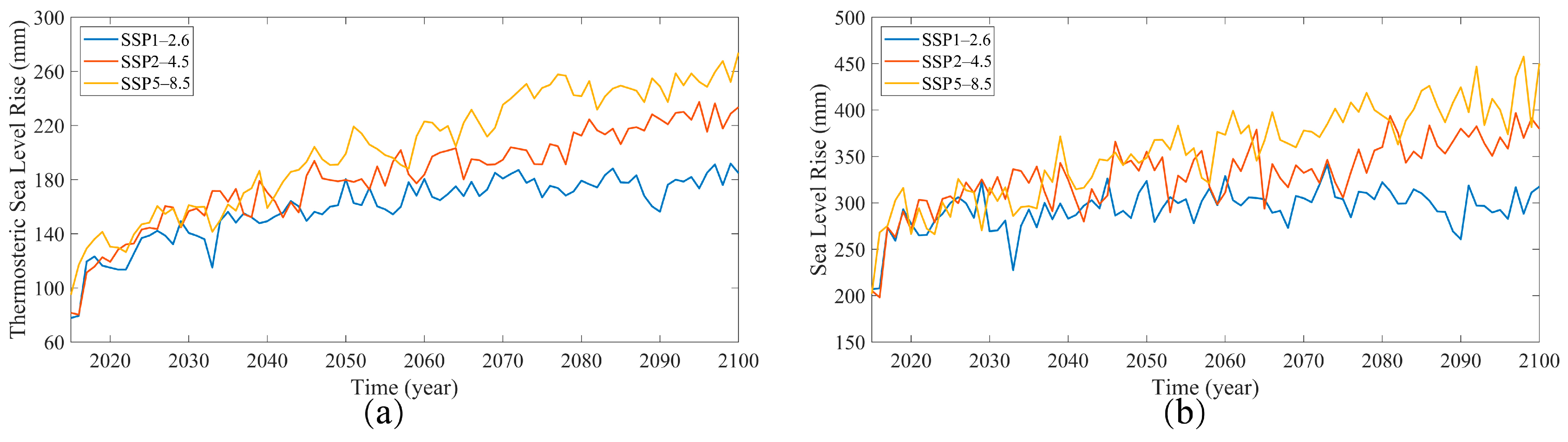
Figure 8.
The spatial distribution of TSSL changes for ROMS under the SSP1-2.6 scenario (a), SSP2-4.5 scenario (b) and SSP5-8.5 scenario (c) at the end of 21st century.
Figure 8.
The spatial distribution of TSSL changes for ROMS under the SSP1-2.6 scenario (a), SSP2-4.5 scenario (b) and SSP5-8.5 scenario (c) at the end of 21st century.
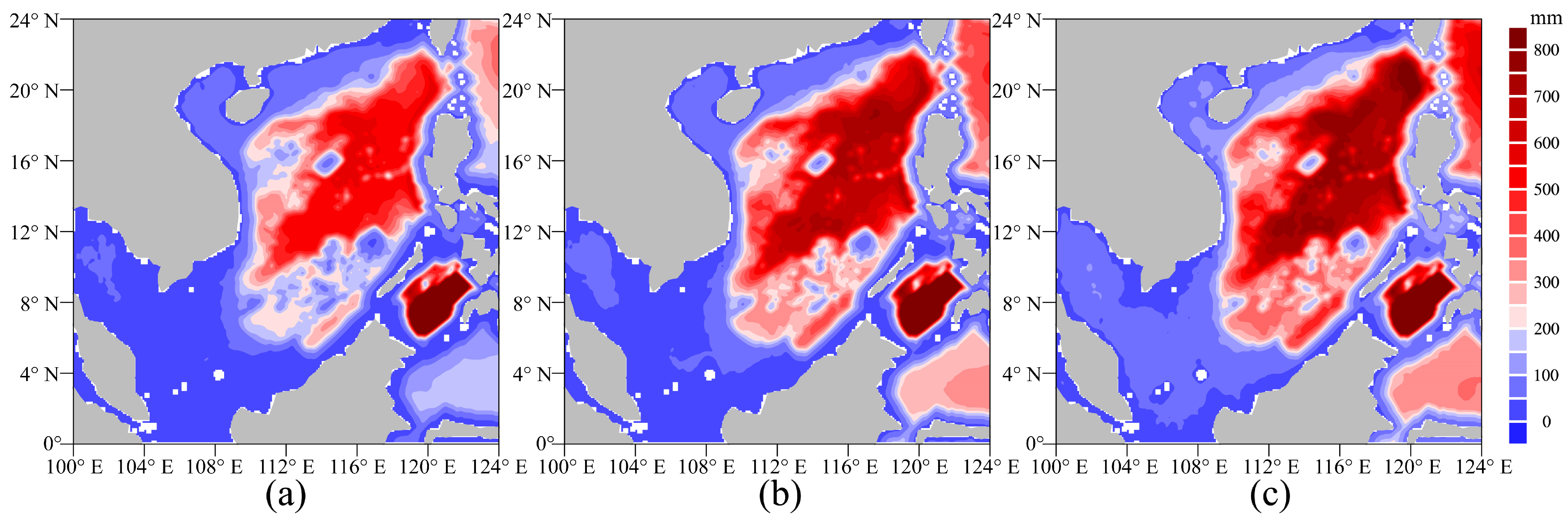
Figure 9.
The spatial distribution of all sea level changes for ROMS under the SSP1-2.6 scenario (a), SSP2-4.5 scenario (b) and SSP5-8.5 scenario (c) at the end of 21st century.
Figure 9.
The spatial distribution of all sea level changes for ROMS under the SSP1-2.6 scenario (a), SSP2-4.5 scenario (b) and SSP5-8.5 scenario (c) at the end of 21st century.

Table 1.
The CMIP6 model used in this article and its affiliated institutions, atmospheric and oceanic horizontal resolutions (unit: km).
Table 1.
The CMIP6 model used in this article and its affiliated institutions, atmospheric and oceanic horizontal resolutions (unit: km).
| ID | Source | Institution | Atmosphere | Ocean |
|---|---|---|---|---|
| a | ACCESS-CM2 | ACCESS | 250 | 250 |
| b * | BCC-CSM2-MR | BCC | 100 | 100 |
| c | CAMS-CSM1-0 | CAMS | 100 | 100 |
| d * | CanESM5 | CCCma | 500 | 100 |
| e | CESM2 | NCAR | 100 | 100 |
| f | CESM2-WACCM | NCAR | 100 | 100 |
| g * | CMCC-CM2-SR5 | CMCC | 100 | 100 |
| h | CMCC-ESM2 | CMCC | 100 | 100 |
| i * | FGOALS-g3 | CAS | 250 | 100 |
| j | FIO-ESM-2-0 | FIO-QLNM | 100 | 100 |
| k * | GISS-E2-1-G | NASA-GISS | 250 | 250 |
| l * | GISS-E2-2-G | NASA-GISS | 250 | 250 |
| m | MIROC6 | MIROC | 250 | 100 |
| n | MPI-ESM1-2-HR | MPI-M | 100 | 50 |
| o | MPI-ESM1-2-LR | MPI-M | 250 | 250 |
| p | MRI-ESM2-0 | MRI | 100 | 100 |
| q | NESM3 | NUIST | 250 | 100 |
| r | NorESM2-LM | NCC | 250 | 100 |
| s * | NorESM1-MM | NCC | 100 | 100 |
| t | TaiESM1 | AS-RCEC | 100 | 100 |
| v | The average results of 7 models | |||
| w | The average results of 20 models | |||
* Represents selected models.
Disclaimer/Publisher’s Note: The statements, opinions and data contained in all publications are solely those of the individual author(s) and contributor(s) and not of MDPI and/or the editor(s). MDPI and/or the editor(s) disclaim responsibility for any injury to people or property resulting from any ideas, methods, instructions or products referred to in the content. |
© 2023 by the authors. Licensee MDPI, Basel, Switzerland. This article is an open access article distributed under the terms and conditions of the Creative Commons Attribution (CC BY) license (https://creativecommons.org/licenses/by/4.0/).
Share and Cite
MDPI and ACS Style
Zhang, J.; Ji, Q.; Zuo, J.; Li, J.; Zhang, Z.; Li, H.; Liu, X.; Wang, Z. Projection of Sea Level Change in the South China Sea Based on Dynamical Downscaling. Atmosphere 2023, 14, 1343. https://doi.org/10.3390/atmos14091343
AMA Style
Zhang J, Ji Q, Zuo J, Li J, Zhang Z, Li H, Liu X, Wang Z. Projection of Sea Level Change in the South China Sea Based on Dynamical Downscaling. Atmosphere. 2023; 14(9):1343. https://doi.org/10.3390/atmos14091343
Chicago/Turabian StyleZhang, Jie, Qiyan Ji, Juncheng Zuo, Juan Li, Zheen Zhang, Huan Li, Xing Liu, and Zhizu Wang. 2023. "Projection of Sea Level Change in the South China Sea Based on Dynamical Downscaling" Atmosphere 14, no. 9: 1343. https://doi.org/10.3390/atmos14091343
Note that from the first issue of 2016, this journal uses article numbers instead of page numbers. See further details here.