
Computational Domain Size Effects on Large-Eddy Simulations of Precipitating Shallow Cumulus Convection

1
Department of Civil and Environmental Engineering, University of Connecticut, Storrs, CT 06269, USA
2
Department of Mechanical Engineering, University of Connecticut, Storrs, CT 06269, USA
3
Jet Propulsion Laboratory, California Institute of Technology, Pasadena, CA 91125, USA
*
Author to whom correspondence should be addressed.
Atmosphere 2023, 14(7), 1186; https://doi.org/10.3390/atmos14071186
Submission received: 7 June 2023
/
Revised: 30 June 2023
/
Accepted: 4 July 2023
/
Published: 22 July 2023
(This article belongs to the Section Atmospheric Techniques, Instruments, and Modeling)
Abstract
:Idealized large-eddy simulations of shallow convection often utilize horizontally periodic computational domains. The development of precipitation in shallow cumulus convection changes the spatial structure of convection and creates large-scale organization. However, the limited periodic domain constrains the horizontal variability of the atmospheric boundary layer. Small computational domains cannot capture the mesoscale boundary layer organization and artificially constrain the horizontal convection structure. The effects of the horizontal domain size on large-eddy simulations of shallow precipitating cumulus convection are investigated using four computational domains, ranging from to and fine grid resolution (40 m). The horizontal variability of the boundary layer is captured in computational domains of . Small LES domains (≤40 km) cannot reproduce the mesoscale flow features, which are about long, but the boundary layer mean profiles are similar to those of the larger domains. Turbulent fluxes, temperature and moisture variances, and horizontal length scales are converged with respect to domain size for domains equal to or larger than . Vertical velocity flow statistics, such as variance and spectra, are essentially identical in all domains and show minor dependence on domain size. Characteristic horizontal length scales (i.e., those relating to the mesoscale organization) of horizontal wind components, temperature and moisture reach an equilibrium after about hour 30.
1. Introduction
Clouds forming in the atmospheric boundary layer play a crucial role in the Earth’s energy balance as they influence radiative transfer, surface energy fluxes and the hydrological cycle [1,2,3]. Shallow clouds, in particular, have been identified as one of the main sources of uncertainty in climate projections [1]. Precipitation alters the boundary layer spatial structure, leading to large-scale organization [4]. Accurate simulations of shallow cumulus convection are thus essential for improving climate models and reducing uncertainties in future projections.
Large-eddy simulation (LES) is a major research tool in atmospheric boundary layer studies. LES is a “turbulence resolving” model that yields a physically consistent description of the spatial variability over a large range of scales [5,6]. For example, in investigations of processes in shallow cumulus convection [7,8,9,10,11,12]. The domain size in LES can significantly impact the simulated cloud fields and boundary layer structure [13,14]. Particularly in idealized process-level LES investigations where periodic boundary conditions in the horizontal directions are used. A growing body of literature has explored the influence of domain size on LES of shallow cumulus convection [6,13,14,15,16,17,18]. For instance, refs. [12,14] demonstrated that increasing domain size could lead to the formation of larger convective structures.
Several studies focused on the effects of precipitation on shallow cumulus convection [19,20]. Precipitation can alter the spatial organization of clouds, leading to the formation of large persistent structures [1]. Even in non-precipitating cumulus convection, variance accumulation at the largest scales and generation of large horizontal structures is observed [21]. The interplay between domain size and precipitation remains relatively unexplored. Lamaakel and Matheou [12] showed that larger domains were required to accurately capture the cloud organization in precipitating shallow convection. Whereas [12] studied the development of shallow convective organization in relatively large LES computational domains, up to , presently we focus on the boundary layer steady state, which occurs after mesoscale organization has been formed.
This study examines the effects of computational domain size on the equilibrium state of a typical case of trade-wind precipitating shallow cumulus convection. The present investigation is the extension of previous work [12] to steady state boundary layers. One important open question from that study [12] is whether the horizontal length scales will continue to grow or reach a steady state. Previous LES investigations suggested that feedbacks can influence mesoscale variability of domain-mean properties and “very large computations are required to obtain meaningful cloud statistics” [15]. To help achieve this goal, an additional run to those of [12] with an unprecedented combination of domain size ( in the horizontal directions) and fine grid resolution () is carried out.
Section 2 briefly describes the LES model and the setup of the simulations. Results are discussed in Section 3. The LES output for different domain sizes is compared with respect to domain-averaged statistics versus time, vertical profiles at the end of the run, spectra and horizontal length scales. First, the evolution of cloud organization is presented, followed by physical-space turbulent flow statistics. In the second part of the results, spectra and length scales are discussed. Finally, conclusions are summarized in Section 4.
2. Methods
The LES model of [22] is used to simulate shallow convection in a trade-wind atmospheric boundary layer. The LES model numerically integrates the anelastic approximation of the equations of motion on an f-plane. Warm rain processes are parameterized with the two-moment bulk warm-rain parameterization of Seifert and Beheng [23] and turbulent transport is parameterized with the buoyancy-adjusted stretched-vortex subgrid scale (SGS) model [24]. The buoyancy-adjusted stretched-vortex model is a state of the art structural turbulence closure that accounts for both the anisotropy of the SGS flow and density-stratification effects. Momentum, liquid water potential temperature and total water mixing ratio advection terms are approximated with the fourth-order centered fully conservative scheme of [25]. Microphysical-variable advection terms are discretized with a monotone flux-limited scheme to ensure water-mass conservation. The third-order Runge–Kutta method of [26] is used for time integration. To limit gravity wave reflections, a Rayleigh damping layer is used at the top of the domain.
The idealized case corresponding to the Rain In shallow Cumulus over the Ocean (RICO) observational campaign is simulated [27,28]. The initial soundings have a typical trade-wind cumulus-topped boundary layer structure. Large-scale forcings include a constant in time geostrophic wind, subsidence, advective tendencies and clear air radiative cooling. Surface fluxes are dynamically computed using a constant sea surface temperature (SST) bulk parameterization following [28].
Simulations with progressively larger domain sizes are carried out. All domains are square in the horizontal directions, i.e., equal domain size lengths . The boundary conditions are doubly periodic in the horizontal. The x and y coordinates are along the zonal and meridional directions, respectively. The smallest domain size has , which is twice as large in each direction compared to the LES domains used in the model intercomparison [28]. The domain horizontal length doubles in each direction as the domain sizes increase in the present runs: , 81.92, 163.84 and . The setup of the runs is shown in Table 1. The simulations are labeled A to D in the order of increasing computational domain size. A uniform and isotropic grid spacing is used. The simulations are performed in a horizontally translating frame of reference with approximately the domain-mean wind [11]. The simulations are run for to reach a statistically stationary state. A statistically steady state is expected after [8,10]. The case setup does not include any diurnal cycle effects and the forcings are constant through the duration of the run.
The two largest runs, C and D, are fairly large computations. The largest simulation consists of 8.3 billion grid cells. Large-scale organization develops after , see [7,8,10,12,28], whereas during the first part of the simulations () homogeneous scattered cumulus develop and progressively deepen. As discussed in [12], smaller domains sufficiently capture the organization and flow statistics for . Therefore, run D is initialized based on run C output at , to save computing time. The output of run C is repeated in a pattern to span the twice larger in each direction domain D. Random temperature and moisture perturbations are added in the lowest to help randomize the periodic pattern. After run D becomes de-correlated from run C.
Model validation and sensitivity to model parameters are discussed in [22]. In addition, the present simulations yield cloud patterns, including their horizontal dimensions, similar to the observations in [27,29,30] and other model results [19,28,31]. At the present grid resolution , the LES generates grid-independent results [22]. Further validation and assessment of the LES model for a diverse set of meteorological conditions is discussed in [7,32,33,34,35,36,37].
3. Results
3.1. Convection Organization
The organization of convection is visualized in Figure 1 and Figure 2 by plotting contours of cloud-liquid water path (LWP) and rain water path (RWP) fields at . All four LES domains are shown in each figure directly displaying the differences in area coverage of each domain. The characteristic structure of shallow precipitating convection with cold pools, cloud arcs and occasional stratiform cloud anvils, similar to observations and previous modeling [8,10] is clear in the largest domains. A comparison between the LWP and RWP fields shows the locations of stratiform cloud anvils, which mostly register in the LWP field but not in RWP, because precipitation primarily develops in convective clouds. Most rain develops in the long cumulus clusters that form the cloud arcs at the leading boundary of the cold pools.
Structures longer than form in the boundary layer. The spacing between the cloud arcs is similar in the two largest domains C and D. Smaller domains, particularly domain A, are very small compared to the cloud arcs and cold pool structures of runs C and D. Smaller domains cannot realistically represent the size and spacing of cloud arcs and cold pool structures.
3.2. Domain-Averaged Turbulent-Flow Statistics
Figure 3 shows boundary layer statistics averaged over the computational domain volume. Panels correspond to the time evolution of the vertical integral of turbulent kinetic energy, , cloud-liquid (LWP, suspended condensate) and rain water (RWP) paths, cloud statistics (cloud top , base and cloud fraction ), inversion height and surface precipitation rate. The angle brackets denote the instantaneous horizontal average. The inversion height is defined as the height of the maximum potential temperature, , gradient. Cloud base and cloud top are defined as the minimum and maximum heights with a horizontal-mean cloud-liquid water mixing ratio . Lines for run D () start at , an hour after initialization, to remove the initial impulse caused by adding random perturbations when domain D is initialized. Traces between runs C and D show visible differences by hour 25 and larger differences after hour 30. Data for simulations A–C for are the same as those of [12].
Runs C and D show good agreement with respect to domain-averaged statistics. The differences in cloud-top height between C and D are expected, because tracks the domain-maximum of the cloud top. As the domain area increases, the instances of locally higher cloud tops are more likely. As discussed in [12], the area fraction of cloud above the inversion is very small. Thus, high values are not representative of the entire area or the depth of the turbulent layer. See also TKE and profiles in the next section.
3.3. Vertical Profiles
Figure 4 shows profiles at . Profiles are instantaneous horizontal averages without any time averaging. The total water vertical flux is additionally time-averaged in a ten-minute interval to create smoother curves. Turbulent fluxes include both the resolved-scale and subgrid-scale contributions. The time-variability of the profiles is small because all computational domains are relatively large and the horizontal averages include most of the horizontal variability of the boundary layer. The variation with respect to time of the vertical profiles is discussed in Appendix A.
Only the horizontal component of TKE exhibits large differences with respect to domain size. The differences in the TKE profile are caused by the horizontal component . The profiles of Figure 4e,f are essentially identical. Note that the x-axis scale of Figure 4g, the vertical component of TKE, is different than Figure 4e,f. Further, most of the differences in the horizontal component between runs A and B are because of the component (not shown in Figure 4).
With the exception of the moisture flux and , the smallest domain, run A, has the largest differences with respect to the other runs in Figure 4. The two largest domains, runs C and D, are in good agreement for u, , and TKE. Most of the differences between all runs are observed near the inversion layer, . As discussed in the previous section, even though clouds occasionally rise up to , TKE, and the moisture flux are small above the inversion, indicating that very deep clouds have very small area fractions. This is in agreement with previous run C results [12] before the boundary layer reached steady state.
The profiles of wind, and are essentially identical for all domains. Relatively small differences are observed near the inversion layer () between the smallest domain (run A, ) and the rest of the simulations. Larger differences are observed in second-order flow statistics, covariances and TKE. In addition, TKE (Figure 4e) and temperature variance (Figure 5b) are in good agreement only in the two largest-domain runs, C and D. Interestingly, the cloud liquid at steady state (Figure 4d) does not exhibit large differences but temperature and moisture variance (Figure 5) profiles show larger differences, particularly between runs A–B and runs C–D.
3.4. Inversion Strength
The small differences in the mean and profiles near the inversion layer (Figure 4) and larger differences with respect to their variance (Figure 5) motivate the study of the inversion characteristics. Figure 6a shows the inversion strength, defined as the maximum vertical gradient of the mean potential temperature as a function of time. After large-scale organization develops, , the inversion strength evolution significantly differs between run A and the rest of the simulations. The smallest domain run sustains a stronger inversion strength. The inversion strength is a characteristic of the simulated temperature profile, which can be useful in understanding the dynamics of cloud development. For example, a strong inversion layer can limit the upward growth of clouds and restrict their vertical extent, while a weaker inversion layer may allow for more vigorous or deeper cloud development.
Figure 6b shows another diagnostic to help understand the dynamics of the inversion. At the largest computational domain (run D) is partitioned into subdomains in the horizontal. Each of the subdomains has the same horizontal area as domain A. In each of the run D subdomains we compute the inversion strength and the inversion height. These pairs are plotted in Figure 6b as open circles and quantify the inversion strength at the “local” level, whereas the lines of Figure 6a correspond to the entire-domain average of . The domain average is plotted in Figure 6b as a filled circle, which is the same value as the run D line at in Figure 6a. Figure 6b shows that there is large within-domain variability of the inversion strength and height. Values of inversion strength in the D-run subdomains are similar to the inversion strength value of run A. The distribution of values in the y-axis of Figure 6b quantifies the undulations of the inversion in run D, which span about half a km within the area of the simulation. Because of the feedback between the rising cumulus-topped updrafts and the evolution of the trade-wind inversion, a causal relationship between inversion undulations and boundary layer depth cannot be inferred from Figure 6b.
3.5. Spectra and Length Scales
Lamaakel and Matheou [12] studied the growth rate of the horizontal organization in the RICO case. The growth of characteristic horizontal length scales was quantified during the transition from scattered cumulus to the mesoscale-organized cloud clusters shown in Figure 1. Between the horizontal characteristic length scales of u, v, and grow at a rate of 3–, which is in agreement with the growth rate of the developing cold pools. As discussed in [12], the multiple cold pools developing in domain C interact resulting in a boundary layer composed of both scattered cumulus and cloud arcs (Figure 1 and Figure 2). Lamaakel and Matheou [12] studied the first generation of cold pools developing in a fairly homogeneous scattered cumulus field. Presently, we focus on the boundary layer steady state where cold pools are present in various stages of their life cycle and they are interacting. The main question is if the characteristic length scales reach an equilibrium value.
The horizontal characteristic length scales are defined based on the one-dimensional spectra along the longitudinal direction. Similar results are obtained when considering the transverse direction [12]. For u, w, and the x-direction (zonal) is used. For v the meridional direction is used. The one-dimensional premultiplied spectra are shown in Figure 7. The spectra are normalized by the corresponding variance, e.g., for u, the pre-multiplied spectrum is , where is the one-dimensional spectral function, which is computed by performing a two-dimensional discrete Fourier transform on a horizontal plane and then averaging along the wavenumbers. All spectra are computed in the subcloud layer () where the flow is fully turbulent, i.e., three-dimensional turbulence spans the entire layer. In Figure 7 the x-axis is converted from wavenumber to length scale, , to assist the physical interpretation.
The local maxima of the premultiplied spectra are used to identify energy-containing structures. The length scales correspond to narrow wavenumber bands where spectral energy is higher than the neighboring wavenumbers. In the spectra of Figure 7 we are interested in the change of the location of the maxima as well as the shape of the overall curves. Following [12] the spectra are smoothed by a Gaussian filter.
As observed in [12], the vertical velocity spectra do not depend on the domain size and the premultiplied spectrum always has a single peak. The present data extend the observation of [12] regarding the vertical velocity premultiplied spectra to all stages of the boundary layer evolution, from organization development to steady state. Moreover, the characteristic w-velocity scale is small, about , and it is not influenced by the size of the computational domains presently used.
In general, the spectra of runs C and D are in good agreement compared to those of A and B runs. The spectra of runs A and B (except w-velocity) contain more energy at the smaller scales (). Considering that the larger domains result in a more realistic representation of the boundary layer, the smaller domain sizes cause an artificial accumulation of fluctuations at small scales. Further, in some cases (e.g., and , at ) the maxima for runs C and D are at scales larger than the A and B domains.
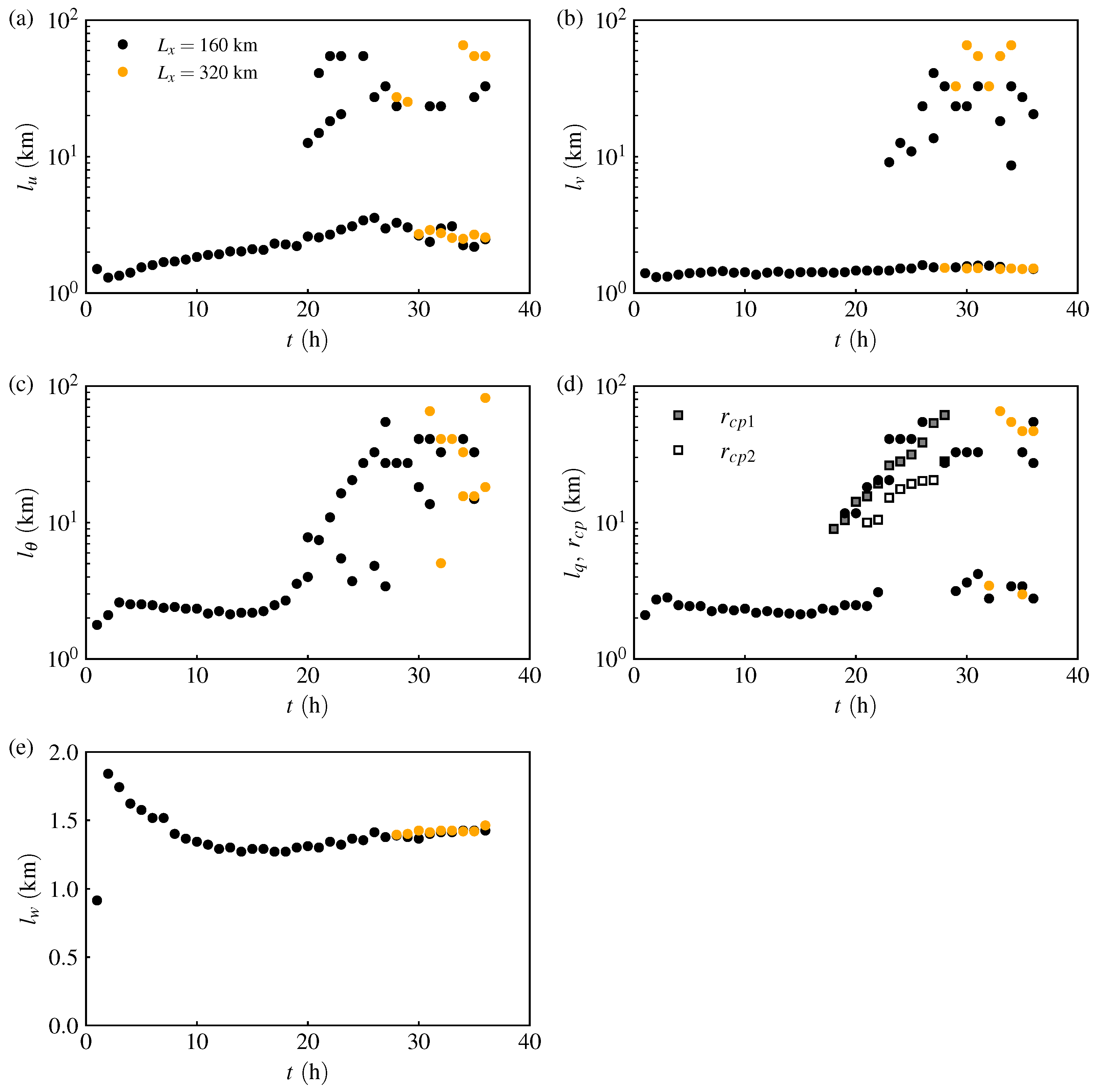
Figure 8 shows the time evolution of characteristic length scales , , , and , where the subscript corresponds to the variable (i.e., corresponds to length scales and to ). Only length scales computed from the output of runs C and D are shown in Figure 8 because their spectra are not sensitive to the domain size. At a given time, i.e., x-coordinate in the plot, multiple symbols for are plotted when the premultiplied spectra have multiple peaks. In Figure 8d, the radii of the first two cold pools and are also shown using the data of [12]. The growth rates of and agree well with . Note that in Figure 8 the y axis of the , , and plots is shown in logarithmic scale to better show the large variability during the evolution of the length scales. Figure 8e corresponds to the vertical velocity length scale. A single length scale is always observed, which grows slowly with time, thus a linear y-axis is used.
Some spectra have sharp peaks between wavenumbers 2 and 4, e.g., Figure 7a,c,h. These peaks do not vary in time and were not included in the data plotted in Figure 8. These peaks are likely artifacts of the periodic domain and do not correspond to physical length scales. Data for domain D are shown after hour 24 to allow sufficient time for run D to de-correlate from the initial condition that was based on run C.
As discussed in [12], precipitation-induced large-scale organization develops after . Horizontal large scales grow relatively fast. All variables, including w, have a small scale which is observed to grow in time, but at a much smaller rate compared to the larger scale during . The large-scale growth terminates at about when the boundary layer is expected to reach steady state [10]. In steady state, the premultiplied spectra have peaks in 10– with most of the peaks concentrating in the higher values of this range. Moreover, in Figure 8 the length scales diagnosed from runs C and D show the same characteristics, suggesting that the domain size of run C is sufficiently large.
4. Conclusions
The effects of computational domain size are investigated in large-eddy simulations (LES) of a typical case of a trade-wind shallow precipitating cumulus boundary layer [27,28]. The LES domain size varies from 40 km to 320 km. The simulations focus on the equilibrium state of the boundary layer, after 36 h of shallow convection evolution. For most flow statistics the domain is too small to realistically capture the flow. The domain adequately captures some flow statistics but not the cloud mesoscale structure. The flow statistics in the two largest domains with sizes of and are in good agreement, suggesting that a domain equal or larger than is required to represent the mesoscale variability of the boundary layer.
The smallest domain LES () cannot reproduce the mesoscale flow features that are about long, but boundary layer mean profiles are similar to the results of the larger domains. Vertical velocity flow statistics, such as variance and spectra, are essentially identical in all domains and show minor dependence on the domain size. A central question of the present study is whether the horizontal length scales will reach an equilibrium in the larger domain or continue to grow as the computational domain area increases. The present simulations show that the large length scales (i.e., those relating to the mesoscale organization) of horizontal wind components, temperature and moisture reach an equilibrium after about hour 30. Figure 8 shows the evolution of the length scales and it contains the main conclusion. Based on previous studies [14], length scales are expected to continuously grow. However this type of growth rate is expected to be slower than the rapid mesoscale organization observed between hours 20 and 30 in the present simulations. In fact, the smallest characteristic length scale for all variables continuously increases throughout the duration of the present simulations.
Author Contributions
Conceptualization, O.L. and G.M.; methodology, O.L. and G.M.; software, O.L., R.V. and G.M.; formal analysis, O.L., J.T. and G.M.; writing—original draft preparation, O.L.; writing—review and editing, O.L., R.V., G.M. and J.T.; funding acquisition, J.T. and G.M. All authors have read and agreed to the published version of the manuscript.
Funding
This research was funded by the National Science Foundation via Grants AGS-1916619 and AGS-2143276.
Data Availability Statement
The large-eddy simulation model computer code and model output data are available at https://cfd.engr.uconn.edu (accessed on 12 July 2023).
Acknowledgments
The research presented in this paper was supported by the systems, services and capabilities provided by the University of Connecticut High Performance Computing (HPC) facility and Cheyenne (doi:10.5065/D6RX99HX) provided by NCAR’s Computational and Information Systems Laboratory, sponsored by the National Science Foundation. Figures were created with Matplotlib [38].
Conflicts of Interest
The authors declare no conflict of interest.
Appendix A
The profiles in Figure 4 are instantaneous horizontal averages. To quantify the variability of the profiles we plot the range of values in the last hour of the LES –. Figure A1, Figure A2, Figure A3, Figure A4 show the range of profiles for each of the four runs. Each profile band shows the range of 61 horizontally averaged profiles at 60-second intervals. As expected, higher-order statistics, fluxes and liquid water have wider bands than u, and averages. In addition, as the domain size increases, the profile variability within the last hour of the simulation becomes very small, even for higher-order statistics. The relatively small variability of all profiles suggests that the boundary layer is in steady state, as profiles do not vary significantly within one hour.
Figure A1.
Vertical profiles averaged in the horizontal directions and in time between t = 35–36 h for run A.
Figure A1.
Vertical profiles averaged in the horizontal directions and in time between t = 35–36 h for run A.
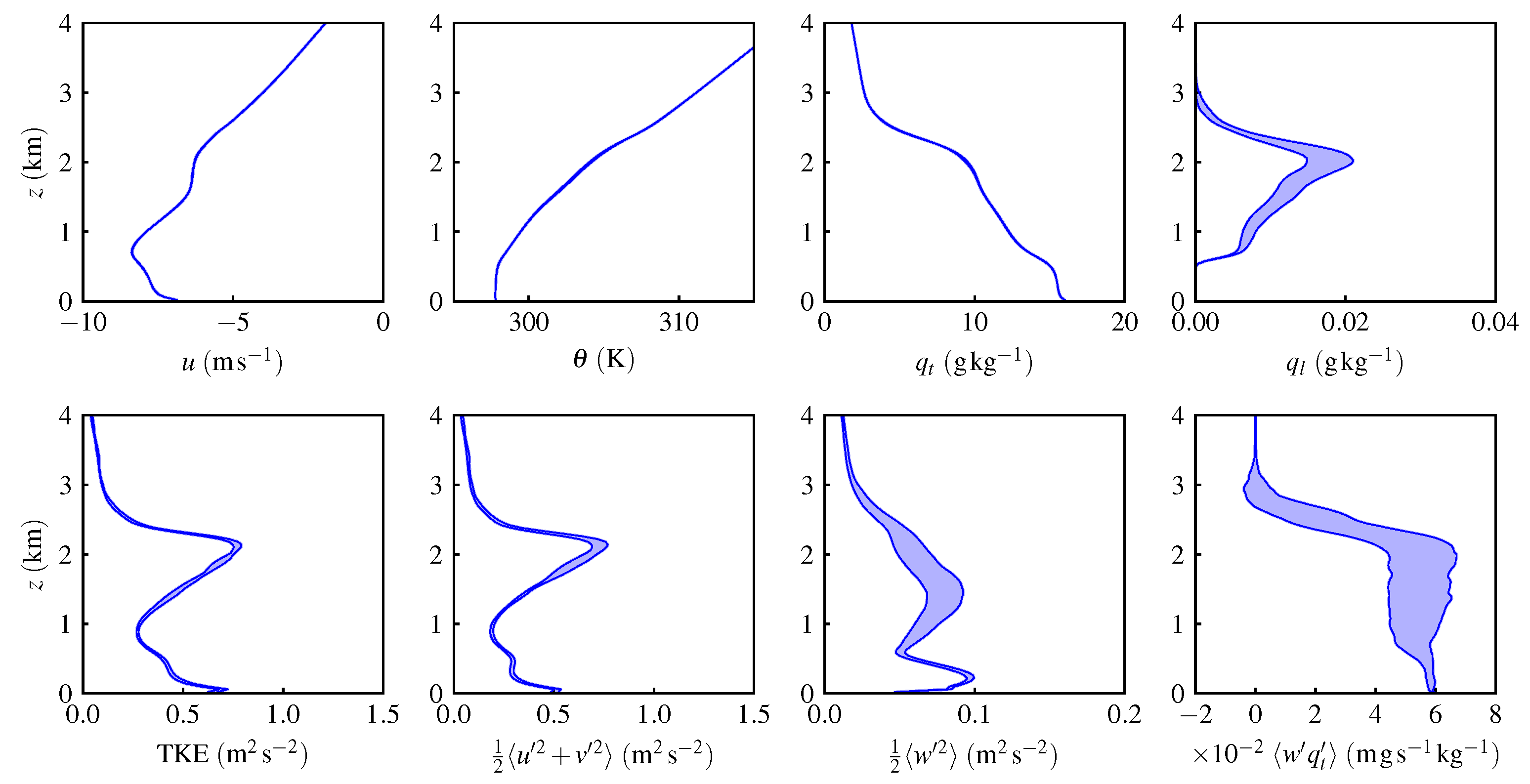
Figure A2.
Vertical profiles averaged in the horizontal directions and in time between t = 35–36 h for run B.
Figure A2.
Vertical profiles averaged in the horizontal directions and in time between t = 35–36 h for run B.
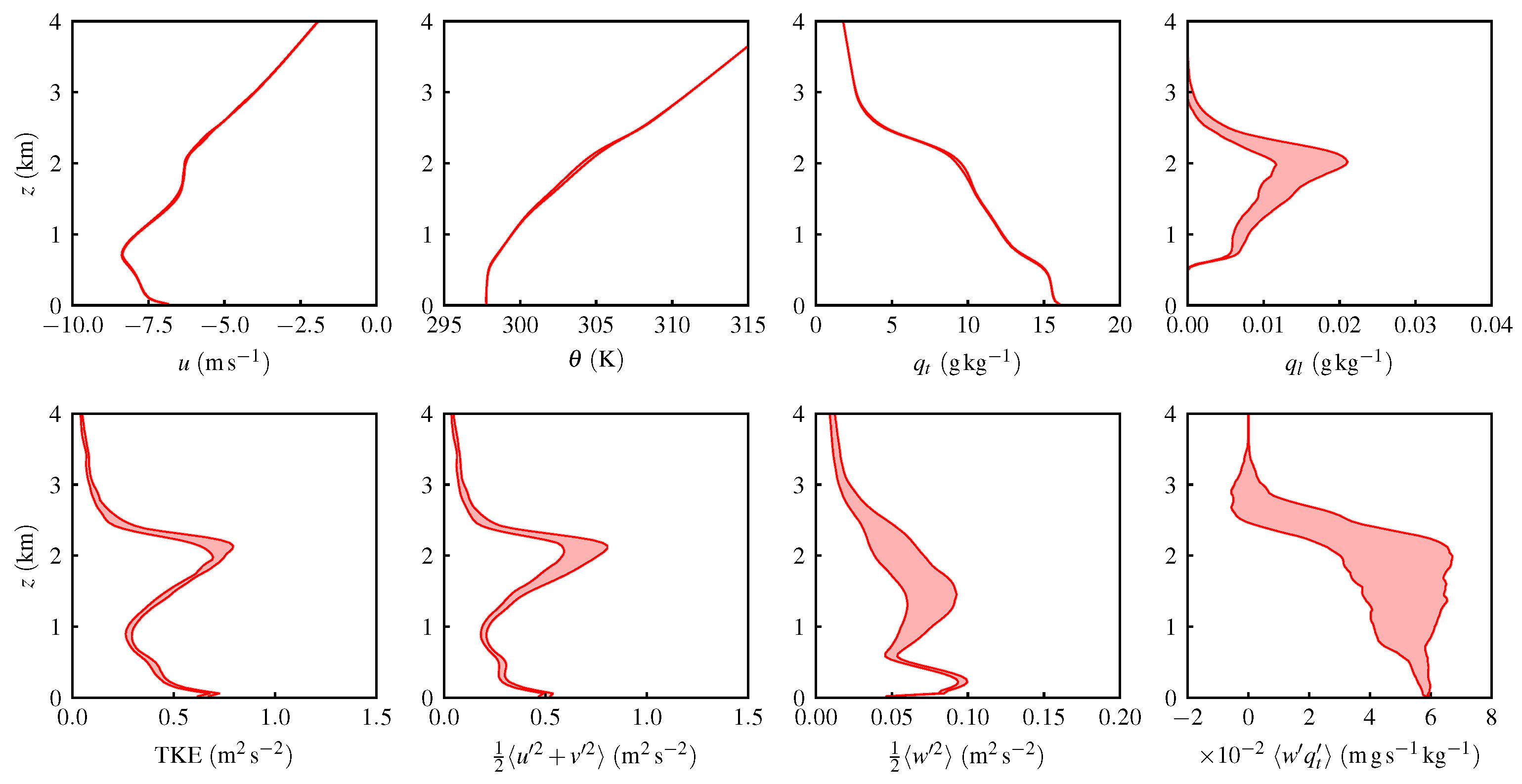
Figure A3.
Vertical profiles averaged in the horizontal directions and in time between t = 35–36 h for run C.
Figure A3.
Vertical profiles averaged in the horizontal directions and in time between t = 35–36 h for run C.
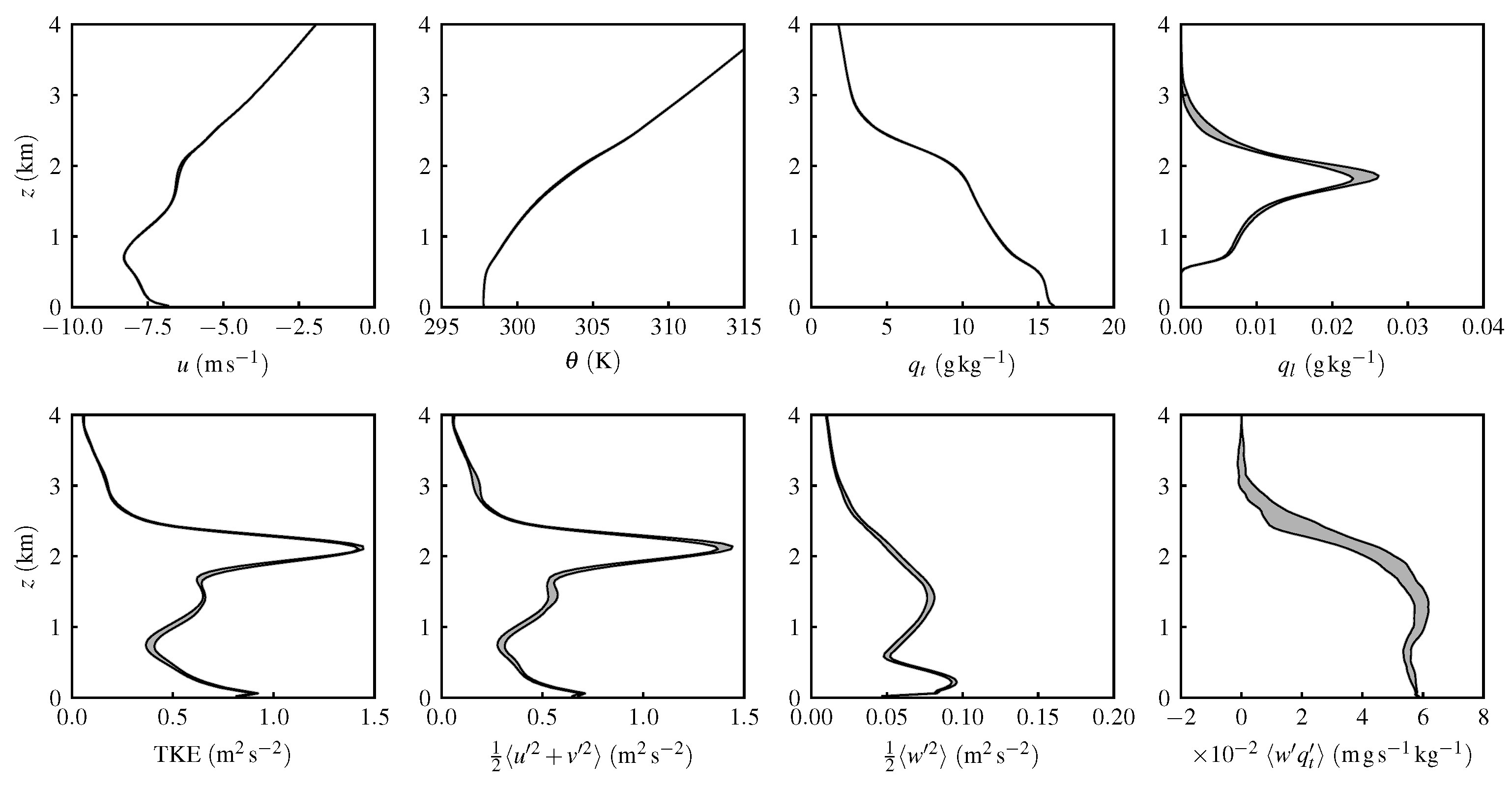
Figure A4.
Vertical profiles averaged in the horizontal directions and in time between t = 35–36 h for run D.
Figure A4.
Vertical profiles averaged in the horizontal directions and in time between t = 35–36 h for run D.

References
- Bony, S.; Stevens, B.; Frierson, D.M.; Jakob, C.; Kageyama, M.; Pincus, R.; Shepherd, T.G.; Sherwood, S.C.; Siebesma, A.P.; Sobel, A.H.; et al. Clouds, circulation and climate sensitivity. Nat. Geosci. 2015, 8, 261–268. [Google Scholar] [CrossRef] [Green Version]
- Zelinka, M.D.; Randall, D.A.; Webb, M.J.; Klein, S.A. Clearing clouds of uncertainty. Nat. Clim. Change 2017, 7, 674–678. [Google Scholar] [CrossRef]
- Klein, S.A.; Hall, A.; Norris, J.R.; Pincus, R. Low-Cloud Feedbacks from Cloud-Controlling Factors: A Review. In Shallow Clouds, Water Vapor, Circulation, and Climate Sensitivity; Pincus, R., Winker, D., Bony, S., Stevens, B., Eds.; Springer International Publishing: Cham, Switzerland, 2018; pp. 135–157. [Google Scholar]
- Savic-Jovcic, V.; Stevens, B. The structure and mesoscale organization of precipitating stratocumulus. J. Atmos. Sci. 2008, 65, 1587–1605. [Google Scholar] [CrossRef]
- LeMone, M.A.; Angevine, W.M.; Bretherton, C.S.; Chen, F.; Dudhia, J.; Fedorovich, E.; Katsaros, K.B.; Lenschow, D.H.; Mahrt, L.; Patton, E.G.; et al. 100 years of progress in boundary layer meteorology. Meteorol. Monogr. 2019, 59, 9.1–9.85. [Google Scholar] [CrossRef]
- Ovchinnikov, M.; Fast, J.D.; Berg, L.K.; Gustafson, W.I., Jr.; Chen, J.; Sakaguchi, K.; Xiao, H. Effects of horizontal resolution, domain size, boundary conditions, and surface heterogeneity on coarse LES of a convective boundary layer. Mon. Weather Rev. 2022, 150, 1397–1415. [Google Scholar] [CrossRef]
- Matheou, G.; Chung, D.; Nuijens, L.; Stevens, B.; Teixeira, J. On the fidelity of large-eddy simulation of shallow precipitating cumulus convection. Mon. Weather Rev. 2011, 139, 2918–2939. [Google Scholar] [CrossRef]
- Seifert, A.; Heus, T.; Pincus, R.; Stevens, B. Large-eddy simulation of the transient and near-equilibrium behavior of precipitating shallow convection. J. Adv. Model. Earth Syst. 2015, 7, 1918–1937. [Google Scholar] [CrossRef] [Green Version]
- Schalkwijk, J.; Jonker, H.J.J.; Siebesma, A.P.; Meijgaard, E.V. Weather forecasting using GPU-based large-eddy simulations. Bull. Am. Meteorol. Soc. 2015, 96, 715–723. [Google Scholar] [CrossRef] [Green Version]
- Anurose, T.; Bašták Ďurán, I.; Schmidli, J.; Seifert, A. Understanding the moisture variance in precipitating shallow cumulus convection. J. Geophys. Res.-Atmos. 2020, 125, e2019JD031178. [Google Scholar] [CrossRef] [Green Version]
- Lamaakel, O.; Matheou, G. Galilean invariance of shallow cumulus convection large-eddy simulation. J. Comput. Phys. 2021, 427, 11012. [Google Scholar] [CrossRef]
- Lamaakel, O.; Matheou, G. Organization development in precipitating shallow cumulus convection: Evolution of turbulence characteristics. J. Atmos. Sci. 2022, 79, 2419–2433. [Google Scholar] [CrossRef]
- Brown, A.R. The sensitivity of large-eddy simulations of shallow cumulus convection to resolution and subgrid model. Q. J. R. Meteorol. Soc. 1999, 125, 469–482. [Google Scholar] [CrossRef]
- De Roode, S.R.; Duynkerke, P.G.; Jonker, H.J. Large-eddy simulation: How large is large enough? J. Atmos. Sci. 2004, 61, 403–421. [Google Scholar] [CrossRef]
- Stevens, D.E.; Ackerman, A.S.; Bretherton, C.S. Effects of domain size and numerical resolution on the simulation of shallow cumulus convection. J. Atmos. Sci. 2002, 59, 3285–3301. [Google Scholar] [CrossRef]
- Cheng, A.; Xu, K.M.; Stevens, B. Effects of resolution on the simulation of boundary-layer clouds and the partition of kinetic energy to subgrid scales. J. Adv. Model. Earth Syst. 2010, 2, Art. #3. [Google Scholar] [CrossRef]
- Pedersen, J.G.; Malinowski, S.P.; Grabowski, W.W. Resolution and domain-size sensitivity in implicit large-eddy simulation of the stratocumulus-topped boundary layer. J. Adv. Model. Earth Syst. 2016, 8, 885–903. [Google Scholar] [CrossRef] [Green Version]
- Janssens, M.; De Arellano, J.V.G.; Van Heerwaarden, C.C.; De Roode, S.R.; Siebesma, A.P.; Glassmeier, F. Nonprecipitating shallow cumulus convection is intrinsically unstable to length scale growth. J. Atmos. Sci. 2023, 80, 849–870. [Google Scholar] [CrossRef]
- Seifert, A.; Heus, T. Large-eddy simulation of organized precipitating trade wind cumulus clouds. Atmos. Chem. Phys. 2013, 13, 5631–5645. [Google Scholar] [CrossRef] [Green Version]
- Dagan, G.; Koren, I.; Kostinski, A.; Altaratz, O. Organization and oscillations in simulated shallow convective clouds. J. Atmos. Sci. 2018, 10, 2287–2299. [Google Scholar] [CrossRef]
- Janssens, M.; Vilà-Guerau de Arellano, J.; Van Heerwaarden, C.C.; Van Stratum, B.J.; De Roode, S.R.; Siebesma, A.P.; Glassmeier, F. The time scale of shallow convective self-aggregation in large-eddy simulations Is sensitive to numerics. J. Adv. Model. Earth Syst. 2023, 15, e2022MS003292. [Google Scholar] [CrossRef]
- Matheou, G.; Chung, D. Large-eddy simulation of stratified turbulence. Part II: Application of the stretched-vortex model to the atmospheric boundary layer. J. Atmos. Sci. 2014, 71, 4439–4460. [Google Scholar] [CrossRef]
- Seifert, A.; Beheng, K.D. A double-moment parameterization for simulating autoconversion, accretion and selfcollection. Atmos. Res. 2001, 59–60, 265–281. [Google Scholar] [CrossRef]
- Chung, D.; Matheou, G. Large-eddy simulation of stratified turbulence. Part I: A vortex-based subgrid-scale model. J. Atmos. Sci. 2014, 71, 1863–1879. [Google Scholar] [CrossRef]
- Morinishi, Y.; Lund, T.S.; Vasilyev, O.V.; Moin, P. Fully conservative higher order finite difference schemes for incompressible flow. J. Comput. Phys. 1998, 143, 90–124. [Google Scholar] [CrossRef] [Green Version]
- Spalart, P.R.; Moser, R.D.; Rogers, M.M. Spectral methods for the Navier–Stokes equations with one infinite and two periodic directions. J. Comput. Phys. 1991, 96, 297–324. [Google Scholar] [CrossRef]
- Rauber, R.M.; Stevens, B.; Ochs, H.T., III; Knight, C.; Albrecht, B.A.; Blyth, A.M.; Fairall, C.W.; Jensen, J.B.; Lasher-Trapp, S.G.; Mayol-Bracero, O.L.; et al. Rain in shallow cumulus over the ocean: The RICO campaign. Bull. Am. Meteorol. Soc. 2007, 88, 1912–1928. [Google Scholar] [CrossRef] [Green Version]
- van Zanten, M.C.; Stevens, B.; Nuijens, L.; Siebesma, A.P.; Ackerman, A.S.; Burnet, F.; Cheng, A.; Couvreux, F.; Jiang, H.; Khairoutdinov, M.; et al. Controls on precipitation and cloudiness in simulations of trade-wind cumulus as observed during RICO. J. Adv. Model. Earth Syst. 2011, 3, M06001. [Google Scholar]
- Nuijens, L.; Stevens, B.; Siebesma, A.P. The environment of precipitating shallow cumulus convection. J. Atmos. Sci. 2009, 66, 1962–1979. [Google Scholar] [CrossRef] [Green Version]
- Snodgrass, E.R.; Di Girolamo, L.; Rauber, R.M. Precipitation characteristics of trade wind clouds during RICO derived from radar, satellite, and aircraft measurements. J. Appl. Meteorol. 2009, 48, 464–483. [Google Scholar] [CrossRef]
- Li, Z.; Zuidema, P.; Zhu, P. Simulated convective invigoration processes at trade wind cumulus cold pool boundaries. J. Atmos. Sci. 2014, 71, 2823–2841. [Google Scholar] [CrossRef]
- Inoue, M.; Matheou, G.; Teixeira, J. LES of a spatially developing atmospheric boundary layer: Application of a fringe method for the stratocumulus to shallow cumulus cloud transition. Mon. Weather Rev. 2014, 142, 3418–3424. [Google Scholar] [CrossRef]
- Matheou, G.; Bowman, K.W. A recycling method for the large-eddy simulation of plumes in the atmospheric boundary layer. Environ. Fluid Mech. 2016, 16, 69–85. [Google Scholar] [CrossRef]
- Matheou, G. Numerical discretization and subgrid-scale model effects on large-eddy simulations of a stable boundary layer. Q. J. R. Meteorol. Soc. 2016, 142, 3050–3062. [Google Scholar] [CrossRef]
- Thorpe, A.K.; Frankenberg, C.; Green, R.O.; Thompson, D.R.; Aubrey, A.D.; Mouroulis, P.; Eastwood, M.L.; Matheou, G. The Airborne Methane Plume Spectrometer (AMPS): Quantitative imaging of methane plumes in real time. In Proceedings of the 2016 IEEE Aerospace Conference, Big Sky, MT, USA, 5–12 March 2016; pp. 1–14. [Google Scholar]
- Jongaramrungruang, S.; Frankenberg, C.; Matheou, G.; Thorpe, A.K.; Thompson, D.R.; Kuai, L.; Duren, R.M. Towards accurate methane point-source quantification from high-resolution 2-D plume imagery. Atmos. Meas. Tech. 2019, 12, 6667–6681. [Google Scholar] [CrossRef] [Green Version]
- Couvreux, F.; Bazile, E.; Rodier, Q.; Maronga, B.; Matheou, G.; Chinita, M.J.; Edwards, J.; Stratum, B.J.H.V.; Heerwaarden, C.C.V.; Huang, J.; et al. The GABLS4 experiment: Intercomparison of large-eddy simulation models of the antarctic boundary layer challenged by very stable stratification. Bound.-Layer Meteorol. 2020, 176, 369–400. [Google Scholar] [CrossRef]
- Hunter, J.D. Matplotlib: A 2D graphics environment. Comput. Sci. Eng. 2007, 9, 90–95. [Google Scholar] [CrossRef]
Figure 1.
LES domain sizes and cloud liquid water path (LWP) at the end of the run, . The computational domain area quadruples as the LES computational domain increases. Axes ticks correspond to 50-km intervals. Axes labels are not shown to maximize the plot area.
Figure 1.
LES domain sizes and cloud liquid water path (LWP) at the end of the run, . The computational domain area quadruples as the LES computational domain increases. Axes ticks correspond to 50-km intervals. Axes labels are not shown to maximize the plot area.
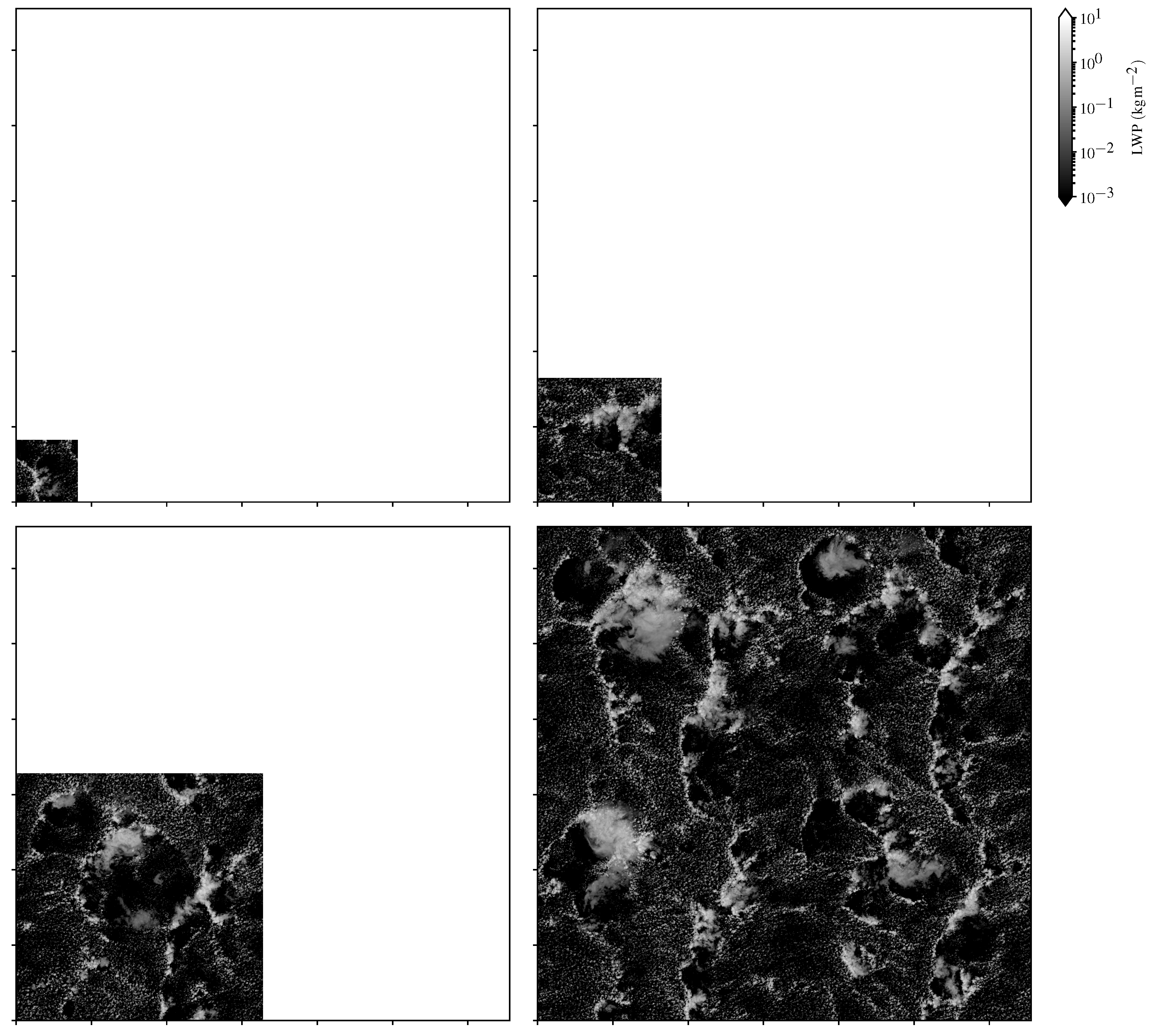
Figure 2.
Rain water path (RWP) at . Axes ticks correspond to 50-km intervals. Axes labels are not shown to maximize the plot area. See Figure 1 for the corresponding LWP field.
Figure 2.
Rain water path (RWP) at . Axes ticks correspond to 50-km intervals. Axes labels are not shown to maximize the plot area. See Figure 1 for the corresponding LWP field.

Figure 3.
Evolution of vertically integrated turbulent kinetic energy (VTKE), cloud-liquid water path (LWP), rain water path (RWP), cloud base , cloud top height , inversion height , cloud cover and surface precipitation rate.
Figure 3.
Evolution of vertically integrated turbulent kinetic energy (VTKE), cloud-liquid water path (LWP), rain water path (RWP), cloud base , cloud top height , inversion height , cloud cover and surface precipitation rate.

Figure 4.
Profiles of (a) u-component wind, (b) potential temperature , (c) total water mixing ratio , (d) cloud liquid water mixing ratio , (e) turbulent kinetic energy (TKE), (f) horizontal component of TKE, (g) vertical velocity variance and (h) vertical total water flux at the end of the LES runs, .
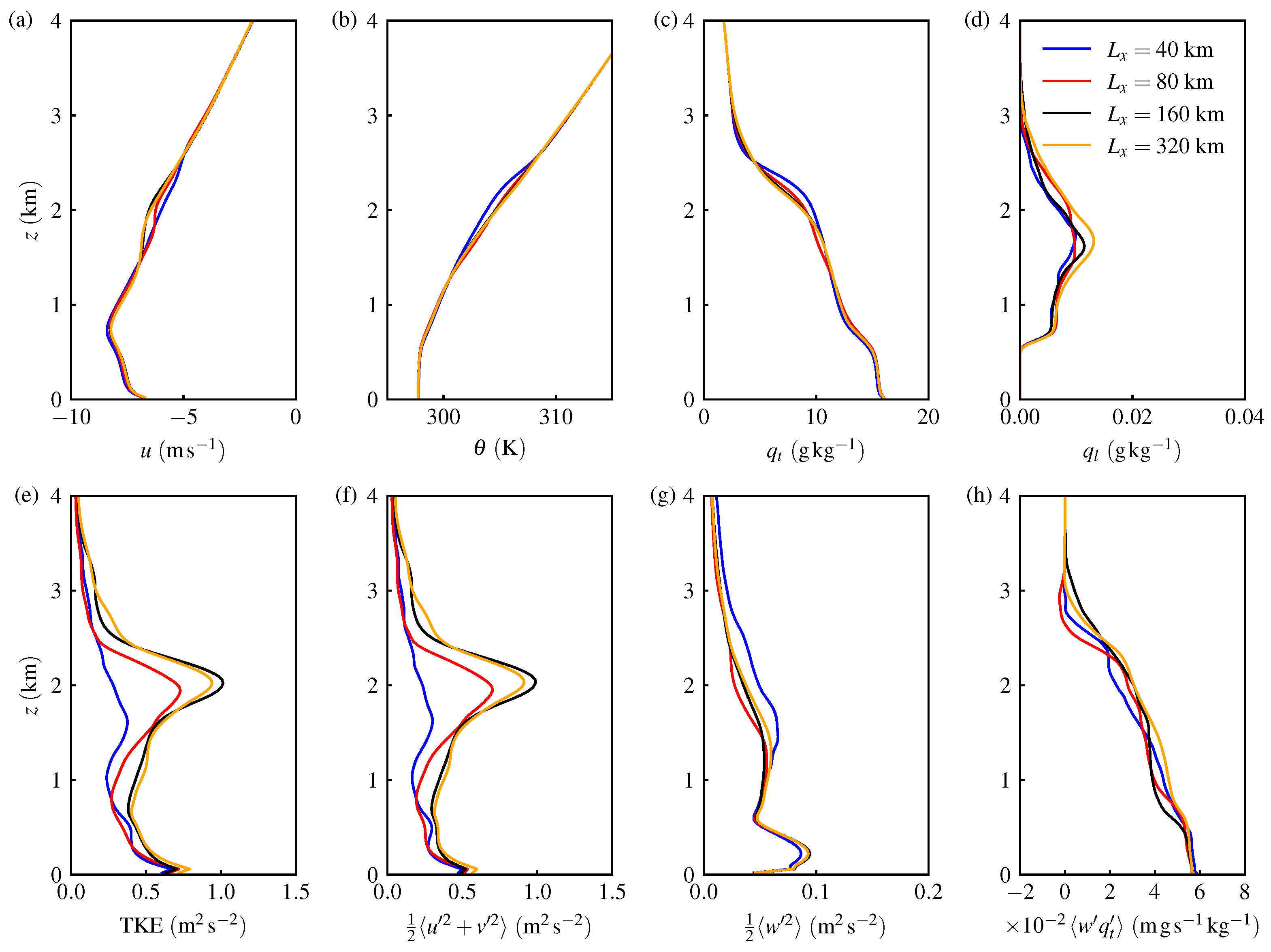
Figure 5.
(a) Resolved-scale total water mixing ratio, and (b) liquid water potential temperature variance at for all LES domains.
Figure 5.
(a) Resolved-scale total water mixing ratio, and (b) liquid water potential temperature variance at for all LES domains.
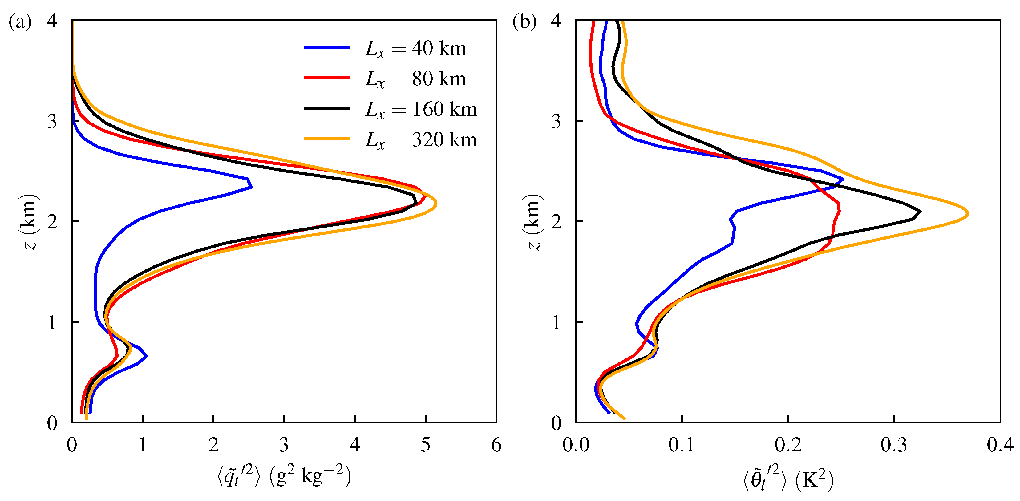
Figure 6.
(a) Time evolution of inversion strength for all runs. (b) Inversion height and inversion strength in the subdomains of run D at with open circles. Filled circle corresponds to the entire-domain average, which is the same value as the line for run D at of (a).
Figure 6.
(a) Time evolution of inversion strength for all runs. (b) Inversion height and inversion strength in the subdomains of run D at with open circles. Filled circle corresponds to the entire-domain average, which is the same value as the line for run D at of (a).
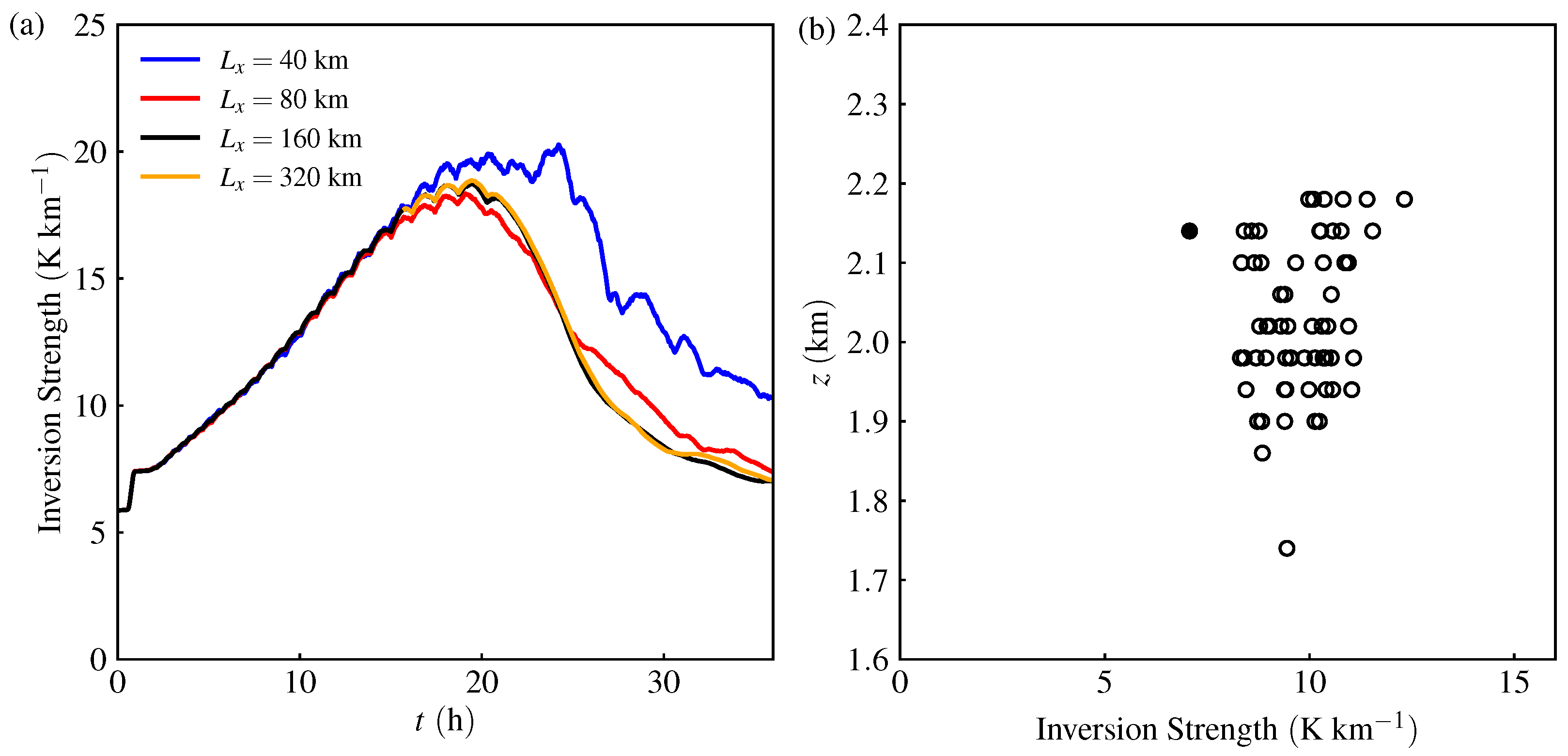
Figure 7.
Premultiplied one-dimensional spectra. All spectra are computed at along the zonal direction. The x-axis is converted to length scale to assist the physical interpretation. In each panel, spectra from all four runs are shown, lines are as in Figure 4. Panel rows from top to bottom correspond to a different time (a–d), 30 (e–h) and (i–l). In each row, panels correspond to different variables: from left to right, zonal wind, vertical velocity, liquid water potential temperature, and total water mixing ratio.
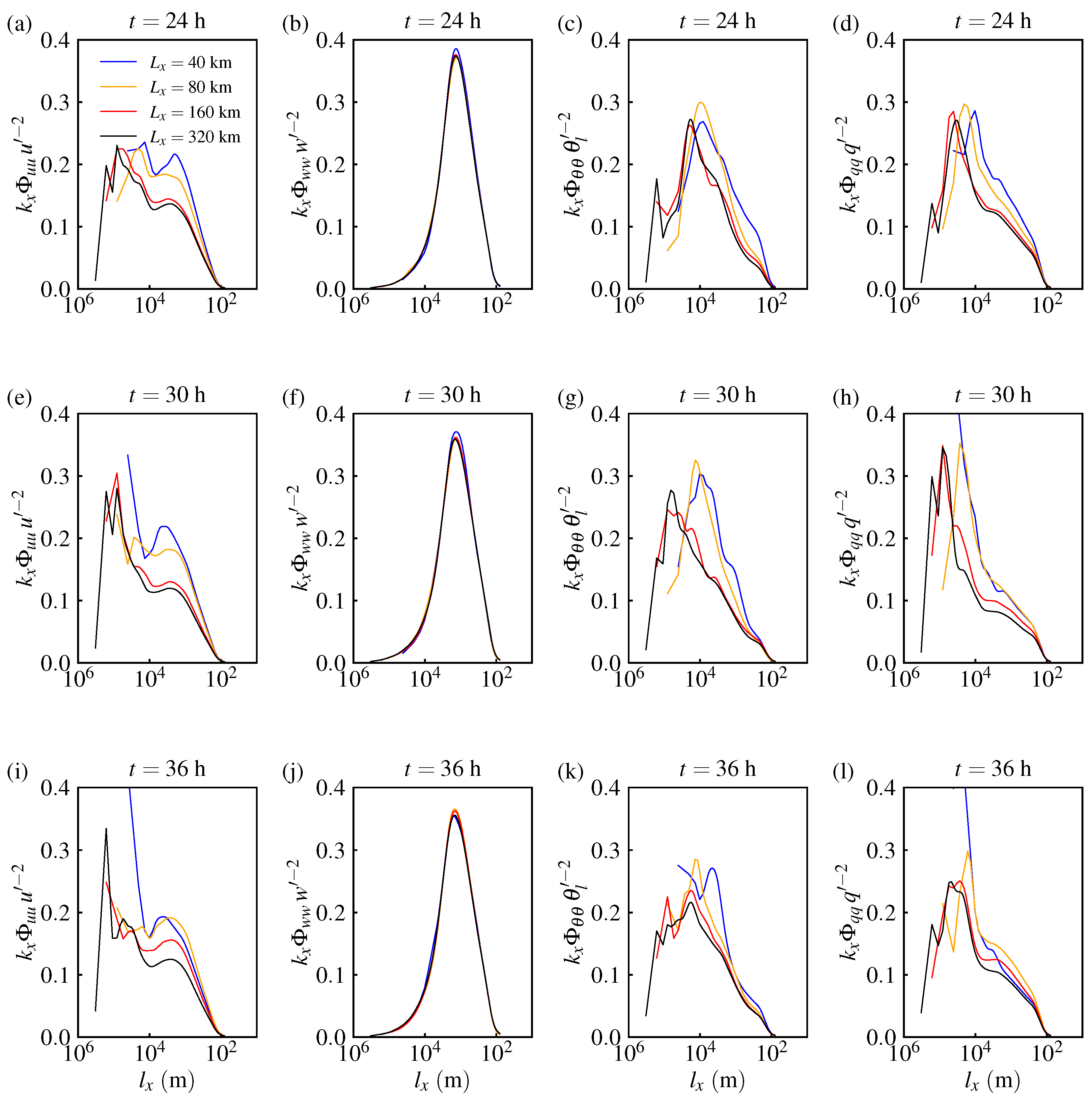
Figure 8.
Horizontal length scales computed from runs C (black symbols) and D (orange). (a) Length scales of zonal wind . (b) Meridional wind . (c) Liquid water potential temperature . (d) Total water mixing ratio and radii of two cold pools and from run C. (e) Vertical velocity .
Figure 8.
Horizontal length scales computed from runs C (black symbols) and D (orange). (a) Length scales of zonal wind . (b) Meridional wind . (c) Liquid water potential temperature . (d) Total water mixing ratio and radii of two cold pools and from run C. (e) Vertical velocity .

Table 1.
Details of the large-eddy simulations. The number of grid points in the meridional x and zonal y directions is and the number of vertical grid points is . The grid spacing is isotropic . All domains are square in the horizontal directions with extents . The height of the computational domain is .
| Run | |||||
|---|---|---|---|---|---|
| A | 1024 | 125 | 40.96 | 5 | 40 |
| B | 2048 | 125 | 80.92 | 5 | 40 |
| C | 4096 | 125 | 163.84 | 5 | 40 |
| D | 8192 | 125 | 327.68 | 5 | 40 |
Disclaimer/Publisher’s Note: The statements, opinions and data contained in all publications are solely those of the individual author(s) and contributor(s) and not of MDPI and/or the editor(s). MDPI and/or the editor(s) disclaim responsibility for any injury to people or property resulting from any ideas, methods, instructions or products referred to in the content. |
© 2023 by the authors. Licensee MDPI, Basel, Switzerland. This article is an open access article distributed under the terms and conditions of the Creative Commons Attribution (CC BY) license (https://creativecommons.org/licenses/by/4.0/).
Share and Cite
MDPI and ACS Style
Lamaakel, O.; Venters, R.; Teixeira, J.; Matheou, G. Computational Domain Size Effects on Large-Eddy Simulations of Precipitating Shallow Cumulus Convection. Atmosphere 2023, 14, 1186. https://doi.org/10.3390/atmos14071186
AMA Style
Lamaakel O, Venters R, Teixeira J, Matheou G. Computational Domain Size Effects on Large-Eddy Simulations of Precipitating Shallow Cumulus Convection. Atmosphere. 2023; 14(7):1186. https://doi.org/10.3390/atmos14071186
Chicago/Turabian StyleLamaakel, Oumaima, Ravon Venters, Joao Teixeira, and Georgios Matheou. 2023. "Computational Domain Size Effects on Large-Eddy Simulations of Precipitating Shallow Cumulus Convection" Atmosphere 14, no. 7: 1186. https://doi.org/10.3390/atmos14071186
Note that from the first issue of 2016, this journal uses article numbers instead of page numbers. See further details here.