Article

Subseasonal Variation Characteristics of Low-Cloud Fraction in Southeastern and Northwestern North Pacific

1
Zhoushan Meteorological Bureau, Zhoushan 316000, China
2
Key Laboratory of Meteorological Disaster, Ministry of Education, Joint International Research Laboratory of Climate and Environment Change, Collaborative Innovation Center on Forecast and Evaluation of Meteorological Disasters, Nanjing University of Information Science & Technology, Nanjing 210044, China
3
School of Atmospheric Sciences, Nanjing University of Information Science & Technology, Nanjing 210044, China
*
Author to whom correspondence should be addressed.
Atmosphere 2023, 14(11), 1668; https://doi.org/10.3390/atmos14111668
Submission received: 15 September 2023 / Revised: 25 October 2023 / Accepted: 7 November 2023 / Published: 10 November 2023
(This article belongs to the Section Meteorology)

Abstract

:
The subseasonal variability of the low-cloud fraction (LCF) over the southeastern North Pacific (SENP) and northwestern North Pacific (NWNP) was studied using satellite observations and the European Centre for Medium-Range Weather Forecasts (ECMWF) reanalysis. It is found that subseasonal variability of the LCF was closely related to variations in the estimated inversion strength (EIS), sea surface wind speed (SSW), sensible heat flux (SHF), sea surface temperature (SST), surface temperature advection (Tadv), relative humidity (RH), surface level pressure (SLP) and surface air temperature (SAT). An increase in the LCF over the SENP is associated with the development of an anomalous anticyclonic circulation, which is located on the west coast of America. The cold advection, together with the subsidence warming associated with the anticyclonic circulation, strengthens the temperature inversion, favoring the development of the LCF. In the NWNP, the maximum LCF anomaly was also correlated with the stable boundary layer. The southerly wind blows airflow over the Kuroshio Extension from the subtropics, which brings warm and moist air. When air flows to the colder sea surface, it is cooled and condensed by the intensified heat exchange. A lead-lag composite analysis indicates that the mechanisms are different between the SENP and the NWNP, possibly due to the different types of low-level clouds over these two regions. In the SENP, the trade cumulus dominates under a strong capping inversion over the subtropics, whereas fog and stratus often occur under a shallow capping inversion in the NWNP. The effects of atmospheric circulation are also discussed.

1. Introduction

Low-level clouds are very important to the regional and global climate because they reflect longwave and shortwave radiation from the atmosphere [1]. Small changes in the low-cloud fraction (LCF) will significantly influence the weather and climate [2]. For example, Xie found that the low-level cloud deck over the subtropical southeast Pacific reduces the incoming solar radiation at the sea surface and cools the local sea surface temperature (SST), triggering a coupled ocean–atmospheric adjustment that strengthens the climatic asymmetry in both east–west and north–south directions across the basin [3]. Oreopoulos [4] found that low-level clouds have had a positive effect on global warming in recent years. Thus, it is crucial to investigate the variation in low-level clouds and the associated meteorological parameters [5].
Previous studies on the variability of low-level clouds have focused on their seasonal mean properties on the basis of surface-based observations. These studies have shown that, on seasonal and interannual time scales, atmospheric circulation has significant effects on the variations in LCF, sea surface temperature (SST), and tropospheric stability. They pointed out that there is a negative correlation between LCF and SST anomalies: colder SST anomalies can increase the lower tropospheric stability and thus low-cloud amount, which in turn further cools the SST [6,7,8,9,10]. On smaller spatial scales, the correlation between the LCF and SST anomalies may become positive. On these scales, relative humidity (RH) plays an important role in the promotion of low-level clouds [11].
On shorter timescales (diurnal and synoptic time scales), the variability of LCF has also been studied well. Previous studies have shown that variations in LCF on timescales greater than one day but less than a month are closely coupled with atmospheric circulation, SST, and the stability of the lower troposphere [12]. They also found that synoptic variations of LCF are strongly correlated with surface temperature advection (Tadv), the lower tropospheric stability, and the RH at the cloud layer [13]. Wylie et al. [14] found that increases in the LCF were statistically related to increased cold advection in the planetary boundary layer (PBL) and 500-hPa geopotential height and decreased boundary layer depth.
The subseasonal timescale is defined as the timescale shorter than the seasonal timescale but longer than the diurnal timescale. In comparison to other timescales, the subseasonal variability of the LCF has been rarely studied despite its importance for climate. A strong correlation was observed between the intraseasonal variability of the South Asian monsoon and the Indo–Pacific SST, which has positive feedback with low-level clouds [15,16]. Xu et al. [17] pointed out that subseasonal LCF has considerable variability in two-week and 40–80-day bands in association with cold Tadv in the PBL. In the subtropical southeastern Pacific, the subseasonal variation of the LCF is largely affected by sea surface wind speed (SSW), surface air temperature (SAT), sensible heat flux (SHF), and SSTs. Previous studies have focused on low-level clouds in the eastern coastal areas. When it comes to the open oceans, such as the mid-latitudes of the Northwestern Pacific, our knowledge is lacking. The atmospheric circulation is different in different areas of the Pacific; specifically, in the eastern North Pacific, the atmosphere is usually controlled by the Subtropical High, while the upper-level trough is frequently found in the western North Pacific; besides, the Kuroshio extensions occur in the northwestern Pacific [18,19,20]. In this study, our efforts are especially paid to the subseasonal variations of the LCF over the southeastern (SENP) and northwestern North Pacific (NWNP), as well as differences in their associated controlling factors. Such a critical analysis may help improve atmospheric general circulation models, which tend to underestimate the amount of low clouds over the oceans.
The rest of this paper is organized as follows. In Section 2, we introduced the data and the methods used in this study. Section 3.1 investigates the subseasonal variation characteristics of the LCF over SENP and NWNP. The controlling factors are examined in Section 3.2. In Section 3.3, the lead-lag relationship between LCF and its associated controlling factors is explored, as well as the relationship between subseasonal LCF variation and large-scale circulation. The conclusions and discussion are presented in Section 4.

2. Data and Methods

2.1. Reanalysis Data

ERA5 is the fifth generation European Centre for Medium-range Weather Forecasts (ECMWF) atmospheric reanalysis of the global climate, covering the period from January 1940 to the present. In this study, we use the daily averaged ERA5 reanalysis data on a 1° × 1° grid, including vertical velocity (ɷ), RH, 700-hPa geopotential height ( Z 700 ), SAT, SST, dew-point temperature (Td), SSW, and sea level pressure (SLP) [21,22].
In addition, we used the daily averaged SHF and surface latent heat flux (LHF) obtained from the Woods Hole Oceanographic Institution (WHOI) [22] on a 1° × 1° grid. The meteorological parameters used in this study were measured between January 2011 and December 2015.

2.2. Satellite Data

The satellite observations offer a high-resolution view of the vast oceans and overlying atmosphere in detail never possible before [23,24]. In this study, we used the daily cloud product of the Moderate Resolution Imaging Spectroradiometer (MODIS). The MODIS cloud product combines infrared and visible techniques to determine both the physical and radiative cloud properties. Daily global Level 2 data were provided. The cloud fraction was produced by the infrared retrieval methods both day and night at a 5 km × 5 km pixel resolution. The MODIS Cloud Product includes the cirrus reflectance in the visible at the 1-km-pixel resolution, which is useful for removing cirrus scattering effects from the land-surface reflectance product. The MODIS cloud product includes the cloud fraction and cloud-top pressure. In this study, clouds with top pressures higher than 680-hPa were defined as low-level clouds [25,26]. To be consistent with the reanalysis data, we used the daily averaged ERA5 reanalysis data on a 1° × 1° grid. The cloud data were collected between January 2011 and December 2015. During this period, there were no specific climatic events or phenomena (e.g., El Niño) that might have influenced the study outcomes.

2.3. Calculated Data

From the sounding data, several quantities can be calculated. First, the estimated inversion strength (EIS) was estimated using the following algorithm, which takes advantage of the fact that the trade inversion is a layer typified by a rise in temperature with height and a drop in relative humidity with height. EIS is a modification of lower-tropospheric stability (LTS) [8], which is a more plausible and useful index than LTS for determining low cloud cover (LCC) in the present climate. The calculation formula is as follows [27]:
EIS = ( θ 700 θ sfc ) γ m 850 ( Z 700 Z L C L )
In this formula, θ 700 and θ sfc respectively represent the potential temperatures at 700-hPa and surface. Z 700 and Z L C L represent the height at 700-hPa and lifting condensation level. Besides, γ m 850 is the vertical decline rate of temperature at 850-hPa. The calculation formula of Z L C L is as follows:
Z L C L = 123 × ( SAT Td )
In addition, the sea surface temperature advection (Tadv) is determined from the slopes derived from ERA5 data with the surface wind. This is a reasonable approximation if the air temperature does not differ too significantly from the SST and if the SST gradient remains relatively constant over a month. The values were calculated using the following formula:
Tadv = V s f c × SST
In this formula, Vsfc represents the surface winds, and ∇SST represents the horizontal SST gradient [28].

2.4. Methods

In previous studies, the annual and semiannual harmonics were used to represent the seasonal cycle, and subseasonal anomalies were defined as deviations from this seasonal cycle plus the multi-year mean [17]. In this study, we use the band-pass filters in NCL (https://www.ncl.ucar.edu/Document/Functions/Built-in/filwgts_lanczos.shtml, (accessed on 5 September 2022)) to get the subseasonal signal of satellite data and reanalysis data. In this function, the total number of weights (nwt) was set to 201, and the cutoff frequency of the ideal band-pass filter was set to fca = 1/90, and fcb = 1/10. This means that a subseasonal signal between 10–90 days was selected. Note that the higher the weights, the better the filter; however, there is a greater loss of data.
A Morlet wavelet was applied to obtain the local wavelet power spectrum of the LCF time-series [17]. In this study, we use the wavelet function in NCL (https://www.ncl.ucar.edu/Document/Functions/Built-in/wavelet.shtml, (accessed on 5 September 2022)) to calculate the wavelet transform of a time series and significance levels. The wavelet analysis can detect any detail of a signal by localized analysis in time and space and has been widely used [29].
In assessing the significance of correlations between two variables (e.g., x and y), the number of independent paired observations is required. This number is assigned as the length of the observations divided by the maximum of x and y. The significance was then determined using a standard t-test with the correlation coefficient, the number of independent paired observations, and a specified confidence level. In this study, we used the t-test to investigate the significance of the correlation.
Composite analysis involves collecting a large number of cases of a given meteorological phenomenon. It may be necessary to standardize the cases in some fashion; then, these cases are composited together as a collection, perhaps with different types of stratification using one or more covariates that are suspected of having an influence on the phenomenon. The composite analysis generally involves computing the composite mean and perhaps computing some other statistical measures, such as the standard deviation and statistical significance. If done properly, the resulting structures that emerge can tell a powerful story about how the meteorological phenomenon is affected by the factors used in the composite stratification. In this study, we used composite analysis to calculate how the subseasonal variations were affected by meteorological parameters [30,31].

3. Results

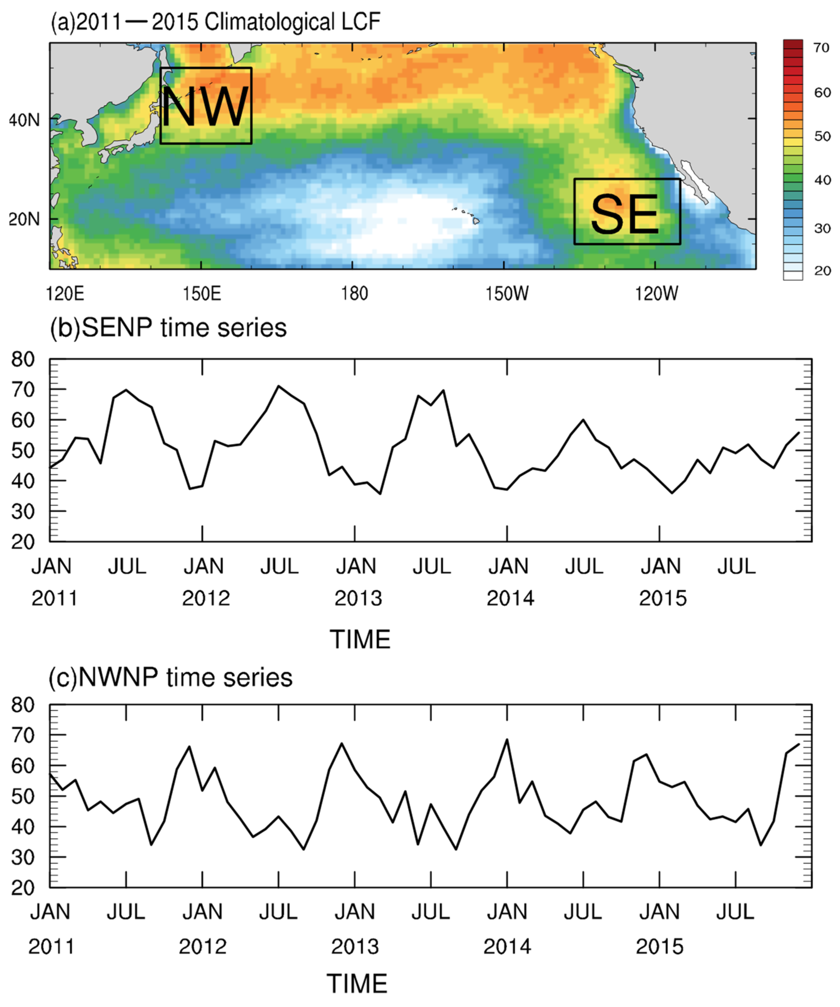
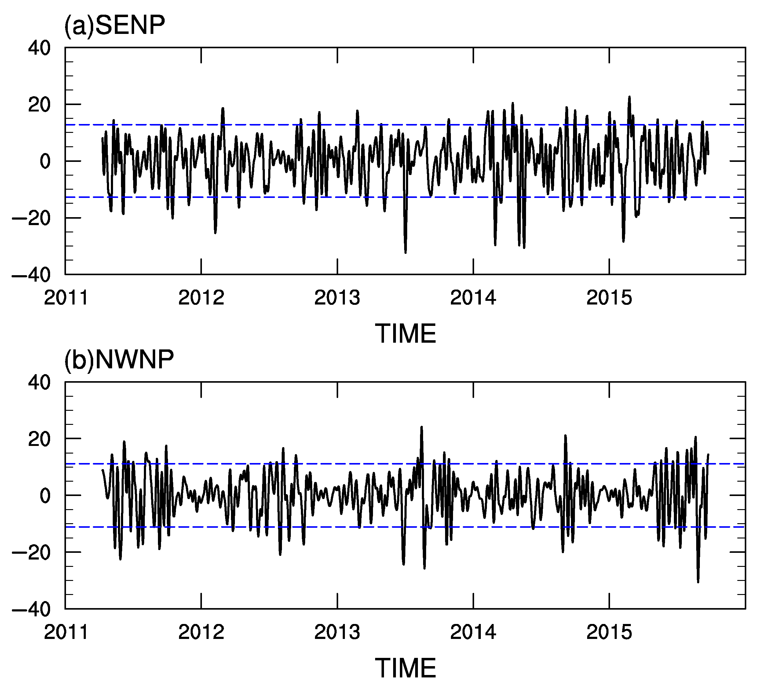
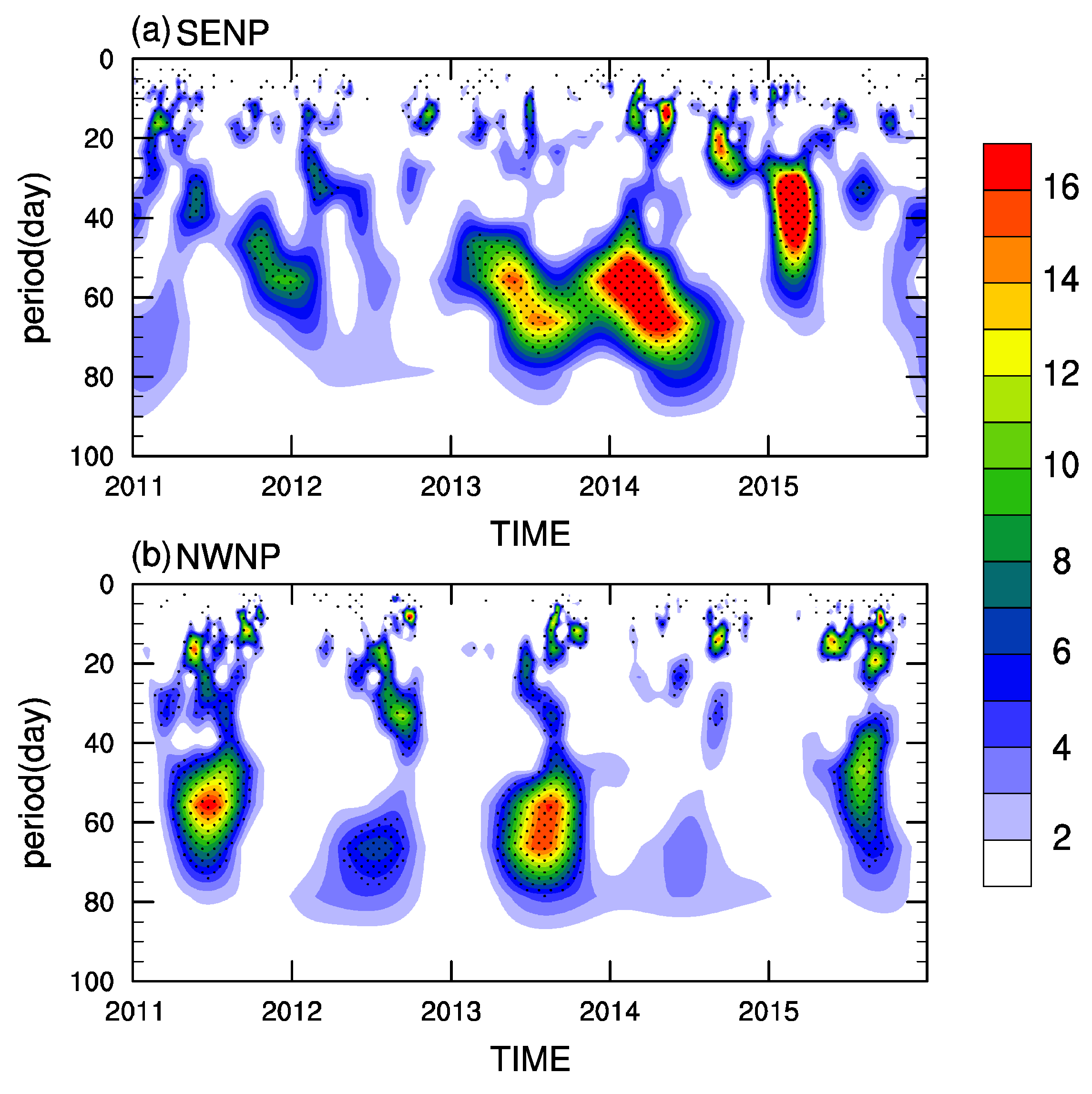
3.1. Subseasonal Variation of LCF

Figure 1a shows the spatial distribution of the 5-year (2011–2015) mean LCF in the North Pacific. Large LCF is located in the subtropical northeast Pacific, Bering Sea, and the ocean near the Kuril Islands. Here, we focus on the southeastern North Pacific (SENP; 115–136° W, 15–28° N) and the northwestern Pacific (NWNP; 142–160° E, 35–50° N).
The monthly LCF over the SENP and the NWNP had an obvious annual cycle. In the SENP, the maximum LCF was in summer, and the minimum in winter (Figure 1b). The annual cycle of the NWNP is completely opposite, with a maximum in winter and a minimum in summer (Figure 1c). In this study, the seasonal cycle is defined as annual and semiannual harmonics, while the subseasonal anomalies are the deviations from this seasonal cycle plus the 5-year (2011–2015) mean.
Figure 2 shows the evolution of LCF anomalies averaged over the SENP (Figure 2a) and NWNP (Figure 2b) regions from 2011 to 2015. There is considerable subseasonal variability in the LCF over these two regions. Further analysis of the Morlet wavelet (Figure 3) showed the strongest LCF oscillations at approximately 8–16 days and 40–80 days. The LCF spectrum in SENP has a significant 50–70 day-peak from late spring of 2013 to the summer of 2014, and a 30–50 day-peak occurs at the beginning of 2015. In the NWNP, the LCF spectrum has a significant 50–70 day-peak in the late summer and early fall of 2011 and 2013 and a 40–60 day-peak in the fall of 2015.

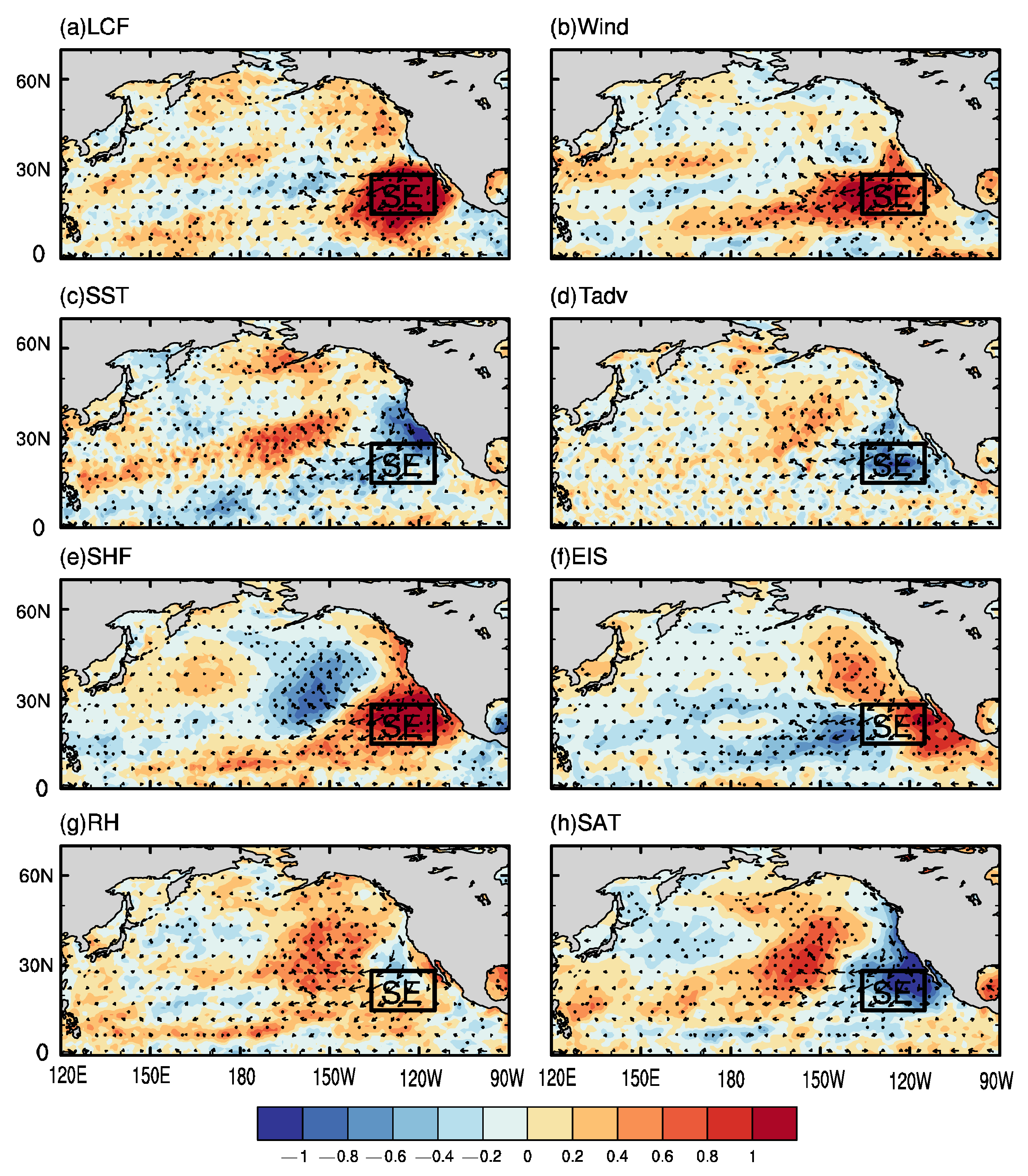
3.2. Association with Meteorological Parameters

To further examine the relationship between surface meteorological variables and LCF in the SENP and NWNP regions, Figure 4 shows the correlation coefficients between LCF and other variables. In the SENP, there was a positive correlation between the LCF and SSW, which is consistent with the previous findings in the northeast Pacific [13]. Besides, we found that LCF is highly negatively correlated with Tadv and SAT due to the cold advection (Figure 4a). Thus, the colder SAT anomalies and anomalous subsidence (i.e., increased ω 700 ) would increase the stability of the boundary layer (estimated by EIS); that is, EIS is positively correlated with LCF variations. The enhanced temperature inversion inhibited cloud-top entrainment of dry air, thus further increasing the LCF.
The LCF showed the most significant correlation with the SHF. Due to the decreased SAT and increased surface wind, both SHF and LHF increases are positively correlated with LCF variations [32,33]. In addition, the RH was negatively correlated with the LCF in the SENP, indicating the cold and dry advection, although their correlation was less significant. Surface humidity anomalies are quite weak or do not even exist, which may be due to the competition between wetting caused by increased surface flux and drying caused by enhanced horizontal advection and vertical mixing [17].
In the NWNP, the relationship between the surface meteorological variables and the LCF was different from that in the SENP (Figure 4b). There was no significant correlation between the LCF and SHF, which means that LCF variations in the NWNP were affected by other variables. SAT and LCF were positively correlated due to the warm advection and the strengthened surface southerly winds, whereas the SST only showed a slightly positive correlation with LCF. The warmer the SAT and colder SST are beneficial for the stability of the air-sea interface (as estimated by EIS) and further contribute to the formation of low clouds.
Furthermore, RH showed the most significant correlation with the LCF in the NWNP. The significant positive correlation between cloud amount and the RH is consistent with the results of Slingo and Bretherton [34,35]. They found that for a persistent large-scale stratiform cloud, the RH at the level of the cloud must be close to 100%. A large amount of moisture was transported northward by the southerlies to form low clouds. In addition, there is a highly negative correlation between the LCF and SLP, indicating that the subseasonal variation in LCF is also related to large-scale circulation.
To examine the correlation between the large-scale circulation and the LCF, we composite SSW, SST, Tadv, SHF, EIS, SAT, and RH based on the time series of area-averaged LCF in the SENP and the NWNP, respectively (Figure 2). The positive (negative) LCF phases are defined as those with an LCF index above 1.5 (below −1.5) standard deviations. In the SENP, there were 69 and 142 days in the 5-yr data record for the positive and negative LCF phases, respectively. In the NWNP, there were 75 and 133 days, respectively. Composite fields were separately averaged over these days for positive and negative phases. Thus, the differences in the composite fields between the positive and negative phases are discussed in the following.
Figure 5 presents the composite differences of LCF, SSW, SST, Tadv, SHF, SAT, RH, and EIS in the SENP. It is found that the increased LCF was associated with an anomalous anticyclonic circulation centered near 40° N, 135° W (Figure 5a). In Figure 5, the correlation between the LCF and SLP is only slightly positive in the SENP due to the positional abnormality between the anticyclone center and the maximum LCF anomaly. The northeasterly trades act to enhance SSW in the southern part of this anomalous anticyclonic circulation (Figure 5b), consistent with the positive LCF-SSW correlation in Figure 5. The strengthened offshore surface winds would produce strong upwelling, which further maintains the cold SSTs. Additionally, the enhanced northerly trades can transport a colder airmass over colder water to induce a strong cold Tadv (Figure 5d), consistent with the highly negative correlation with SAT (Figure 5h). The increased northeasterlies associated with the anticyclonic circulation can cause low-level divergence and, thus, subsidence in the SENP. Thus, the subsidence warming, together with the colder SAT (Figure 5h) due to cold Tadv, would enhance the capping temperature inversion (Figure 5f) to facilitate low clouds [27]. The enhanced subsidence warming and boundary layer inversion were found in this area (Figure 6). The vertical profiles between the positive and negative phases are similar but are larger in magnitude and deeper in the positive phase. On the other hand, the cold Tadv with increased SSW can destabilize the boundary layer over the ocean and thus enhance SHF (Figure 5e), which is also positively correlated with LCF variations.
Similar to Figure 5, Figure 7 presents the composite differences of the LCF and other meteorological fields in the NWNP. The LCF was also positively correlated with the SSW (Figure 7b). The enhanced southerly trade blows from warmer water between us inducing strong warm advection (Figure 7d), which is consistent with the highly positive correlation with SAT (Figure 7h). The SST was also positively correlated with LCF (Figure 7c), but the correlation was only slightly significant (Figure 4). As the air mass moves over the cold sea north of the Kuroshio extension, the enhanced heat exchange within the air-sea interface cools or even condenses. As a result, warmer SAT and colder SST improved the stability of the boundary layer (Figure 7f) and further favored the formation of low clouds. Figure 8 shows the contrast between SAT and SST (i.e., SAT minus SST; SAT–SST) at the positive (Figure 8a) and negative phases (Figure 8b) of subseasonal LCF variability, which is larger in the positive phase. On the other hand, the warm advection with the increased SSW can transport warm and humid air, thus enhancing the RH (Figure 7g). This correlation is consistent with the fact that for a persistent large-scale stratiform cloud, the air mass at the level of the cloud must be near saturation [36,37]. Different from the SENP, SHF had little effect on the increase in the LCF in this region (Figure 7e).

3.3. Lead-Lag Relationship

We now examine the causality between the LCF and meteorological parameters based on the lead-lag relationship. The LCF peaks were selected using the following criteria: (1) the LCF anomaly exceeded the threshold of 20%; (2) the peak day had the maximum LCF within 7 days (3 days before the peak day and 3 days after the peak day). The date that met these conditions was designated as “day 0”. Accordingly, there were 34 and 37 peak days in SENP and NWNP, respectively. Three days before the peak, composites of various fields were constructed each day. This difference is discussed below.
Figure 9a shows the composite differences of LCF, SSW, SST, Tadv, SHF, and EIS averaged over SENP at different lead-lag times. In the SENP, SSW and cold Tadv lead LCF by 1–2 days, while SST lags LCF by 1–2 days. This indicates that the subseasonal LCF variations over the SENP were strongly influenced by atmospheric circulation rather than by the underlying SST changes. This is consistent with previous results that the LCF over the southeast Pacific is strongly correlated with SST lagging 1–2 days [12]. The decreased SST is likely due to the enhanced heat exchange between the sea surface and the boundary layer, the increased SHF, and the reduced SAT and RH. Since the subseasonal SST lags LCF, the increase in the LCF would reduce the shortwave radiation reaching the sea surface to further maintain colder SST there.
As for NWNP (Figure 9b), warm Tadv, SAT, and EIS lead LCF by 1–2 days, while SSW and RH have the same peak days as LCF. The increased SAT is likely due to the enhanced warm Tadv, which further increases EIS. However, as the SSW continued to increase, the heat in the air diffused and further decreased the SAT. As a result, the stability of the boundary layer also decreases. It is worth noting that the highest correlation of LCF with RH is at the peak day, indicating that the subseasonal variations of LCF in NWNP can also be affected by the saturation of the atmosphere to a great extent with a fast response.
The causality between LCF and meteorological parameters is significantly different in the SENP and the NWNP, which is possibly due to the different types of low-level clouds in these two regions. The boundary layer air mass, which flows through the SENP, is usually in the transition from the solid stratus or stratocumulus clouds to dominant subtropical trade cumulus clouds. Cloud observations show that this region’s LCF is high (on average 70%) despite the boundary layer not being well mixed [10]. In the NWNP, the air parcels controlled by the southerly winds flowed across the Kuroshio Extension. Because the air mass with higher temperatures and humidity flows to the colder SST, the SAT-SST increases and further promotes the generation of fog [38]. This is consistent with the previous result that fog, or stratus, often occurs in a very shallow layer near the sea surface in the western North Pacific [39].
It was found that in the equatorial Southeast Pacific, atmospheric circulation was found to have a significant influence on the formation of low clouds [40]. Previous studies have shown that the quasi-barotropic structure of the subseasonal oscillation is dominant in the tropics [15]. In the Northern Hemisphere, the subseasonal oscillation of the atmosphere is mainly characterized by a single wave structure with eastward propagation [41]. In this section, we further discuss the influence mechanism of atmospheric circulation on the subseasonal variation of LCF in different regions of the North Pacific.
Figure 10 presents the composite anomalies of SLP and the 500-hPa geopotential height ( Z 500 ) from −3 to 0 days in the SENP. Positive Z 500 anomalies (i.e., anomalously high) are roughly collocated with positive SLP anomalies off the U.S., indicating a quasi-barotropic structure. A strong negative SLP ( Z 500 ) anomaly center occurred around 50° N, 170° E three days before the LCF peak, whereas a strong positive SLP ( Z 500 ) anomaly center appeared around the Bering Sea (Figure 10a). This alternating anomaly pattern then propagated eastward, and the associated mid-latitude anomalies reached their maximum one day before the LCF peak (Figure 10c). Meanwhile, a positive SLP ( Z 500 ) anomaly center also develops over the west of America (Figure 10b), with its intensity reaching its maximum when LCF peaks. This indicates some delayed effects of the upstream negative circulation anomalies on the downstream positive circulation anomalies over the North Pacific (Figure 10d). The lead-lag composite analysis indicates that the subtropical high has a positive effect on the increase in LCF by strengthening the SSW over the SENP.
Similarly, Figure 11 shows the composite anomalies of SLP and Z500 at various lead or lag times (−3 to ~0 days) in the NWNP. In this region, the anomalous high also had a quasi-barotropic structure. Three days before the LCF peak, a strong positive SLP (Z500) anomaly center occurred around the Sea of Okhotsk, whereas a negative SLP (Z500) anomaly center appeared around 50° N and 170° E (Figure 11a). These mid-latitude anomalies travel eastward and reach their maximum two days before the LCF peak (Figure 11b). Concurrently, a negative SLP (Z500) anomaly center also developed around 50° N and 120° E, which intensified and reached its maximum when the LCF peaked (Figure 11d). This lead-lag composite analysis indicates that cyclonic circulation has a positive effect on the enhanced the LCF by promoting the southerly wind over the NWNP.

4. Conclusions and Discussion

Based on satellite data and ECMWF reanalysis, this study investigated the subseasonal variability of LCF over the SENP and the NWNP. We found different controlling factors for the subseasonal LCF variations in different regions of the North Pacific. In the SENP, due to the decreased SAT and increased ɷ, the increased EIS acts to maintain a strong temperature inversion in the boundary layer, which further increases the LCF. When an air mass blows from the colder to the warmer sea surface, the boundary layer is often heated from below, and the SHF is thus positively correlated with LCF variations. In the NWNP, the LCF was positively correlated with SAT, indicating warm advection. Due to increased SAT and decreased ɷ, well-mixed boundary layers can easily facilitate the LCF. In addition, the positive correlation between the RH and the LCF variations was also significant.
In SENP, a lead-lag composite analysis showed that SSW and cold Tadv lead LCF by 1–2 days while local SST lags LCF by 1–2 days, which indicates that subseasonal LCF variations are largely influenced by atmospheric circulation changes. The increase in the LCF in the SENP was associated with anticyclonic circulation in Western America. The enhanced surface northeasterly winds south of the anticyclone promote cold and dry advection and further destabilize the surface layer over the ocean, thus increasing the SHF and the LHF. However, the enhanced low-level divergence and subsidence warming associated with the anomalous anticyclone could enhance the capping temperature inversion, which favors the LCF. In the NWNP, the impact mechanism was completely different. In this region, a large amount of moisture from the subtropical zone is transported northward by southerly winds, which is conducive to stable stratification and the formation of low clouds. The different impact mechanisms may be due to the different types of low-level clouds in the two regions. In the SENP, the trade cumulus dominates the subtropics. In the NWNP, fog, and stratus often occurred in shallow cloud layers with capping inversion.
In general, one of the most obvious differences between SENP and NWNP lies in the Tadv pattern, with SENP characterized by cold Tadv and NWNP exhibiting warm Tadv. The second is the type of low-level clouds. Warm Tadv and increased SHF contribute to the formation of stratocumulus, while cold Tadv and adequate water vapor contribute to the formation of fogs in NWNP. The lead-lag composite analysis shows that the anomalies of subseasonal in SENP are associated with anticyclonic activities, while in NWNP, they are associated with cyclonic activities, which is a highlight that has not been found in previous studies.
Although the subseasonal low-level clouds play an important role in climate [40,41], their realistic simulation is still a challenge in many global and regional climate models. Our study of the subseasonal LCF variability provides a benchmark for model simulation. A realistic model should correctly simulate this subseasonal LCF variability and its relationship with atmospheric circulation. In our future study, the simulation of subseasonal variability of LCF and investigation of its vertical structure and mechanism model will be investigated.

Author Contributions

Conceptualization, H.X.; Formal analysis, Q.W.; Methodology, Q.W., H.X. and J.M.; Software, Q.W.; Supervision, H.X.; Validation, Q.W.; Writing—original draft, Q.W., H.X., J.M. and J.D.; Writing—review & editing, Q.W., H.X., J.M. and J.D. All authors have read and agreed to the published version of the manuscript.

Funding

This research received no external funding.

Institutional Review Board Statement

Not applicable.

Informed Consent Statement

Not applicable.

Data Availability Statement

The data that support the findings of this study are available from MODIS. Restrictions apply to the availability of these data, which were used under licence for this study. Data are available at https://modis.gsfc.nasa.gov/ (accessed on 5 September 2023) with the permission of MODIS.

Conflicts of Interest

The authors declare no conflict of interest.

References

  1. Wood, R. Stratocumulus Clouds. Mon. Weather Rev. 2012, 140, 2373–2423. [Google Scholar] [CrossRef]
  2. Garrett, T.J.; Zhao, C. Increased Arctic cloud longwave emissivity associated with pollution from mid-latitudes. Nature 2006, 440, 787–789. [Google Scholar] [CrossRef] [PubMed]
  3. Xie, S.P. The Shape of Continents, Air-Sea Interaction, and the Rising Branch of the Hadley Circulation. In The Hadley Circulation: Present, Past and Future; Springer: Dordrecht, The Netherlands, 2004. [Google Scholar] [CrossRef]
  4. Oreopoulos, L.; Davies, R. Statistical dependence of albedo and cloud cover on sea surface temperature for two tropical marine stratocumulus regions. J. Clim. 1993, 6, 2434–2447. [Google Scholar] [CrossRef]
  5. Ma, Z.; Liu, Q.; Zhao, C.; Shen, X.; Wang, Y.; Jiang, J.H.; Li, Z.; Yung, Y. Application and Evaluation of an Explicit Prognostic Cloud-Cover Scheme in GRAPES Global Forecast System. J. Adv. Model. Earth Syst. 2018, 10, 652–667. [Google Scholar] [CrossRef]
  6. Grise, K.M.; Polvani, L.M.; Fasullo, J.T. Re-examining the relationship between climate sensitivity and the southern hemisphere radiation budget in CMIP models. J. Clim. 2015, 28, 9298–9312. [Google Scholar] [CrossRef]
  7. Koshiro, T.; Yukimoto, S.; Shiotani, M. Interannual variability in low stratiform cloud amount over the summertime North Pacific in terms of cloud types. J. Clim. 2017, 30, 6107–6121. [Google Scholar] [CrossRef]
  8. Klein, S.A.; Hartmann, D.L. The Seasonal Cycle of Low Stratiform Clouds. J. Clim. 1993, 6, 1587–1606. [Google Scholar] [CrossRef]
  9. Weare, B.C. Near-global observations of low clouds. J. Clim. 2000, 13, 1255–1268. [Google Scholar] [CrossRef]
  10. Norris, J.R.; Leovy, C.B. Interannual variability in stratiform cloudiness and sea surface temperature. J. Clim. 1994, 7, 1915–1925. [Google Scholar] [CrossRef]
  11. Klein, S.A.; Hartmann, D.L.; Norris, J.R. On the relationships among low-cloud structure, sea surface temperature, and atmospheric circulation in the summertime northeast pacific. J. Clim. 1995, 8, 2063–2078. [Google Scholar] [CrossRef]
  12. Xie, S.P. Satellite Observations of Cool Ocean–Atmosphere Interaction. Bull. Am. Meteorol. Soc. 2004, 85, 195–208. [Google Scholar] [CrossRef]
  13. Klein, S.A. Synoptic Variability of Low-Cloud Properties and Meteorological Parameters in the Subtropical Trade Wind Boundary Layer. J. Clim. 1997, 10, 2018–2039. [Google Scholar] [CrossRef]
  14. Wylie, D.; Hinton, B.B.; Kloesel, K. The Relationship of Marine Stratus Clouds to Wind and Temperature Advection. Mon. Weather Rev. 1989, 117, 2620–2625. [Google Scholar] [CrossRef]
  15. Shahi, N.K.; Rai, S.; Sahai, A.K. The relationship between the daily dominant monsoon modes of South Asia and SST. Theor. Appl. Climatol. 2020, 142, 59–70. [Google Scholar] [CrossRef]
  16. Shahi, N.K.; Rai, S.; Sahai, A.K.; Abhilash, S. Intra-seasonal variability of the South Asian monsoon and its relationship with the Indo–Pacific sea-surface temperature in the NCEP CFSv2. Int. J. Climatol. 2018, 38, e28–e47. [Google Scholar] [CrossRef]
  17. Xu, H.; Xie, S.P.; Wang, Y. Subseasonal Variability of the Southeast Pacific Stratus Cloud Deck. J. Clim. 2005, 18, 131–142. [Google Scholar] [CrossRef]
  18. Rozendaal, M.A.; Rossow, W.B. Characterizing Some of the Influences of the General Circulation on Subtropical Marine Boundary Layer Clouds. J. Atmos. Sci. 2001, 60, 711–728. [Google Scholar] [CrossRef]
  19. Philander, S.G.H.; Gu, D.; Lambert, G.; Li, T.; Halpern, D.; Lau, N.C.; Pacanowski, R.C. Why the ITCZ Is Mostly North of the Equator. J. Clim. 1996, 9, 2958–2972. [Google Scholar] [CrossRef]
  20. Gordon, C.T.; Rosati, A.; Gudgel, R. Tropical Sensitivity of a Coupled Model to Specified ISCCP Low Clouds. J. Clim. 2000, 13, 2239–2260. [Google Scholar] [CrossRef]
  21. Miyamoto, A.; Nakamura, H.; Miyasaka, T. Influence of the Subtropical High and Storm Track on Low-Cloud Fraction and Its Seasonality over the South Indian Ocean. J. Clim. 2018, 31, 4017–4039. [Google Scholar] [CrossRef]
  22. Dee, D.P.; Uppala, S.M.; Simmons, A.J.; Berrisford, P.; Poli, P.; Kobayashi, S.; Andrae, U.; Balmaseda, M.A.; Balsamo, G.; Bauer, D.P.; et al. The ERA-Interim reanalysis: Configuration and performance of the data assimilation system. Q. J. R. Meteorol. Soc. 2011, 137, 553–597. [Google Scholar] [CrossRef]
  23. Yu, L.; Weller, R.A. Objectively Analyzed Air–Sea Heat Fluxes for the Global Ice-Free Oceans (1981–2005). Bull. Am. Meteorol. Soc. 2007, 88, 527–540. [Google Scholar] [CrossRef]
  24. Remer, L.A.; Kaufman, Y.J.; Tanré, D.; Mattoo, S.; Chu, D.A.; Martins, J.V.; Li, R.R.; Ichoku, C.; Levy, R.C.; Kleidman, R.G.; et al. The MODIS Aerosol Algorithm, Products, and Validation. J. Atmos. Sci. 2005, 62, 947–973. [Google Scholar] [CrossRef]
  25. Ackerman, S.A.; Strabala, K.I.; Menzel, W.P.; Frey, R.A.; Moeller, C.C.; Gumley, L.E. Discriminating clear sky from clouds with MODIS. J. Geophys. Res. Atmos. 1998, 103, 32141–32157. [Google Scholar] [CrossRef]
  26. Wood, R.; Bretherton, C.S. On the Relationship between Stratiform Low Cloud Cover and Lower-Tropospheric Stability. J. Clim. 2006, 19, 6425–6432. [Google Scholar] [CrossRef]
  27. Norris, J.R. Interannual and Interdecadal Variability in the Storm Track, Cloudiness, and Sea Surface Temperature over the Summertime North Pacific. J. Clim. 2000, 13, 422–430. [Google Scholar] [CrossRef]
  28. Fang, R.-z.; Wanh, Y.; Lan, C.-x.; Zhang, Z.-j.; Zheng, D.; Lan, G.-d.; Wang, B.-m. Detecting Near-Surface Coherent Structure Characteristics Using Wavelet Transform with Different Meteorological Elements. J. Trop. Meteorol. 2020, 26, 453–460. [Google Scholar]
  29. Shu, Z.; Li, Q.; He, Y.; Chan, P.W. Investigation of Marine Wind Veer Characteristics Using Wind Lidar Measurements. Atmosphere 2020, 11, 1178. [Google Scholar] [CrossRef]
  30. Lana, A.; Bell, T.G.; Simó, R.; Vallina, S.M.; Ballabrera-Poy, J.; Kettle, A.J.; Dachs, J.; Bopp, L.; Saltzman, E.S.; Stefels, J.J.G.B.C.; et al. An updated climatology of surface dimethlysulfide concentrations and emission fluxes in the global ocean. Glob. Biogeochem. Cycles 2011, 25, GB1004. [Google Scholar] [CrossRef]
  31. Deser, C.; Wahl, S.; Bates, J.J. The Influence of Sea Surface Temperature Gradients on Stratiform Cloudiness along the Equatorial Front in the Pacific Ocean. J. Clim. 1993, 6, 1172–1180. [Google Scholar] [CrossRef]
  32. Slingo, J.M. A cloud parametrization scheme derived from GATE data for use with a numerical model. Q. J. R. Meteorol. Soc. 1980, 106, 747–770. [Google Scholar] [CrossRef]
  33. Bretherton, C.S.; Klinker, E.; Betts, A.K.; Coakley, J.A. Comparison of Ceilometer, Satellite, and Synoptic Measurements of Boundary-Layer Cloudiness and the ECMWF Diagnostic Cloud Parameterization Scheme during ASTEX. J. Atmos. Sci. 1995, 52, 2736–2751. [Google Scholar] [CrossRef]
  34. Wang, B.H. Sea Fog; China Ocean Press: Beijing, China, 1985. [Google Scholar]
  35. Hu, R.J.; Zhou, F.X. A numerical study on the effects of air sea condictions on the process of sea fog. J. Ocean Univ. Qingdao 1997, 27, 283–290. [Google Scholar]
  36. Zhang, S.; Chen, Y.; Long, J.; Han, G. Interannual variability of sea fog frequency in the Northwestern Pacific in July. Atmos. Res. 2015, 151, 189–199. [Google Scholar] [CrossRef]
  37. Norris, J.R. Low Cloud Type over the Ocean from Surface Observations. Part I: Relationship to Surface Meteorology and the Vertical Distribution of Temperature and Moisture. J. Clim. 1998, 11, 369. [Google Scholar] [CrossRef]
  38. Kidson, J.W. Intraseasonal Variations in the Southern Hemisphere Circulation. J. Clim. 1991, 4, 939–953. [Google Scholar] [CrossRef]
  39. Ambrizzi, T.; Hoskins, B.J.; Hsu, H.H. Rossby Wave Propagation and Teleconnection Patterns in the Austral Winter. J. Atmos. Sci. 1995, 52, 3661–3672. [Google Scholar] [CrossRef]
  40. McCoy, D.T.; Burrows, S.M.; Wood, R.; Grosvenor, D.P.; Elliott, S.M.; Ma, P.L.; Hartmann, D.L. Natural aerosols explain seasonal and spatial patterns of Southern Ocean cloud albedo. Sci. Adv. 2015, 1, e1500157. [Google Scholar] [CrossRef]
  41. Norris, J.R.; Iacobellis, S.F. North Pacific Cloud Feedbacks Inferred from Synoptic-Scale Dynamic and Thermodynamic Relationships. J. Clim. 2005, 18, 4862–4878. [Google Scholar] [CrossRef]
Figure 1. (a) Five–year (2011–2015) mean LCF (shading; units: %) and time series of monthly LCF (black contour; units: %) averaged over (b) the SENP [115–136° W, 15–28° N; dashed box in (a)] and (c) the NWNP [142–160° E, 35–50° N; dashed box in (a)].
Atmosphere 14 01668 g001
Figure 2. Time series of subseasonal LCF anomalies averaged over (a) SENP and (b) NWNP from 2011 to 2015. The dashed blue lines indicate ±1.5 standard deviations.
Atmosphere 14 01668 g002
Figure 3. Local wavelet power spectrum (%2) using the Morlet wavelet for LCF averaged over (a) SENP and (b) NWNP. Stippling indicates a 95% confidence level using a t-test.
Atmosphere 14 01668 g003
Figure 4. Correlation coefficients between meteorological parameters and subseasonal LCF anomalies in (a) SENP and (b) NWNP (Red bars represent positive values, blue bars represent negative values).
Atmosphere 14 01668 g004
Figure 5. Composite anomalies of (a) LCF (shading, unit: %), (b) SSW (shading, unit: m/s), (c) SST (shading, unit: K), (d) Tadv (shading, unit: K/s), (e) SHF (shading, W/m2), (f) EIS (shading, unit: K), (g) RH (shading, %), (h) SAT (shading, unit: K), and (af) 10 m wind field (arrow, unit: m/s) in SENP. The stippling indicates the significance at the 95% confidence level.
Atmosphere 14 01668 g005
Figure 6. Vertical profiles of (a) temperature (K) and (b) vertical velocity (0.01 Pa/s) in SENP at the positive (non-dotted line) and negative (dotted line) phases of subseasonal LCF variability, based on 5-yr (2011–2015) daily mean ECMWF reanalysis.
Atmosphere 14 01668 g006
Figure 7. Composite anomalies of (a) LCF (shading, unit: %), (b) SSW (shading, unit: m/s), (c) SST (shading, unit: K), (d) Tadv (shading, unit: K/s), (e) SHF (shading, W/m2), (f) EIS (shading, unit: K), (g) RH (shading, %), (h) SAT (shading, unit: K), (af) 10 m wind field (arrow, unit: m/s) in NWNP. The stippling indicates the significance at the 95% confidence level.
Atmosphere 14 01668 g007
Figure 8. SAT-SST (shading, unit: °C) in NWNP at the (a) positive and (b) negative phases of subseasonal LCF variability, based on 5-yr (2011–2015) daily mean ECMWF reanalysis.
Atmosphere 14 01668 g008
Figure 9. Temporal evolution of spatially averaged LCF (%), SSW (m/s), SST (K), Tadv (K/s), EIS, RH (%), SAT (K), and SHF (W/m2) from 3 days before the LCF peak day and 3 days after the LCF peak day over (a) the SENP and (b) the NWNP.
Atmosphere 14 01668 g009
Figure 10. The distribution of SLP (shading, unit: hPa) and 500 hPa height field (contour, unit: gpm) anomalies in the SENP at (a) three days before the LCF peak day; (b) two days before the LCF peak day; (c) one day before the LCF peak day; (d) the LCF peak day.
Atmosphere 14 01668 g010
Figure 11. The distribution of SLP (shading, unit: hPa) and 500 hPa height field (contour, unit: gpm) anomalies in the NWNP at: (a) three days before the LCF peak day; (b) two days before the LCF peak day; (c) one day before the LCF peak day; (d) the LCF peak day.
Atmosphere 14 01668 g011
Disclaimer/Publisher’s Note: The statements, opinions and data contained in all publications are solely those of the individual author(s) and contributor(s) and not of MDPI and/or the editor(s). MDPI and/or the editor(s) disclaim responsibility for any injury to people or property resulting from any ideas, methods, instructions or products referred to in the content.

