Post-Processing Ensemble Precipitation Forecasts and Their Applications in Summer Streamflow Prediction over a Mountain River Basin

Abstract

Ensemble precipitation forecasts (EPFs) can help to extend lead times and provide reliable probabilistic forecasts, which have been widely applied for streamflow predictions by driving hydrological models. Nonetheless, inherent biases and under-dispersion in EPFs require post-processing for accurate application. It is imperative to explore the skillful lead time of post-processed EPFs for summer streamflow predictions, particularly in mountainous regions. In this study, four popular EPFs, i.e., the CMA, ECMWF, JMA, and NCEP, were post-processed by two state of art methods, i.e., the Bayesian model averaging (BMA) and generator-based post-processing (GPP) methods. These refined forecasts were subsequently integrated with the Xin’anjiang (XAJ) model for summer streamflow prediction. The performances of precipitation forecasts and streamflow predictions were comprehensively evaluated before and after post-processing. The results reveal that raw EPFs frequently deviate from ensemble mean forecasts, particularly underestimating torrential rain. There are also clear underestimations of uncertainty in their probabilistic forecasts. Among the four EPFs, the ECMWF outperforms its peers, delivering skillful precipitation forecasts for 1–7 lead days and streamflow predictions for 1–4 lead days. The effectiveness of post-processing methods varies, yet both GPP and BMA address the under-dispersion of EPFs effectively. The GPP method, recommended as the superior method, can effectively improve both deterministic and probabilistic forecasting accuracy. Moreover, the ECMWF post-processed by GPP extends the effective lead time to seven days and reduces the underestimation of peak flows. The findings of this study underscore the potential benefits of adeptly post-processed EPFs, providing a reference for streamflow prediction over mountain river basins.

1. Introduction

Reliable and accurate streamflow prediction, along with its inherent uncertainty, is significant to water resource management and disaster mitigation [1,2,3,4]. Precipitation plays a vital role in streamflow prediction as a critical input for hydrological modeling. Ensemble precipitation forecasts (EPFs), generated by numerical weather prediction (NWP) models, promise to prolong forecast periods and diminish the uncertainty inherent to deterministic forecasting. By using EPFs in a calibrated hydrological model instead of relying on traditional ground observations and deterministic forecasts, both the accuracy of streamflow prediction and more comprehensive uncertainty information can be provided [5,6,7].

Today, ensemble forecasts are commonly made at most of the major operational weather prediction facilities worldwide. The National Centers for Environmental Prediction (NCEP), European Centre for Medium-Range Weather Forecasts (ECMWF), China Meteorological Administration (CMA), and Japan Meteorological Administration (JMA) are the four most popular NWP models. Their datasets have been widely used in both meteorology and hydrology studies ever since they were released [1,8]. Over the past decade, many studies have evaluated the capability of EPFs in enhancing precipitation and streamflow forecasts [9,10,11].

However, NWP models often exhibit biases and under-dispersions, which stem from their inherent inability to perfectly capture atmospheric dynamics [12]. Such discrepancies become even more pronounced in EPFs during extreme events [13]. Therefore, numerous statistical post-processing methods have been proposed to reduce the bias and to form probability distributions of raw EWFs. These methods can be divided into two categories: distribution-based methods, such as Bayesian model averaging (BMA) [14,15] and non-Gaussian regression (NGR) [16], and generator-based methods, such as modified extended logistic regression (ExLR) [17] and generator-based post-processing (GPP) [18]. The former needs to calibrate the probability distribution function (PDF) of the weather variable based on raw EWFs, the latter generates the forecast ensemble by conditionally resampling historical observations using the forecast information from raw EWFs. One of the most widely applied distribution-based methods is the BMA method, which can yield considerable improvements in precipitation forecasting skill [19,20,21]. On the other hand, the generator-based GPP method, as proposed by Chen, Brissette [18], focuses on producing continuous climate time series for ensemble streamflow forecasts. In the study of Zhang, Chen [22], raw EWFs corrected using the GPP method demonstrated a skillful nine-day lead time for precipitation forecasts when compared to a historical resampling method across a basin in southern China.

Furthermore, the uses of EPFs are also restricted by their relatively low spatial resolution compared with hydrological models [23,24]. Anderson, Chen [25] emphasized that refining precipitation forecasts holds the key to enhancing streamflow forecast accuracy. Later studies concurred, suggesting that post-processing could improve the limitations of precipitation bias in the mean and insufficient spread in EPFs, which may result in better streamflow forecasting skills. For instance, Liu, Gao [11] applied two post-processing methods to improve precipitation forecasts from the CMA, ECMWF, and NCEP over an eastern Chinese basin. They found that the useful forecasts can be significantly extended beyond 10 days after post-processing, which showed promising prospects for flood forecasting. In another study, Yang, Yuan [26] investigated the efficacy of post-processed EPFs in summer streamflow prediction over the Huaihe River basin and discerned notable improvements over 1-~5 lead days.

Although post-processing methods have been developed to obtain more reliable EPFs, their subsequent hydrological applications, particularly in mountainous regions prone to extreme weather events, remain challenging. Moreover, the efficacy of different kinds of post-processing methods in enhancing precipitation and streamflow forecasts, combined with the identification of skillful forecast lead times for summer streamflow prediction restored by a superior post-processing method, is well worth investigating. The primary objective of this study is to post-process EPFs and then predict streamflow through a hydrological model over a mountain river basin. This study examines four renowned EPFs, i.e., the CMA, ECMWF, JMA, and NCEP. Two popular post-processing methods, i.e., distribution-based BMA and generator-based GPP, were employed. Adopting both deterministic and probabilistic evaluation metrics, the study comprehensively evaluated the forecast skill of raw and post-processed EPFs. Subsequently, raw and post-processed EPFs were applied for summer streamflow prediction via a calibrated hydrological model.

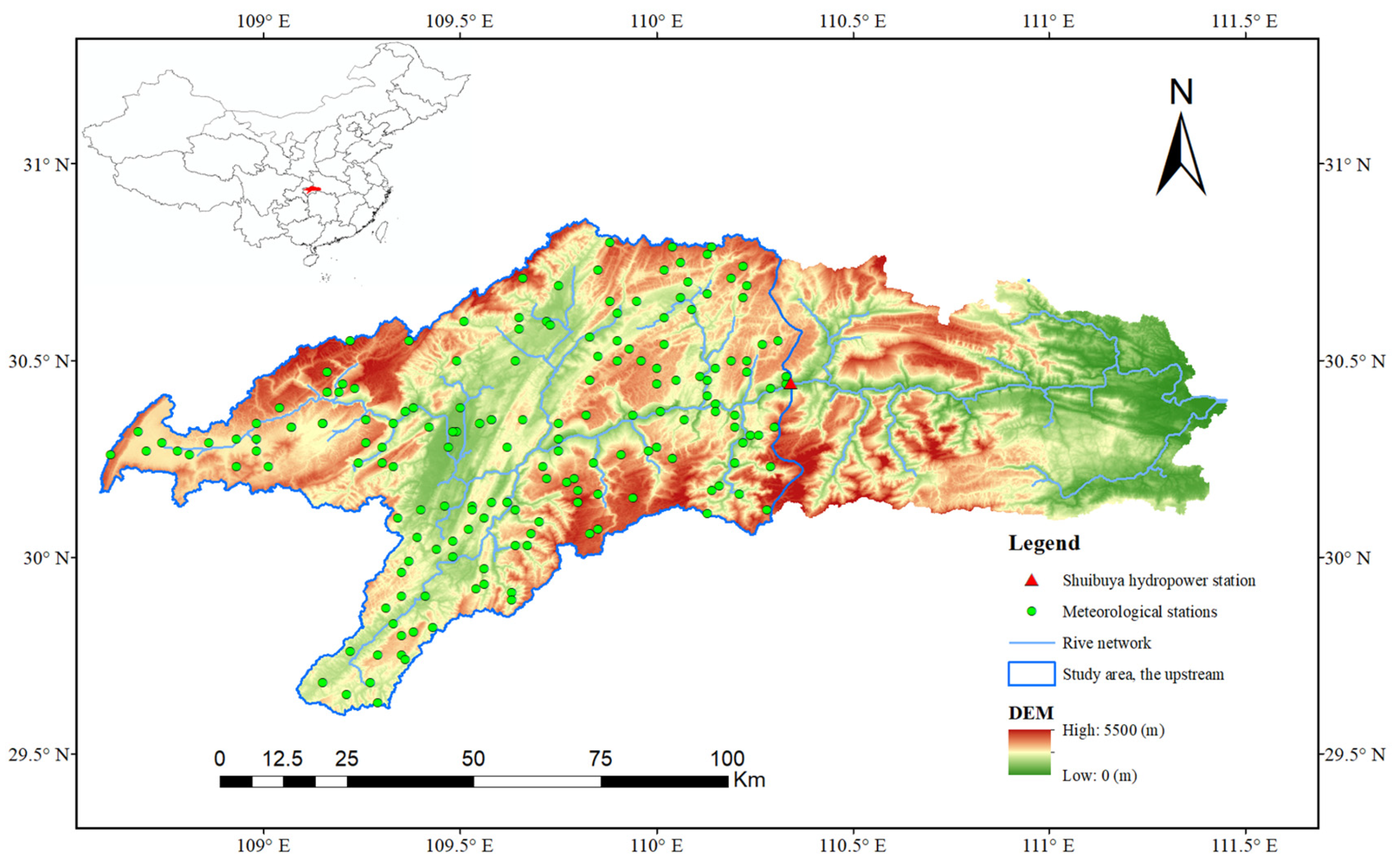
2. Study Area and Datasets

The Qingjiang River basin is located in the south-central region of China, specifically in southwestern Hubei Province (108°35′–111°35′ E, 22°33′–30°50′ N), as illustrated in Figure 1. It is a tributary of the upper Yangtze River, with a stream length of approximately 423 km. It drains a total area nearing 16,700 km², which is predominantly characterized by mountains and hills, accounting for 80% of its land cover. The elevation in the west is higher than that in the east. The basin experiences an average annual temperature of approximately 14 °C, and receives an average annual precipitation of approximately 1400 mm. The climatic influence of the humid subtropical monsoon is evident, with nearly 45% of the annual precipitation being received during the summer months (June–August). The rainstorms in summer are responsible for the basin’s seasonally variable flow regime, which contribute to around 40% of the annual streamflow. It is noteworthy to mention that human-induced activities, particularly dam constructions, affect the downstream regions of this basin. To reduce such influences and focus on more natural flow regimes, this study is centered on the upper Qingjiang River basin, which is relatively less affected by anthropogenic interventions. The outlet of this section is the Shuibuya hydropower station.

Table 1. The datasets used in this study.

Datasets	Sources	Ensemble Members (Perturbed)	Temporal/Spatial Resolution	Temporal Coverage
Observed meteorological data	175 meteorological stations	-	Daily/station	2014–2018 summer
Ensemble precipitation forecasts (EPFs)	CMA (China Meteorological Administration)	15	Seven lead days at six hours /0.5°	2014–2018 summer
	ECMWF (European Centre for Medium-Range Weather Forecasts)	50
	JMA (Japan Meteorological Administration)	26
	NCEP (National Centers for Environmental Prediction)	20
Observed streamflow	Shuibuya hydropower station	-	Daily/station	2014–2017 summer

presents a comprehensive list of datasets used in this study, including observed meteorological data and four EPFs collected during the summer periods of 2014–2018, as well as observed hydrological data collected during the summer periods of 2014–2017. The observed meteorological data, including air temperature, precipitation, and potential evaporation, were collated from 175 automatic meteorological stations distributed across the upper Qingjiang River basin. The basin-averaged values were derived through arithmetic mean calculations using these observations. The observed precipitation was used to assess and post-process the EPFs as a benchmark, as well as to calibrate the hydrological model together with the other observed meteorological data. The EPFs, used for precipitation and streamflow forecasts, were obtained from four renowned NWP centers, i.e., the CMA, ECMWF, JMA, and NCEP. The ensemble numbers for these EPFs are 15, 50, 26, and 20, respectively. The values of the EPFs collected every six hours were aggregated with daily metrics. All the gridded EPFs were then translated to basin-averaged values using the Thiessen polygon approach. Consistent with previous findings that precipitation forecasts lose their skill beyond seven days, this study incorporates forecasts only up to one week. Lastly, the observed hydrological data obtained from the Shuibuya hydropower station was used for hydrological model calibration and validation. Based on these datasets, this study post-processed EPFs from the summers of 2014–2018 and conducted hydrological modeling from the summers of 2014–2017.

3. Methodology

3.1. Post-Processing Methods

In this study, two state of art post-processing methods, a distribution-based method, BMA, and a generator-based method, GPP, were used to correct ensemble precipitation forecasts. They have been widely used in the domain of meteorology and hydrology [19,21,22,27].

First and foremost, the parametric PDF for the precipitation is defined, represented as $g$:

$$y|x_1,\dots ,x_M~g(y|x_1,\dots ,x_k)$$

(1)

where y is the precipitation variable and $x_1,\dots ,x_k$ corresponds to the ensemble precipitation forecasts comprising K members. Notably, the distribution of g for precipitation can be described as a mixed discrete/continuous model. This includes a nonzero probability of being zero and a continuous, skewed distribution for positive precipitation amounts. Sloughter, Raftery [15] proposed the mixed distribution model for precipitation as:

$$g(y|f_k)=P(y=0|f_k)·I(y=0)+P(y>0|f_k)·g_k(y|f_k)·I(y>0)$$

(2)

where $g(y|f_k)$ represents the probability distribution given the member forecast; $f_k$. I[…] equals one if its argument is true and zero otherwise; $P(y=0|f_k)$ and $g(y>0|f_k)$ represent the probabilities of non-precipitation and precipitation for a given forecast, $f_k$, respectively; and $g_k(y|f_k)$ represents a two-parameter gamma distribution.

The difference between the chosen post-processing methods lies in their approach to calibrating the precipitation PDF and their consequent generation of post-processed ensemble precipitation forecasts.

3.1.1. The BMA Method

For the distribution-based method, BMA, the precipitation PDF for a specific day or period is calibrated by fitting the forecast ensemble based on a historical dataset encompassing EPFs and observations, as follows:

$$P(y|f_1,\dots ,f_k)={\displaystyle \sum _{k=1}^K{W}_k{g}_k(y|f_k)}$$

(3)

where the weight, $W_k$, corresponds to the posterior probability of the selected ensemble member, k. This weight indicates the relative contribution of model k to the overall predictive skill during the training period. More details can be found in Raftery, Gneiting [14].

3.1.2. The GPP Method

For the generator-based method, GPP, calibration of the precipitation PDF is executed individually across distinct seasons or magnitudes and is aligned with relevant observations. The post-processed ensemble precipitation forecasts are then conditionally resampled from this calibrated PDF, using the forecast information in EPFs. More details can be found in Chen, Brissette [18].

Based on the EPFs and observed precipitation data from the summers from 2014–2018, this study adopted a cross-validation approach to optimize its post-processing methods. When forecasting for a specific year within this range, data from the remaining years served as the training dataset for calibration. For a comprehensive representation of the calibrated PDF, an ensemble size of 1000 was chosen. Two post-processing methods were, respectively, applied to each EPF; therefore, post-processed EPFs, i.e., BMA-EPFs and GPP-EPFs, were obtained. As an example, the term BMA-CMA refers to CMA forecasts that have undergone post-processing via the BMA method. The Matlab software was used for precipitation post-processing.

3.2. Hydrological Model

In this study, the Xin’anjiang (XAJ) model [28] was utilized for hydrological modelling because of its effective applications across the semi-humid and humid zones in China [21,29,30,31]. Within the framework of the lumped XAJ model, the basin is generalized into a soil box, encompassing an upper, lower, and deep soil layer. The computational mechanics of the XAJ consists of four modules: (1) the evaporation module, which utilizes the watershed saturation–excess runoff theory to ascertain evaporation rates. (2) The runoff yielding module, which uses the storage curve to calculate total runoff. This approach is based on the concept that runoff only forms when storage is replenished, indicating that runoff does not occur until soil moisture reaches its full capacity. (3) The runoff sources partitioning module, which uses a free water capacity distribution curve to divide the total runoff into three components: surface runoff, interflow, and groundwater runoff. (4) The runoff concentration module, in which the surface runoff is channeled using the unit hydrograph method, wherein both the interflow and groundwater runoff are directed using the linear reservoir approach. The XAJ model is configured with a total of fifteen parameters: four related to evaporation, two associated with runoff generation, and the remaining nine dedicated to runoff routing. These fifteen free parameters need to be calibrated by using the observed discharge data to effectively capture the hydrological characteristics of a specific basin [32]. An extensive exploration of these parameters can be found in Ren-Jun [28].

When the XAJ was built for the upper Qingjiang River basin, the summer periods of 2014–2016 and 2017 were used for calibration and validation, respectively. The basin-averaged inputs such as precipitation, temperature, and potential evaporation were used as inputs to yield an output of the basin outlet’s simulated discharge. The calibration was conducted using the SCE-UA algorithm [33] to refine the model parameter-sets according to the widely used objective function, the Nash–Sutcliffe coefficient (NSE) [34].

3.3. Verification Metrics

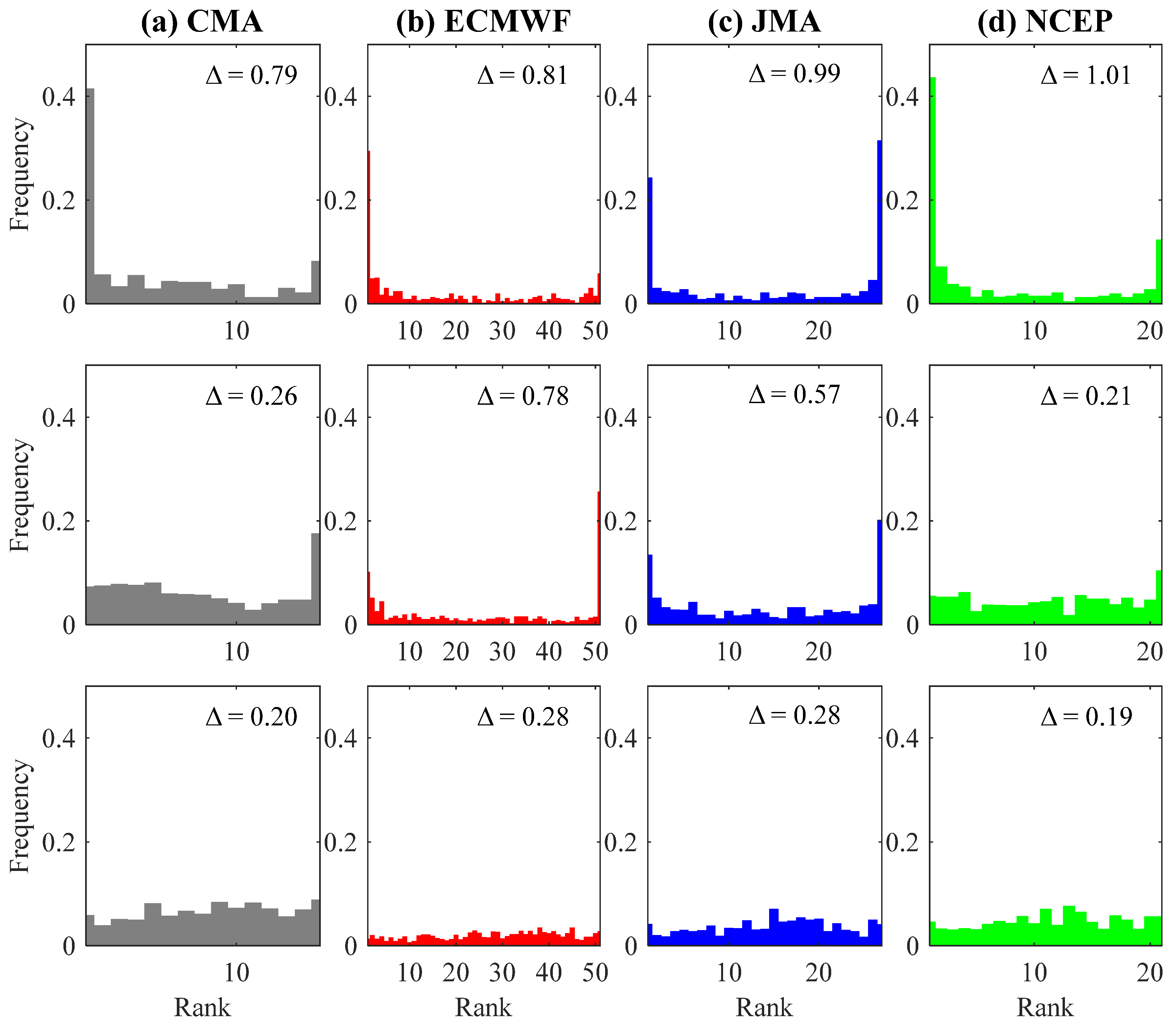
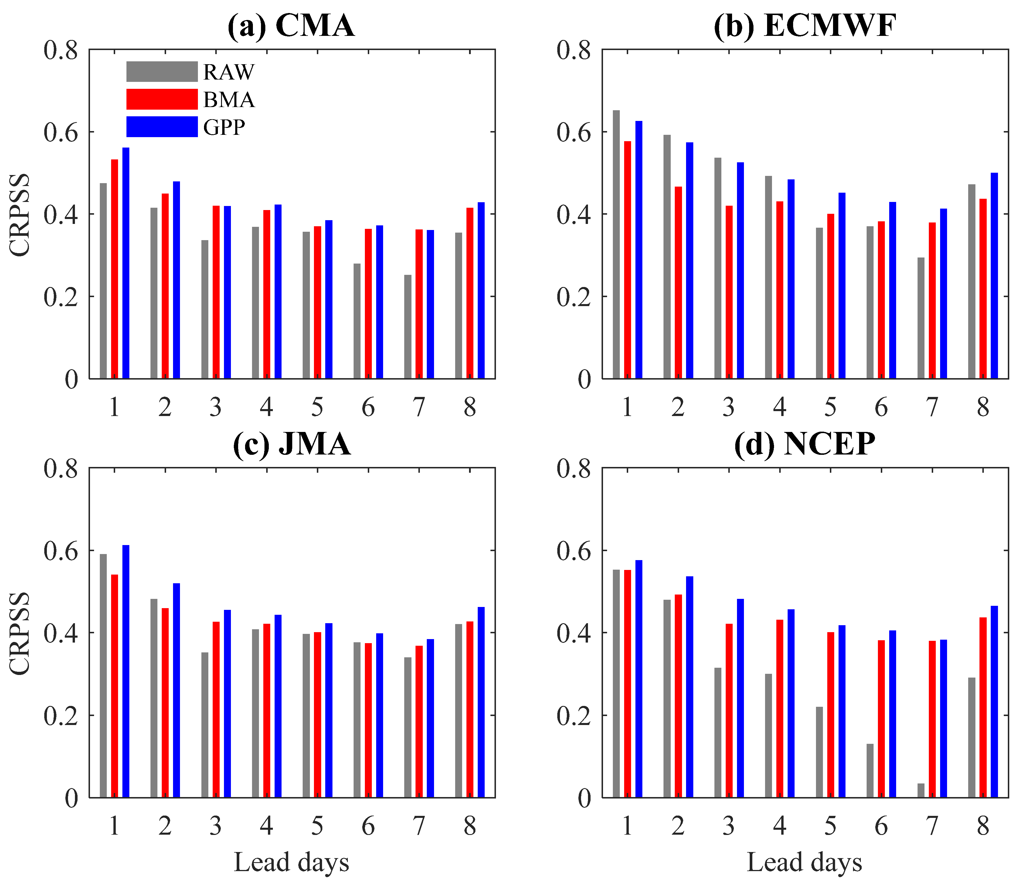
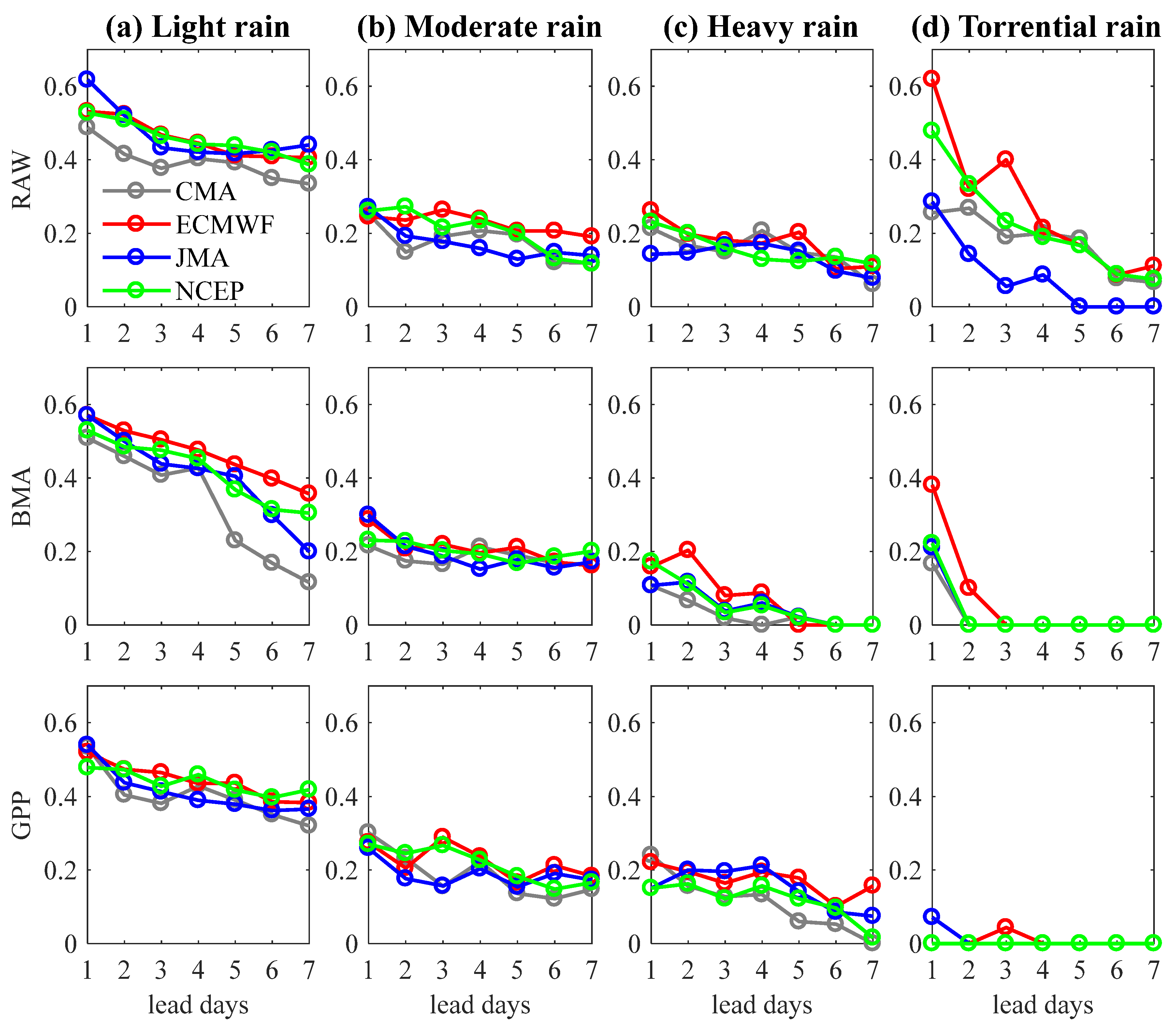
The evaluation of raw and post-processed EPFs was conducted using the basin-averaged value of observed precipitation during the 2014–2018 summer periods as a benchmark. As revealed in Brown, Demargne [35], relying solely on deterministic or probabilistic criteria is typically insufficient to assess EPF performance. Therefore, both deterministic and probabilistic metrics were adopted; the former was used to reflect the performance of ensemble mean forecasts and the latter was used to reflect the performance of ensemble forecasts. The deterministic metric used was the mean absolute error (MAE) [36], defined as:

$$MAE=\frac{1}{n}{\displaystyle \sum _{i=1}^n\left|F_i-O_i\right|}$$

(4)

where $F_i$ and $O_i$ are the EPFs and observed precipitation time series, respectively. $\overline{F_{}}$ and $\overline{O_{}}$ are the average of all daily values for EPFs and observed precipitation, respectively. $n$ is the length of daily time series. The MAE was used to assess the average absolute difference between the ensemble mean forecasts and the observations. MAE ranges from 0 to infinity, and a lower MAE signifies superior accuracy.

On the probabilistic front, the continuous ranked probability skill score (CRPSS) [37] and threat score (TS) [38] were adopted. The CRPSS is used to assess the performance of the ensemble spread of EPF over climatology, which is defined as the mean squared difference between the distribution of forecasts and corresponding distributions of observations:

$$CRPS={\displaystyle \underset{-\infty }{\overset{+\infty }{\int }}{\left(PF(x)-OF(x)\right)}^2}dx$$

(5)

$$CRPSS=1-\frac{CRPS}{CRP{S}^{*}}$$

(6)

where PF and OF are the cumulative distribution functions (CDFs) of the forecasts and observations, respectively. x represents the event to be analyzed. CRPS* is the value of the reference forecasts. The CRPSS ranges from negative infinity to 1, and a CRPSS value greater than 0 indicates skillful forecasts, with 1 being ideal.

The most widely used index, TS, was used to assess the performance of ensemble forecasts for four rainfall categories, i.e., light rain, moderate rain, heavy rain, and torrential rain.

Table 2. Category of valley area rainfall.

Category	24 h (mm)
Light rain	0.1–5.9
Moderate rain	6.0–14.9
Heavy rain	15–29.9
Torrential rain	>30

details the category of valley area rainfall [39]. TS is given by:

$$TS=\frac{N_A}{N_A+N_B+N_C}$$

(7)

Using the definitions of N_A, N_B, and N_C from the contingency table (

Table 3. Two-category contingency table.

Observations	Forecast
	Yes	No
Yes	NA	NC
No	NB	ND

), the TS can take values between 0 to 1; a TS value of 1 represents an ideal forecast, while 0 denotes no skill.

Additionally, the rank histogram, a renowned tool, was also used for ascertaining ensemble forecast reliability. As Heinrich [40] noted, a uniform rank histogram typifies a reliable forecast system, while deviations signify miscalibration. The associated reliability metric, Δ, quantifies departures from a flat histogram as:

$$\Delta ={\displaystyle \sum _{i=1}^{m+1}\left|F_i-\frac{1}{m+1}\right|}$$

(8)

where m is number of forecasting members, $\Delta$ ranges from 0 to 1, and a value of 0 symbolizes a flawless score and a balanced rank histogram.

For comprehensive insights on the aforementioned metrics, please refer to.

Turning to streamflow simulations and predictions, the NSE and relative error (RE) were used and given by:

$$NSE=1-\frac{{\displaystyle \sum _{i=1}^n(Q_i^{obs}-Q_i^{sim})}}{{\displaystyle \sum _{i=1}^n(Q_i^{obs}-\overline{Q_i^{obs}})}}$$

(9)

$$RE(\%)=\frac{{\displaystyle \sum _{i=1}^n(Q_i^{obs}-Q_i^{sim})}}{{\displaystyle \sum _{i=1}^n(Q_i^{obs})}}\times 100$$

(10)

where $Q_i^{obs}$ and $Q_i^{sim}$ are the daily streamflow for the observed and simulated time series, respectively. ${\overline{Q}}^{obs}$ is the average value of the observed streamflow. The NSE can take values between negative infinity and 1; a value of 1 indicates a perfect model and a value of 0 indicates that the model has the same predictive skill as the mean of the time-series. The RE can take values between negative infinity and 1; a smaller RE indicates a better performance.

4. Results

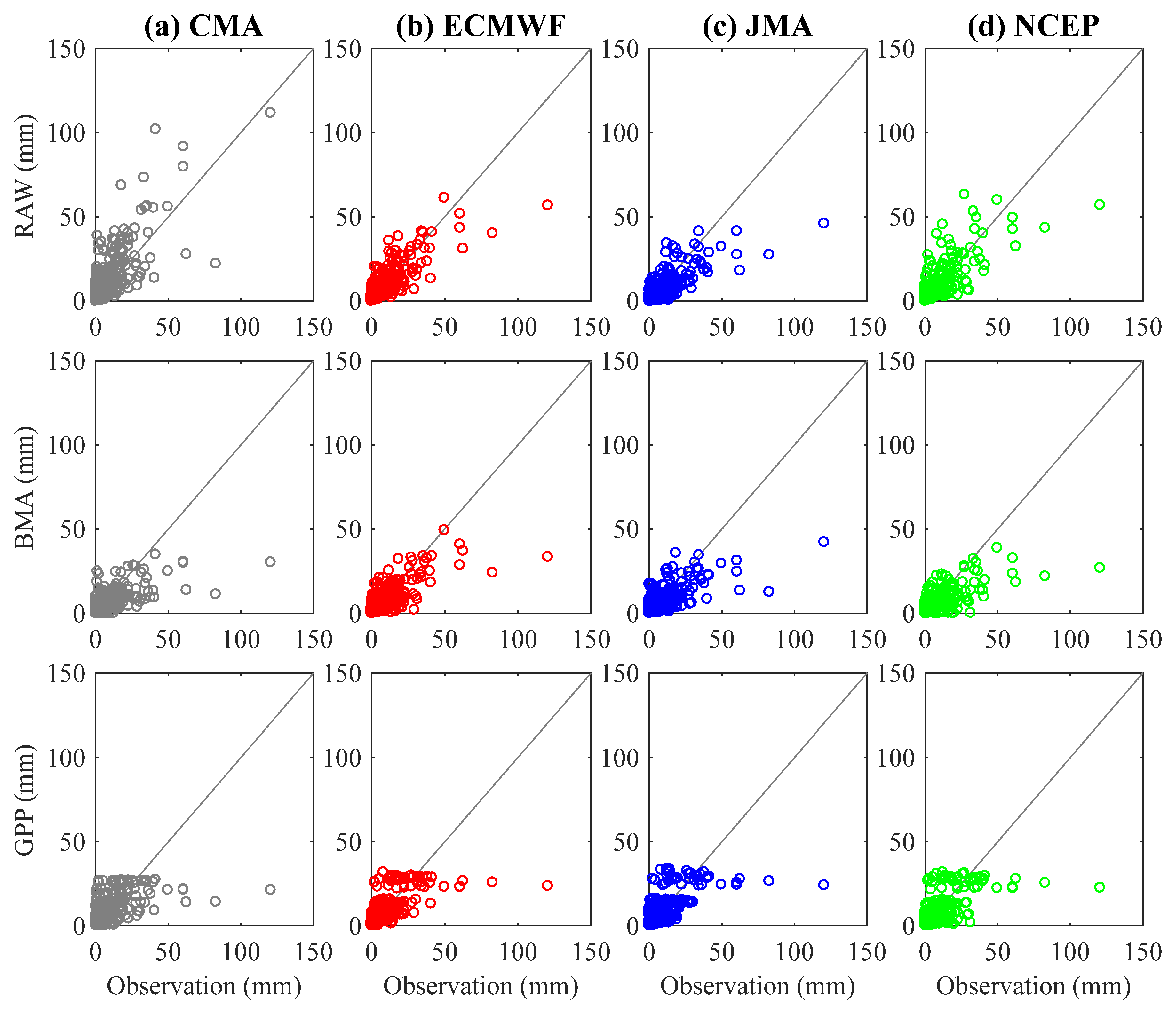
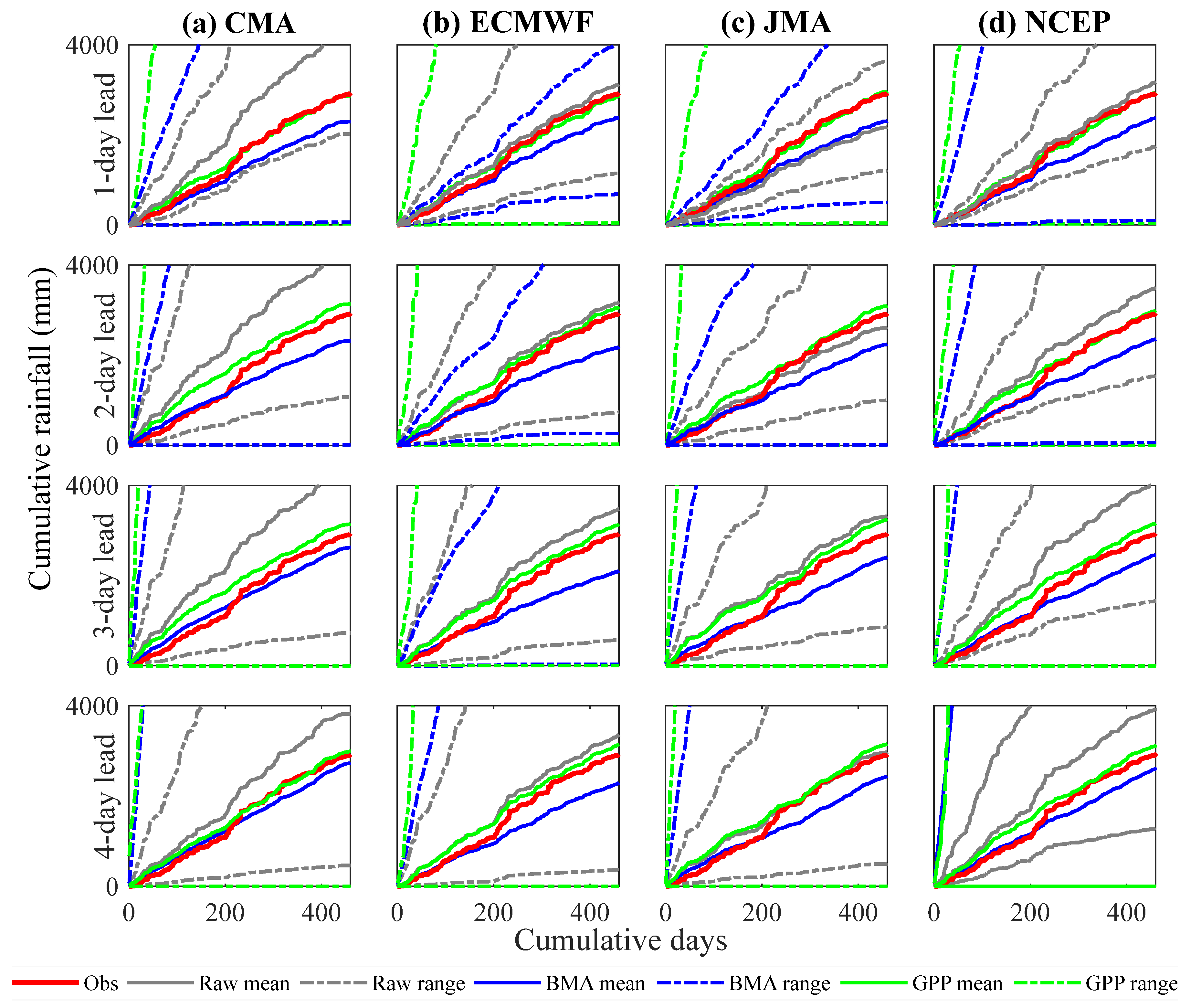
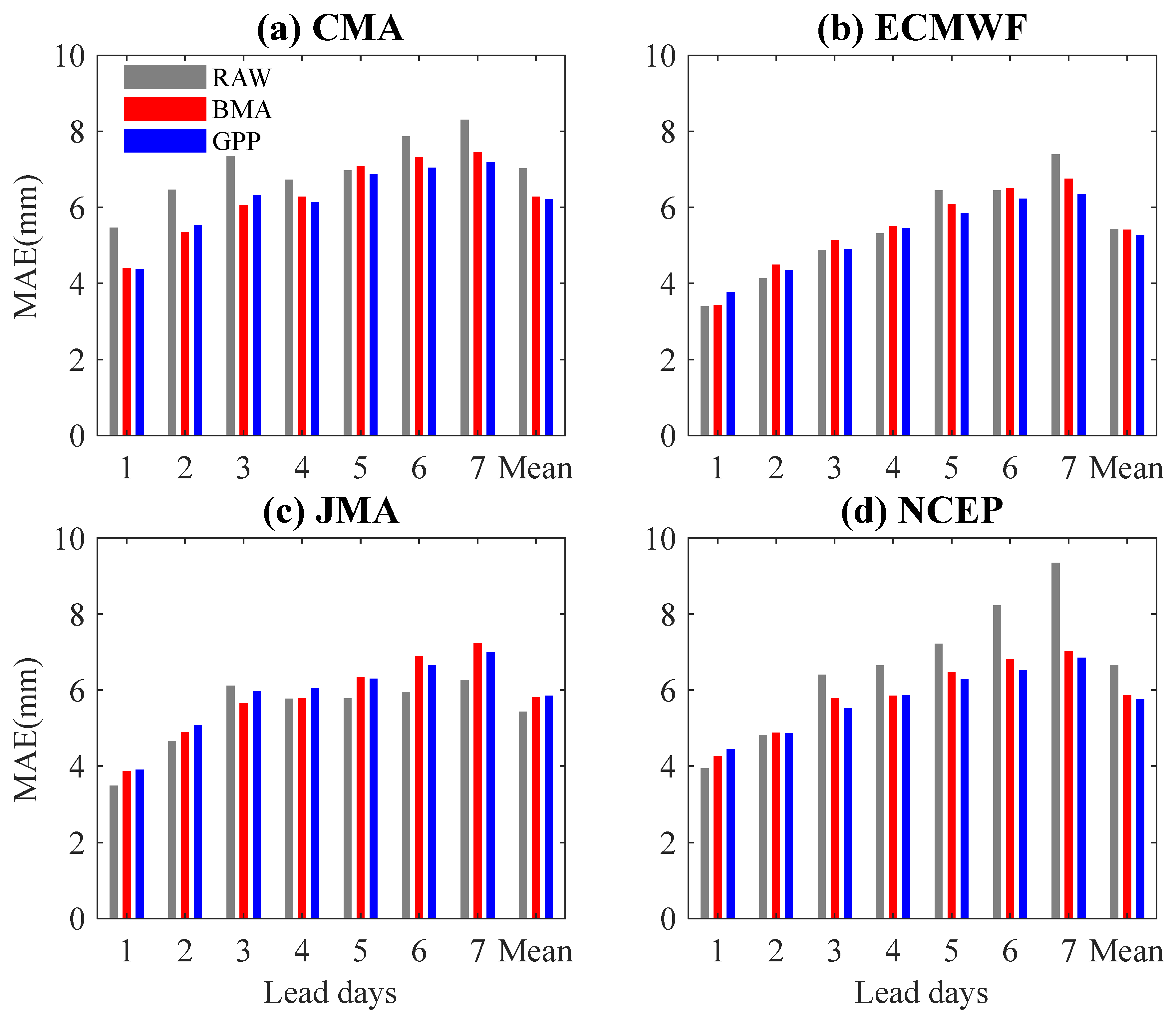
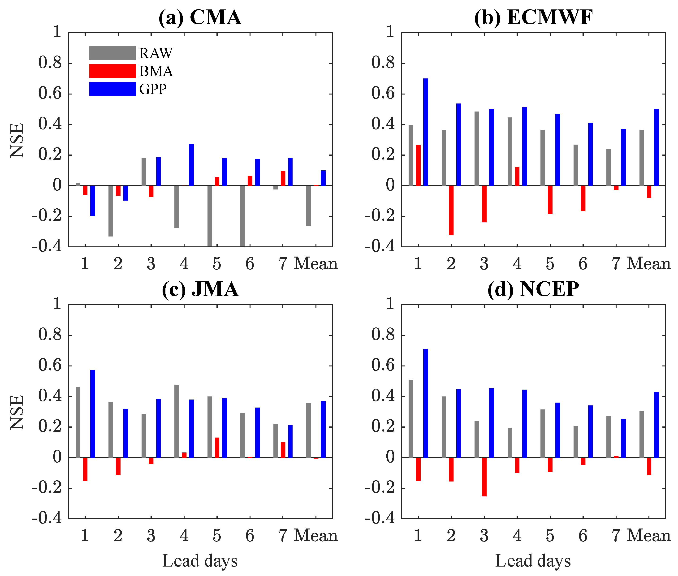
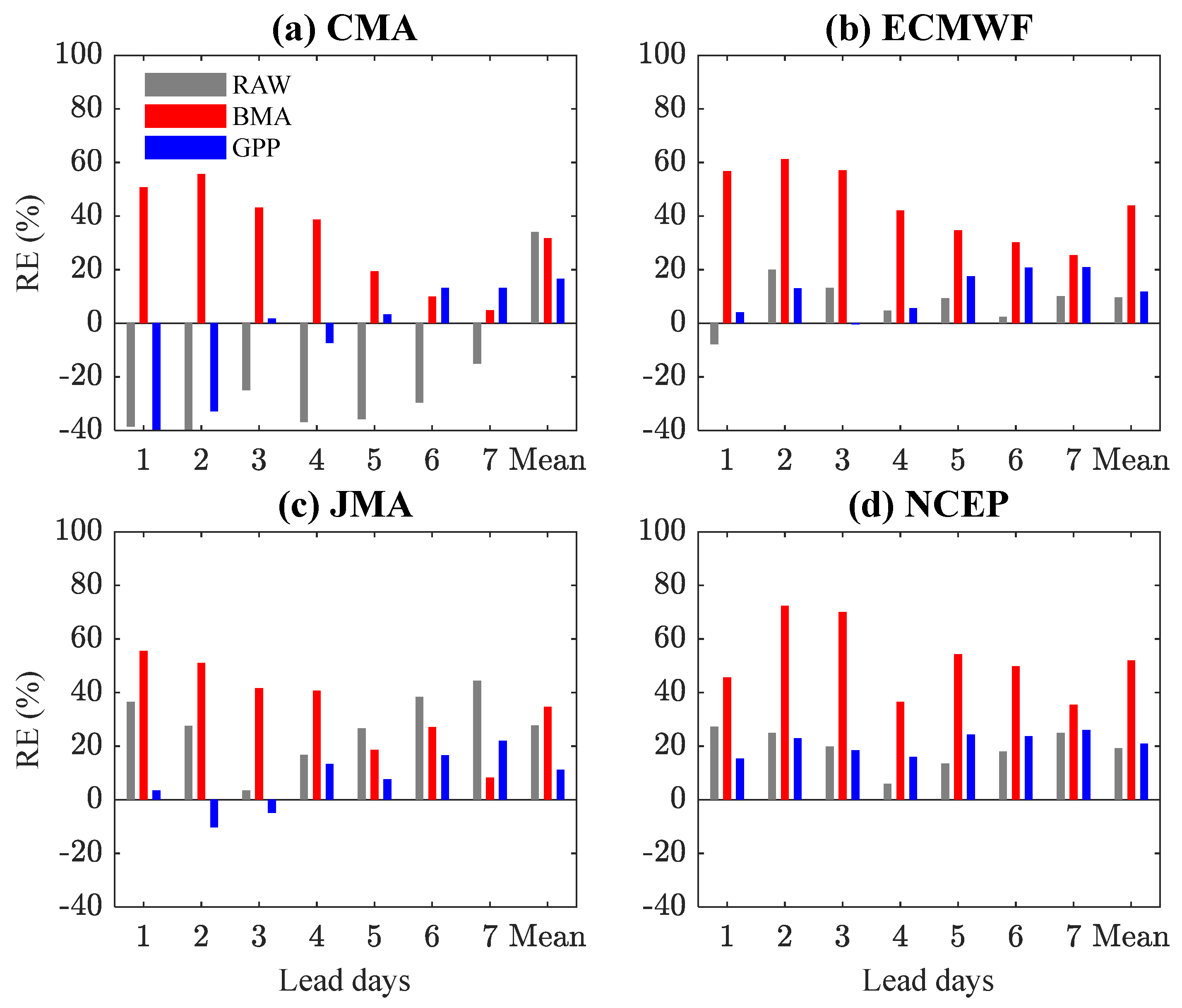
4.1. Post-Processing of the Ensemble Precipitation Forecasts

In this section, the raw and post-processed EPFs were compared with the observed precipitation using both deterministic and probabilistic metrics collected during the summers of 2014–2018 over the upper Qingjiang River basin. Figure 2 presents the scatter plots of observations and ensemble mean forecasts by the (a) CMA, (b) ECMWF, (c) JMA, and (d) NCEP at one lead day. The gray diagonal line is indicative of an ideal performance. Among the four raw EPFs (top row), even though the ECMWF and JMA show better performances, with scatters more clustered towards the grey diagonal, they generally underestimate precipitation at torrential rain rates (>30 mm). The CMA and NCEP show worse performances, especially for torrential rain rates, and are replete with large scatters, high false alarm rates, and large biases. After post-processing (middle and bottom rows), overestimation was reduced and underestimation of torrential rain rates could still be observed. The finding of the underestimation of torrential rain aligns with earlier studies [9,13]. The tendency to underestimate torrential rain poses challenges for hydrological forecasting, especially when predicting peak discharges and their timing, as underscored by Jha, Shrestha [41].

Figure 3 presents the time series of cumulative rainfall to evaluate the systematic error and the cover rate of ensemble forecasts. The range between the maximum member and the minimum member represents the dispersion. The post-processed EPFs (blue dash line, green dash line) show obviously larger dispersions than those of raw EPFs (gray dash line) and cover the raw EPFs well, except for the BMA-ECMWF (blue dash line in Column 2). Both the raw EPFs and EPFs post-processed by GPP (green dash line) show little variations in dispersion with the increasing lead days, while the dispersion of EPFs post-processed by BMA (blue dash line) increases with the increasing lead days. The ensemble means of GPP-EPFs (green solid line) are closer to the observed cumulative rainfall (red solid line) than those of raw (gray solid line) and BMA-EPFs (blue solid line). As the lead day increases, the cumulative rainfall error shifts from an overestimation to an underestimation, consistent with the findings of Yang, Yuan [26]. Generally, in terms of cumulative rainfall forecasting, the EPFs post-processed by GPP outperform the raw EPFs and those post-processed by BMA.

Figure 4 presents the performance of ensemble mean forecasts measured in MAE for the raw and post-processed (a) CMA, (b) ECMWF, (c) JMA, (d) NCEP data, at all seven lead days. The mean value of MAE is also presented. The MAE values of raw CMA, ECMWF, JMA, and NCEP data, respectively, range from 5.47~8.31, 3.40~7.41, 3.49~6.27, and 3.94~9.35 over 1-~7-lead days. This also shows better MAE performances by the ECMWF and JMA, with smaller values of mean MAE for all seven lead days than those of CMA and NCEP. The results show that by using post-processing methods, there are larger decreases in the mean MAE for CMA and NCEP than that of ECMWF. These methods are not desirable for the JMA, for which the MAE is even larger after post-processing. Specifically, by using the GPP method, the mean values of MAE decrease by about 0.81, 0.16, and 0.89 for the CMA, ECMWF, and NCEP, respectively. By using the BMA method, the mean values of MAE decrease by about 0.74, 0.02, and 0.79 for the CMA, ECMWF, and NCEP, respectively. Generally, in term of MAE, the ECMWF and JMA perform better than the CMA and NCEP. Two post-processing methods, especially GPP, can effectively decrease the MAE of the CMA and NCEP, which have poor raw performances.

Figure 5 presents the rank histograms for the raw and post-processed EPFs at one lead day. Heinrich [40] points out that it is useful to choose the same bin number when forecast systems with different ensemble sizes are compared. Therefore, for each post-processed EPF, the same bin number as that of the raw data is chosen from 1000 ensemble sizes to plot the histogram. There are 14, 50, 26, and 20 bins for the CMA, ECMWF, JMA, and NCEP, respectively. It can be seen that there are a large number of observations falling into the lowest and highest rank, forming a U-shaped rank histogram for raw EPFs (top row). The under-dispersive patterns of raw EPFs indicate underestimation of forecast uncertainty. Flatter histograms are obtained after post-processing (second and bottom rows), especially for the GPP EPFs (bottom row). Specifically, the reliability metric values decrease from 0.79 to 0.20, from 0.81 to 0.28, from 0.99 to 0.28, and from 1.01 to 0.19, for the CMA, ECMWF, JMA, and NCEP, respectively. In general, the post-processing methods, especially the GPP method, can effectively improve the under-dispersion of EPFs.

Figure 6 presents the probabilistic performance of ensemble forecasts measured in CRPSS for the raw and post-processed (a) CMA, (b) ECMWF, (c) JMA, and (d) NCEP data for all seven lead days. The mean value of CRPSS is also presented. The CRPSS values of the raw CMA, ECMWF, JMA, and NCEP data, respectively, range from 0.25~0.48, 0.30~0.65, 0.33~0.60, and 0.04~0.55 over 1-~7-lead days. This shows an overall decreasing trend with the increasing lead days. The mean values of CRPSS are 0.35, 0.47, 0.42, and 0.30 for the CMA, ECMWF, JMA, and NCEP, respectively. Among them, the ECMWF shows a better probabilistic performance, with a larger CRPSS value. In term of CRPSS, the probabilistic skills of EPFs are generally improved after post-processing. Specifically, the GPP method performs better than BMA method, with improvements of, on average, 0.07, 0.03, 0.04, and 0.17 for the ECMWF, JMA and NCEP, respectively.

Figure 7 presents the probabilistic performance of ensemble forecasts measured in TS for the raw and post-processed (a) CMA, (b) ECMWF, (c) JMA, (d) NCEP data across four categories. The figure shows a generally decreasing trend in TS with the increasing lead days for each rainfall category, especially for torrential rain. Generally, there is better TS performance for smaller precipitation categories. As for light rain, the ECMEF, JMA, and NCEP are comparable, showing good performances, with TS values above 0.4 for all seven lead days. The TS value of the CMA is relatively lower than those of other three. As for moderate rain and heavy rain, the four EPFs are comparable. The TS for torrential rain ranges largely among the different EPFs, and the ECMWF shows a relatively larger value. There is little improvement in TS by using both BMA (middle row) and GPP (bottom row) methods when compared to raw EPFs (top row). The improvement is relatively more effective for the CMA when forecasting light rainfall using GPP method, with increases from 0.32~0.48 to 0.33~0.53 at 1-~7-lead days, while EPFs give even worse performances when forecasting torrential rain after post-processing.

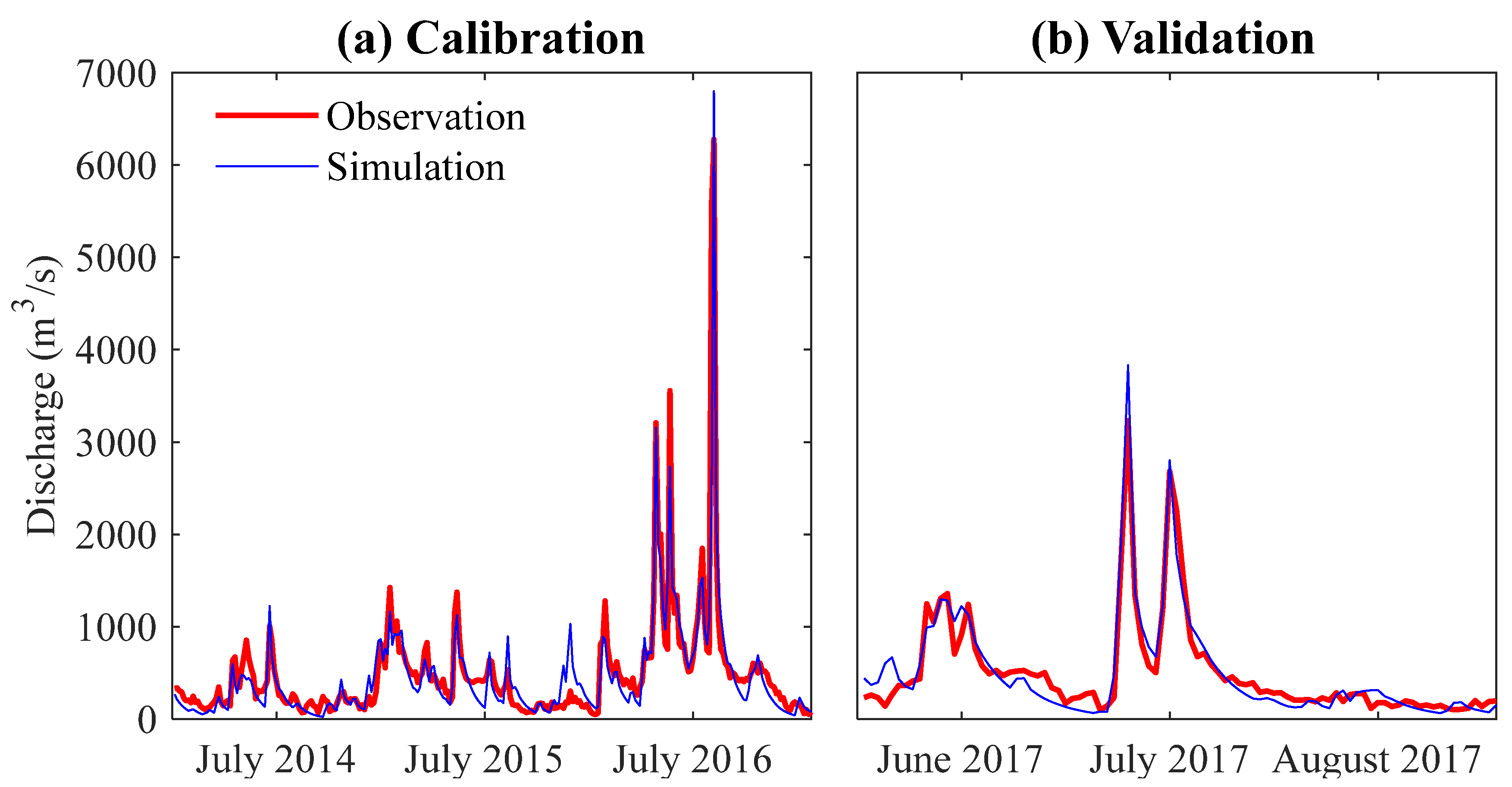
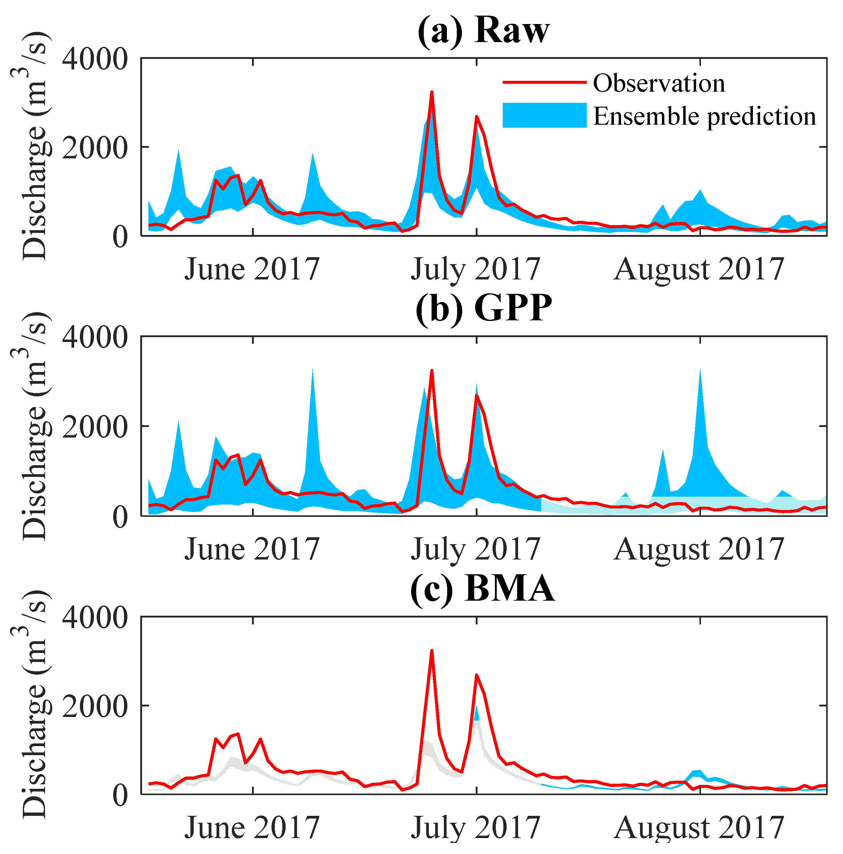
4.2. Application in Streamflow Prediction

In this section, the application of EPFs in streamflow prediction and the efficacy of BMA and GPP methods were evaluated. Firstly, the XAJ model was calibrated with observed streamflow using observed precipitation, temperature, and evaporation from the summers of 2014–2016 as inputs. This model was then validated for the summer of 2017. Subsequently, individual precipitation ensemble members of both raw and post-processed EPFs were applied to drive the calibrated XAJ model, generating streamflow ensembles. These were then used to derive the ensemble mean of streamflow prediction.

Figure 8 presents the time series of the simulated and observed streamflow during both calibration and validation periods. The NSE values are 0.91 and 0.89 for the calibration and validation periods, respectively, and the RE values are 9.3% and −2.6% for the calibration and validation periods, respectively. The XAJ shows a good applicability in terms of NSE and RE compared with earlier studies [27,30]. It also can be seen that both the peak and low flows are well captured by the simulated discharge. The results demonstrate that the XAJ model is accurately calibrated and thus can be used for streamflow prediction.

Figure 9 and Figure 10, respectively, present the NSE and RE for the ensemble means of streamflow simulated by the raw and post-processed (a) CMA, (b) ECMWF, (c) JMA, and (d) NCEP data for all seven lead days. The mean values of the NSE and absolute RE are also presented. The mean values of the NSE for the raw CMA, ECMWF, JMA, and NCEP data are, respectively, −0.26, 0.36, 0.35, and 0.30 for all seven lead days. According to previous studies [42,43], NSE = 0 is regularly used as a benchmark to distinguish “good” and “bad” models. Based on this provided benchmark, the CMA is unsuitable for predicting streamflow. In addition, Schaefli and Gupta [42] pointed out that reported NSE values can be properly interpreted while providing appropriate reference values. In this study, a skillful performance is set to be above 0.4, which is larger than that of the best model, i.e., the ECMWF. By using the GPP method, the mean values of NSE are overall improved for the four EPFs, among which the CMA shows the largest improvement, with an increase of 0.36. The mean values of the NSE for GPP-CMA, GPP-ECMWF, GPP-JMA, and GPP-NCEP are, respectively, 0.1, 0.5, 0.37, and 0.43 for all seven lead days. The NSE values of GPP-ECMWF are all above 0.4, and those of GPP-CMA are all below 0.4 for all seven lead days. The NSE values of GPP-ECMWF are above 0.4 at the first four lead days, and those of GPP-JMA are above 0.4 only at one lead day. The RE values of the raw CMA, ECMWF, JMA, and NCEP data, respectively, range from −58~−15%, −7.88~20%, 3.4~44%, and 5.89~27% over 1-~7-lead days. The CMA shows a general underestimation of streamflow, while the other three show general overestimations of streamflow. The mean value of absolute RE, respectively, decreases by 17%, and 16% for GPP-CMA and GPP-JMA. The decreases in absolute RE for GPP-ECMWF and GPP-NCEP are not significant. Using the BMA method, the NSE values generally decrease and the RE values generally increase for the four EPFs. This indicates that EPF post-processed by BMA leads to a worse skill in streamflow prediction. In addition, it shows a generally decreasing trend for NSE values and a generally increasing trend for RE values with the increasing lead days. In general, taking into account both the NSE and RE, the results show that the ECMWF is the most skillful model. It can add an additional lead time up to the seventh lead day after post-processing with the GPP method. Zhang, Chen [22] identified a ten lead day period in streamflow predictions using post-processed precipitation forecasts. The diminished performance of this study may be ascribed to the inherent challenges of estimating precipitation in the complex terrain of the mountain river basin.

The results above show that the ECMWF is more skillful in streamflow prediction among the four EPFs. Figure 11 further presents the hydrograph of ensemble streamflow driving using raw and post-processed ECMWF data at one lead day during the summer of 2017. The observed streamflow is also presented. The figure shows that the trend of observations is well captured by predictions both for the peak and low flows. The peak occurrence time predicted by raw ECMWF data closely matches the observations, while peak streamflow is considerably underestimated during July. The ECMWF ensemble underestimates the first peak event (9 July) and the second peak event (15 July) by about −16.51% and −6.57%, respectively. By using the GPP method, the prediction of GPP-ECMWF is improved in terms of generating the hydrograph. Specifically, GPP-ECMWF ensemble underestimates the first peak event (9 July) and the second peak event (15 July) by about −11.87% and −3.83%, respectively. Although the underestimation of peak streamflow was reduced, a certain degree of underestimation still could be observed. This is probably resulted from the underestimation of heavy rain rates (Figure 2). In addition, it can be seen that the ensemble prediction driven by GPP-ECMWF can better cover observations than that driven by raw ECMWF data. By using the BMA method, there is little improvement in predicting the ensemble mean streamflow compared with raw ECMWF data. The ensemble range cannot cover observed streamflow, with the maximum BMA-ECMWF ensemble member underestimating observations.

5. Discussion and Conclusions

EPFs play a pivotal role in extending forecast lead times and minimizing the uncertainties associated with precipitation predictions. When harnessed correctly, EPFs enhance both the reliability and accuracy of streamflow predictions by driving hydrological models. Nonetheless, given their inherent bias and under-dispersion, effective post-processing is imperative for corrections. In this study, four popular EPFs, i.e., the CMA, ECMWF, JMA, and NCEP, were post-processed by two state-of-the-art methods, i.e., the BMA and GPP methods, before their application to summer streamflow predictions using the XAJ model for a mountainous river basin. For a comprehensive evaluation, the deterministic metric MAE and the probabilistic CRPSS and TS metrics were utilized for precipitation forecast assessment. Streamflow prediction performance was analyzed using the NSE and RE metrics. Both precipitation forecasts and streamflow predictions were assessed before and after post-processing. Additionally, skillful forecast lead times of summer streamflow prediction restored by post-processing methods were also investigated.

In general, compared with the observed precipitation amount, the ensemble mean forecasts by the CMA, ECMWF, JMA, and NCEP exhibit biases, notably underestimating torrential rain. Liu, Sun [44] identified a consistent underestimation of heavy precipitation across China, with particular emphasis on the western and southern regions. This systematic underestimation can be attributed to factors such as resolution and the related convection parameterization. Furthermore, forecasts distinctly demonstrate under-dispersive tendencies, suggesting a marked underestimation of uncertainty in probabilistic precipitation forecasts. Of the EPFs assessed, the ECMWF and JMA outperform the NCEP and CMA in terms of precipitation ensemble mean forecasts, showing lower MAE values. The ECMWF performed better in precipitation ensemble forecasts with higher CRPSS values and performed better in both light rain and torrential rain forecasts with higher TS values. The superior performance of the ECMWF has been ascertained by plenty of studies [11,21,45]. In addition, the ECMWF’s prowess extends to streamflow predictions, which shows skill over 1-~4 lead days, with NSE values above 0.4 and absolute RE values below 20%. Despite this, there is underestimation of the observed peak discharge, underscoring the indispensability of post-processing EPFs to improve the application of precipitation forecasts to streamflow predictions.

The effectiveness of precipitation correction varies depending on the post-processing methods selected. In this study, both the GPP and BMA methods effectively countered the under-dispersion of EPFs and improved their deterministic performances as measured by the MAE. Specifically, the GPP method also showcased an improvement in probabilistic accuracy in terms of CRPSS, aligning with the findings of Li, Chen [27]. Regarding the TS, only minimal enhancements for the CMA at light rain rates were achieved using the GPP method. Post-processing torrential rain proves challenging due to its dual discrete–continuous nature and the notably non-normal distribution of its errors [12]. The advantage of GPP can be propagated to the performance of streamflow forecasts. After post-processing with the GPP method, the ECMWF ensemble mean can add additional lead times up to the seventh lead day, as indicated by its well behaved NSE and RE metrics. The underestimations of two peak flows at one lead day are reduced by about 4.64% and 2.74%, respectively. Conversely, while the BMA method’s contributions to precipitation forecast accuracy were marginal, this translated into limited advancements in streamflow prediction accuracy. This study underscores the significance of selecting a robust post-processing method for EPFs, whether for meteorological or hydrological applications.

Overall, this study underscores the potential benefits of EPFs for enhancing both precipitation forecasting and streamflow predictions when they are adeptly post-processed. Such methodologies could be extrapolated for application in other mountainous terrains. Nonetheless, the research is not devoid of constraints; likewise, the paucity of observational data from mountainous terrains and the uncertainties germinating from the deployment of a solitary hydrological model pose constraints. Additionally, the post-processing methods adopted in this study are applied to a single weather variable at a single location, neglecting the intersite and intervariable dependence structures of forecast variables [46]. It is well worth exploring further the potential advantages of integrating multisite and multivariable correlations during post-processing, which may amplify the precision of streamflow forecasts.

References

1. Roulin, E. Skill and relative economic value of medium-range hydrological ensemble predictions. Hydrol. Earth Syst. Sci. 2007, 11, 725–737. [Google Scholar] [CrossRef]
2. Sun, X.; Zhang, H.; Wang, J.; Shi, C.; Hua, D.; Li, J. Ensemble streamflow forecasting based on variational mode decomposition and long short term memory. Sci. Rep. 2022, 12, 518. [Google Scholar] [CrossRef]
3. Xu, Y.-P.; Tung, Y.-K. Decision-making in Water Management under Uncertainty. Water Resour. Manag. 2007, 22, 535–550. [Google Scholar] [CrossRef]
4. Troin, M.; Arsenault, R.; Wood, A.W.; Brissette, F.; Martel, J. Generating Ensemble Streamflow Forecasts: A Review of Methods and Approaches Over the Past 40 Years. Water Resour. Res. 2021, 57, e2020WR028392. [Google Scholar] [CrossRef]
5. Alfieri, L.; Pappenberger, F.; Wetterhall, F.; Haiden, T.; Richardson, D.; Salamon, P. Evaluation of ensemble streamflow predictions in Europe. J. Hydrol. 2014, 517, 913–922. [Google Scholar] [CrossRef]
6. Aminyavari, S.; Saghafian, B. Probabilistic streamflow forecast based on spatial post-processing of TIGGE precipitation forecasts. Stoch. Environ. Res. Risk Assess. 2019, 33, 1939–1950. [Google Scholar] [CrossRef]
7. Shukla, S.; Voisin, N.; Lettenmaier, D.P. Value of medium range weather forecasts in the improvement of seasonal hydrologic prediction skill. Hydrol. Earth Syst. Sci. 2012, 16, 2825–2838. [Google Scholar] [CrossRef]
8. Cloke, H.; Pappenberger, F. Ensemble flood forecasting: A review. J. Hydrol. 2009, 375, 613–626. [Google Scholar] [CrossRef]
9. Huang, L.; Luo, Y. Evaluation of quantitative precipitation forecasts by TIGGE ensembles for south China during the presummer rainy season. J. Geophys. Res. Atmos. 2017, 122, 8494–8516. [Google Scholar] [CrossRef]
10. Weidle, F.; Wang, Y.; Smet, G. On the Impact of the Choice of Global Ensemble in Forcing a Regional Ensemble System. Weather Forecast. 2016, 31, 515–530. [Google Scholar] [CrossRef]
11. Liu, L.; Gao, C.; Zhu, Q.; Xu, Y.-P. Evaluation of TIGGE Daily Accumulated Precipitation Forecasts over the Qu River Basin, China. J. Meteorol. Res. 2019, 33, 747–764. [Google Scholar] [CrossRef]
12. Scheuerer, M.; Hamill, T.M. Statistical Postprocessing of Ensemble Precipitation Forecasts by Fitting Censored, Shifted Gamma Distributions. Mon. Weather Rev. 2015, 143, 4578–4596. [Google Scholar] [CrossRef]
13. Dulière, V.; Zhang, Y.; Salathé, E.P. Extreme precipitation and temperature over the US Pacific Northwest: A comparison between observations, reanalysis data, and regional models. J. Clim. 2011, 24, 1950–1964. [Google Scholar] [CrossRef]
14. Raftery, A.E.; Gneiting, T.; Balabdaoui, F.; Polakowski, M. Using Bayesian Model Averaging to Calibrate Forecast Ensembles. Mon. Weather Rev. 2005, 133, 1155–1174. [Google Scholar] [CrossRef]
15. Sloughter, J.M.L.; Raftery, A.E.; Gneiting, T.; Fraley, C. Probabilistic Quantitative Precipitation Forecasting Using Bayesian Model Averaging. Mon. Weather Rev. 2007, 135, 3209–3220. [Google Scholar] [CrossRef]
16. Hamill, T.M.; Hagedorn, R.; Whitaker, J.S. Probabilistic Forecast Calibration Using ECMWF and GFS Ensemble Reforecasts. Part II: Precipitation. Mon. Weather Rev. 2008, 136, 2620–2632. [Google Scholar] [CrossRef]
17. Roulin, E.; Vannitsem, S. Postprocessing of ensemble precipitation predictions with extended logistic regression based on hindcasts. Mon. Weather Rev. 2012, 140, 874–888. [Google Scholar] [CrossRef]
18. Chen, J.; Brissette, F.P.; Li, Z. Postprocessing of Ensemble Weather Forecasts Using a Stochastic Weather Generator. Mon. Weather Rev. 2014, 142, 1106–1124. [Google Scholar] [CrossRef]
19. Schmeits, M.J.; Kok, K.J. A Comparison between Raw Ensemble Output, (Modified) Bayesian Model Averaging, and Extended Logistic Regression Using ECMWF Ensemble Precipitation Reforecasts. Mon. Weather Rev. 2010, 138, 4199–4211. [Google Scholar] [CrossRef]
20. Williams, R.M.; Ferro, C.A.T.; Kwasniok, F. A comparison of ensemble post-processing methods for extreme events. Q. J. R. Meteorol. Soc. 2013, 140, 1112–1120. [Google Scholar] [CrossRef]
21. Qu, B.; Zhang, X.; Pappenberger, F.; Zhang, T.; Fang, Y. Multi-Model Grand Ensemble Hydrologic Forecasting in the Fu River Basin Using Bayesian Model Averaging. Water 2017, 9, 74. [Google Scholar] [CrossRef]
22. Zhang, J.; Chen, J.; Li, X.; Chen, H.; Xie, P.; Li, W. Combining Postprocessed Ensemble Weather Forecasts and Multiple Hydrological Models for Ensemble Streamflow Predictions. J. Hydrol. Eng. 2020, 25, 04019060. [Google Scholar] [CrossRef]
23. Vetter, T.; Reinhardt, J.; Flörke, M.; Van Griensven, A.; Hattermann, F.; Huang, S.; Koch, H.; Pechlivanidis, I.G.; Plötner, S.; Seidou, O.; et al. Evaluation of sources of uncertainty in projected hydrological changes under climate change in 12 large-scale river basins. Clim. Chang. 2017, 141, 419–433. [Google Scholar] [CrossRef]
24. Mascaro, G.; Vivoni, E.R.; Deidda, R. Implications of Ensemble Quantitative Precipitation Forecast Errors on Distributed Streamflow Forecasting. J. Hydrometeorol. 2010, 11, 69–86. [Google Scholar] [CrossRef]
25. Anderson, M.L.; Chen, Z.-Q.; Kavvas, M.L.; Feldman, A. Coupling HEC-HMS with Atmospheric Models for Prediction of Watershed Runoff. J. Hydrol. Eng. 2002, 7, 312–318. [Google Scholar] [CrossRef]
26. Yang, C.; Yuan, H.; Su, X. Bias correction of ensemble precipitation forecasts in the improvement of summer streamflow prediction skill. J. Hydrol. 2020, 588, 124955. [Google Scholar] [CrossRef]
27. Li, X.-Q.; Chen, J.; Xu, C.-Y.; Li, L.; Chen, H. Performance of Post-Processed Methods in Hydrological Predictions Evaluated by Deterministic and Probabilistic Criteria. Water Resour. Manag. 2019, 33, 3289–3302. [Google Scholar] [CrossRef]
28. Ren-Jun, Z. The Xinanjiang model applied in China. J. Hydrol. 1992, 135, 371–381. [Google Scholar] [CrossRef]
29. Xiang, Y.; Peng, T.; Gao, Q.; Shen, T.; Qi, H. Evaluation of TIGGE Precipitation Forecast and Its Applicability in Streamflow Predictions over a Mountain River Basin, China. Water 2022, 14, 2432. [Google Scholar] [CrossRef]
30. Shu, Z.; Zhang, J.; Jin, J.; Wang, L.; Wang, G.; Wang, J.; Sun, Z.; Liu, J.; Liu, Y.; He, R.; et al. Evaluation and Application of Quantitative Precipitation Forecast Products for Mainland China Based on TIGGE Multimodel Data. J. Hydrometeorol. 2021, 22, 1199–1219. [Google Scholar] [CrossRef]
31. Peng, T.; Wang, J.; Tang, Z.; Ding, H. Analysis for calculating critical area rainfall on different time scales in small and medium catchment based on hydrological simulation. Torrential Rain Disasters 2017, 36, 365–372. [Google Scholar] [CrossRef]
32. Shi, P.; Chen, C.; Srinivasan, R.; Zhang, X.; Cai, T.; Fang, X.; Qu, S.; Chen, X.; Li, Q. Evaluating the SWAT Model for Hydrological Modeling in the Xixian Watershed and a Comparison with the XAJ Model. Water Resour. Manag. 2011, 25, 2595–2612. [Google Scholar] [CrossRef]
33. Duan, Q.Y.; Gupta, V.K.; Sorooshian, S. Shuffled complex evolution approach for effective and efficient global minimization. J. Optim. Theory Appl. 1993, 76, 501–521. [Google Scholar] [CrossRef]
34. Nash, J.E.; Sutcliffe, J.V. River flow forecasting through conceptual models part I—A discussion of principles. J. Hydrol. 1970, 10, 282–290. [Google Scholar] [CrossRef]
35. Brown, J.D.; Demargne, J.; Seo, D.-J.; Liu, Y. The Ensemble Verification System (EVS): A software tool for verifying ensemble forecasts of hydrometeorological and hydrologic variables at discrete locations. Environ. Model. Softw. 2010, 25, 854–872. [Google Scholar] [CrossRef]
36. Hong, J.-S. Evaluation of the High-Resolution Model Forecasts over the Taiwan Area during GIMEX. Weather Forecast. 2003, 18, 836–846. [Google Scholar] [CrossRef]
37. Ma, F.; Ye, A.; Deng, X.; Zhou, Z.; Liu, X.; Duan, Q.; Xu, J.; Miao, C.; Di, Z.; Gong, W. Evaluating the skill of NMME seasonal precipitation ensemble predictions for 17 hydroclimatic regions in continental China. Int. J. Clim. 2015, 36, 132–144. [Google Scholar] [CrossRef]
38. Mesinger, F. Bias Adjusted Precipitation Threat Scores. Adv. Geosci. 2008, 16, 137–142. [Google Scholar] [CrossRef]
39. GB/T 20486-2006; Category of Valley Area Rainfall. Standardization Administration of China: Beijing, China, 2006. Available online: https://www.chinesestandard.net/ (accessed on 25 October 2023).
40. Heinrich, C. On the number of bins in a rank histogram. Q. J. R. Meteorol. Soc. 2021, 147, 544–556. [Google Scholar] [CrossRef]
41. Jha, S.K.; Shrestha, D.L.; Stadnyk, T.A.; Coulibaly, P. Evaluation of ensemble precipitation forecasts generated through post-processing in a Canadian catchment. Hydrol. Earth Syst. Sci. 2018, 22, 1957–1969. [Google Scholar] [CrossRef]
42. Schaefli, B.; Gupta, H.V. Do Nash values have value? Hydrol. Processes 2007, 21, 2075–2080. [Google Scholar] [CrossRef]
43. Moriasi, D.N.; Arnold, J.G.; van Liew, M.W.; Bingner, R.L.; Harmel, R.D.; Veith, T.L. Model evaluation guidelines for systematic quantification of accuracy in watershed simulations. Trans. ASABE 2007, 50, 885–900. [Google Scholar] [CrossRef]
44. Liu, C.; Sun, J.; Yang, X.; Jin, S.; Fu, S. Evaluation of ECMWF Precipitation Predictions in China during 2015–2018. Weather Forecast. 2021, 36, 1043–1060. [Google Scholar] [CrossRef]
45. Tao, Y.; Duan, Q.; Ye, A.; Gong, W.; Di, Z.; Xiao, M.; Hsu, K. An evaluation of post-processed TIGGE multimodel ensemble precipitation forecast in the Huai river basin. J. Hydrol. 2014, 519, 2890–2905. [Google Scholar] [CrossRef]
46. Chen, J.; Li, X.; Xu, C.-Y.; Zhang, X.J.; Xiong, L.; Guo, Q. Postprocessing Ensemble Weather Forecasts for Introducing Multisite and Multivariable Correlations Using Rank Shuffle and Copula Theory. Mon. Weather Rev. 2022, 150, 551–565. [Google Scholar] [CrossRef]
Figure 1. The Qingjiang river basin.
Atmosphere 14 01645 g001
Figure 2. Scatter plots of observed and forecasted area rainfall from the (a) CMA, (b) ECMWF, (c) JMA, and (d) NCEP at one lead day during the summers of 2014–2018. Lines 1–3 represent the raw, BMA, and GPP data, respectively.
Atmosphere 14 01645 g002
Figure 3. Time series of cumulative rainfall forecasts (mm) by the (a) CMA, (b) ECMWF, (c) JMA, and (d) NCEP during the summers of 2014–2018. Observations are also presented. Lines 1–4 represent 1-~4 lead days, respectively.
Atmosphere 14 01645 g003
Figure 4. Mean absolute error (MAE) for the raw and post-processed ensemble mean forecasts by the (a) CMA, (b) ECMWF, (c) JMA, and (d) NCEP at 1-~7 lead days. The mean value of MAE for all seven lead days are also presented.
Atmosphere 14 01645 g004
Figure 5. Rank histogram for the raw and post-processed ensemble forecasts by the (a) CMA (14 members), (b) ECMWF (50 members), (c) JMA (26 members), (d) NCEP (20 members) at one lead day. Lines 1–3 represent the raw, BMA, and GPP data, respectively.
Atmosphere 14 01645 g005
Figure 6. CRPSS for the raw and post-processed ensemble forecasts by the (a) CMA, (b) ECMWF, (c) JMA, and (d) NCEP at 1-~7 lead days. The mean value of CRPSS for all seven lead days is also presented.
Atmosphere 14 01645 g006
Figure 7. TS of the raw and post-processed CMA, ECMWF, JMA, and NCEP data at 1-~7 lead days for precipitation in four categories, i.e., (a) light rain, (b) moderate rain, (c) heavy rain, and (d) torrential rain. Lines 1–3 represent the raw, BMA, and GPP data, respectively.
Atmosphere 14 01645 g007
Figure 8. Time series of simulated discharge based on XAJ model during calibration (2014–2016 summer) and validation (2017 summer) periods, compared with observed streamflow.
Atmosphere 14 01645 g008
Figure 9. NSE for the ensemble mean of streamflow simulated by the raw and post-processed EPFs (CMA, ECMWF, JMA, and NCEP) at 1-~7 lead days. The mean value of NSE for all seven lead days is also presented.
Atmosphere 14 01645 g009
Figure 10. RE for the ensemble mean of streamflow simulated by the raw and post-processed EPFs (CMA, ECMWF, JMA, NCEP) at 1-~7 lead days during the summer of 2017. The mean value of the absolute RE for all seven lead days is also presented.
Atmosphere 14 01645 g010
Figure 11. Hydrograph of ensemble streamflow driving using raw and post-processed ECMWF data at one lead day during the summer of 2017 compared with observed hydrograph.
Atmosphere 14 01645 g011