
Impact of AIS Data Thinning on Ship Air Pollutant Emissions Inventories


1
China Waterborne Transport Research Institute, Beijing 100088, China
2
Shanghai Key Laboratory of Atmospheric Particle Pollution and Prevention (LAP3), National Observations and Research Station for Wetland Ecosystems of the Yangtze Estuary, Department of Environmental Science and Engineering, Fudan University, Shanghai 200433, China
*
Author to whom correspondence should be addressed.
Atmosphere 2022, 13(7), 1135; https://doi.org/10.3390/atmos13071135
Submission received: 25 May 2022
/
Revised: 6 July 2022
/
Accepted: 16 July 2022
/
Published: 18 July 2022
(This article belongs to the Special Issue Atmospheric Shipping Emissions and Their Environmental Impacts)
Abstract
:This article examines the impact of automatic identification system (AIS) data thinning on ship emissions inventory results. AIS data thinning is theoretically proven to lead to a smaller result for a ship’s air pollutant emissions inventory. The AIS dynamic data of six sampled ships for 1 day and for 1 year were thinned at 1 min, 3 min, 10 min, 30 min, and 1 h time intervals, and then CO2, NOX, CH, PM, SO2, and other air pollutant emissions were estimated both with and without AIS data thinning in the different time intervals. The results show that AIS data thinning affects the air pollutant emissions inventory results of the ships, and the impact is greater as the thinning interval increases. When the thinning interval is less than 10 min, the impact is less than 10%, but the impact increases to about 10–15% at a 30 min interval and about 15–20% at a 60 min interval. The impacts of thinning on the emissions of ships with acutely fluctuating speeds are more significant because the constantly changing speed is the main reason why data thinning affects the ship emissions inventory. Therefore, these data suggest that the AIS data can be thinned at intervals of 5 or 10 min when establishing a coastal or national ship air pollutant emissions inventory, the AIS data should be thinned at intervals of less than 3 min when establishing the air pollutant emissions inventory of inland river ships, and data thinning is not recommended when establishing a port or smaller-scale ship air pollutant emissions inventory.
1. Introduction
Ship air pollution has attracted a great deal of attention at home and abroad [1,2]. For example, studies have shown that ship emissions of SOx and NOX account for 39% and 28% of Denmark’s total emissions, respectively, and for 10% to 31% of the emissions from European countries such as the Netherlands, Sweden, Norway, the United Kingdom, France, Italy, Belgium, Finland, and Germany [3]. In recent years, the Chinese government and academia have also attached great importance to the control of air pollution from ships. According to the bulletin of the second national survey of pollution sources in China, the SO2, NOX, and PM emissions of ships operating in China’s waters are 42.08 × 10⁴ t, 102.48 × 10⁴ t, and 8.44 × 10⁴ t, accounting for 100%, 9.6%, and 3.3%, respectively, of the total emissions of the corresponding pollutants from all mobile sources [4]. On November 30, 2018, the Ministry of Transport issued the implementation plan of the ship air pollutant emission control area to strengthen the control of ship pollution emissions.
Emission inventory is the basis for quantifying the emission of air pollutants from ships and studying the formation, mechanism and effective control of compound pollution. Much academic research has focused on ship air pollution emission inventory in recent years [5], and the methodologies can be divided into the bottom-up dynamic method and the top-down fuel method. The top-down ship emissions inventory performed for the Emission Database for Global Atmospheric Research, EDGAR [6,7] was constructed from major global shipping routes and traffic intensities. Alternatively, the bottom-up method focuses on relatively precise shipping routes, and the emissions are estimated based on vessel activity. Compared to the top-down method, the bottom-up method has better spatial and temporal resolution. Using AIS data, the establishment of a ship emissions inventory has undergone a revolutionary change. Jalkanen et al. [8] established the first ship emissions inventory based on AIS data from the Baltic Sea. Goldsworthy et al. [1] built a ship emissions model system based on AIS data and used it to estimate the ship emissions inventory for the seas surrounding Australia. In 2002, ENTEC used the bottom-up method to establish the European ship air pollution emissions inventory based on ship operating conditions (from a navigation database) [9]. The work on ship emissions inventories in China has focused on the ports of Shanghai, Shenzhen, and Hong Kong. Yang et al. [10] estimated an emission inventory for marine ships in the Shanghai Port in 2003 using annual activity rates multiplied by emission factors. Fu et al. [11] calculated the total amount of air pollutant emissions in the Shanghai Port, and spatially gridded it onto the routes defined by AIS activity data with a month’s worth of spatial information to make full use of the AIS data. Li et al. [12] roughly estimated the SO2 emissions in the Shenzhen Port and ship emissions in Hong Kong. Ng et al. [13] established a ship emissions inventory in Hong Kong based on AIS data, and ship emissions inventories in Tianjin, Xiamen, and other ports were established successively [14,15,16]. In recent years, high-spatial resolution ship emissions inventories have been used to assess the impacts of ship emissions on air quality [17,18,19,20].
The earlier research was mainly based on the fuel method [21], whereas the dynamic method based on AIS has become the mainstream method with the ongoing development of ship dynamic monitoring technology [22,23]. AIS is a new type of navigation aid system that is applied to maritime safety and communication between ships and either shores or other ships, which can automatically exchange important information, such as the position, speed, course, name, and call sign of the ship. By using AIS data and the working mechanism of a ship’s engine to establish the emission inventory, it is possible to calculate the real-time pollutant emissions of a single ship. Compared to the fuel method, the dynamic method based on AIS has higher accuracy, so it can accurately analyze the pollutant emissions of a single ship at different times, and it is more adaptable for air pollution analyses with high temporal and spatial resolution and for determining the developmental trends of air pollution control [24]. According to the ITU-RM.1371-4 recommendation issued by the International Telecommunication Union, the intervals between static messages and dynamic messages sent by AIS equipment are different. Generally, the AIS-equipped ships send static messages every 6 min. When the data are calibrated or under other special circumstances, the static messages will be sent immediately as required. The interval for sending AIS dynamic messages depends on ship speed and heading. When the ship is anchored or moored and the speed is less than 3 knots, the interval for sending dynamic messages is 3 min. However, when the navigation speed is 0–14 knots, 14–23 knots, or greater than 23 knots (with changing course), the interval for sending dynamic messages is 10 s (10/3 s), 6 s (2 s), or 2 s (2 s), respectively.
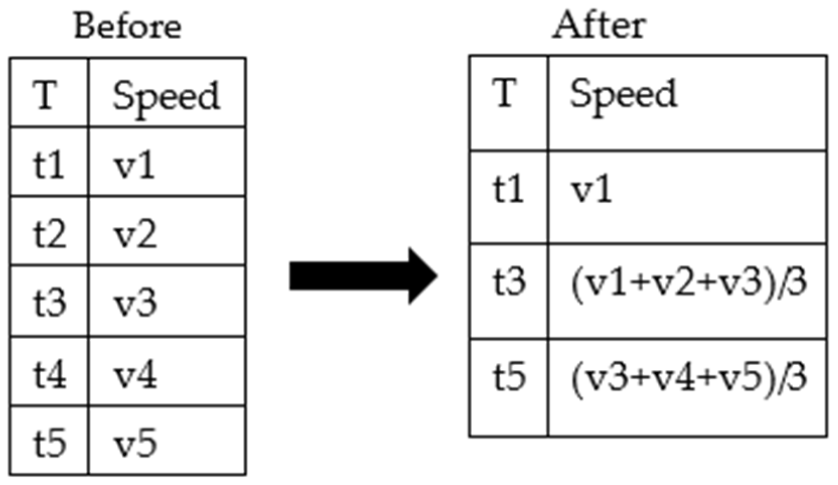
The AIS messages received by an AIS data receiving station are from all ships. There are high requirements for computing equipment and software because of the large amount of data, so AIS data are typically thinned in practical research [25]. AIS dynamic messages contain the navigation time, latitude, longitude, heading, speed, and other information about the ship. Data thinning is the process of reducing the dimensionality of latitude, longitude, and speed according to the time interval, which directly changes the ships’ navigation track and speed and further affects the results of the emissions inventory.
If the ship is sailing at a constant speed, data thinning has no effect on the ship’s speed. However, ships often do not travel at a uniform speed. The greater the time interval between messages, the greater the difference in the ship speed between the sending points of the AIS messages. In addition, this is also related to the shape of the channel. The greater the thinning interval of a curved channel, the greater the fluctuations in the speed. Therefore, AIS data thinning has a greater impact on inland navigation ships than coastal navigation ships. However, there are few reports on the extent of the impact from thinning.
In order to study the influence of AIS data thinning on the inventory, we first analyzed the impact of AIS data thinning on the results of the ships’ air pollutant emissions inventory theoretically. We then randomly selected the AIS dynamic data of six ships on a certain day in 2019, thinned the data in different time intervals, and estimated the changes in the CO2, NOX, CH, PM, SO2, and other air pollutant emissions of the sampled ships with and without AIS data thinning. This process allowed us to analyze the impact of the thinning of AIS data on the emissions inventory among six ships representing different patterns of movement.
2. Data
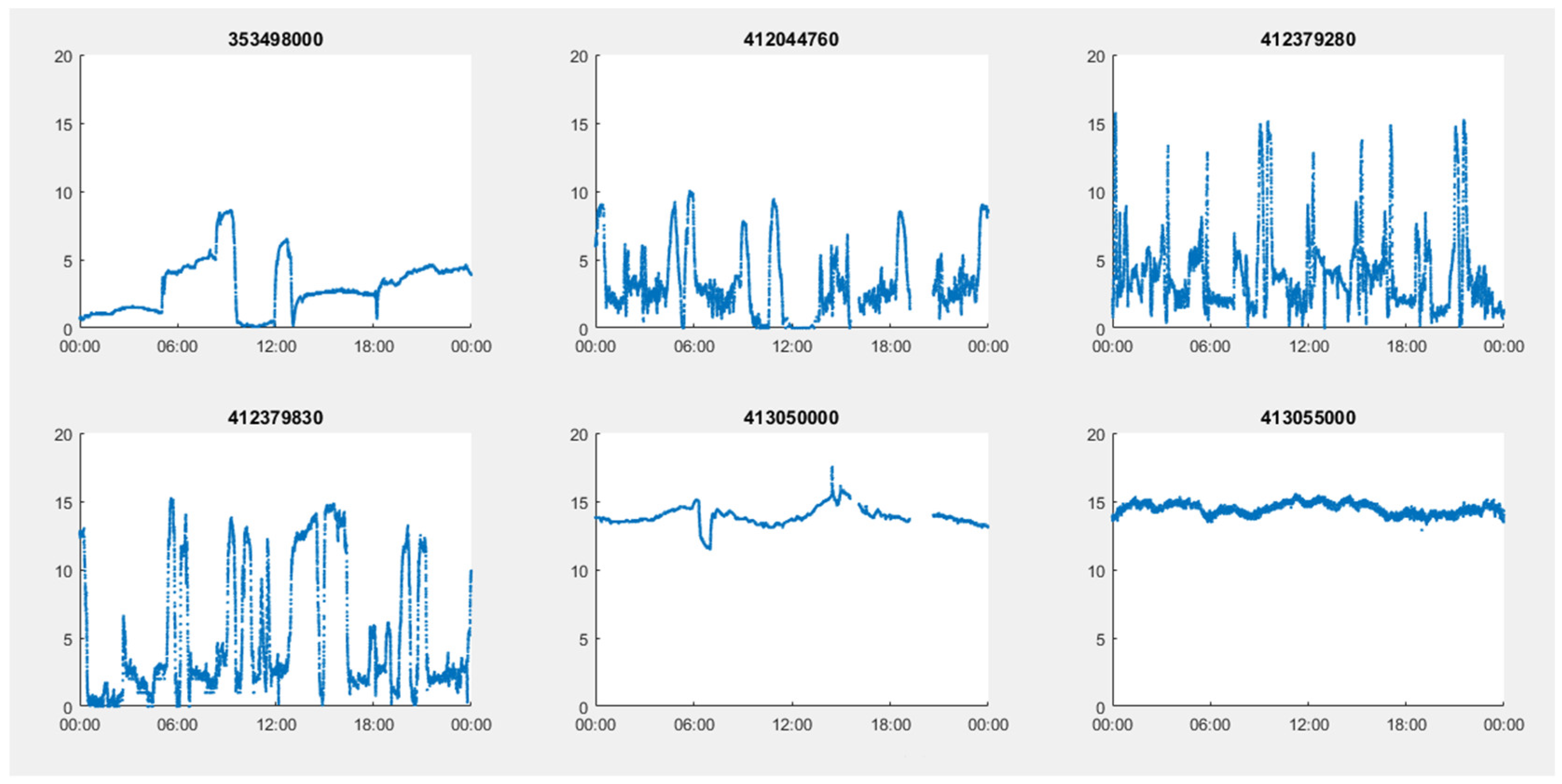
The AIS data of six ships (Table 1) for one day and for one year were randomly selected from all of the ships sailing in Chinese waters in 2019. All of the information required for the inventory, such as main engine power, rated speed, etc., was obtained by querying the ship registration database (Table 1). According to the AIS data for the selected day, the set of six ships includes two cruising ships (Ship 5 and Ship 6 in Table 1), two in-and-out port ships (Ship 3 and Ship 4 in Table 1), and two maneuvering ships (i.e., ships with significant speed changes and anchoring behavior, Ship 1 and Ship 2 in Table 1). Among the sampled ships, the fluctuating speed of in-and-out port ships is the largest, followed by maneuvering ships and cruising ships (Figure 1). The track chart of the six ships in 2019 was drawn according to the AIS data (Figure 2).
3. Methodology
3.1. Data Thinning
The thinning of AIS data can reduce the amount of data, speed up the calculations, and facilitate follow-up analysis and research, such as spatial and temporal analyses of the emissions. Despite these advantages, the impact of thinning has not been studied in detail. AIS data contains time information, and the thinning of AIS data increases the period between two adjacent AIS messages and cuts down the amount of data. Figure 3 shows the principle of data thinning.
3.2. Theoretical Analysis
The air pollutant emissions inventories of ships based on AIS data employ the STEAM (ship traffic exhaust assessment model) model proposed by Jalkanen [26].
where represent the pollutant emissions of the main engine, auxiliary engine, and auxiliary boiler, respectively.
where is the installed power of the main engine of a ship, measured in kW. is the load factor of the main engine, which reflects the ratio of its actual output power to the installed maximum power. is the low multiplier of load adjustment of the main engine to account for the fact that the main engine increases distinctly when its load rate is lower than 20%. represents the operating time of the main engine, measured in h. is the emission factor of the main engine, measured in g/kWh.
where represents the actual activity speed of the ship, which is the speed over water considering the influences of the environment, measured in knots, and is the design maximum speed of the ship, measured in knots.
AIS data thinning only affects the speed of a ship, and the speed affects the pollutant emissions of the main engine by changing its load factor. The emissions inventory of the main engine can be calculated as:
where is the design maximum speed of the ship, measured in knots, and , which is a constant for a sailing ship (i.e., when the main engine load is greater than 20%).
If the AIS data are thinned at the time interval of t, then the time interval and speed between adjacent messages before thinning are recorded as , respectively, where i = 0, 1, 2, …, n. When is approximately equal, the emissions with and without thinning are, respectively:
The details of the proof that are described in the Supplementary Materials (Supplementary Materials, Chapter S1). Therefore, theoretically the thinning process of AIS data will reduce the resulting ship air pollutant emission inventory.
3.3. Verification
The AIS dynamic data of the six sampled ships for one day and for one year were thinned at the time intervals of 1 min, 3 min, 10 min, 30 min, and 1 h. The extraction rules are: (i) the coordinates of the route track take the longitude and latitude of the middle point of the ship’s navigation track within the time intervals of 1 min, 3 min, 10 min, 30 min, and 1 h (and if the number of messages is even, then take the longitude and latitude of the first point in the middle); and (ii) the speed is the average of the actual ship speed at all points within each time period. The times in the first and the final messages will be the time after thinning.
For the steps in the calculation, firstly, the emissions of CO2, NOX, CH, PM, SO2, and other air pollutants from the six sampled ships for one day without thinning were estimated using Formulas (1)–(3). Secondly, the emissions of CO2, NOX, CH, PM, and SO2 for one day with thinning at each time interval were estimated. Each ship has various navigation states in a year. So, the emissions of CO2, NOX, CH, PM, SO2, and other air pollutants from the six sampled ships for one year without thinning and within the time intervals of 1 min, 3 min, 10 min, 30 min, and 1 h were estimated using the same method. Finally, the air pollutant emissions of the sampled ships in one day and one year with and without data thinning were compared and analyzed to illustrate the impact of data thinning on the air pollutant emissions inventories (Table 2 and Table 3). The verification results can be summarized by five main points.
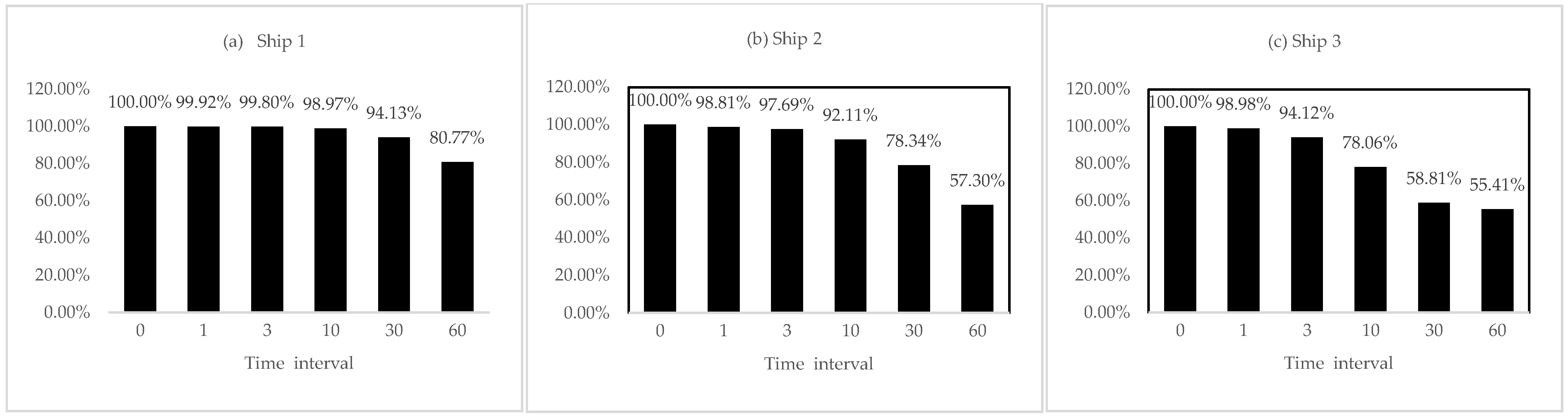
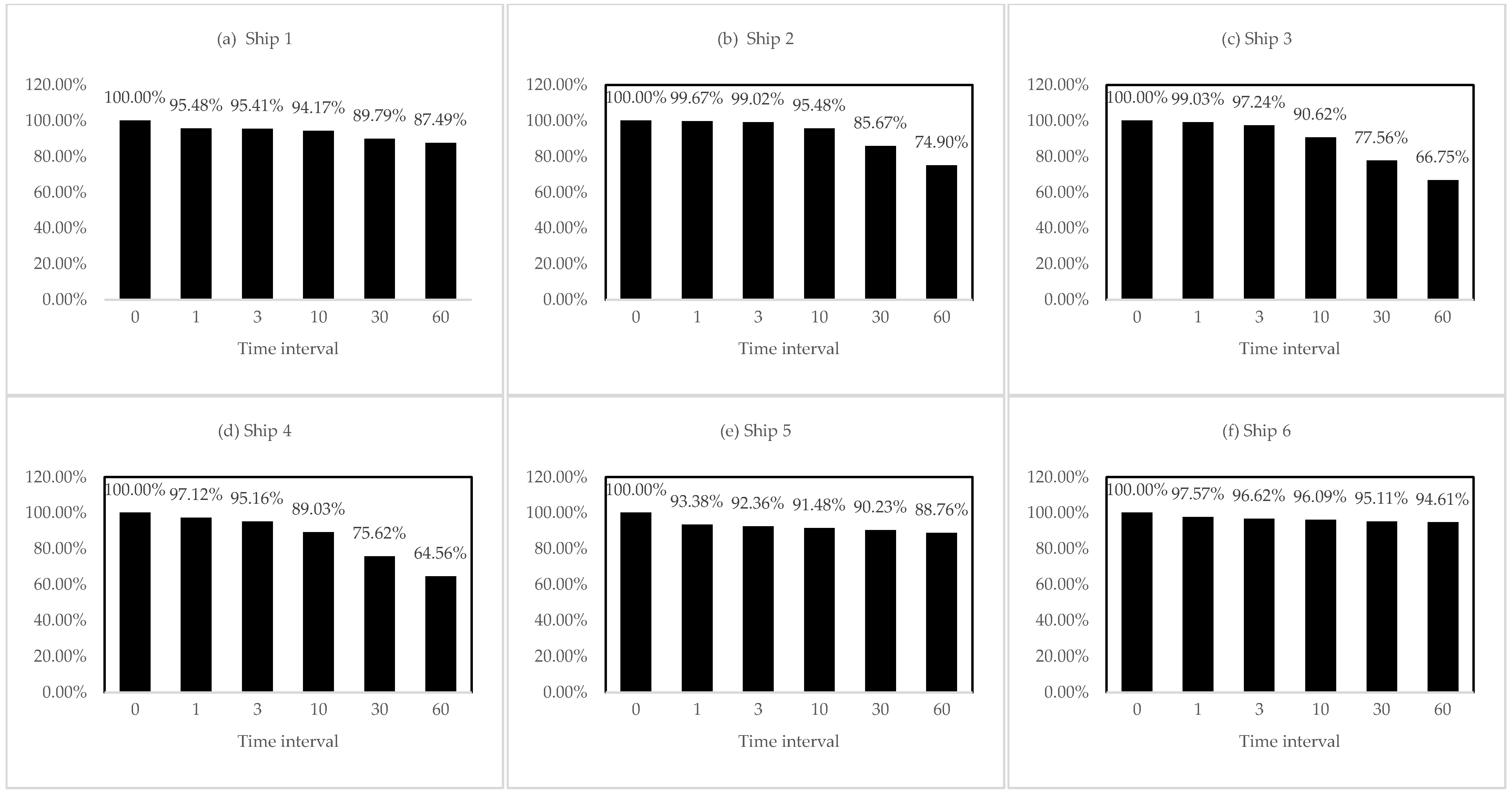
(1) The thinning of AIS data affects the results of a ship’s air pollutant emissions inventory, and the impact is greater, with an increase in the thinning interval (Figure 4 and Figure 5, and Figures S1–S5 in Supplementary Materials). Taking sample Ship 2 as an example, the emissions of CO2, CO, CH, NOX, PM10, and SO2 without thinning are 2.7308 t, 0.0048 t, 0.0022 t, 0.0555 t, 0.0016 t, and 0.0084 t, respectively. With thinning at a 3 min interval, CO2, CO, CH, NOX, PM10, and SO2 are reduced by 2.31%, 2.08%, 4.55%, 2.34%, 0.001%, and 2.38%, respectively; with thinning at a 10 min interval, they are reduced by 7.89%, 6.25%, 9.09%, 7.93%, 6.25%, and 8.33%, respectively; and with thinning at a 60 min interval, they are reduced by 42.7%, 41.67%, 40.91%, 42.88%, 43.75% and 42.86%, respectively.
(2) The thinning of AIS data has a more significant impact on the pollutant emissions of ships with acutely fluctuating speeds. After the data are thinned, the order of the reduction of air pollutant emissions from ships is: in-and-out port ships > maneuvering ships > cruise ships (see Figure 4 and Figures S1–S5 in Supplementary Materials).
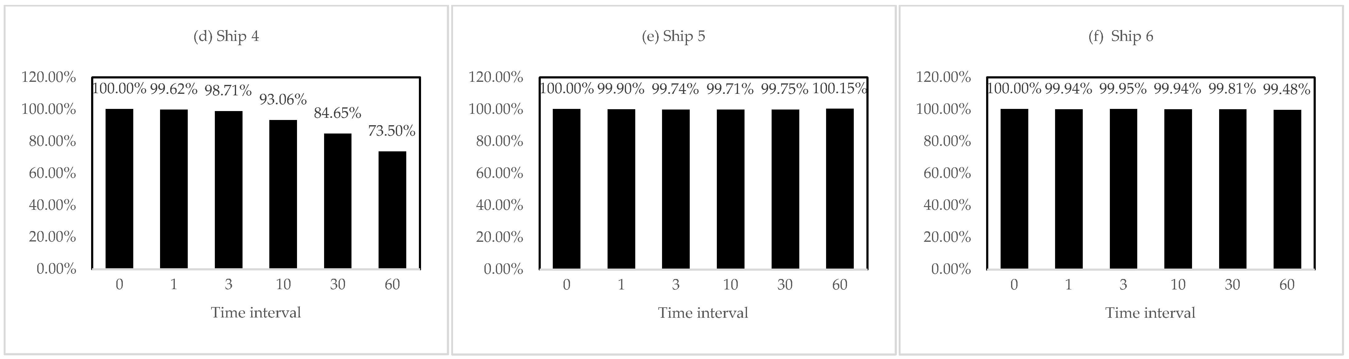
(3) When the thinning interval is less than 3 min, it has little impact on the emissions inventory, and the impacts of intervals greater than 3 min increase with an increasing time interval. When the thinning interval is more than 10 min, it has a significant impact on the annual emissions inventories (see Figure 5 and Figures S6–S10 in SI).
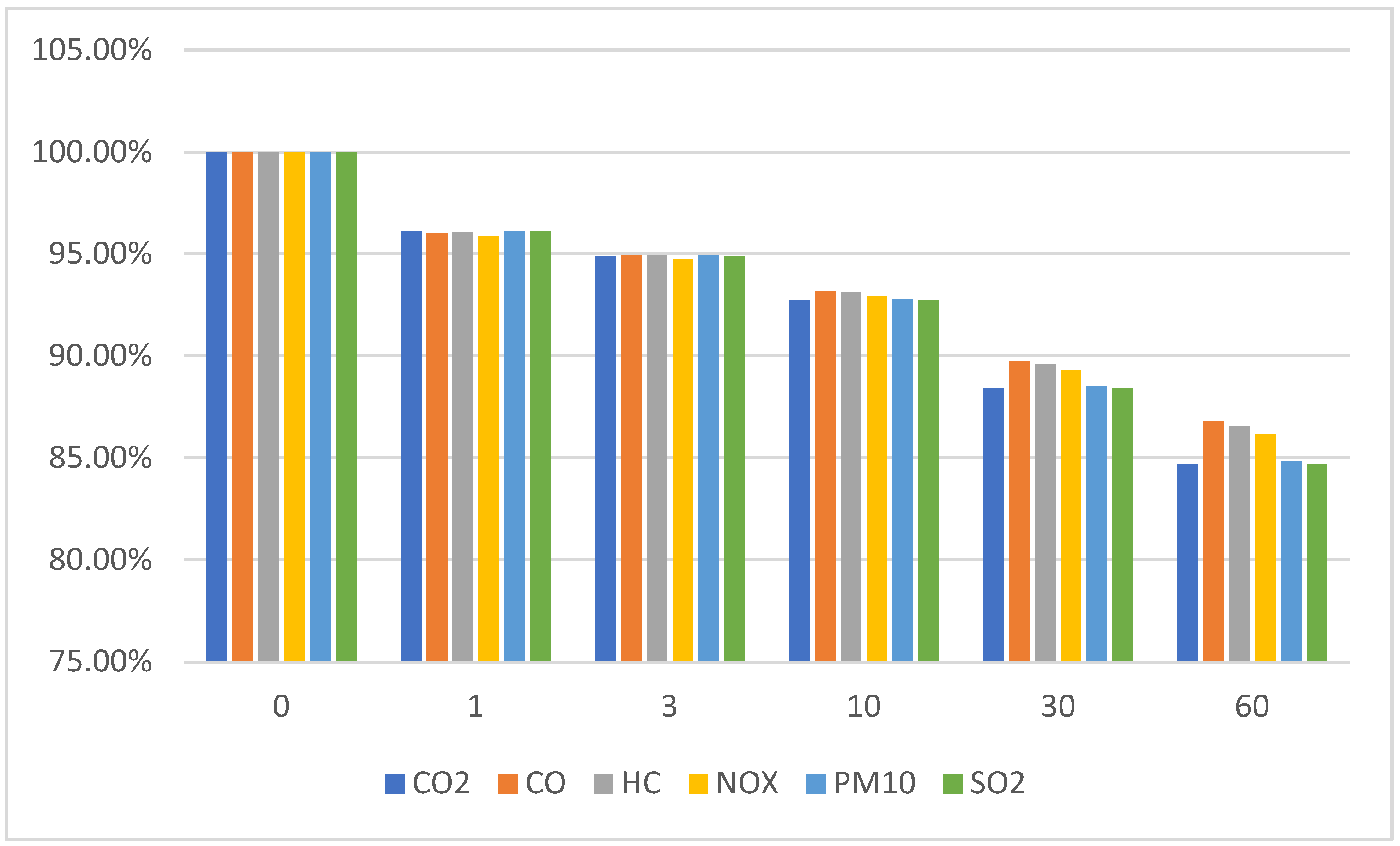
(4) The sums of the emissions from the six ships were calculated for CO2, CO, HC, NOX, PM10, and SO2. Then, the ratios of the sums with thinning at the different time intervals and without thinning were calculated (see the sum emissions in Table 3) and they are shown in Figure 6. When the time interval is 3 min, the ratios are 94.74–94.91%; when the time interval is 10 min, the ratios are 92.73–93.14%; when the time interval is 30 min, the ratios are 88.40–89.74%; and when the time interval is 60 min, the ratios are 84.69–86.80%.
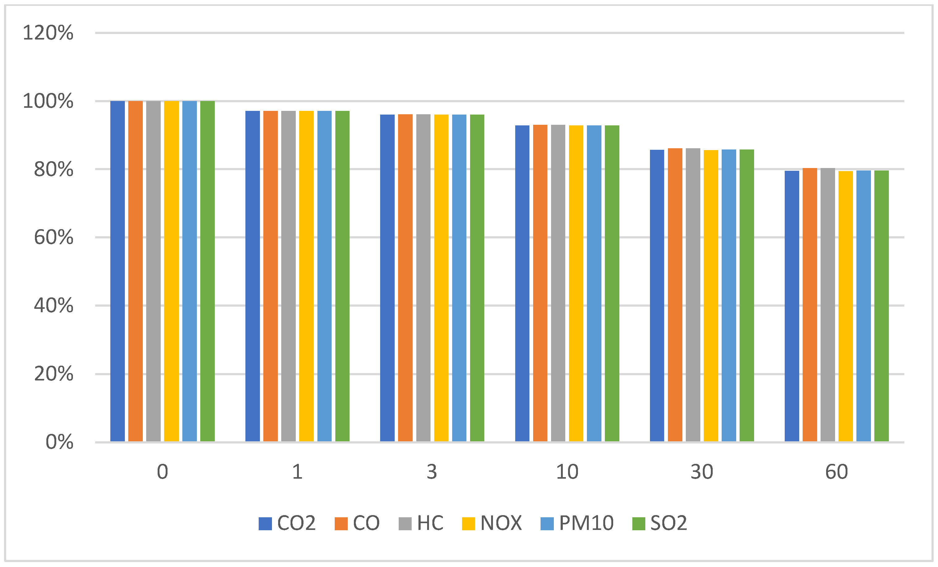
(5) The ratios of emissions from the six ships with thinning at the different time intervals and without thinning were calculated, then the average ratios were calculated and they are shown in Figure 7. When the thinning interval is more than 3 min, the impact of thinning is only about 4%, but the impacts increase to about 7% at 10 min, 14% at 30 min, and 20% at 60 min (Figure 7 and Figures S6–S10 in Supplementary Materials).
4. Discussion and Conclusions
(1) Thinning will lead to a smaller assessed emissions inventory. The data in Figure 3, Figure 4, Figure 5, Figure 6 and Figure 7 show that the thinning of AIS data has a significant impact on the air pollutant emission inventory not only for one day but also for one year, and the impact on the inventory increases with an increase in the data thinning time interval. When the thinning interval is less than 3 min, the impact is less than 5%, but the impact increases with longer intervals to about 10% at 10 min, 10–15% at 30 min, and 15–20% at 60 min.
(2) The thinning of AIS data has a more significant impact on the emission inventories of ships with acutely fluctuating speeds, such as in-and-out port ships and maneuvering ships (Figure 4a–d). It has less impact on the emission inventories of ships with constant speeds (Figure 4e–f). The main reason for the effect of AIS data thinning on the emission inventory is that the ships always sail at non-uniform speeds.
(3) In view of the large number and complexities of channels and ships in the world, the large amount of AIS data is a difficult problem that needs to be solved in establishing ship air pollutant emissions inventories. Data thinning is an effective method to reduce the number of calculations. However, the ideal thinning intervals need to be determined according to the inventory accuracy and the spatial scale. When establishing a coastal or national-scale ship air pollutant emissions inventory, the AIS data should be thinned at intervals of 3 min or 10 min. When establishing an air pollutant emissions inventory of inland ships, the AIS data should be thinned at an interval of less than 3 min. Thinning of the data is not recommended when establishing a port or small-scale ship air pollutant emissions inventory.
Supplementary Materials
The following supporting information can be downloaded at: https://www.mdpi.com/article/10.3390/atmos13071135/s1, Figure S1. Emissions of CO for the six ships in one day without thinning and with thinning at time interval of 1, 3, 10, 30, 60 mins; Figure S2. Emissions of HC for the six ships in one day without thinning and with thinning at time interval of 1, 3, 10, 30, 60 mins; Figure S3. Emissions of NOX for the six ships in one day without thinning and with thinning at time interval of 1, 3, 10, 30, 60 mins; Figure S4. Emissions of PM10 for the six ships in one day without thinning and with thinning at time interval of 1, 3, 10, 30, 60 mins; Figure S5. Emissions of SO2 for the six ships in one day without thinning and with thinning at time interval of 1, 3, 10, 30, 60 mins; Figure S6. Emissions of CO for the six ships in one year without thinning and with thinning at time interval of 1, 3, 10, 30, 60 mins; Figure S7. Emissions of HC for the six ships in one year without thinning and with thinning at time interval of 1, 3, 10, 30, 60 mins; Figure S8. Emissions of NOX for the six ships in one year without thinning and with thinning at time interval of 1, 3, 10, 30, 60 mins; Figure S9. Emissions of PM10 for the six ships in one year without thinning and with thinning at time interval of 1, 3, 10, 30, 60 mins; Figure S10. Emissions of SO2 for the six ships in one year without thinning and with thinning at time interval of 1, 3, 10, 30, 60 mins.
Author Contributions
Y.T. proposed the concepts. L.R. and H.W. designed the research methodology. L.R. performed the data analysis. Y.Y. wrote the calculation program. T.L. is responsible for the formal analysis and supervision. Y.T. and L.R. wrote the original draft. Y.Z. and H.W. reviewed and edited the manuscript. All authors have read and agreed to the published version of the manuscript.
Funding
This research was funded by the Key-Area Research and Development Program of Guangdong Province (Grant no. 2020B1111360001) and the National Natural Science Foundation of China (Grant no. 42077195).
Institutional Review Board Statement
Not applicable.
Informed Consent Statement
Not applicable.
Data Availability Statement
The data that support the findings of this study are available upon request from the corresponding author.
Conflicts of Interest
The authors declare no conflict of interest.
References
- Goldsworthy, L.; Goldsworthy, B. Modelling of ship engine exhaust emissions in ports and extensive coastal waters based on terrestrial AIS data—An Australian case study. Environ. Model. Softw. 2015, 63, 45–60. [Google Scholar] [CrossRef]
- Aksoyoglu, S.; Baltensperger, U.; Prév?T, A.S. Contribution of ship emissions to the concentration and deposition of air pollutants in Europe. Atmos. Chem. Phys. 2016, 16, 1895–1906. [Google Scholar] [CrossRef] [Green Version]
- Brandt, J.; Silver, D.J.; Christensen, H.J.; Andersen, S.M.; Bnlkke, H.J.; Sigsgaard, T. Assessment of past, present and future health-cost externalities of air pollution in Europe and the contribution from international ship traffic using the EVA model system. Atmos. Chem. Phys. 2013, 13, 7747–7764. [Google Scholar] [CrossRef] [Green Version]
- The Research Group of the Second National Pollution Source Census. Mobile Source Census Technical Specifications Formulating, and Organizing and Implementing Pollutant Emissions Accounting from Ships for the Second National Pollution Source Census. China Waterborne Transport Research Institute: Beijing, China, 2019. Available online: https://www.mee.gov.cn/xxgk2018/xxgk/xxgk01/202006/t20200610_783547.html (accessed on 10 May 2022).
- Liu, H.; Shang, Y.; Jin, X.-X.; Fu, X.-L. Review of methods and progress on shipping emission inventory studies. J. Environ. Sci. 2018, 38, 1–12. (In Chinese) [Google Scholar] [CrossRef] [PubMed]
- Olivier, J.; Peters, J. International Marine and Aviation Bunker Fuel: Trends, Ranking of Countries and Comparison with National CO2 Emissions; RIVM Report 773301002; National Institute of Public Health and the Environment (RIVM): Catharijnesingel, The Netherlands, 1999; Available online: http://www.rivm.nl/bibliotheek/rapporten/773301002.pdf (accessed on 10 May 2022).
- Dentener, F.; Drevet, J.; Lamarque, J.F.; Bey, I.; Eickhout, B.; Fiore, A.M.; Hauglustaine, D.; Horowitz, L.W.; Krol, M.; Kulshrestha, U.C.; et al. Nitrogen and sulfur deposition on regional and global scales: A multimodel evaluation. Glob. Biogeochem. Cycles 2006, 20, 16615. [Google Scholar] [CrossRef]
- Jalkanen, J.P.; Johansson, L.; Kukkonen, J.; Brink, A.; Kalli, J.; Stipa, T. Extension of an assessment model of ship traffic exhaust emissions for particulate matter and carbon monoxide. Atmos. Chem. Phys. 2012, 12, 2641–2659. [Google Scholar] [CrossRef] [Green Version]
- International Maritime Organization. The 2ed IMO GHG Study 2014; International Maritime Organization: London, UK, 2009. [Google Scholar]
- Yang, D.; Kwan, S.H.; Lu, T.; Fu, Q.; Cheng, J.; Streets, D.G.; Wu, Y.; Li, J. An Emission Inventory of Marine Vessels in Shanghai in 2003. Environ. Sci. Technol. 2007, 41, 5183–5190. [Google Scholar] [CrossRef] [PubMed]
- Fu, Q.Y.; Shen, Y.; Zhang, J. On the ship pollutant emission inventory in Shanghai port. J. Saf. Environ. 2012, 12, 57–64. (In Chinese) [Google Scholar]
- Li, Z.; He, L. Emission inventory estimation methods study of ship pollutants. Guangxi. J. Light Ind. 2011, 150, 79–80. (In Chinese) [Google Scholar]
- Ng, S.K.W.; Loh, C.; Lin, C.; Booth, V.; Chan, J.W.M.; Yip, A.C.K.; Li, Y.; Lau, A.K.H. Policy change driven by an AIS-assisted marine emission inventory in HongKong and the Pearl River Delta. Atmos. Environ. 2013, 76, 102–112. [Google Scholar] [CrossRef]
- Chen, D.-S.; Zhao, Y.-H.; Nelson, P.; Li, Y.; Wang, X.-T.; Zhou, Y.; Lang, J.-L.; Guo, X.-R. Estimating ship emissions based on AIS data for port of Tianjin, China. Atmos. Environ. 2016, 145, 10–18. [Google Scholar] [CrossRef]
- Wang, J.; Huang, Z.; Liu, Y.-Y.; Chen, S.-Y.; Wu, Y.-C.; He, Y.-Y.; Yang, X.-Y. Vessels’ Air Pollutant Emissions Inventory and Emission Characteristics in the Xiamen Emission Control Area. Environ. Sci. 2020, 41, 3572–3580. (In Chinese) [Google Scholar]
- Tokuslu, A. Assessment of Environmental Costs of Ship Emissions: Case Study on the Samsun Port. Environ. Eng. Manag. J. 2021, 20, 739–747. [Google Scholar] [CrossRef]
- Toscano, D.; Murena, F.; Quaranta, F.; Mocerino, L. Assessment of the impact of ship emissions on air quality based on a complete annual emission inventory using AIS data for the port of Naples. Sci. Total Environ. 2021, 232, 146869. [Google Scholar] [CrossRef]
- Yang, L.; Zhang, Q.; Zhang, Y.; Lv, Z.; Mao, H. An AIS-based emission inventory and the impact on air quality in Tianjin port based on localized emission factors. Sci. Total Environ. 2021, 783, 146869. [Google Scholar] [CrossRef] [PubMed]
- Zhao, J.-R.; Zhang, Y.; Patton, A.P.; Ma, W.-C.; Kan, H.-D.; Wu, L.-B.; Fung, F.; Wang, S.-X.; Ding, D.; Walker, K. Projection of ship emissions and their impact on air quality in 2030 in Yangtze River delta, China. Environ. Pollut. 2020, 263, 114643. [Google Scholar] [CrossRef] [PubMed]
- Zhou, Y.; Zhang, Y.; Ma, D.; Lu, J.; Luo, W.; Fu, Y.; Li, S.; Feng, J.; Huang, C.; Ge, W. Port-Related Emissions, Environmental Impacts and Their Implication on Green Traffic Policy in Shanghai. Sustainability 2020, 12, 4162. [Google Scholar] [CrossRef]
- EPA. Nonroad Engine and Vehicle Emission: Study Report and Appendixes—Draft Report; Technical Report; EPA: Frankfurt, Germany, 1991. [Google Scholar]
- Perez, H.M.; Chang, R.; Billings, R.; Kosub, T.L. Automatic Identification Systems (AIS) Data Use in Marine Vessel Emission Estimation. In Proceedings of the 18th Annual International Emissions Inventory Conference, Baltimore, MD, USA, 14–17 April 2009. [Google Scholar]
- International Maritime Organization. The Third IMO GHG Study 2014; International Maritime Organization: London, UK, 2014. [Google Scholar]
- Li, C.; Yuan, Z.-B.; Ou, J.-M.; Fan, X.-L.; Ye, S.-Q.; Xiao, T.; Shi, Y.-Q.; Huang, Z.-J.; Ng, S.K.W.; Zhong, Z.-M.; et al. An AIS-based high-resolution ship emission inventory and its uncertainty in Pearl River Delta region, China. Sci. Total Environ. 2016, 573, 1–10. [Google Scholar] [CrossRef] [PubMed]
- Fan, Q.-Z.; Zhang, Y.; Ma, W.C.; Ma, H.-X.; Feng, J.-L.; Yu, Q.; Yang, X.; Ng, S.K.W.; Fu, Q.-Y.; Chen, L.-M. Spatial and seasonal dynamics of ship emissions over the Yangtze River Delta and East China Sea and their potential environ-mental influence. Environ. Sci. Technol. 2016, 50, 1322–1329. [Google Scholar] [CrossRef] [PubMed]
- Jalkanen, J.P.; Brink, A.; Kalli, J.; Pettersson, H.; Kukkonen, J.; Stipa, T. A modelling system for the exhaust emissions of marine traffic and its application in the baltic sea area. Atmos. Chem. Phys. 2009, 9, 9209–9223. [Google Scholar] [CrossRef] [Green Version]
Figure 1.
Speeds of the six sampled ships throughout the sample day.

Figure 2.
Tracks of the sampled ships in 2019.

Figure 3.
Principle of data thinning.

Figure 4.
Emissions of CO2 for the six ships in one day without thinning (0 min) and with thinning at time intervals of 1, 3, 10, 30, and 60 min. (a) Ship 1 (b) Ship 2 (c) Ship 3 (d) Ship 4 (e) Ship 5 (f) Ship 6.
Figure 4.
Emissions of CO2 for the six ships in one day without thinning (0 min) and with thinning at time intervals of 1, 3, 10, 30, and 60 min. (a) Ship 1 (b) Ship 2 (c) Ship 3 (d) Ship 4 (e) Ship 5 (f) Ship 6.


Figure 5.
Emissions of CO2 for the six ships in one year without thinning (0 min) and with thinning at time intervals of 1, 3, 10, 30, and 60 min. (a) Ship 1 (b) Ship 2 (c) Ship 3 (d) Ship 4 (e) Ship 5 (f) Ship 6.
Figure 5.
Emissions of CO2 for the six ships in one year without thinning (0 min) and with thinning at time intervals of 1, 3, 10, 30, and 60 min. (a) Ship 1 (b) Ship 2 (c) Ship 3 (d) Ship 4 (e) Ship 5 (f) Ship 6.

Figure 6.
Ratios of the total emissions of CO2, CO, HC, NOX, PM10, and SO2 for the six ships in one year with thinning at different time intervals and without thinning.
Figure 6.
Ratios of the total emissions of CO2, CO, HC, NOX, PM10, and SO2 for the six ships in one year with thinning at different time intervals and without thinning.

Figure 7.
Average ratios of emissions of CO2, CO, HC, NOX, PM10, and SO2 from the six ships in one year with thinning at different time intervals and without thinning.
Figure 7.
Average ratios of emissions of CO2, CO, HC, NOX, PM10, and SO2 from the six ships in one year with thinning at different time intervals and without thinning.


Table 1.
Information on the sampled ships.
| Ship Number | MMSI | Navigation Status | Power of Main Engine (Kw) | Design Maximum Speed (Knots) |
|---|---|---|---|---|
| 1 | 353498000 | maneuvering | 2000 | 13.50 |
| 2 | 412044760 | maneuvering | 5736 | 14.75 |
| 3 | 412379280 | in-and-out port | 15,120 | 15.00 |
| 4 | 412379830 | in-and-out port | 15,120 | 15.00 |
| 5 | 413050000 | cruising | 54,720 | 25.70 |
| 6 | 413055000 | cruising | 36,480 | 24.20 |
Table 2.
Effect of thinning the AIS data on ship emissions inventories for one day at different time intervals.
Table 2.
Effect of thinning the AIS data on ship emissions inventories for one day at different time intervals.
| Ship Number | Time Interval (min) | Air Pollution Emissions (t) | |||||
|---|---|---|---|---|---|---|---|
| CO2 | CO | HC | NOX | PM10 | SO2 | ||
| 1 | 0 | 0.8442 | 0.0015 | 0.0007 | 0.0171 | 0.0005 | 0.0026 |
| 1 | 0.8435 | 0.0015 | 0.0007 | 0.0171 | 0.0005 | 0.0026 | |
| 3 | 0.8425 | 0.0015 | 0.0007 | 0.0171 | 0.0005 | 0.0026 | |
| 10 | 0.8355 | 0.0015 | 0.0007 | 0.017 | 0.0005 | 0.0026 | |
| 30 | 0.7946 | 0.0014 | 0.0007 | 0.0161 | 0.0005 | 0.0024 | |
| 60 | 0.6818 | 0.0013 | 0.0006 | 0.0138 | 0.0004 | 0.0021 | |
| 2 | 0 | 2.7308 | 0.0048 | 0.0022 | 0.0555 | 0.0016 | 0.0084 |
| 1 | 2.6982 | 0.0048 | 0.0022 | 0.0549 | 0.0016 | 0.0083 | |
| 3 | 2.6677 | 0.0047 | 0.0021 | 0.0542 | 0.0016 | 0.0082 | |
| 10 | 2.5154 | 0.0045 | 0.002 | 0.0511 | 0.0015 | 0.0077 | |
| 30 | 2.1392 | 0.0038 | 0.0017 | 0.0434 | 0.0013 | 0.0066 | |
| 60 | 1.5648 | 0.0028 | 0.0013 | 0.0317 | 0.0009 | 0.0048 | |
| 3 | 0 | 14.3691 | 0.025 | 0.0114 | 0.2927 | 0.0085 | 0.044 |
| 1 | 14.2225 | 0.0248 | 0.0113 | 0.2897 | 0.0084 | 0.0436 | |
| 3 | 13.5242 | 0.0236 | 0.0107 | 0.2754 | 0.008 | 0.0414 | |
| 10 | 11.2162 | 0.0198 | 0.009 | 0.2281 | 0.0066 | 0.0344 | |
| 30 | 8.4511 | 0.015 | 0.0068 | 0.1717 | 0.005 | 0.0259 | |
| 60 | 7.9612 | 0.0143 | 0.0065 | 0.1616 | 0.0047 | 0.0244 | |
| 4 | 0 | 38.571 | 0.0659 | 0.03 | 0.7877 | 0.0227 | 0.1182 |
| 1 | 38.4256 | 0.0657 | 0.0299 | 0.7847 | 0.0226 | 0.1178 | |
| 3 | 38.0748 | 0.0651 | 0.0296 | 0.7775 | 0.0224 | 0.1167 | |
| 10 | 35.8932 | 0.0614 | 0.0279 | 0.7329 | 0.0211 | 0.11 | |
| 30 | 32.6486 | 0.0563 | 0.0256 | 0.666 | 0.0192 | 0.1001 | |
| 60 | 28.3502 | 0.0493 | 0.0224 | 0.5776 | 0.0167 | 0.0869 | |
| 5 | 0 | 126.4682 | 0.3204 | 0.1373 | 3.6223 | 0.0758 | 0.3888 |
| 1 | 126.3367 | 0.32 | 0.1371 | 3.6186 | 0.0757 | 0.3884 | |
| 3 | 126.1431 | 0.3195 | 0.1369 | 3.6132 | 0.0756 | 0.3878 | |
| 10 | 126.0959 | 0.3193 | 0.1369 | 3.6121 | 0.0756 | 0.3876 | |
| 30 | 126.154 | 0.3195 | 0.1369 | 3.6135 | 0.0756 | 0.3878 | |
| 60 | 126.6537 | 0.3208 | 0.1375 | 3.6287 | 0.0759 | 0.3893 | |
| 6 | 0 | 110.3725 | 0.2638 | 0.113 | 3.1866 | 0.0657 | 0.3393 |
| 1 | 110.3043 | 0.2631 | 0.1128 | 3.1847 | 0.0656 | 0.3391 | |
| 3 | 110.3133 | 0.2632 | 0.1128 | 3.1849 | 0.0656 | 0.3391 | |
| 10 | 110.3044 | 0.263 | 0.1127 | 3.1848 | 0.0656 | 0.3391 | |
| 30 | 110.1606 | 0.2623 | 0.1124 | 3.1806 | 0.0655 | 0.3386 | |
| 60 | 109.7978 | 0.2611 | 0.1119 | 3.1702 | 0.0653 | 0.3375 | |
Table 3.
Effect of thinning the AIS data on ship emissions inventories for one year at different time intervals.
Table 3.
Effect of thinning the AIS data on ship emissions inventories for one year at different time intervals.
| Ship Number | Time Interval (min) | Air Pollution Emissions 1 (%) | |||||
|---|---|---|---|---|---|---|---|
| CO2 | CO | HC | NOX | PM10 | SO2 | ||
| 1 | 0 1 | 100.00 | 100.00 | 100.00 | 100.00 | 100.00 | 100.00 |
| 1 | 95.48 | 95.56 | 95.56 | 95.47 | 95.49 | 95.49 | |
| 3 | 95.41 | 95.50 | 95.50 | 95.40 | 95.43 | 95.43 | |
| 10 | 94.17 | 94.27 | 94.27 | 94.15 | 94.18 | 94.18 | |
| 30 | 89.79 | 89.94 | 89.94 | 89.77 | 89.81 | 89.81 | |
| 60 | 87.49 | 87.63 | 87.63 | 87.47 | 87.51 | 87.51 | |
| 2 | 0 | 100.00 | 100.00 | 100.00 | 100.00 | 100.00 | 100.00 |
| 1 | 99.67 | 99.67 | 99.67 | 99.68 | 99.68 | 99.68 | |
| 3 | 99.02 | 99.06 | 99.06 | 99.03 | 99.04 | 99.04 | |
| 10 | 95.48 | 95.69 | 95.69 | 95.46 | 95.52 | 95.52 | |
| 30 | 85.67 | 86.59 | 86.59 | 85.56 | 85.79 | 85.79 | |
| 60 | 74.90 | 77.03 | 77.03 | 74.63 | 75.17 | 75.17 | |
| 3 | 0 | 100.00 | 100.00 | 100.00 | 100.00 | 100.00 | 100.00 |
| 1 | 99.03 | 99.04 | 99.04 | 99.02 | 99.03 | 99.03 | |
| 3 | 97.24 | 97.28 | 97.28 | 97.24 | 97.25 | 97.25 | |
| 10 | 90.62 | 90.81 | 90.81 | 90.60 | 90.65 | 90.65 | |
| 30 | 77.56 | 78.25 | 78.25 | 77.48 | 77.65 | 77.65 | |
| 60 | 66.75 | 67.84 | 67.84 | 66.62 | 66.89 | 66.89 | |
| 4 | 0 | 100.00 | 100.00 | 100.00 | 100.00 | 100.00 | 100.00 |
| 1 | 97.12 | 97.14 | 97.14 | 97.12 | 97.12 | 97.12 | |
| 3 | 95.16 | 95.21 | 95.21 | 95.16 | 95.17 | 95.17 | |
| 10 | 89.03 | 89.21 | 89.21 | 89.01 | 89.05 | 89.05 | |
| 30 | 75.62 | 76.24 | 76.24 | 75.54 | 75.70 | 75.70 | |
| 60 | 64.56 | 65.64 | 65.64 | 64.43 | 64.70 | 64.70 | |
| 5 | 0 | 100.00 | 100.00 | 100.00 | 100.00 | 100.00 | 100.00 |
| 1 | 93.38 | 93.54 | 93.54 | 93.37 | 93.41 | 93.41 | |
| 3 | 92.36 | 92.52 | 92.52 | 92.34 | 92.38 | 92.38 | |
| 10 | 91.48 | 91.66 | 91.66 | 91.46 | 91.51 | 91.51 | |
| 30 | 90.23 | 90.50 | 90.50 | 90.20 | 90.27 | 90.27 | |
| 60 | 88.76 | 89.03 | 89.03 | 88.73 | 88.80 | 88.80 | |
| 6 | 0 | 100.00 | 100.00 | 100.00 | 100.00 | 100.00 | 100.00 |
| 1 | 97.57 | 97.67 | 97.67 | 97.55 | 97.58 | 97.58 | |
| 3 | 96.62 | 96.77 | 96.77 | 96.59 | 96.63 | 96.63 | |
| 10 | 96.09 | 96.28 | 96.28 | 96.06 | 96.11 | 96.11 | |
| 30 | 95.11 | 95.34 | 95.34 | 95.07 | 95.13 | 95.13 | |
| 60 | 94.61 | 94.86 | 94.86 | 94.57 | 94.64 | 94.64 | |
| Sum emission | 0 | 100.00 | 100.00 | 100.00 | 100.00 | 100.00 | 100.00 |
| 1 | 96.08 | 96.02 | 96.05 | 95.89 | 96.09 | 96.10 | |
| 3 | 94.89 | 94.91 | 94.93 | 94.74 | 94.91 | 94.91 | |
| 10 | 92.73 | 93.14 | 93.11 | 92.90 | 92.76 | 92.76 | |
| 30 | 88.40 | 89.74 | 89.60 | 89.29 | 88.50 | 88.48 | |
| 60 | 84.69 | 86.80 | 86.56 | 86.17 | 84.83 | 84.80 | |
1 The percentages assume that the emission value without thinning is 1, and the emission value with thinning is the ratio of the values with and without thinning.
Publisher’s Note: MDPI stays neutral with regard to jurisdictional claims in published maps and institutional affiliations. |
© 2022 by the authors. Licensee MDPI, Basel, Switzerland. This article is an open access article distributed under the terms and conditions of the Creative Commons Attribution (CC BY) license (https://creativecommons.org/licenses/by/4.0/).
Share and Cite
MDPI and ACS Style
Tian, Y.; Ren, L.; Wang, H.; Li, T.; Yuan, Y.; Zhang, Y. Impact of AIS Data Thinning on Ship Air Pollutant Emissions Inventories. Atmosphere 2022, 13, 1135. https://doi.org/10.3390/atmos13071135
AMA Style
Tian Y, Ren L, Wang H, Li T, Yuan Y, Zhang Y. Impact of AIS Data Thinning on Ship Air Pollutant Emissions Inventories. Atmosphere. 2022; 13(7):1135. https://doi.org/10.3390/atmos13071135
Chicago/Turabian StyleTian, Yujun, Lili Ren, Hongyan Wang, Tao Li, Yupeng Yuan, and Yan Zhang. 2022. "Impact of AIS Data Thinning on Ship Air Pollutant Emissions Inventories" Atmosphere 13, no. 7: 1135. https://doi.org/10.3390/atmos13071135
Note that from the first issue of 2016, this journal uses article numbers instead of page numbers. See further details here.