On the Redox-Activity and Health-Effects of Atmospheric Primary and Secondary Aerosol: Phenomenology

Abstract

The RHAPS (Redox-Activity And Health-Effects Of Atmospheric Primary And Secondary Aerosol) project was launched in 2019 with the major objective of identifying specific properties of the fine atmospheric aerosol from combustion sources that are responsible for toxicological effects and can be used as new metrics for health-related outdoor pollution studies. In this paper, we present the overall methodology of RHAPS and introduce the phenomenology and the first data observed. A comprehensive physico-chemical aerosol characterization has been achieved by means of high-time resolution measurements (e.g., number size distributions, refractory chemical components, elemental composition) and low-time resolution analyses (e.g., oxidative potential, toxicological assays, chemical composition). Preliminary results indicate that, at the real atmospheric conditions observed (i.e., daily PM₁ from less than 4 to more than 50 μg m⁻³), high/low mass concentrations of PM₁, as well as black carbon (BC) and water soluble Oxidative Potential (WSOP,) do not necessarily translate into high/low toxicity. Notably, these findings were observed during a variety of atmospheric conditions and aerosol properties and with different toxicological assessments. Findings suggest a higher complexity in the relations observed between atmospheric aerosol and toxicological endpoints that go beyond the currently used PM₁ metrics. Finally, we provide an outlook to companion papers where data will be analyzed in more detail, with the focus on source apportionment of PM₁ and the role of source emissions on aerosol toxicity, the OP as a predictive variable for PM₁ toxicity, and the related role of SOA possessing redox-active capacity, exposure-response relationships for PM₁, and air quality models to forecast PM₁ toxicity.

1. Introduction

Ambient air pollution is the leading environmental risk factor globally. The WHO estimates that exposure to air pollution might be associated with around 7 million deaths, especially from noncommunicable cardiovascular and respiratory diseases [1]. Among air pollutants, PM_2.5 (particulate matter with an aerodynamic particle diameter less than 2.5 μm) has received special attention. To date, there is evidence of causal relationships between exposure to PM_2.5 air pollution and all-cause mortality, as well as several diseases, including lung cancer, stroke, respiratory infections, and pulmonary diseases [1,2]. However, our understanding of this relationship is not clear enough.

In 2021, the WHO recommended lowering the PM_2.5 annual air quality guideline level from 10 to 5 μg m⁻³ to reflect the new evidence about effects occurring at low levels of exposure. Indeed, recent outcomes from seven large prospective cohort studies in Europe focusing on low PM_2.5 concentrations showed positive associations between long-term exposure to low PM_2.5 and non-accidental, cardiovascular, non-malignant respiratory, and lung cancer mortality without an indication of a lower threshold (below 1–5 μg m⁻³) [3]. Among the reasons possibly explaining the occurrence of health effects even at these very low doses, there is the fact that these studies are based on PM_2.5 mass, a metric that is not ideal for representing the “biologically-active dose” of toxic PM_2.5. In fact, PM_2.5 being the same, health impacts can vary significantly depending on the blend of particles and gaseous compounds, as well as additional factors such as mixing, weather, atmospheric chemistry, etc. [4]. Indeed, PM_2.5 is characterized by a blend of components, complex mixtures of interacting different types from many emission sources, with physicochemical properties significantly varying in time and space that undergo fast atmospheric transformation processes and thus may have very diverse toxicological properties. In 2021, WHO prioritized specific types of PM, i.e., Black Carbon (BC), Elemental Carbon (EC), sand and dust storm particles, and Ultrafine Particles (UFPs) but concluded that the quantitative evidence on independent adverse health effects from these pollutants was still insufficient for new Air quality guideline (AQG) levels [1]. Additionally, a number of studies [5] have highlighted the toxicological potential of secondary organic aerosols (SOA). This discovery demonstrated that ambient aerosols responsible for potential impacts on human health are not only emitted from pollution hotspots. After emission, new toxic compounds can be formed in the atmosphere, the toxicological properties varying as a function of environmental conditions, such as temperature, solar irradiance [6], and availability of liquid water in the form of fog/cloud droplets or deliquesced aerosols [7]. It is worth noting that seasonal differences in toxicological response were observed, e.g., in the TOBICUP (TOxicity of BIomass Combustion generated Ultrafine Particles) project when summer vs. winter ambient samples of UFPs were assayed. Indeed, for UFP, summer samples induced a more pro-inflammatory response than wintertime ones; in contrast, winter UFP samples generated higher genotoxic effects [8,9,10]. The CARE field study (Carbonaceous aerosol in the Rome Environment) based in Rome during the winter season involved the deployment of a suite of highly time-resolved physical and chemical aerosol characterization along with in-field toxicological measurements [11,12]. The results show a complex relationship between PM_2.5 oxidative and pro-inflammatory properties and primary combustion aerosol concentrations and indicate that these are greatly impacted by changes in the size and aging state of the particles in the real atmosphere.

Among the several mechanisms of adverse cellular effects, there are oxygen-free radical-generating activity, DNA oxidative damage, mutagenicity, stimulation of pro-inflammatory factors, and the generation of reactive oxygen species (ROS). These received considerable attention from aerosol scientists, who found in ROS studies an opportunity to link aerosol composition to biological effects [13]. The best candidates for particulate compounds responsible for ROS activity encompass transition metals and specific organic compounds such as quinoid species [13]. Wide ranges of fuels and experimental conditions have been explored in the laboratory to assess the characteristics of combustion aerosols in terms of toxicological endpoints and mechanisms of action (e.g., ROS formation). According to [14] Lakey et al. (2016), the ROS activity of ambient aerosol is a broad function of the logarithm of PM concentrations with a tendency to level off at very high pollution levels. Other authors [15], comparing ROS assays performed on size-segregated PM samples from six cities on three continents, showed that finer aerosol size fractions tend to have a higher ROS activity and that chemical components determining ROS formation include several transition metals and polar organic compounds. Another experiment based in the Po Valley in wintertime showed that fog droplets exhibit a higher intrinsic ROS content with respect to the aerosol particles the fog is formed of [16], indicating that aqueous-phase reactions in deliquesced particles contribute to altering (possibly amplifying) the oxidative potential of PM. The role of PM-induced ROS in lung dysfunction and potentially adverse cardiovascular outcomes set the basis for the development of chemical (a-cellular) assays suitable for low-cost, widespread observations of ROS formation in ambient PM samples. Their use is considerably extending the data availability for proxies of ambient PM toxicity (linked to oxidative potential) in a variety of environments and for diverse source-related PM fractions [17]. The results of such studies suggest that atmospheric processing exerts a great impact on a parameter, the PM oxidative potential (OP), defined by the ability of aerosol particles to oxidize target (bio)molecules and tested as an alternative air quality metric in a few pilot studies [18], although it remains an object of intense research and discussion.

This is the context in which the RHAPS (Redox-Activity And Health-Effects Of Atmospheric Primary And Secondary Aerosol) project was launched in 2019. The major objective of RHAPS is to identify specific properties (or combinations of them) of PM₁ (particles with an aerodynamic diameter less than 1 μm) from combustion sources that are responsible for toxicological effects and can be used as new metrics for health-related outdoor pollution studies (Figure 1). Field campaigns and laboratory experiments in an atmospheric simulation chamber (see Supplementary Materials) were carried out with a focus on finding a link between the OP carried by SOA and PM₁ toxicity.

In this paper, we present the overall methodology of the RHAPS project and introduce the phenomenology and the first data observed, which will be discussed in detail in a series of companion papers.

2. Materials and Methods

2.1. Measurement Sites and Observational Periods

Field observations were carried out in the Po Valley (Italy) using a tandem urban–rural sites combination: BO, urban background, 44°31′29″ N, 11°20′27″ E) and San Pietro Capo Fiume (SPC, rural, 44°39′15″ N, 11°37′29″ E). There are two reasons to focus on the Po basin during RHAPS: (1) it is one of the major air pollution hotspots in Europe, and (2) it provides opportunities to investigate the processes regulating aerosol formation and redox activity in a polluted regional background atmosphere. In the rural Po Valley, aerosols are mainly emitted from residential wood burning and also formed in situ by secondary reactions involving ammonia (from agricultural emissions) and the photochemical products of NOx and VOCs (nitric acid and SOA, respectively).

Considering that PM₁-to-PM_2.5 average ratios in the investigated area were estimated at 60–80%, with lower values in summer vs. winter [19,20], it is interesting to note that the contribution of secondary sources in the regional background to PM_2.5 concentrations in the Po Valley varies between 50% (in the largest city, Milan [21]) to more than 70% in district cities and rural background sites [22,23]. The effect of the oxidative potential of SOA on the toxicological properties of the Po Valley aerosol is still poorly characterized. We demonstrated, however, that the concentration of the markers of oxidative stress in PM₁ in the rural Po Valley can be of the same order of magnitude as the concentrations reported for US megacities (Los Angeles) [16]. In the same area, fog water, which is enriched in SOA and depleted of transition metals with respect to the aerosol, showed the highest intrinsic redox activity. It is noteworthy that in summer, field measurements were run only at the background urban site, as the atmospheric mixing during the warm season is such that differences between the two sites are largely reduced.

Given the complexity of observing the phenomena, we elaborated a field measurement strategy combining different periods, combining intensive and super-intensive observational periods (

Table 1. Intensive and Super-Intensive Observational Periods (IOPs, SIOPs) during RHAPS.

ID	Winter	Summer
IOPs	21 January 2021–18 March 2021	8 June 2021–14 July 2021
SIOPs	26 January 2021–3 January 2021 2 February 2021–6 February 2021 16 February 2021–20 February 2021	29 June 2021–2 July 2021

).

During Intensive Observational Periods (IOPs), both daily measurements (from 8.00 a.m. to 8.00 a.m. local time, ca. 60 samples in winter and 35 in summer) and online and high-time resolution instrumentations were operated in parallel. In winter, IOP was conducted from 21 January to 18 March 2021, and in summer from 8 June to 14 July 2021.

A total of four Super-Intensive Observational Periods (SIOPs) were carried out during the project, each SIOP lasting four days (from h 8.00 a.m. to h 8.00 a.m. local time); three SIOPs were carried out in winter (January/February 2021), and one SIOP in summer (June/July 2021). The periods for the SIOPs were planned according to a proper strategy. First, to catch the accumulation of aerosols in the atmosphere, we aimed to have each SIOP lasting four consecutive “stable weather” days, starting from a “clean” day, i.e., good weather possibly following bad weather conditions. Second, to be consistent with emission source paths, we always started the SIOP on Tuesdays and ended on Saturdays. Finally, we aimed at having SIOPs days representative of four source-specific aerosol types: biomass burning (BB), urban aerosol (i.e., traffic emissions), secondary aerosols, and clean conditions. To proxy these aerosols, we selected a subset of variables, as described in

Table 2. Exemplary of variables used to identify source-specific aerosol types.

Variables	Urban	BB	SOA/SIA	Clean
BC-to-PM1	↑		↓
BC-to-OA	↑	↓	↓
AAE (467-660)	↓	↑
Nitrate mass concentration			↑	↓
Sulfate mass concentration			↑	↓
Primary OC mass concentration	↑	↑
Secondary OC mass concentration			↑
Median particle diameter	↓	↓	↑
PM1 mass concentration			↑	↓
BC mass concentration	↓	↑		↓
Number concentration	↑			↓
Secondary formaldehyde			↑
Weather conditions	stable	stable	Stable, foggy	Strong winds, low pressure, no rain

. The latter were selected according to our experience and knowledge of the measurement sites and the analysis of available experimental data obtained during the first part of the IOPs (i.e., PM₁ chemical components, particle number size distribution, and BC). Every week, we ran a proper air quality model to forecast weather conditions and these variables for the next week, and accordingly, we started (or not) the SIOP.

2.2. Aerosol and Meteorological Field Measurements

2.2.1. PM₁ Mass and Chemical Composition—Daily Samples Characterization

At both sites, many parallel sampling lines were deployed to collect samples devoted to a comprehensive aerosol chemical characterization in terms of mass concentration, elements, ions, and carbonaceous components (PAHs included), for OP assessment and toxicological assays (see

Table 3. Summary of sampling lines and filters used.

Winter Campaign (21 January 2021–18 March 2021)
Urban Background Site (BO)
Sampler	Flowrate	Inlet	Sampling Time	Filters	Target
Dual channel (Dadolab Gemini)	1.15 m3/h	Modified PM1	24 h from 8:00 to 08:00 LT	Quartz-fibre PTFE	Ions (by IC), levoglucosan (HPAEC-PAD) Elements (PIXE)
Dual channel (Dadolab Gemini)	1.15 m3/h	Modified PM1	24 h from 8:00 to 08:00 LT	2 PTFE	Toxicological assays and embryotoxicity
Single channel (Dadolab Giano)	1.15 m3/h	Modified PM1	24 h from 8:00 to 08:00 LT	PTFE	Water soluble oxidative potential
Single channel (Dadolab Giano)	1.15 m3/h	Modified PM1	24 h from 8:00 to 08:00 LT	PTFE	Trace metals (ICP-MS)
Single channel (TCR-Tecora Skypost)	1.15 m3/h	Modified PM1	24 h from 8:00 to 08:00 LT	Quartz fiber	Oxidative potential—OP tot
STRAS	0.5 m3/h	Modified PM1	1 h	Polycarbonate	1 h resolved elements (PIXE)
Single channel (TCR-Tecora Skypost)	2.3 m3/h	PM1	48 h from 8:00 to 08:00 LT	Pre-fired quartz fibre	14C
HV sampler (TCR-Tecora)	30 m3/h	PM1	24 h from 8:00 to 08:00 LT	Quartz fibre	Extra analyses
Rural background site (SPC)
Dual channel (Dadolab Gemini)	1.15 m3/h	Modified PM1	24 h from 8:00 to 08:00 LT	Quartz-fibre PTFE	Ions (by IC), levoglucosan (HPAEC-PAD) Elements (PIXE)
Dual channel (Dadolab Gemini)	1.15 m3/h	Modified PM1	24 h from 8:00 to 08:00 LT	2 PTFE	Toxicological assays and embryotoxicity
Dual channel (Dadolab Gemini)	1.15 m3/h	Modified PM1	24 h from 8:00 to 08:00 LT	2 PTFE	Water soluble oxidative potential Trace metals (ICP-MS)
Single channel (TCR-Tecora Skypost)	1.15 m3/h	Modified PM1	24 h from 8:00 to 08:00 LT	Quartz fiber	Oxidative potential—OP tot
STRAS	0.5 m3/h	Modified PM1	1 h	Polycarbonate	1 h resolved elements (PIXE)
SUMMER CAMPAIGN (08 June 2021–14 July 2021)
Urban background site (BO)
Dual channel (Dadolab Gemini)	2.3 m3/h	PM1	24 h from 8:00 to 08:00 LT	Quartz-fibre PTFE	Ions (by IC), levoglucosan (HPAEC-PAD) Elements (PIXE)
Dual channel (Dadolab Gemini)	2.3 m3/h	PM1	24 h from 8:00 to 08:00 LT	2 PTFE	Toxicological assays and embryotoxicity
Dual channel (Dadolab Gemini)	2.3 m3/h	PM1	24 h from 8:00 to 08:00 LT	2 PTFE	Water soluble oxidative potential Trace metals (ICP-MS)
STRAS	0.5 m3/h	Modified PM1	2 h	Polycarbonate	2 h resolved elements (PIXE)
Single channel (Dadolab Giano)	2.3 m3/h	PM1	24 h from 8:00 to 08:00 LT	Quartz fiber	Oxidative potential—OP tot
Single channel (TCR-Tecora Skypost)	2.3 m3/h	PM1	72 h from 8:00 to 08:00 LT	Pre-fired quartz fiber	14C
HV sampler (TCR-Tecora)	30 m3/h	PM1	24 h from 8:00 to 08:00 LT	Quartz fiber	Extra analyses

for a summary). PM₁ daily samples were collected on PTFE filters (Pall R2PJ047, Pall Life Sciences, Ann Arbor, MI, USA) and on pre-fired 47 mm diameter quartz fiber filters (Pallflex Tissuquartz 2500 QAO-UP, Pall Life Sciences, Ann Arbor MI, USA) according to the specific analysis foreseen for that sample, as reported in Table 3. A total of 813 daily samples were collected in winter and 234 in summer.

The low-volume samplers—many of them provided 2 parallel sampling lines—were operated at 1.15 m³/h during the winter campaign in order to avoid filter clogging and high pressure drops. To this aim, the sampling inlets were modified by plugging 8 out of 16 nozzles; on the contrary, the flowrate during the summer campaign was set at 2.3 m³/h, and no modifications to the standard 16 nozzles PM₁ inlet were done. An identical sampling configuration was adopted at both sites.

Mass concentration was gravimetrically determined on PTFE filters using a Sartorius microbalance with 1 μg sensitivity and equipped with an automatic sample changer.

PTFE filters were analyzed by PIXE analysis at the INFN-LABEC accelerator facility in Florence to obtain the elemental concentration of Z > 10 elements [24] and by ICP-MS (Bruker 820-MS, Billerica, MA, USA) at Sapienza University in Rome to retrieve the soluble and/or insoluble fraction of Al, As, Ba, Bi, Cd, Ce, Co, Cr, Cs, Cu, Fe, Ga, K, La, Li, Mn, Mo, Na, Pb, Rb, Sb, Sn, Ti, Tl, U, V, W, Zn, and Zr by applying a chemical fractionation procedure that increases the selectivity of the elements as source tracers [25]. Instrumental conditions and performance of the method are described in [26,27], respectively.

Punches from quartz fiber filters were analyzed at the University of Genoa with Ion Chromatography analysis for major ions (Cl⁻, NO₃⁻, SO₄²⁻, Na⁺, NH₄⁺, K⁺, Mg²⁺, Ca²⁺) [28] and for levoglucosan (1,6-Anhydro-beta-glucopyranose) with HPLC-PAD following [29]. Further details are reported in the Supplementary Materials.

Elemental and organic carbon fractions (EC and OC) were determined on one punch taken from 24 h quartz fiber filters by thermo-optical analysis with an offline OCEC Carbon Aerosol Analyser (Sunset Laboratory Inc., Tigard, OR, USA) by applying the NIOSH-QUARTZ temperature protocol.

PAHs, i.e., benzo(α)anthracene, chrysene, benzo(β)fluoranthene, and benzo(α)pyrene, were also evaluated in samples collected on quartz filters. The samples were prepared according to previous works [30,31] with some modifications. For the quantitative analysis, benz(α)anthracene-D12 was added as an internal standard (200 ng/sample) to all filters. The quantitative analysis was performed using gas chromatography (Varian 3900 GC) supplied by ion trap mass spectrometry (Varian Saturn 2100T). The chromatographic separation was achieved with the TG-5SILMS column. Further details can be found in the Supplementary Materials (Tables S1–S3).

2.2.2. Non-Refractory PM₁ Chemical Components (AMS)

The mass loading and chemical composition of submicron aerosol particles were obtained online by the High-Resolution Time-of-Flight Aerosol Mass Spectrometer (HR-TOF-AMS, Aerodyne Research) [32] at both locations. The HR-TOF-AMS provides measurements of the non-refractory sulfate, nitrate, ammonium, chloride, and organic mass of the submicron particles (NR-PM₁). The working principle of the HR-TOF-AMS is described in detail in [32,33,34]. Briefly, during all the campaigns, the HR-TOF-AMS was operating in “V” ion path modes every 2.5 min. The resolving power [35] of the V-ion mode was about 2000–2200 during all the campaigns.

Ionization efficiency (IE) calibrations were performed before and after every campaign and approximately once every two weeks during the campaigns. Filter blank acquisitions during the campaign were performed at least once a day to evaluate the background and correct for the gas-phase contribution. All data were analyzed using the standard ToF-AMS analysis software SQUIRREL v1.57 and PIKA v1.16 (D. Sueper, available at: http://cires.colorado.edu/jimenez-group/ToFAMSResources/ToFSoftware/index.html, accessed on 1 September 2021) within Igor Pro 6.2.1 (WaveMetrics, Lake Oswego, OR, USA). The HR-TOF-AMS collection efficiency (CE) was calculated based on aerosol composition, according to [36] and confirmed against parallel offline measurements. At both sampling stations, the aerosol was dried to about 35–40% by means of a Nafion drier before sampling with the HR-TOF-AMS.

2.2.3. Elemental Composition (STRAS)

High-time resolution samples were collected at both BO and SPC using the STRAS sampler (Size and Time-Resolved Aerosol Sampler), which was recently developed as an upgrade of the previous streaker sampler to collect the fine and coarse aerosol fractions with high-time resolution. In RHAPS, a PM₁ inlet was mounted on STRAS, and the particles were sampled with 1 h resolution during winter (for a total of 2352 time slots) and 2 h resolution during summer (for a total of 401 time slots) on a polycarbonate filter; each filter collects up to 168 samples corresponding to 1 week of hourly samples.

STRAS spots were analyzed by PIXE at the INFN-LABEC for offline high throughput determination of elements with Z > 10 [37].

2.2.4. Particle Number Size Distributions

The Particle Number Size Distribution (PNSD) was measured at the urban background site of BO by combining a Mobility Particle Size Spectrometer (TROPOS SMPS) equipped with a butanol-based condensation particle counter (CPC, model 3772, TSI Inc., Shoreview, MN, USA) and a commercial aerodynamic particle sizer (APS, TSI). Particles from 8 to 800 nm of electrical mobility diameter (d_m) were sized and counted by the SMPS; particles from 0.5 to 20 μm of aerodynamic diameter (d_a) were sized and counted by the APS. SMPS data were corrected for penetration errors through the sampling line (TROPOS-made software), penetration efficiency due to diffusion losses (calculated according to [38]) being higher than 98.92% for particles bigger than 15 nm. The aerosol sampling line was dried down to relative humidity of about 30% by means of a Nafion drier.

PM₁ mass concentration with 5 min time resolution was constructed from the PNSD data, according to the procedure described elsewhere [11]. In short, PM₁ was calculated from the particle volume size distribution under the hypothesis of spherical particles, and a size-dependent particle density varying from 1.25 to 1.5 g cm⁻³. The daily PM₁ from SMPS was then validated according to the daily PM₁ measured through the reference procedure, the goodness of fit being R² = 0.99 (Supplementary Materials, Figures S21 and S22).

2.2.5. Absorption and Scattering Coefficients (Aethalometer, PAX, DBAP, Filters)

Optical characterization of the daily samples collected at both sites on quartz fiber filters was performed by Multi-Wavelength Absorption Analyzer [39,40] to retrieve the absorption coefficients at 5 different wavelengths (λ = 850, 635, 532, 405, and 375 nm). A blank filter was used as reference for both winter and summer samples analysis.

In addition to the determination of Ångström Absorption Exponent (AAE) [41], previous research studies showed that multi-wavelength absorption coefficients were proved to be effective for apportioning contributions from fossil fuels and biomass burning combustion sources in aerosol samples [40,42]. The determined absorption coefficients were apportioned following the methodology presented in [40,43] and as previously employed in several field campaigns at urban and rural sites [44,45]. The methodology differentiates and quantifies the contribution to the total absorption of equivalent black carbon (eBC) emitted by wood-burning (eBC_WB) and fossil fuel (eBC_FF) as well as brown carbon (BrC) due to incomplete combustion.

During the winter campaign, two photoacoustic extinction meters (PAXs, Droplet Measurement Technologies, Boulder, CO, USA) provided the online determination of PM₁₀ absorption and scattering coefficients at λ = 532 and 405 nm, with 1 min resolution.

At the background urban site in Bologna, a 7-wavelength (370, 470, 520, 590, 660, 880, and 950 nm) aethalometer (model A33, Magee scientific [46]) provided eBC mass concentration and AAE with 1 min time resolution. According to the instrument manufacturer, the eBC mass concentration from AE33 was obtained from measurements at λ = 880 nm with a mass absorption coefficient of 7.77 m² g⁻¹ [46]. The aerosol sampling line was dried to about 20–30% by means of a Nafion drier.

At the rural site of SPC, a Dual Beam Absorption Photometer (DBAP) was used. DBAP5 is a 5-wavelength (from 420 to 870 nm) filter absorption photometer based on dual-beam technology that measures the absorption properties of the particulate matter. Starting from the measurement of the filter light transmission variation over time due to the particle load, it evaluates the attenuation coefficients; then, by applying the appropriate filter correction equations, it evaluates the absorption coefficient and the Equivalent Black Carbon concentration using the Mass Absorption Coefficients. Dual-beam technology is a technique that simultaneously compares the absorption of the particulate matter with the absorption on the white filter, providing more precise measurement, especially in low concentration sites.

2.2.6. EC and OC—Online Measurements

The EC and OC mass concentration with 2 h time resolution was obtained by a Sunset Field Thermal-Optical Analyzer (Model-4 Semi-Continuous OC-EC Field Analyzer—Sunset Laboratory Inc., Sunset Laboratory Inc. Tigard, OR, USA).

Briefly, this instrument collects PM on a quartz fiber filter and automatically analyses it at the end of each sampling period. The instrument inlet is equipped with a cyclone (cut point 1 μm) and a denuder for organics. In this campaign, a time resolution of 2 h (105 min of sampling followed by 15 min of analysis) was chosen as a compromise to get an adequate time resolution (comparable with that of other instruments used in this project) and a sufficient amount of collected sample mass (to maintain a good accuracy in the EC and OC quantification). The instrument was calibrated by sucrose standards, and the NIOSH protocol was used for thermal analysis.

Elemental and organic carbon (EC and OC) on the daily samples on quartz fiber filters were determined through thermal-optical transmission analysis with a Sunset EC/OC analyzer (Sunlab), using the NIOSH5040 protocol [47] corrected for temperature offsets. NIOSH5040 protocol lasts about 12 min, and the highest reached temperature is 940 °C. The instrument was calibrated with a TOC Standard Solution before starting the analysis.

2.2.7. Micrometeorology

To consider mean and turbulent atmospheric processes during the RHAPS field experiment, the meteorological variables (temperature, relative humidity, pressure, wind speed, solar radiation) were measured with a standard meteorological instrument (Lufft weather station WS700) with 1 min time resolution, while to measure the turbulence affecting the atmospheric processes near the surface, high-frequency measurements of the 3 wind components u, v, w, and virtual temperature T, were made with an ultrasonic thermometer-anemometer uSonic-3 by Metek (sampling frequency 10 Hz) installed at height z = 3.3 m a.g.l. From these measurements we computed the wind speed and direction as well as the fluctuations u′, v′, w′, and T_v′ with respect to the 1 h linearly detrended mean wind components (<u>, <v>, <w>) and virtual temperature <T_v> (u′ = u − <u>, v′ = v − <v>, w′ = w − <w>, T_v′ = T_v − <T_v>). We estimated the sensible heat flux H₀ = ρc_pw′T_v′ (ρ is the air density, c_p is the specific heat capacity of air at constant pressure) and turbulent kinetic energy TKE = 1/2 (u′² + v′² + w′²) and the stability parameter z/L, where L is the Obukhov length. H₀ provides a measure of the thermal mixing capability of the atmosphere. TKE represents the intensity of turbulence produced by fluid shear, friction or buoyancy, or through external forcing. As both H₀ and TKE vary significantly in time and in space, they need to be monitored continuously.

2.3. Toxicological Assessment

2.3.1. Oxidative and Reducing Potential

One sampling line operated with PTFE filters was devoted to oxidative and reducing potential assessment; each filter was extracted in 10 mL of deionized water by rotating agitation at 60 rpm for 30 min. The obtained solution was then filtered through a nitrocellulose filter and split into proper aliquots for the dithiothreitol (DTT), ascorbic acid (AA), and 2′,7′-dichlorofluorescein (DCFH) OP assays (OP^DTT, OP^AA, OP^DCFH) and for the 2,2-diphenyl-1-picrylhydrazyl (DPPH) reducing potential (RP) assay (RP^DPPH). The OP and RP analytical measurements followed the methods reported in [48,49,50].

The reducing potential assay is based on the use of the stable free radical DPPH (2,2-Diphenyl-1-picrylhydrazyl). The DPPH assay is a commonly used spectrophotometric method to estimate the antioxidant activity of several matrices, such as food and plants, by measuring the decrease of absorbance over time [51,52]. The DPPH is a stable free radical by virtue of the delocalization of the spare electron over the molecule [53], and it accepts electrons or hydrogen radicals from donor compounds [54]. DPPH shows a strong absorption band at 517 nm due to its odd electron, and solution appears a deep violet color. The resulting decolorization turning yellow is proportional to the number of electrons taken up [51].

A parallel sampling on quartz fiber filters was devoted to water-soluble and total OP determination by the dithiothreitol (DTT) assay. The adopted procedures are those by [55,56] Cho et al. (2005) and Verma et al. (2009), for the water-soluble OP, and by [57] Gao et al. (2017), for the total OP. For the water-soluble OP determination, filter portions were extracted in deionized water by gentle shaking (30 min), and the extracts were filtered using a PTFE 0.45 μm pore syringe filter to remove insoluble materials and filter debris.

For the determination of the total aerosol OP, the procedure was similar to the one described above, with only one notable difference. The quartz fiber filter aliquots were not removed from the extraction solution after the end of the extraction procedure, and they were kept in the primary vial while performing the DTT assay in order to allow both soluble (in the extract) and insoluble (attached to the filter) aerosol components to react with the DTT. Total OP determinations are still ongoing, and the results will not be discussed in the present work. More details about the experimental procedure are presented in the Supplementary Materials.

At the urban background site, high-time resolved (2 h time resolution) OP was measured through the 2′,7′-dichlorofluorescein (DCFH) assay (OP^DCFH) employing a particle-into-liquid sampler (PILS), which allows for continuous PM collection of a diluted solution of soluble species with suspended insoluble particles [58]. The sampling line was equipped with a PM₁ inlet and a denuder line to keep acid and basic gasses out of the sample. This technique does not guarantee the complete recovery of small and hydrophobic particles because particle growth is achieved through water condensation [59].

2.3.2. Filter-Based Toxicological Assays

To characterize the toxicological effects of PM₁ water extracted from PTFE filters, different in vitro models representative of human lung tissue and targeted cells were used (e.g., BEAS-2B, THP-1). In order to assure the comparability with OP measurements, the extraction procedure (see Supplementary Materials) was exactly the same and was carried out on the same days as toxicological measurements. Cells were exposed to increased dilutions of extracts for different times (30 min, 1, 3, and 24 h). After exposure, as an indicator of unwanted biological effects, cell viability (e.g., MTT reduction assay, PI staining, oxidative stress) and release of inflammatory mediators (e.g., IL-8), genotoxicity and mutagenicity (e.g., alkaline comet assay, micronucleus test) were investigated [8,60]. In parallel, to evaluate embryotoxicity, the effects of extracts were tested in Xenopus laevis embryos. Xenopus laevis embryos were exposed during the whole R-FETAX test period (from midblastula to tadpole, according to [61]) to the soluble extracted fraction diluted 1:10 in maintaining solution (see details in Supplementary Materials). At the end of the test, tadpoles were morphologically observed under a dissecting microscope (Leica). The developmental degree (to evaluate old- and young-for-age embryos) was evaluated according to [62] developmental scoring system adapted to Xenopus laevis considering the normal table of X. laevis development [63] (details in Supplementary Materials). Tadpole length was measured in order to evaluate small- and large-for-age embryos. Statistical analysis was performed comparing data to controls.

2.3.3. Air Liquid Interface

In parallel with PM sampling and subsequent laboratory extraction and exposure, during the SIOPs (Table 1), environmental exposure of air liquid interface (ALI) cultured cells BEAS-2B according to [12] Gualtieri et al. (2018) were used. The expression of oxidative, inflammatory, and DNA damage-related genes was quantified together with measurements of IL-8 and genotoxicity/mutagenicity (e.g., alkaline comet assay, micronucleus test).

2.4. Forecast Modeling System

In order to support campaign planning, a forecast modeling system was devised in the frame of RHAPS. Due to logistic constraints, the scheduling of each Super-Intensive Observational Period (SIOP) had to be determined one week before its beginning. Thus, the modeling system was designed to provide medium-range forecast with one daily update. Due to limitations of the computational resources (a Linux server with 64 cores at 2.7 GHz and 128 Gb RAM), the modeling domains were designed at moderate horizontal resolution (12 km) in order to warrant a daily forecast extended to 16 days ahead.

The global meteorological initial and boundary conditions were taken from the Global Forecast System (GFS) freely provided by the National Centers for Environmental Prediction (NCEP) of the US National Oceanic and Atmospheric Administration (NOAA). Each day, the operational forecast, run at 06 UTC at 3 hourly and 1.0° × 1.0° resolution, up to 384 h ahead, was automatically downloaded from the NOMADS archive (https://nomads.ncep.noaa.gov/, accessed on 28 April 2022).

The WRF meteorological model [64] version 3.7.1 was used to dynamically downscale the GFS forecast. We used 2 nested domains, covering, respectively, Europe at 36 km of horizontal resolution and Italy at 12 km, and having 33 vertical eta-levels up to 50 hPa, with 11 levels in the bottom 1 km and the first level about 25 m thick. The main model parameterizations adopted were those used in [65], with RRTMG radiation schemes, WSM6 cloud microphysics, Noah land surface model, and Bougeault and Lecarrere boundary layer closure scheme.

The WRF meteorological simulation was used to drive the chemistry-transport simulation using the CHIMERE model [66] version 2014b. We used 2 nested domains over Europe and Italy, respectively, at a horizontal resolution of 0.5° and 0.15°, with 12 vertical levels up to 500 hPa and the first level about 21 m thick. The emission inventories, boundary conditions, and model parameterization were the same used in [65], with anthropogenic emissions taken from the European Monitoring and Evaluation Programme (EMEP, http://www.emep.int, accessed on 28 April 2022) at 0.5° resolution over Europe and from the National Thematic Center for Atmosphere, Climate, Emissions (CTN-ACE) [67] at 5 km resolution over Italy. Biogenic emissions were calculated online using the MEGAN model. The boundary conditions were taken from global models monthly climatology from LMDz-INCA for gases and GOCART for aerosol species. Chemistry was calculated with the MELCHIOR mechanism with a secondary organic aerosol scheme, and we adopted an aerosol sectional model with 10 geometric size bins for particles with diameters from 40 nm to 40 μm.

3. Results

Here we present data and introduce the phenomenology observed during the RHAPS experiment. In order to aid the interpretation of measurements collected during the campaigns, we report first (Section 3.1) a meteorological overview during the two Intensive Observational Periods with a focus on the SIOPs, then (Section 3.2) aerosol properties characterization (Section 3.3), oxidative potential, and (Section 3.4) toxicological assessment. In the following section (Section 4), we give a synthesis of findings with an outlook to companion papers where data are analyzed in more detail.

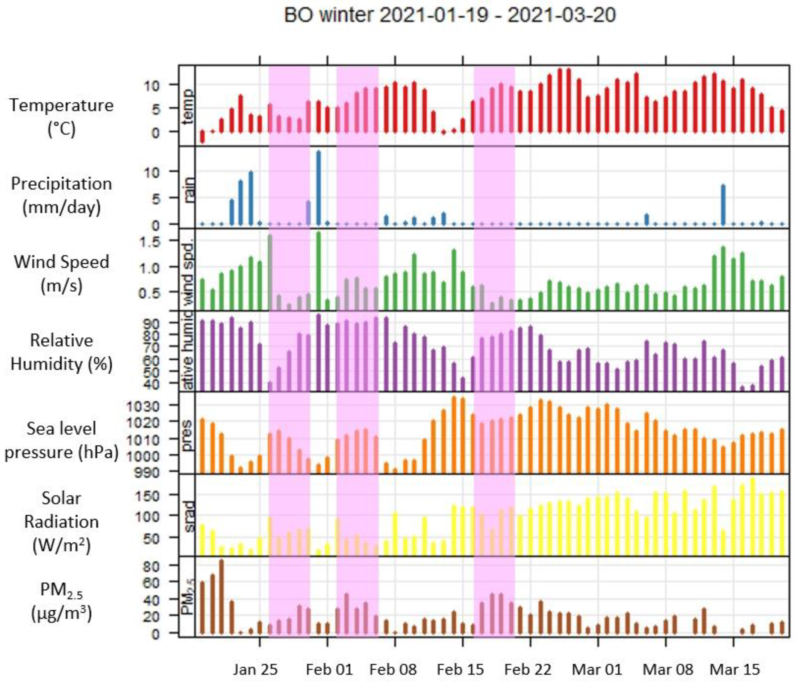
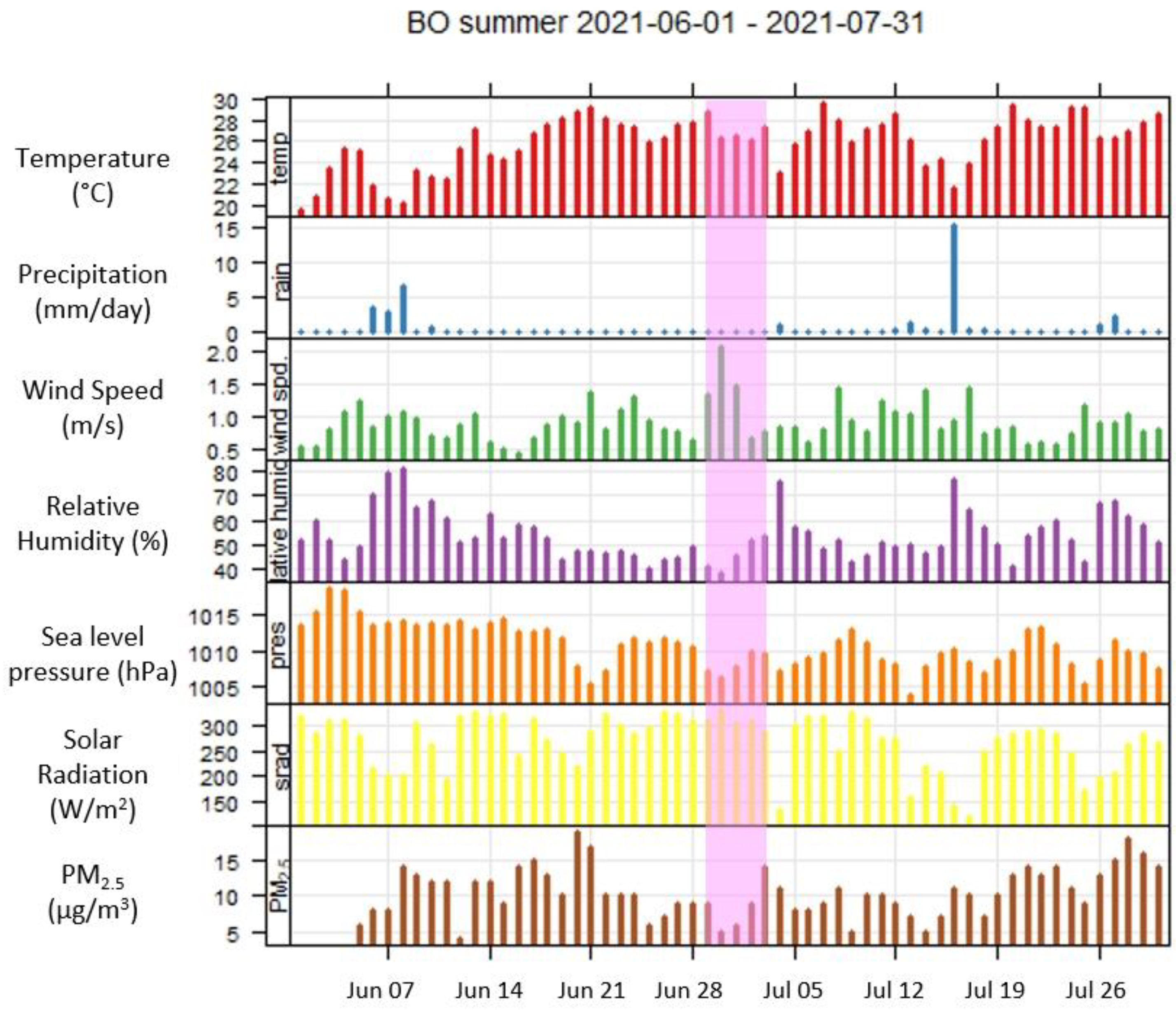
3.1. Meteorological Overview

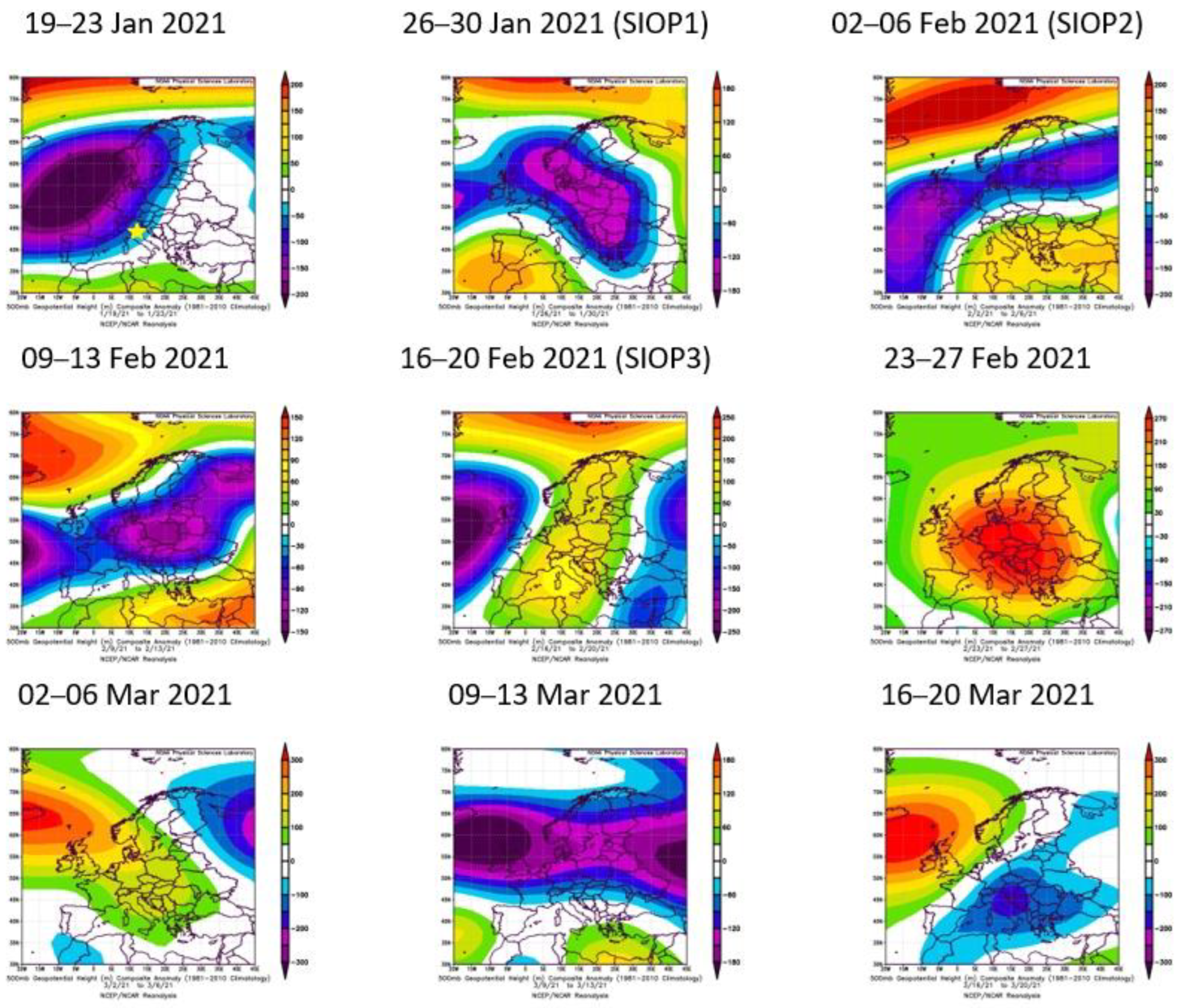
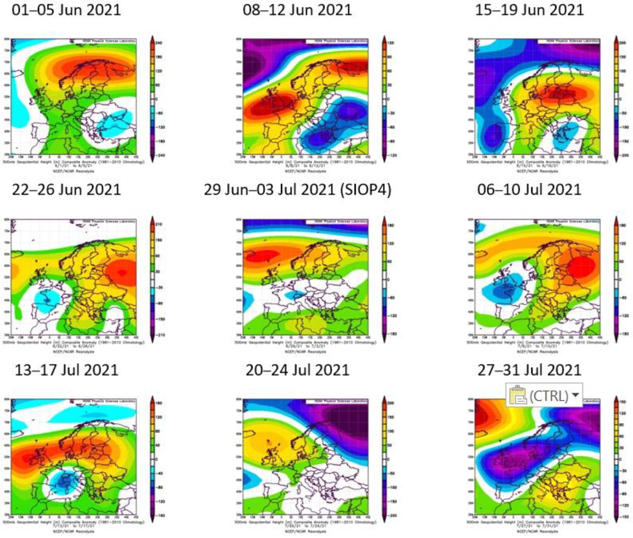
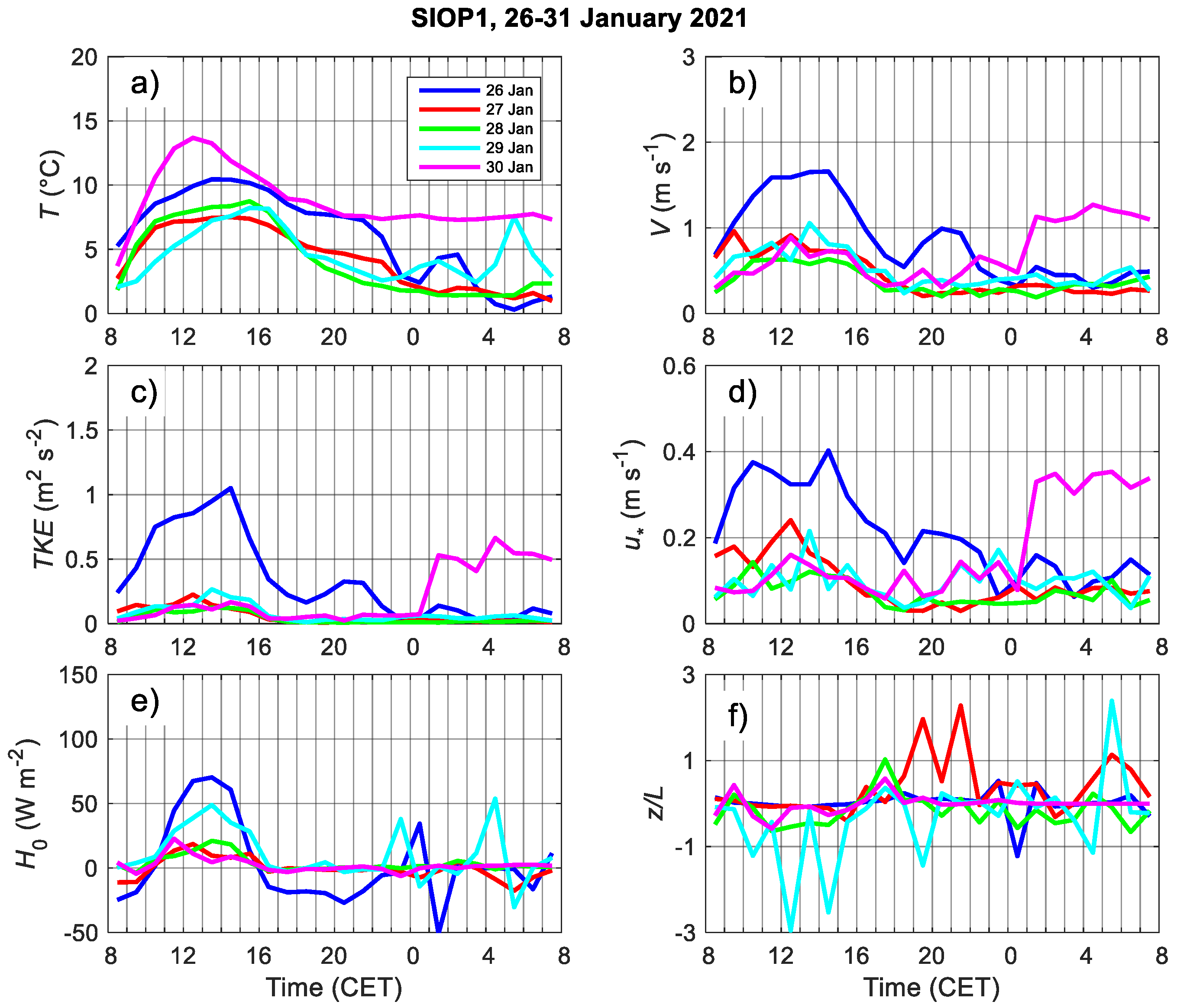
3.1.1. Meteorology of IOPs

To better describe the meteorology during the IOPs and SIOPs, it is convenient to organize the present brief meteorological analysis in weekly time slots, showing the Tuesday–Friday average synoptic conditions.

In Figure 2, we show the maps over Europe of the average geopotential height anomaly at 500 hPa with respect to the 1981–2010 mean from NCEP/NCAR Reanalysis during the winter campaign, and in Figure 3, the time series of main meteorological variables recorded in Bologna with the indication of the SIOPs.

In the Supplementary Materials (Figures S1 and S2) we show additional data of the winter campaign.

Starting from the second week (26–30 January), an anticyclonic ridge gradually mounted the western Mediterranean basin, initially determining sunnier and drier conditions. The first SIOP took place during this week. As the anticyclone expanded eastward (2–6 February, SIOP2), the arrival of warm southerly air masses over western Europe favored the formation of low clouds (and fog) with rising temperature and calm winds. A Saharan dust plume was also advected over the low-cloud deck by the end of the week (Figure S3). The PM_2.5 mass concentrations were generally higher than in the adjacent weeks during the two SIOP periods. In the following week (9–13 February), a cyclonic structure over central Europe pushed the anticyclone to the south, driving a more zonal flow with moderate winds, some light rain, a sharp temperature drop, and a decrease in PM_2.5 mass concentration.

From the subsequent week (16–20 February, SIOP3), an anticyclone settled over west-central Europe, bringing sunnier weather with increasing temperatures and light winds from the east. These conditions favored the accumulation of pollutants near the surface because of the reduced ventilation of the Po Valley, resulting in the highest PM_2.5 mass concentrations of the winter campaign (up to 50 μg m⁻³). The prevailing anticyclonic circulation persisted in the last week of February and 1 March, but with slightly enhanced ventilation in the Po Valley, which resulted in generally lower PM_2.5 concentrations with respect to the SIOP3 period. An incursion of Saharan dust also took place in the area, with a peak on 23 February (Figure S4). In the final period (9–20 March), low-pressure systems prevailed in central Europe, yielding a few rain episodes, stronger winds, and reduced PM_2.5 concentrations over the campaign location.

In Figure 4, we show the maps of geopotential height anomaly, and in Figure 5, the time series in Bologna for the summer campaign (June–July 2021). In the first week (1–5 June), the western Mediterranean was under the influence of the southern offshoots of a high-pressure system over northern Europe, which determined a relatively cold air flow from the north, resulting in mild temperatures and light winds in the campaign area. The following week (8–12 June), the anticyclone was pushed eastward by a reinforcing low-pressure system over south-eastern Europe, which brought clouds, rain, and a modest reduction of PM_2.5 mass concentration.

Afterward (15–26 June), a new anticyclone over central Europe took control of circulation over the Mediterranean basin, with south-easterly winds yielding high temperatures and dust advection from northern Africa toward Italy. The peak of the dust event (20–21 June) was well visible from satellite imagery (Figure S5) and was reflected in the highest PM_2.5 concentrations during the campaign.

In the week that we selected for the SIOP4 (29 June–3 July), the pressure field over southern Europe caused prevailing zonal winds that prevented the arrival of new dusty air masses, but also favored enhanced ventilation of the Po Valley, with a consequent relative reduction of PM_2.5 concentrations and synoptic-scale pressure until middle July then settled again into a pattern determining a prevailing flow from the south-east, with new dust advection in Italy (not shown). The second half of July was characterized by more variable weather, with a more frequent cloudy sky and few rain episodes, but with favorable conditions for the build-up of PM_2.5 concentrations.

The main motivation for the implementation of the operational forecast system was to provide information for the scheduling of the SIOPs, which had to be planned at least one week in advance. In the supplement, we include an assessment of the forecasting skills as a function of lead time (Figure S6).

3.1.2. Micrometeorology during the SIOPs

The time behavior of the temperature (a), wind speed (b), Turbulent Kinetic Energy (TKE) (c), friction velocity (d), H₀ (e), and z/L (f) during the four Super-Intensive Observational Periods, Winter SIOP1, SIOP2, SIOP3, and the summer SIOPS, are shown in Figure 6, Figure 7, Figure 8 and Figure 9 from 0800 CET of 1 day to 0800 CET of the following day. In the Supplementary (Figures S7–S14) we show variables measured during all the intensive observational periods.

For the sake of clarity, we note that the stability parameter z/L (f), representing the ratio of the sensor height above the ground (z) and the Monin–Obukhov length (L), might be informative of the atmospheric stratification: on land, the Obukhov length is positive (negative) for stable (unstable) stratification and becomes infinite in the limit of neutral stratification.

During SIOP1 (Figure 6), all the variables evidenced a similar behavior with a peak around 1300–1400 CET except for 30 January, which presented between 0000-0800 CET higher values of the temperature and the wind speed, and of all the variables related to mechanical mixing (u* and TKE). The larger values of the wind speed, sensible heat flux, and the variables related to the mechanical mixing were observed on 26 January. On this day, when sensible heat flux was negative, we observed values of TKE and U* larger than those of the other days of SIOP1. The mechanical mixing also had peaks during the afternoon until 0000 CET due to increasing wind speed values.

SIOP2 (Figure 7) is characterized by low values of the wind speed, TKE, u*, and temperature without a significant diurnal variation; this behavior is typical of cold and foggy days. The values of the sensible heat flux are below 50 W/m² except for 2 February, which evidences a weak diurnal behavior with characteristics similar to those of SIOP1.

During SIOP3 (Figure 8), all the variables show similar behavior with weak convection between 0800-1600 CET and peaking (all but temperature) between 1200–1400 CET. During SIOP4 (Figure 9), the registered values are those typical of summertime.

Maximum daily temperatures were between 30 °C and 35 °C; minimum temperatures were around 22 °C in the early morning. The diurnal behavior of temperature and H₀ was regular during all days. However, the wind regime in this period was variable and not regular. The first 3 days, 29 and 30 June, and 1 July, were characterized by moderate (for this site) wind speed between 2 and 3 m s⁻¹. On the next days, 2 and 3 July, very weak wind <1 m s⁻¹ occurred. The windiest day was 30 June. The values of u* and TKE followed the behavior of wind intensity. The values of the stability parameter z/L indicate the predominance of convective conditions between 0800 and 1600 CET. The occasional presence of unstable stratification also in the evening and nocturnal hours is probably due to the strong heating of the underlying surface covered with asphalt, which conserves higher temperatures during late hours.

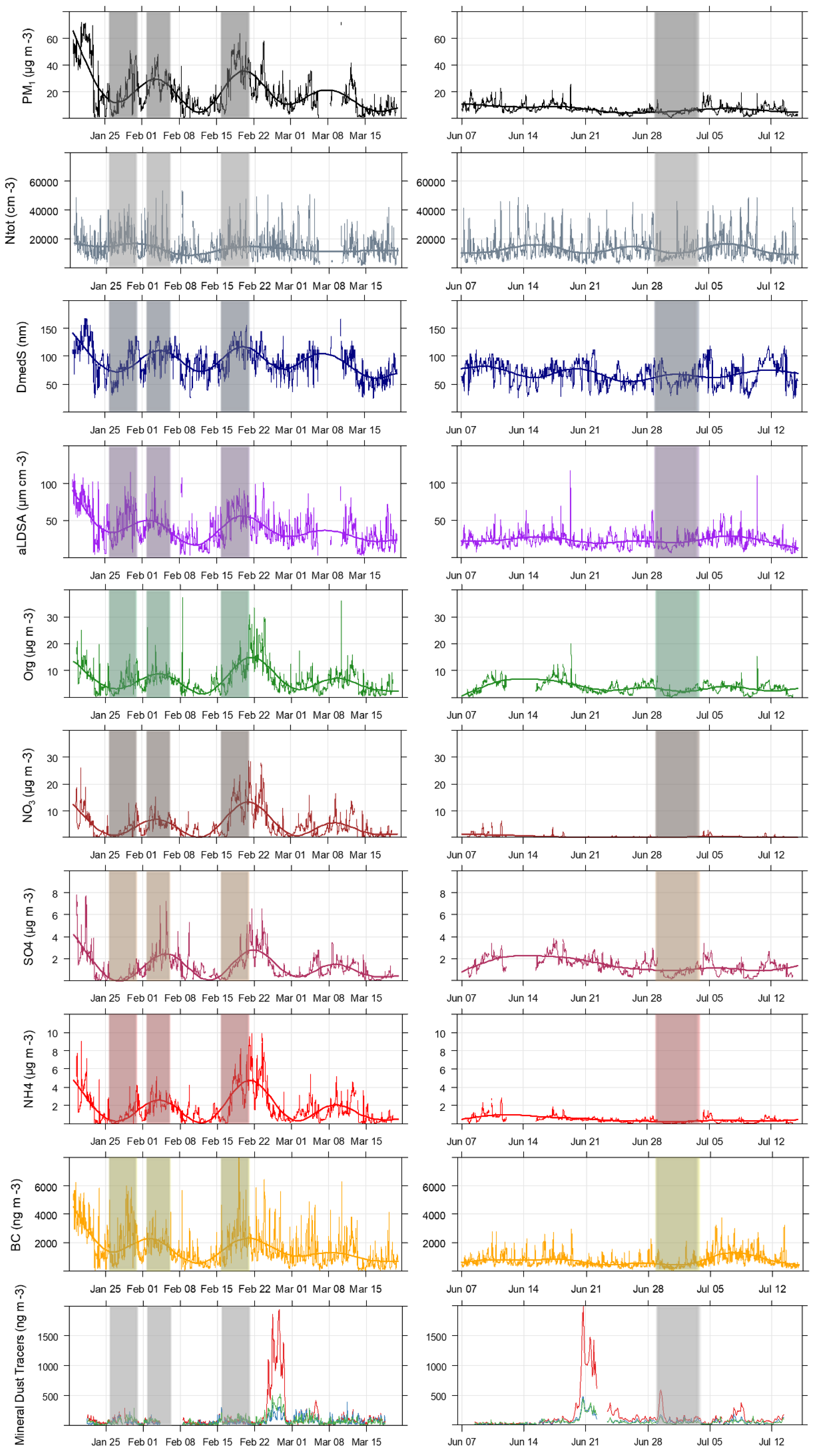
3.2. Atmospheric Aerosol Properties

Figure 10 shows the ranges of variability of PM₁ major components as measured at the urban site by the online equipment. We show first the mass concentration of PM₁, as reconstructed by SMPS data and validated on filter-based mass, after the procedure described in [11]. Then, PM₁ components, i.e., organic aerosol, nitrate, ammonium, sulfate, mineral dust tracers (e.g., Si, Ca, Fe, among others), and BC mass concentration are reported. The total number concentration is then represented, together with total surface area concentration and relevant aerosol size representative of the entire aerosol population (calculated as surface-weighted median mobility diameter [68]. Finally, we show the alveolar Lung Deposited Surface Area corresponding to the particle surface area size distribution weighted with the associated lung deposition curve and integrated over the whole particle size, the inhalation fraction according to the ICRP model [43].

Statistical data of commonly used aerosol metrics (PM₁, BC, LDSA, Particle number and size) are summarized in

Table 4. Descriptive Statistics of selected aerosol metrics: PM₁ (reconstructed from SMPS) and BC mass concentration, particle number (N_tot), alveolar Lung Deposited Surface Area (aLDSA), and particle median diameter (D_medS).

Metric		Winter (11 January 2021–31 March 2021)				Summer (27 May 2021–17 July 2021)
	UoM	Mean	Std.Dev.	Median	Range (Min–Max)	Mean	Std. Dev.	Median	Range (Min–Max)
PM1	μg/m3	20	15	16	0–76	7	3	6	1–26
Ntot	cm3	13,338	7441	11,928	1256–61,402	12,817	7776	10,586	2018–61,312
DmedS	nm	90	26	92	22–167	67	19	66	22–119
a-LDSA	μm2/cm3	39	22	35	2–146	23	9	21	5–117
BC	ng/m3	1496	1241	1163	6–32,275	677	456	551	33–8463

.

In the Supplementary Materials, we show statistics and data coverage of all the parameters measured at the urban site (Figure S15, Tables S4 and S5) and at the rural site of SPC (Figure S16). PAHs concentrations were measured at both sites during winter only, and they are reported in Figure S17 (in pg m⁻³).

It is worth mentioning that the sampling period—especially during the winter campaign—was characterized by a reduced anthropogenic activity due to COVID-19 pandemic restrictions. During wintertime, there were no relevant differences (i.e., in general, less than 20–25%) in average concentration values when comparing parallel samples collected at BO and SPC. PM₁ median mass concentration in winter was 19 ± 1 mg m₋₃ at both sites while, as expected, due to the stronger atmospheric dilution conditions, summertime PM₁ concentrations were approximately a factor 2 lower than wintertime ones. During wintertime, a large amount of the PM₁ median mass is accounted for by nitrate and organic carbon at both sites, and with comparable shares (18 and 22%, respectively), ammonium explains about 8% of the mass concentration, followed by sulfate (ca. 5%), elemental carbon and mineral dust (ca. 3–5% each), and heavy metal oxides (ca. 1%). In summer, the situation is quite different as the highest PM₁ mass share is related to organic carbon (29%), followed by sulfate (15%), mineral dust (12%), ammonium (7%), nitrate and elemental carbon (ca. 3–4% each) and heavy metal oxides (ca. 1%). In both seasons in BO and during the winter campaign at the SPC site, the average unaccounted mass (mainly related to the organic carbon to organic mass conversion factor and to undetected components like water) was in the range of 30–40%. As concerns PAHs concentrations at the urban background site, the most abundant species were benzo(b)fluoranthene and chrysene with average concentrations of 12 pg m^−3, followed by benzo(a)pyrene (7 pg m⁻³) and benz(a)anthracene (3 pg m⁻³); at the rural site concentration values were slightly lower with 10 and 9 pg m⁻³ for benzo(b)fluoranthene and chrysene, respectively, and 6 pg m⁻³ for benzo(a)pyrene and 2 pg m⁻³ for benz(a)anthracene

As a general feature, we note that particle mass (and surface area) concentrations and diameters were on average larger in winter than in summer. Mean PM₁ reconstructed from 5 min SMPS data and BC mass concentration ranged from 20 ± 15 μg m⁻³ to 7 ± 3 μg m⁻³ and from 1.5 ± 1.2 μg m⁻³ to 0.7 ± 0.5 μg m⁻³ in winter and summer, respectively, the mean surface-weighted diameters being 90 ± 26 nm in winter and 67 ± 19 nm in summer. Accordingly, a-LDSA was higher in winter (39 ± 22 μm²/cm³) than in summer (23 ± 9 μm²/cm³). Among PM₁ non-refractory components, all variables except sulfates (showing conversely similar values) were larger in winter than in summer. Like sulfates, total particle number concentration was on average similar in winter and summer, mean values being 1.3 × 10⁴ ± 0.7 × 10⁴ cm⁻³. Details on the particle number size distributions are provided in Figures S18 and S19.

These differences reflect different processes, dynamics, and sources governing the atmospheric aerosol in winter as compared to summer and the ability of the related metrics (i.e., number, mass, size of particles) to capture these. For example, in wintertime, higher combustion-related emission sources coupled to lower atmospheric mixing can result in higher particle mass—at least for BC. This is not necessarily the case for the total particle number, which is also significantly influenced by new particle formation (NPF) events. The smaller particle diameters in summer may likely be due to these different NPF rates in winter as compared to summer, coupled with the higher accumulation in the atmosphere (and hence particle aging) in winter. These topics will be analyzed in future publications. Here we note that these general features do reflect into the selected SIOPs. SIOP4 (30 June–3 July 2021), covering the summer period, shows the lowest concentrations of all variables except the particle number. Note an NPF event occurring during SIOP4 (on 2 July), but no NPF occurring during the winter SIOPs. Both SIOP1 (26–30 January 2021) and SIOP3 (16–20 February 2021) cover winter conditions with increasing concentrations and particle diameters (accumulation in the atmosphere). SIOP3 shows higher mass concentrations than SIOP1, which in turn shows higher number concentrations with smaller particle size. SIOP2 (2–6 February 2021) covers a period of stable concentrations with some foggy conditions.

3.3. Oxidative and Reducing Potential

Oxidative and reducing potentials of the 24 h PM₁ samples collected at BO and SPC during the winter and summer monitoring periods are summarized in

Table 5. Oxidative and reducing potentials of the 24 h PM₁ samples collected at BO and SPC during the winter and summer monitoring periods.

			OPDCFH	OPAA	OPDTT	OPDTTQRTZ	RPDPPH
		UoM	nmol H2O2 m−3	nmol AA min−1 m−3	nmol DTT min−1 m−3	nmol DTT min−1 m−3	% Cons DPPH m−3
		MDL	1.0 × 10−10	0.01	0.006	0.08	0.008
BO	Winter	Mean	4.7 × 10−9	0.37	0.91	0.58	0.42
		SD	3.1 × 10−9	0.35	0.55	0.25	0.42
		Median	4.1 × 10−9	0.27	0.83	0.53	0.33
		min–max	1.1 × 10−10–1.2 × 10−8	0.018–1.9	0.087–2.5	0.15–1.1	0.25–1.8
	Summer	Mean	1.6 × 10−9	0.47	0.31	0.22	0.045
		SD	1.4 × 10−9	0.54	0.17	0.10	0.087
		Median	1.5 × 10−9	0.23	0.31	0.22	0.046
		min–max	7.3 × 10−10–4.6 × 10−9	0.022–2.5	0.016–0.66	0.09–0.57	0.15–0.23
SPC	Winter	Mean	6.3 × 10−9	0.55	0.85	0.48	0.41
		SD	3.9 × 10−9	0.82	0.47	0.23	0.33
		Median	5.8 × 10−9	0.24	0.86	0.43	0.38
		min–max	1.9 × 10−10–1.6 × 10−8	0.010–4.6	0.006–2.0	0.22–1.2	0.11–1.3

.

From Table 5, we can observe that higher values of OP^DCFH and OP^DTT were measured at both sites in the colder period, characterized by less efficient mixing of air masses and greater accumulation of airborne pollutants. This shows that OP^DCFH and OP^DTT, as well as PM₁ concentration, were mainly modulated by seasonal atmospheric stability. In fact, OP^DCFH and OP^DTT are known to be predominantly sensitive to finer particles [69,70,71] that are more influenced by variations in atmospheric conditions and to domestic biomass heating [50,72,73], which is more intense during winter. The same can be pointed out for RP^DPPH; indeed, the reducing capacity of PM₁ seems to increase in winter, as well as for OP^DCFH and OP^DTT. Although not much is yet known about the PM reducing activity, these results highlighted the ability of RP^DPPH to predict PM₁ reducing properties.

The need to estimate the reducing potential of PM is related to the stability of the PM species: short-life oxidant species can react, and redox equilibria among PM native species could occur during both the sample storage and the extraction phase. In this regard, it is possible that, within the conditions that could contribute to the estimation of the oxidative potential of PM, there is also the reaction and/or competition between oxidant and reducing species naturally occurring in PM. Some studies proved the presence of species with likely reducing characteristics [74,75]. Although the nature of reducing species is still unknown, some studies proved the presence of species with likely antioxidant and reducing characteristics such as phenols from wood-burning or phenolic compounds from different sources. Furthermore, experimental OP values suggested the possible presence of this kind of species in PM and illustrated the need to deepen knowledge of the redox properties of PM. The estimation of reducing potential is aimed at clarifying the latter aspects by considering the application of an acellular procedure to evaluate the presence of reducing species in PM samples, along with the evaluation of the OP of PM. Therefore, the DPPH radical scavenging assay was adapted and applied to PM in order to verify its possible use as an acellular method for estimating the presence of reducing species, thus expressing PM reducing potential [48]. Preliminary applications of the DPPH assay revealed the presence of reducing species in several components of atmospheric PM derived from various emission sources and, thus, with very different chemical compositions [48]. This assay offers the advantages of being simple, rapid, and easily applicable to intensive PM monitoring campaigns for routinely estimating the amount of reducing species in PM samples. For what was mentioned above, the DPPH assay was applied during the RHAPS project to acquire new insights into the field of PM redox properties and their impacts on health outcomes and endpoints.

All these assays seem to be less affected by inter-site variability. On the contrary, OP^AA appears to be less modulated by seasonal variations and more influenced by different contributions of the emission sources at the two sites. The daily contribution of the different emission sources to the oxidative and reducing capacity of PM₁ and the associated toxicological potential will be extensively evaluated in future studies.

3.4. Toxicological Assessment

3.4.1. Effects of PM₁ from Water-Extracted Samples during IOPs

Effects of PM₁ from water-extracted filter samples were investigated in BEAS-2B cells as a surrogate of epithelial lung cells and THP-1 cells as a surrogate of alveolar macrophages. For illustrative purposes, the results of IL-8 release in both cell types are reported in Figure 11.

Results are expressed as % of control. In THP-1 cells, seasonal and site differences were observed in average responses, with higher releases observed in SPC compared to BO and higher production in summer vs. winter samples obtained in BO. In addition, daily differences in IL-8 release were also observed. Regarding the release of IL-8 in BEAS-2B cells, no seasonal or site differences in the average responses were found. In the majority of the samples, the release of IL-8 was above control values. These results confirm the ability of the models used to respond to PM₁ water-extracted filters, with a different sensitivity between the two models and in relation to specific components.

Embryotoxicity tests were also performed on the same water extracted samples. Indeed, an embryo represents a complex biological model responding to environmental signals blocking, changing the speed of development, or altering the normal morphogenetical pattern. Preliminary results show that neither lethal nor malformative effects were recorded after the exposure to the water extract fraction (Figure S20).

3.4.2. Effects in Cells Exposed at the Air Liquid Interface during SIOPs

The average responses in exposed cells show a non-significant difference between winter and summer campaigns except for a significant difference in Cxcl-8 gene expression (p = 0.04, ANOVA, Analysis of Variance) and IL-8 release (p = 0.02, ANOVA) that were higher in winter samples (Figure 12). A slight but not significant increase in winter samples is also reported for NQO1 and HMOX genes. However, differences among the different days of exposure are evident for the scatterplot properties, and this distribution of the responses may indicate an altered gene expression in relation to specific aerosol properties.

4. Discussion and Conclusions

Linking air quality and health is still a complex issue. The debate on which particle type is more or less toxic [76] and how to protect human health [3,77] is still unresolved. In the meantime, the last WHO guidelines [1] (WHO 2021) tend to reduce as much as possible the thresholds of safety for human health, suggesting the absence of a safe threshold for PM_2.5. To target this topic, the RHAPS experiment aims to identify specific properties of PM₁ from combustion sources that are responsible for toxicological effects and can be used as new metrics for health-related outdoor pollution studies. In this paper, we present the overall methodology of the RHAPS project and introduce the phenomenology and the first data observed.

The first results show that at real atmospheric conditions (i.e., PM₁ of about 20 μg m⁻³):

• high values of PM₁ mass concentration do not necessarily translate into high toxicity (i.e., PM₁ mass concentration > 50 μg m⁻³ ), and conversely, very low values of PM₁ (mass concentration < 5 μg m⁻³ ) do not necessarily translate into no toxicity;
• high values of BC mass concentration do not necessarily translate into high toxicity (BC mass concentration > 5 μg m⁻³);
• different WSOP assays may give different responses, but in general, high values of WSOP do not necessarily translate into high toxicity.

Notably, these findings were observed during a variety of atmospheric conditions, aerosol properties, and toxicological assessments.

Regarding the atmospheric conditions, in winter (temperature ranging from −5 to 15 °C), we observed sunnier and drier conditions (SIOP1), low-clouds (and fog) with rising temperature and calm winds (SIOP2), Saharan dust plumes with high PM_2.5, and accumulation of pollutants near the surface with the highest PM_2.5 mass concentrations of the winter campaign (up to 50 μg m⁻³, SIOP3). In summer (temperatures from 0 to 35 °C), we had light winds, clouds, rain, and a modest reduction of PM_2.5 mass concentration, dust advection with high PM_2.5, enhanced ventilation, with a consequent relative reduction of PM_2.5 concentrations (SIOP4).

Regarding aerosol properties, overall, our data are representative of PM₁ concentration from 0 to 60 μg m⁻³, BC from 0 to 6 μg m^−3, and particle number from 0 to 6.0 × 10⁵ cm⁻³. During wintertime, aerosol particle mass was higher. PM₁ mass concentration was, on average, approx. 20 μg m⁻³ at both the rural and urban sites, and it was mainly accounted for by secondary inorganic ions (i.e., sulfate, nitrate, and ammonium) together with organic carbon. In summer, PM₁ concentrations were approximately a factor 2 lower than wintertime ones, and the major components were sulfates and OC. All PM₁ components (BC, OA, nitrates, and ammonium) except sulfates were larger in winter than in summer. Contrarily to most of the PM₁ mass components except sulfates, the total particle number concentration was on average similar in winter and summer (on average, 1.3 × 10⁴ cm⁻³), particle size being smaller in summer (surface-weighted diameter approx. 65 nm in summer, and 90 nm in winter).

Considering WSOP, both OP^DCFH and OP^DTT were higher at both sites in winter than in summer. Also, the reducing capacity of PM₁ (RP^DPPH) seems to increase in winter. Conversely, OP^AA is slightly higher (or comparable) in summer than in winter.

These trends (e.g., higher PM₁ and BC and/or higher WSOP in winter) do not necessarily reflect the biological responses. Considering the water-extracted samples (“classical approach”) during the whole IOPs, we observed IL-8 releases higher in summer than in winter in THP-1 cells, and no seasonal difference in BEAS-2B cells (the majority of the samples having the release of IL-8 above control values). Considering the cells exposed at the Air Liquid Interface directly in the atmosphere (“the original approach” that we developed) during the SIOPs, we observed no significant difference on average between winter and summer for most of the genes analyzed, except for a significant difference in Cxcl-8 gene expression and IL-8 release that were higher in winter. Note that the summer SIOP4 had very low mass concentrations (PM₁ < 5 mg m⁻³).

Differences among the different days of exposure are conversely evident.

Therefore, the first findings suggest that high/low PM₁ and BC mass concentration and WSOP do not necessarily translate into high/low toxicity but that the complexity of biological responses might go beyond these. These preliminary findings will be discussed in detail in a series of companion papers, with a focus basically on four topics:

• Source apportionment of PM₁ and the role of source emissions on aerosol toxicity;
• OP as a predictive variable for PM₁ toxicity with a focus on SOA possessing redox-active capacity;
• Exposure-response relationships for PM₁;
• Air quality models to forecast PM₁ toxicity.

The hypothesis to test is that the exposure to primary and secondary atmospheric aerosols under conditions representative of the real-life scenario in the atmosphere can differently activate oxidative stress and inflammatory responses. It is worth noting that the real-life scenario is a major focus of the RHAPS project, where exposure is assessed to the real atmospheric concentrations, as pioneeringly proposed during the first CARE experiment [11]. Future papers (manuscripts in preparation) will investigate this by analyzing physicochemical properties and specific metrics (both classical and newly developed) of source-specific primary and secondary aerosol, and exploring connections between all these metrics and the release of biological markers in lung epithelial cells, the focus on oxidative stress-related pathways. Importantly, beyond PM₁ and BC mass concentration, we will include among these metrics the source-apportioned PM₁ oxidative potential and statistical profiles of source-specific aerosol types such as SOA. The assessment of the redox-active capacity of SOA will be derived from the comprehensive RHAPS assessment from in-field and laboratory measurements. Anthropogenic aerosol secondary organic compounds, such as quinones, are considered among the most important players in determining OP [78] and are known to generate from photochemical aging of the emissions of a very broad range of combustion systems [6]. The variability in aerosol properties and in OP will be specifically linked to changes in distinct source contributions with the novel source apportionment approach of RHAPS by inserting each data value in its original time schedule through advanced receptor modeling [79,80,81,82]. The insertion of non-compositional variables (e.g., absorption coefficients or OP) in the same modeling process, the combination with fossil fuel and biomass burning EC and OC components from optical source apportionment as well as the organic aerosol components retrieved from the AMS apportionment will be key for robust source identification and assessment. As the final step, the air quality modeling will be devoted to developing an operational air quality forecast tool for PM toxicity to be deployed on a national scale. Findings will be among the first results of this kind and have the potential to support the development of new metrics for health-related pollution studies and contribute to the cutting-edge research on OP and SOA.

References

1. World Health Organization; WHO European Centre for Environment. WHO Global Air Quality Guidelines: Particulate Matter (PM2.5 and PM10), Ozone, Nitrogen Dioxide, Sulfur Dioxide and Carbon Monoxide; World Health Organization: Geneva, Switzerland, 2021.
2. Chen, J.; Hoek, G. Long-term exposure to PM and all-cause and cause-specific mortality: A systematic review and meta-analysis. Environ. Int. 2020, 143, 105974. [Google Scholar] [CrossRef] [PubMed]
3. Stafoggia, M.; Oftedal, B.; Chen, J.; Rodopoulou, S.; Renzi, M.; Atkinson, R.W.; Janssen, N.A. Long-term exposure to low ambient air pollution concentrations and mortality among 28 million people: Results from seven large European cohorts within the ELAPSE project. Lancet Planet. Health 2022, 6, e9–e18. [Google Scholar] [CrossRef]
4. Li, X.; Jin, L.; Kan, H. Air pollution: A global problem needs local fixes. Nature 2019, 570, 437–439. [Google Scholar] [CrossRef] [PubMed] [Green Version]
5. Künzi, L.; Krapf, M.; Daher, N.; Dommen, J.; Jeannet, N.; Schneider, S.; Geiser, M. Toxicity of aged gasoline exhaust particles to normal and diseased airway epithelia. Sci. Rep. 2015, 5, 11801. [Google Scholar] [CrossRef] [PubMed] [Green Version]
6. Jimenez, J.L.; Canagaratna, M.R.; Donahue, N.M.; Prevot, A.S.H.; Zhang, Q.; Kroll, J.H.; Worsnop, D.R. Evolution of organic aerosols in the atmosphere. Science 2009, 326, 1525–1529. [Google Scholar] [CrossRef] [PubMed]
7. Ervens, B.T.B.W.R.; Turpin, B.J.; Weber, R.J. Secondary organic aerosol formation in cloud droplets and aqueous particles (aqSOA): A review of laboratory, field and model studies. Atmos. Chem. Phys. 2011, 11, 11069–11102. [Google Scholar] [CrossRef] [Green Version]
8. Corsini, E.; Ozgen, S.; Papale, A.; Galbiati, V.; Lonati, G.; Fermo, P.; Marinovich, M. Insights on wood combustion generated proinflammatory ultrafine particles (UFP). Toxicol. Lett. 2017, 266, 74–84. [Google Scholar] [CrossRef]
9. Corsini, E.; Vecchi, R.; Marabini, L.; Fermo, P.; Becagli, S.; Bernardoni, V.; Marinovich, M. The chemical composition of ultrafine particles and associated biological effects at an alpine town impacted by wood burning. Sci. Total Environ. 2017, 587, 223–231. [Google Scholar] [CrossRef]
10. Marabini, L.; Ozgen, S.; Turacchi, S.; Aminti, S.; Arnaboldi, F.; Lonati, G.; Marinovich, M. Ultrafine particles (UFPs) from domestic wood stoves: Genotoxicity in human lung carcinoma A549 cells. Mutat. Res. Genet. Toxicol. Environ. Mutagenesis 2017, 820, 39–46. [Google Scholar] [CrossRef]
11. Costabile, F.; Alas, H.; Aufderheide, M.; Avino, P.; Amato, F.; Argentini, S.; Gobbi, G.P. First results of the “Carbonaceous aerosol in Rome and Environs (CARE)” experiment: Beyond current standards for PM10. Atmosphere 2017, 8, 249. [Google Scholar] [CrossRef] [Green Version]
12. Gualtieri, M.; Grollino, M.G.; Consales, C.; Costabile, F.; Manigrasso, M.; Avino, P.; Zanini, G. Is it the time to study air pollution effects under environmental conditions? A case study to support the shift of in vitro toxicology from the bench to the field. Chemosphere 2018, 207, 552–564. [Google Scholar] [CrossRef] [PubMed]
13. Kelly, F.J.; Fussell, J.C. Size, source and chemical composition as determinants of toxicity attributable to ambient particulate matter. Atmos. Environ. 2012, 60, 504–526. [Google Scholar] [CrossRef]
14. Lakey, P.S.; Berkemeier, T.; Tong, H.; Arangio, A.M.; Lucas, K.; Pöschl, U.; Shiraiwa, M. Chemical exposure-response relationship between air pollutants and reactive oxygen species in the human respiratory tract. Sci. Rep. 2016, 6, 32916. [Google Scholar] [CrossRef]
15. Saffari, A.; Daher, N.; Shafer, M.M.; Schauer, J.J.; Sioutas, C. Global perspective on the oxidative potential of airborne particulate matter: A synthesis of research findings. Environ. Sci. Technol. 2014, 48, 7576–7583. [Google Scholar] [CrossRef] [PubMed]
16. Decesari, S.; Sowlat, M.H.; Hasheminassab, S.; Sandrini, S.; Gilardoni, S.; Facchini, M.C.; Sioutas, C. Enhanced toxicity of aerosol in fog conditions in the Po Valley, Italy. Atmos. Chem. Phys. 2017, 17, 7721–7731. [Google Scholar] [CrossRef] [Green Version]
17. Verma, V.; Fang, T.; Xu, L.; Peltier, R.E.; Russell, A.G.; Ng, N.L.; Weber, R.J. Organic aerosols associated with the generation of reactive oxygen species (ROS) by water-soluble PM2.5. Environ. Sci. Technol. 2015, 49, 4646–4656. [Google Scholar] [CrossRef]
18. Janssen, N.A.; Yang, A.; Strak, M.; Steenhof, M.; Hellack, B.; Gerlofs-Nijland, M.E.; Cassee, F. Oxidative potential of particulate matter collected at sites with different source characteristics. Sci. Total Environ. 2014, 472, 572–581. [Google Scholar] [CrossRef] [Green Version]
19. Sarti, E.; Pasti, L.; Rossi, M.; Ascanelli, M.; PAgnoni, A.; Trombini, M.; Remelli, M. The composition of PM1 and PM2.5 samples, metals and their water soluble fractions in the Bologna area (Italy). Atmos. Pollut. Res. 2015, 6, 708–718. [Google Scholar] [CrossRef] [Green Version]
20. Vecchi, R.; Marcazzan, G.; Valli, G.; Ceriani, M.; Antoniazzi, C. The role of atmospheric dispersion in the seasonal variation of PM1 and PM2.5 concentration and composition in the urban area of Milan (Italy). Atmos. Environ. 2004, 38, 4437–4446. [Google Scholar] [CrossRef]
21. Amato, F.; Alastuey, A.; Karanasiou, A.; Lucarelli, F.; Nava, S.; Calzolai, G.; Querol, X. AIRUSE-LIFE+: A harmonized PM speciation and source apportionment in five southern European cities. Atmos. Chem. Phys. 2016, 16, 3289–3309. [Google Scholar] [CrossRef] [Green Version]
22. Ricciardelli, I.; Bacco, D.; Rinaldi, M.; Bonafè, G.; Scotto, F.; Trentini, A.; Poluzzi, V. A three-year investigation of daily PM2.5 main chemical components in four sites: The routine measurement program of the Supersito Project (Po Valley, Italy). Atmos. Environ. 2017, 152, 418–430. [Google Scholar] [CrossRef]
23. Gilardoni, S.; Massoli, P.; Paglione, M.; Giulianelli, L.; Carbone, C.; Rinaldi, M.; Facchini, M.C. Direct observation of aqueous secondary organic aerosol from biomass-burning emissions. Proc. Natl. Acad. Sci. USA 2016, 113, 10013–10018. [Google Scholar] [CrossRef] [Green Version]
24. Lucarelli, F.; Calzolai, G.; Chiari, M.; Giardi, F.; Czelusniak, C.; Nava, S. Hourly elemental composition and source identification by Positive Matrix Factorization (PMF) of fine and coarse particulate matter in the high polluted industrial area of Taranto (Italy). Atmosphere 2020, 11, 419. [Google Scholar] [CrossRef] [Green Version]
25. Massimi, L.; Ristorini, M.; Astolfi, M.L.; Perrino, C.; Canepari, S. High resolution spatial mapping of element concentrations in PM10: A powerful tool for localization of emission sources. Atmos. Res. 2020, 244, 105060. [Google Scholar] [CrossRef]
26. Astolfi, M.L.; Protano, C.; Marconi, E.; Massimi, L.; Brunori, M.; Piamonti, D.; Canepari, S. A new rapid treatment of human hair for elemental determination by inductively coupled mass spectrometry. Anal. Methods 2020, 12, 1906–1918. [Google Scholar] [CrossRef]
27. Canepari, S.; Pietrodangelo, A.; Perrino, C.; Astolfi, M.L.; Marzo, M.L. Enhancement of source traceability of atmospheric PM by elemental chemical fractionation. Atmos. Environ. 2009, 43, 4754–4765. [Google Scholar] [CrossRef]
28. Piazzalunga, A.; Bernardoni, V.; Fermo, P.; Vecchi, R. Optimisation of analytical procedures for the quantification of ionic and carbonaceous fractions in the atmospheric aerosol and applications to ambient samples. Anal. Bioanal. Chem. 2013, 405, 1123–1132. [Google Scholar] [CrossRef]
29. Piazzalunga, A.; Fermo, P.; Bernardoni, V.; Vecchi, R.; Valli, G.; de Gregorio, M.A. A simplified method for levoglucosan quantification in wintertime atmospheric particulate matter by high performance anion-exchange chromatography coupled with pulsed amperometric detection. Int. J. Environ. Anal. Chem. 2010, 90, 934–947. [Google Scholar] [CrossRef] [Green Version]
30. Terzopoulou, E.; Voutsa, D.; Kaklamanos, G. A multi-residue method for determination of 70 organic micropollutants in surface waters by solid-phase extraction followed by gas chromatography coupled to tandem mass spectrometry. Environ. Sci. Pollut. Res. 2015, 22, 1095–1112. [Google Scholar] [CrossRef]
31. Gosetti, F.; Chiuminatto, U.; Mazzucco, E.; Robotti, E.; Calabrese, G.; Gennaro, M.C.; Marengo, E. Simultaneous determination of thirteen polycyclic aromatic hydrocarbons and twelve aldehydes in cooked food by an automated on-line solid phase extraction ultra high performance liquid chromatography tandem mass spectrometry. J. Chromatogr. A 2011, 1218, 6308–6318. [Google Scholar] [CrossRef]
32. Canagaratna, M.R.; Jayne, J.T.; Jimenez, J.L.; Allan, J.D.; Alfarra, M.R.; Zhang, Q.; Worsnop, D.R. Chemical and microphysical characterization of ambient aerosols with the aerodyne aerosol mass spectrometer. Mass Spectrom. Rev. 2007, 26, 185–222. [Google Scholar] [CrossRef]
33. Jayne, J.T.; Leard, D.C.; Zhang, X.; Davidovits, P.; Smith, K.A.; Kolb, C.E.; Worsnop, D.R. Development of an aerosol mass spectrometer for size and composition analysis of submicron particles. Aerosol Sci. Technol. 2000, 33, 49–70. [Google Scholar] [CrossRef] [Green Version]
34. Jimenez, J.L.; Jayne, J.T.; Shi, Q.; Kolb, C.E.; Worsnop, D.R.; Yourshaw, I.; Davidovits, P. Ambient aerosol sampling using the aerodyne aerosol mass spectrometer. J. Geophys. Res. Atmos. 2003, 108, 8425. [Google Scholar] [CrossRef] [Green Version]
35. DeCarlo, P.F.; Kimmel, J.R.; Trimborn, A.; Northway, M.J.; Jayne, J.T.; Aiken, A.C.; Jimenez, J.L. Field-deployable, high-resolution, time-of-flight aerosol mass spectrometer. Anal. Chem. 2006, 78, 8281–8289. [Google Scholar] [CrossRef]
36. Middlebrook, A.M.; Bahreini, R.; Jimenez, J.L.; Canagaratna, M.R. Evaluation of composition-dependent collection efficiencies for the aerodyne aerosol mass spectrometer using field data. Aerosol Sci. Technol. 2012, 46, 258–271. [Google Scholar] [CrossRef]
37. Calzolai, G.; Lucarelli, F.; Chiari, M.; Nava, S.; Giannoni, M.; Carrarese, L.; Prati, P.; Vecchi, R. Improvements in PIXE analysis of hourly particulate matter samples. Nucl. Instrum. Methods Phys. Res. B 2015, 363, 99–104. [Google Scholar] [CrossRef]
38. Hinds, W.C. Aerosol Technology: Properties, Behavior and Measurement of Airborne Particles, 2nd ed.; John Wiley & Sons: New York, NY, USA, 1999. [Google Scholar]
39. Massabò, D.; Bernardoni, V.; Bove, M.C.; Brunengo, A.; Cuccia, E.; Piazzalunga, A.; Vecchi, R. A multi-wavelength optical set-up for the characterization of carbonaceous particulate matter. J. Aerosol Sci. 2013, 60, 34–46. [Google Scholar] [CrossRef]
40. Massabò, D.; Caponi, L.; Bernardoni, V.; Bove, M.C.; Brotto, P.; Calzolai, G.; Prati, P. Multi-wavelength optical determination of black and brown carbon in atmospheric aerosols. Atmos. Environ. 2015, 108, 1–12. [Google Scholar] [CrossRef]
41. Moosmüller, H.; Chakrabarty, R.K.; Ehlers, K.M.; Arnott, W.P. Absorption Ångström coefficient, brown carbon, and aerosols: Basic concepts, bulk matter, and spherical particles. Atmos. Chem. Phys. 2011, 11, 1217–1225. [Google Scholar] [CrossRef] [Green Version]
42. Sandradewi, J.; Prévôt, A.S.; Szidat, S.; Perron, N.; Alfarra, M.R.; Lanz, V.A.; Baltensperger, U.R.S. Using aerosol light absorption measurements for the quantitative determination of wood burning and traffic emission contributions to particulate matter. Environ. Sci. Technol. 2008, 42, 3316–3323. [Google Scholar] [CrossRef]
43. Bernardoni, V.; Pileci, R.E.; Caponi, L.; Massabò, D. The Multi-Wavelength Absorption Analyzer (MWAA) Model as a Tool for Source and Component Apportionment Based on Aerosol Absorption Properties: Application to Samples Collected in Different Environments. Atmosphere 2017, 8, 218. [Google Scholar] [CrossRef] [Green Version]
44. Massabò, D.; Altomari, A.; Vernocchi, V.; Prati, P. Two-wavelength thermal–optical determination of light-absorbing carbon in atmospheric aerosols. Atmos. Meas. Tech. 2019, 12, 3173–3182. [Google Scholar] [CrossRef] [Green Version]
45. Massabò, D.; Prati, P.; Canepa, E.; Bastianini, M.; van Eijk, A.M.; Missamou, T.; Piazzola, J. Characterization of carbonaceous aerosols over the Northern Adriatic Sea in the JERICO-NEXT project framework. Atmos. Environ. 2020, 228, 117449. [Google Scholar] [CrossRef]
46. Drinovec, L.; Močnik, G.; Zotter, P.; Prévôt, A.S.H.; Ruckstuhl, C.; Coz, E.; Hansen, A.D.A. The “dual-spot” Aethalometer: An improved measurement of aerosol black carbon with real-time loading compensation. Atmos. Meas. Tech. 2015, 8, 1965–1979. [Google Scholar] [CrossRef] [Green Version]
47. National Institute for Occupational Safety and Health. NIOSH: Method 5040 Issue 3: Elemental Carbon (Diesel Exhaust). In NIOSH Manual of Analytical Methods; National Institute of Occupational Safety and Health: Cincinnati, OH, USA, 1999. [Google Scholar]
48. Frezzini, M.A.; Castellani, F.; de Francesco, N.; Ristorini, M.; Canepari, S. Application of DPPH assay for assessment of particulate matter reducing properties. Atmosphere 2019, 10, 816. [Google Scholar] [CrossRef] [Green Version]
49. Frezzini, M.A.; de Francesco, N.; Massimi, L.; Canepari, S. Effects of operating conditions on PM oxidative potential assays. Atmos. Environ. 2021, 268, 118802. [Google Scholar] [CrossRef]
50. Massimi, L.; Ristorini, M.; Simonetti, G.; Frezzini, M.A.; Astolfi, M.L.; Canepari, S. Spatial Mapping and Size Distribution of Oxidative Potential of Particulate Matter Released by Spatially Disaggregated Sources. Environ. Pollut. 2020, 266, 115271. [Google Scholar] [CrossRef]
51. Kedare, S.B.; Singh, R.P. Genesis and development of DPPH method of antioxidant assay. J. Food Sci. Technol. 2011, 48, 412–422. [Google Scholar] [CrossRef] [Green Version]
52. Hara, K.; Someya, T.; Sano, K.; Sagane, Y.; Watanabe, T.; Wijesekara, R.G.S. Antioxidant activities of traditional plants in Sri Lanka by DPPH free radical-scavenging assay. Data Brief 2018, 17, 870–875. [Google Scholar] [CrossRef]
53. Chedea, V.S.; Pop, R.M. Total polyphenols content and antioxidant DPPH assays on biological samples. In Polyphenols in Plants; Academic Press: Cambridge, MA, USA, 2019; pp. 169–183. [Google Scholar]
54. Sridhar, K.; Charles, A.L. In vitro antioxidant activity of Kyoho grape extracts in DPPH and ABTS assays: Estimation methods for EC50 using advanced statistical programs. Food Chem. 2019, 275, 41–49. [Google Scholar] [CrossRef]
55. Cho, A.K.; Sioutas, C.; Miguel, A.H.; Kumagai, Y.; Schmitz, D.A.; Singh, M.; Froines, J.R. Redox activity of airborne particulate matter at different sites in the Los Angeles Basin. Environ. Res. 2005, 99, 40–47. [Google Scholar] [CrossRef] [PubMed]
56. Verma, V.; Ning, Z.; Cho, A.K.; Schauer, J.J.; Shafer, M.M.; Sioutas, C. Redox activity of urban quasi-ultrafine particles from primary and secondary sources. Atmos. Environ. 2009, 43, 6360–6368. [Google Scholar] [CrossRef]
57. Gao, D.; Fang, T.; Verma, V.; Zeng, L.; Weber, R.J. A method for measuring total aerosol oxidative potential (OP) with the dithiothreitol (DTT) assay and comparisons between an urban and roadside site of water-soluble and total OP. Atmos. Meas. Tech. 2017, 10, 2821–2835. [Google Scholar] [CrossRef] [Green Version]
58. Simonetti, G.; Frasca, D.; Marcoccia, M.; Farao, C.; Canepari, S. Multi-elemental analysis of particulate matter samples collected by a particle-into-liquid sampler. Atmos. Pollut. Res. 2018, 9, 747–754. [Google Scholar] [CrossRef]
59. Costabile, F.; Gualtieri, M.; Canepari, S.; Tranfo, G.; Consales, C.; Grollino, M.G.; Simonetti, G. Evidence of association between aerosol properties and in-vitro cellular oxidative response to PM1, oxidative potential of PM2.5, a biomarker of RNA oxidation, and its dependency on combustion sources. Atmos. Environ. 2019, 213, 444–455. [Google Scholar] [CrossRef]
60. Corsini, E.; Budello, S.; Marabini, L.; Galbiati, V.; Piazzalunga, A.; Barbieri, P.; Galli, C.L. Comparison of wood smoke PM2.5 obtained from the combustion of FIR and beech pellets on inflammation and DNA damage in A549 and THP-1 human cell lines. Arch. Toxicol. 2013, 87, 2187–2199. [Google Scholar] [CrossRef]
61. Battistoni, M.; Bacchetta, R.; Di Renzo, F.; Metruccio, F.; Moretto, A.; Menegola, E. Modified Xenopus laevis approach (R-FETAX) as an alternative test for the evaluation of foetal valproate spectrum disorder. Reprod. Toxicol. 2022, 107, 140–149. [Google Scholar] [CrossRef]
62. Brown, N.A.; Fabro, S. Quantitation of rat embryonic development in vitro: A morphological scoring system. Teratology 1981, 24, 65–78. [Google Scholar] [CrossRef] [PubMed]
63. Nieuwkoop, P.D.; Faber, J.; Gerhart, J.; Kirschner, M. Normal Table of Xenopus laevis (Daudin): A Systematical and Chronological Survey of the Development From the Fertilized Egg till the End of Metamorphosis; Garland Science: New York, NY, USA, 2020. [Google Scholar]
64. Skamarock, W.C.; Klemp, J.B.; Dudhia, J.; Gill, D.O.; Barker, D.M.; Wang, W.; Powers, J.G. A Description of the Advanced Research WRF Version 2; National Center for Atmospheric Research: Boulder, CO, USA, 2005. [Google Scholar]
65. Falasca, S.; Curci, G. High-resolution air quality modeling: Sensitivity tests to horizontal resolution and urban canopy with WRF-CHIMERE. Atmos. Environ. 2018, 187, 241–254. [Google Scholar] [CrossRef]
66. Menut, L.; Bessagnet, B.; Khvorostyanov, D.; Beekmann, M.; Blond, N.; Colette, A.; Coll, I.; Curci, G.; Foret, G.; Hodzic, A.; et al. CHIMERE 2013: A model for regional atmospheric composition modelling. Geosci. Model Dev. 2013, 6, 981–1028. [Google Scholar] [CrossRef] [Green Version]
67. Deserti, M.; Bande, S.; Angelino, E.; Pession, G.; Dalan, F.; Minguzzi, M.; Stortini, M.; Bonafè, G.; de Maria, R.; Fossati, G.; et al. Rapporto Tecnico sulla Applicazione di modellistica al Bacino Padano Adriatico; APAT: Rome, Italy, 2008. [Google Scholar]
68. Costabile, F.; Gilardoni, S.; Barnaba, F.; Di Ianni, A.; Di Liberto, L.; Dionisi, D.; Gobbi, G.P. Characteristics of brown carbon in the urban Po Valley atmosphere. Atmos. Chem. Phys. 2017, 17, 313–326. [Google Scholar] [CrossRef] [Green Version]
69. Molina, C.; Toro, A.R.; Manzano, C.A.; Canepari, S.; Massimi, L.; Leiva-Guzmán, M. Airborne aerosols and human health: Leapfrogging from mass concentration to oxidative potential. Atmosphere 2020, 11, 917. [Google Scholar] [CrossRef]
70. Manigrasso, M.; Simonetti, G.; Astolfi, M.L.; Perrino, C.; Canepari, S.; Protano, C.; Vitali, M. Oxidative potential associated with urban aerosol deposited into the respiratory system and relevant elemental and ionic fraction contributions. Atmosphere 2019, 11, 6. [Google Scholar] [CrossRef] [Green Version]
71. Simonetti, G.; Conte, E.; Perrino, C.; Canepari, S. Oxidative potential of size-segregated PM in an urban and an industrial area of Italy. Atmos. Environ. 2018, 187, 292–300. [Google Scholar] [CrossRef]
72. Bates, J.T.; Fang, T.; Verma, V.; Zeng, L.; Weber, R.J.; Tolbert, P.E.; Russell, A.G. Review of acellular assays of ambient particulate matter oxidative potential: Methods and relationships with composition, source and health effects. Environ. Sci. Technol. 2019, 53, 4003–4019. [Google Scholar] [CrossRef]
73. Verma, V.; Sioutas, C.; Weber, R.J. Oxidative properties of ambient particulate matter-an assessment of the relative contributions from various aerosol components and their emission sources. In Multiphase Environmental Chemistry in the Atmosphere; American Chemical Society: Washington, DC, USA, 2018; pp. 389–416. [Google Scholar]
74. Nemmar, A.; Holme, J.A.; Rosas, I.; Schwarze, P.E.; Alfaro-Moreno, E. Recent advances in particulate matter and nanoparticle toxicology: A review of the in vivo and in vitro studies. BioMed Res. Int. 2013, 2013, 279371. [Google Scholar] [CrossRef] [Green Version]
75. Menetrez, M.Y.; Foarde, K.K.; Esch, R.K.; Schwartz, T.D.; Dean, T.R.; Hays, M.D.; Cho, S.H.; Betancourt, D.A.; Moore, S.A. An evaluation of indoor and outdoor biological particulate matter. Atmos. Environ. 2009, 43, 5476–5483. [Google Scholar] [CrossRef]
76. Thurston, G.; Chen, L.; Campen, M. Particle toxicity’s role in air pollution. Science 2022, 375, 506. [Google Scholar] [CrossRef]
77. Al-Kindi, S.G.; Brook, R.D.; Biswal, S.; Rajagopalan, S. Environmental determinants of cardiovascular disease: Lessons learned from air pollution. Nat. Rev. Cardiol. 2020, 17, 656–672. [Google Scholar] [CrossRef] [PubMed]
78. Chung, M.Y.; Lazaro, R.A.; Lim, D.; Jackson, J.; Lyon, J.; Rendulic, D.; Hasson, A.S. Aerosol-borne quinones and reactive oxygen species generation by particulate matter extracts. Environ. Sci. Technol. 2006, 40, 4880–4886. [Google Scholar] [CrossRef]
79. Forello, A.C.; Bernardoni, V.; Calzolai, G.; Lucarelli, F.; Massabò, D.; Nava, S.; Vecchi, R. Exploiting multi-wavelength aerosol absorption coefficients in a multi-time resolution source apportionment study to retrieve source-dependent absorption parameters. Atmos. Chem. Phys. 2019, 19, 11235–11252. [Google Scholar] [CrossRef] [Green Version]
80. Forello, A.C.; Amato, F.; Bernardoni, V.; Calzolai, G.; Canepari, S.; Costabile, F.; Vecchi, R. Gaining knowledge on source contribution to aerosol optical absorption properties and organics by receptor modelling. Atmos. Environ. 2020, 243, 117873. [Google Scholar] [CrossRef]
81. Ogulei, D.; Hopke, P.K.; Zhou, L.; Paatero, P.; Park, S.S.; Ondov, J.M. Receptor modeling for multiple time resolved species: The Baltimore supersite. Atmos. Environ. 2005, 39, 3751–3762. [Google Scholar] [CrossRef]
82. Zhou, L.; Hopke, P.K.; Paatero, P.; Ondov, J.M.; Pancras, J.P.; Pekney, N.J.; Davidson, C.I. Advanced factor analysis for multiple time resolution aerosol composition data. Atmos. Environ. 2004, 38, 4909–4920. [Google Scholar] [CrossRef]
Figure 1. Sketch of the RHAPS project, showing work packages (WP) and objectives.
Atmosphere 13 00704 g001
Figure 2. Average geopotential height anomaly at 500 hPa over Europe with respect to the 1981–2010 mean from NCEP/NCAR Reanalysis, during the Tuesday–Friday time slots of the winter Intensive Observational Period (IOP). The yellow star on the first map (top-left) denotes the location of the campaign. Cold colors (blue-purple) denote negative anomaly, warm colors (yellow-red) denote positive anomaly. Maps elaborated using the web tool of the NOAA Physical Sciences Laboratory (www.psl.noaa.gov, accessed on 28 April 2022).
Atmosphere 13 00704 g002
Figure 3. Hourly time series of meteorological variables recorded in Bologna during the winter campaign. Shaded vertical bars denote the three Super-Intensive Observational Periods (SIOP). The first preparatory week (19–23 January) was characterized by a broad depression over western Europe, which induced a south-westerly flow associated with cloudy and humid weather, with moderate wind speed, light rain, and rising temperatures in the Bologna area.
Atmosphere 13 00704 g003
Figure 4. Average geopotential height anomaly at 500 hPa over Europe with respect to the 1981–2010 mean from NCEP/NCAR Reanalysis, during the Tuesday–Friday time slots of the summer Intensive Observational Period (IOP). The yellow star on the first map (top-left) denotes the location of the campaign. Cold colors (blue-purple) denote negative anomaly, warm colors (yellow-red) denote positive anomaly. Maps elaborated using the web tool of the NOAA Physical Sciences Laboratory (www.psl.noaa.gov, accessed on 28 April 2022).
Atmosphere 13 00704 g004
Figure 5. Hourly time series of meteorological variables recorded in Bologna during the summer campaign. Shaded vertical bars denote the three Super-Intensive Observational Periods (SIOP).
Atmosphere 13 00704 g005
Figure 6. Temperature (a), wind speed (b), TKE (c), friction velocity (d), H0 (e), and Z/L (f) during the winter SIOP1 from 0800 CET of 1 day to 0800 CET of the following day.
Atmosphere 13 00704 g006
Figure 7. Temperature (a), wind speed (b), TKE (c), friction velocity (d), H0 (e), and Z/L (f) during the winter SIOP2 from 0800 CET of 1 day to 0800 CET of the following day.
Atmosphere 13 00704 g007
Figure 8. Temperature (a), wind speed (b), TKE (c), friction velocity (d), H0 (e), and Z/L (f) during the winter SIOP3 from 0800 CET of 1 day to 0800 CET of the following day.
Atmosphere 13 00704 g008
Figure 9. Temperature(a), wind speed (b), TKE (c), friction velocity (d), H0 (e), and Z/L (f) during the summer SIOP4 from 0800 CET of 1 day to 0800 CET of the following day.
Atmosphere 13 00704 g009
Figure 10. Time plot of selected aerosol properties during the winter and summer field campaigns. On the left, from top to bottom: mass concentration of PM1 (reconstructed by SMPS data), total number concentration (Ntot), surface-area median particle diameter (Dmed), alveolar Lung Deposited Surface Area (aLDSA), and total surface area concentration (Stot), Organic aerosol, nitrate, ammonium and sulfate, mineral dust tracers (e.g., Si, Ca, Fe, among others) and BC mass concentration. Shadows are intended to indicate the four SIOPs.
Atmosphere 13 00704 g010
Figure 11. Seasonal and site effects of PM1 water-extracted filters on IL-8 release. BEAS-2B and THP-1 cells were exposed to 1:10 dilution of the extracts for 24 h. (A) Average responses in exposed THP-1 cells. (B) Average responses in exposed BEAS-2B cells. (C) Daily IL-8 release in THP-1 cells exposed to extracts obtained from winter samples. Asterisks indicate statistically significant differences among groups as evaluated by un-paired two-tailed Student’s t-test, with *** p < 0.0005 (BO Winter vs. SP Capofiume Winter) and **** p < 0.0001 (BO Winter vs. BO Summer).
Atmosphere 13 00704 g011
Figure 12. Overview of median (box plot), interquartile range (box plot), 9–95th percentiles (whisker plot) of genes characterized in ALI exposed lung cells. Significant differences were observed for the Cxcl-8 gene (p = 0.04, ANOVA) and for the subsequent release of the IL-8 protein (p = 0.02, ANOVA) with higher expression and release in winter compared to summer exposures.
Atmosphere 13 00704 g012