Assessing Spatial Variation of PBL Height and Aerosol Layer Aloft in São Paulo Megacity Using Simultaneously Two Lidar during Winter 2019

Abstract

This work presents the use of two elastic lidar systems to assess the horizontal variation of the PBL height (PBLH) and aerosol layer aloft in the São Paulo Megacity. These two lidars performed simultaneous measurements 10.7 km apart in a highly urbanized and relatively flat area of São Paulo for two winter months of 2019. The results showed that the PBLH differences display diurnal variation that depends on the PBL during daytime growth phases. Cloud and sea breeze effects control most of PBLH variation. In the absence of cloud and sea breeze, the maximum difference (~300 m) occurs in the rapid development stage and is due to topographic effects. When the PBL approaches its maximum daily value, it tends to level off with respect to the topography. In addition, it was presented a method that combines elastic lidar (to detect an aerosol layer) and satellite data (to classify such a layer from Aerosol Optical Depth (AOD) and Aerosol Index (AI) information) for the detection of biomass burning events. This methodology demonstrated that the variations caused by Biomass Burning in AOD and AI enable both the detection of aerosol plumes originating from biomass burning and the identification of their origin.

1. Introduction

In the last decade, lidar systems have been widely applied to analyze a large variety of tropospheric properties [1,2,3,4]. Among them, the following stand out: aerosol optical properties [5,6], vertical displacements of aerosol layers [7], cloud microphysics [8], Planetary Boundary Layer Height (PBLH) estimation [1,2,3,4,9], and detection of extreme aerosol intrusion events [10,11,12].

In the case of elastic lidars [13], the PBLH detection methods are based on the abrupt reduction in the backscattered signal intensity that occurs in the transition layer between the PBL and Free Atmosphere (FA). Unfortunately, such a drop in the backscattered signal intensity occurs in ideal conditions, observed during the convective period in the absence of low clouds and decoupled aerosol layers. As ideal conditions are rarely observed, several algorithms of PBLH detection have been developed to cope with the most-frequently-observed not-ideal conditions [1,2,14,15].

The spatial variation of the PBL responds, at large, to the modulation of turbulence intensity induced by topography and land use variation [16,17]. These effects are particularly important in urban areas where observations indicate a significant PBLH variation associated with the urban-rural contrast [18]. Although lidar systems have a high cost, the most appropriate way to monitor the spatial variation of PBLH is by carrying out simultaneous measurements with multiples lidar systems over more than one measuring point or with lidar systems capable of scanning large atmospheric volumes, such as Plan Position Indicator (PPI) and Range Height Indicator (RHI) techniques. Although most algorithms applied to retrieve PBLH from one-point lidar measurements have displayed reliable results for different atmospheric scenarios [1,2,3,9,14], there are still uncertainties related to horizontal representativity of one-point analysis, mainly in urban regions over non-flat terrains [19] that requires to be addressed.

In recent years, the increase in the Biomass Burning [BB] frequency caused by anthropogenic activities has been followed by a significant improvement in the quality of monitoring systems, allowing a more accurate description of extreme aerosol intrusion events [11,20,21]. In the last three years, an unprecedented number of wildfires have been detected in the Brazilian central west [22] and Amazon [23] regions. There is observational evidence indicating the plumes produced by these fires have been advected to São Paulo City [10,24,25] so that they are considered the main external anthropogenic sources of BB for this region from May to October [26,27].

Despite the predominance of urban land use, 44% of São Paulo city territory is endowed with unequally distributed green areas [28,29]. Such land-use heterogeneity, combined with topographic diversity [30] and a high frequency of sea breeze [31,32], are likely to induce a horizontal variation of the PBL during daytime [19]. Furthermore, the presence of BB plumes from the Brazilian central west and Amazon regions during May and October may also be affecting the PBLH in the city of São Paulo, aggravating the air quality during winter.

Considering both scenarios, this paper proposes to assess the spatial variation of the PBLH in São Paulo city using simultaneous measurements of two elastic lidars systems located 10.7 km apart and characterize the aerosol-layer aloft the PBL produced by BB activities by deploying a new method that explores the synergy between lidars and other remote sensing systems data. The results presented here are based on 12 days selected from lidar measurements performed in São Paulo city during winter, from 22 July to 29 August 2019.

This article is organized as follows: in Section 2, the study area and instruments are described. Section 3 deals with detection methods of PBLH and BB plumes. In Section 4, the spatial variation of the PBLH and the detection of the aerosol layer aloft the PBL are discussed. Finally, the conclusions can be found in Section 5.

2. Materials and Methods

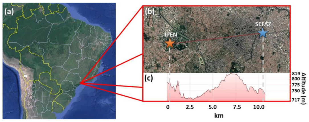
2.1. São Paulo Megacity

São Paulo is the most populous Brazilian city, with around 12.3 million inhabitants distributed in an urban area of 1521 km² [33]. It is situated in the “Paulista” Plateau at 700 m above sea level (asl) and about 60 km from the Atlantic Ocean (Figure 1a). São Paulo has a high elevation subtropical humid (Cwb) climate, where summers (December–February) are warm and wet, while winters (June–August) are dry and mildly cold [34].

The measurement campaign was held in São Paulo city from 22 July to 29 August 2019. During this period, two elastic lidar systems, approximately 10.7 km apart (Figure 1b), were operating from 09 to 18 Local Time (LT). The urban site, located downtown in São Paulo city (23°32′ S, 46°37′ W, 739 m above sea level), was named SEFAZ. The suburban site, located west of São Paulo city (23°34′ S, 46°43′ W, 782 m above sea level), was named IPEN.

2.2. Instrumentation

2.2.1. Metropolitan São Paulo Lidar 1 (MSP1) System

The Metropolitan São Paulo Lidar 1 (MSP1) system is a coaxial ground-based multiwavelength Raman lidar located at the Nuclear and Energy Research Institute (IPEN) in the suburban region of São Paulo city (23°34′ S, 46°43′ W, 782 m asl) (Figure 1b). MSP1 operates with a pulsed Nd:YAG laser pointed towards the zenith direction, emitting radiation at 355 nm, 532 nm, and 1064 nm with a repetition frequency of 10 Hz. This system detects three Raman-shifted channels (387, 408, and 530 nm) and three elastic channels (355, 532, and 1064 nm), reaching the full overlap at 300 m above ground level [7]. During the field campaign, MSP1 was run with a temporal and spatial resolution of 1 min and 7.5 m, respectively, from 09 to 18 LT.

2.2.2. Metropolitan São Paulo Lidar (MSP) 2 System

The Metropolitan São Paulo Lidar 2 (MSP2) is a mobile biaxial ground-based multiwavelength Raman lidar system. MSP2 operates with a pulsed Nd: YAG laser, which emits radiation at 355 nm and 532 nm in the zenith direction and detects one elastic channel (532 nm) and one Raman-shifted channel (387 nm). Such a system reaches the full overlap at 180 m above ground level. During the field campaign, this system was allocated in the Department of the Treasury of the São Paulo State (SEFAZ) in the urban region of São Paulo city (23°32′ S, 46°37′ W, 739 m asl) (Figure 1b), operating continuously with a temporal and spatial resolution of 1 min and 7.5 m, respectively.

2.2.3. Suomi National Polar-Orbiting Partnership (Suomi NPP) Data

The Suomi National Polar-orbiting Partnership (Suomi NPP) is a weather satellite operated by the National Oceanic and Atmospheric Administration (NOAA). Launched in 2011, Suomi NPP is equipped with the Visible Infrared Imaging Radiometer Suite (VIIRS) and the Ozone Mapping and Profiling Suite Nadir-Mapper (OMPS-NM). The VIIRS is a whiskbroom scanner radiometer, which passively observes reflectance at visible and infrared wavelengths [35].

In this work, Aerosol Optical Depth (AOD) and Aerosol Index (AI) were obtained respectively from VIIRS data and normalized radiances using two-wavelength pairs at 340 and 378.5 nm of OMPS-NM. AI is a qualitative index that indicates the presence of aerosol layers, such as biomass-burning, desert-dust, and volcanic-ash plumes, monitoring the absorption in the above-mentioned wavelength pairs [36]. Both datasets are available at: https://earthdata.nasa.gov (accessed on 1 March 2021).

2.2.4. AERONET Sunphotometer

The AErosol RObotic NETwork (AERONET) [37] is the NASA sunphotometer global network that supplies automatic sun and sky scanning measurements. Using direct sun measurements, AERONET supplies both Aerosol Optical Depth (AOD) and the Ångström Exponent (Å), which gives the wavelength dependence of the AOD. Using multiangular and multispectral measurements of atmospheric radiance and applying a flexible inversion algorithm [38], the AERONET data can also supply several additional aerosol optical and microphysical parameters, such as size distribution, single-scattering albedo, and refractive index. The operating principle of this system is to acquire aureole and sky radiance observations using a large number of solar scattering angles through a constant aerosol profile and thus retrieve the aerosol size distribution, the phase function, and the AOD [39]. In this work, the AERONET sunphotometer data were measured in the SP-EACH station located in São Paulo city (23°48′ S, 46°49′ W, 754 m asl). These data were used to derive the aerosol size distribution and Angstrom Matrix during the BB event from 17 to 19 August 2019.

3. Methodology

3.1. PBLH Detection

The PBLH was estimated from the 532 nm backscattered signal, so the algorithm is divided into two parts: raw lidar data pre-processing [40] and Wavelet Covariance Transform (WCT) algorithm [14]. The data pre-processing begins with the subtraction of the dark current signal (DC(z)) of the raw lidar signal (P) to reduce the influence of electrical noise. Then, the background radiation signal (BG) is removed to attenuate the influence of external sources. Finally, due to the attenuation of the lidar signal with the height, the result of the previous steps is multiplied by the square of the corresponding height (z), resulting in the Range Corrected Signal (RCS₅₃₂), as indicated in Equation (1):

RCS₅₃₂(z) = (P(z) − DC(z) − BG) × z²,

(1)

After the raw signal pre-processing, the second part of the algorithm is performed, where the WCT algorithm is applied. Firstly, the covariance ($\mathrm{W}\left(\mathrm{a},\mathrm{b}\right)$) between the average RCS₅₃₂(z) obtained for one hour (${\overline{\mathrm{RCS}}}_{532}$(z)) and Haar function ($\mathrm{h}\left(\frac{\mathrm{z}-\mathrm{b}}{\mathrm{a}}\right)$), the mother-wavelet is done:

$$\mathrm{W}\left(\mathrm{a},\mathrm{b}\right)=\frac{1}{\mathrm{a}}{{\displaystyle \int }}_{{\mathrm{z}}_{\mathrm{i}}}^{{\mathrm{z}}_{\mathrm{f}}}{\overline{\mathrm{RCS}}}_{532}\left(\mathrm{z}\right)\mathrm{h}\left(\frac{\mathrm{z}-\mathrm{b}}{\mathrm{a}}\right)\mathrm{dz},$$

(2)

where z is the height above the ground, z_i and z_f are the lower and upper limit of the ${\overline{\mathrm{RCS}}}_{532}$(z), respectively, and the respective values of dilatation and transition-related to mother-wavelet are given by a and b. Considering a previous study by Moreira et al. [41], which was held in São Paulo city, the parameters a and b received the values 200 and 40 m, respectively. Then, the height z where the maximum $\mathrm{W}\left(\mathrm{a},\mathrm{b}\right)$ occurs is classified as PBLH:

$$\mathrm{PBLH}=\mathrm{Max}\left(\mathrm{W}\left(\mathrm{a},\mathrm{b}\right)\right),$$

(3)

3.2. PBLH Levelness

The Levelness number (L) was defined by Stull [42] as:

$$\mathrm{L}=\Delta {\mathrm{z}}_{\mathrm{i}}/\Delta {\mathrm{z}}_{\mathrm{T}},$$

(4)

where $\Delta {\mathrm{z}}_{\mathrm{i}}$ and $\Delta {\mathrm{z}}_{\mathrm{T}}$ are PBLH and topography differences, respectively. The ratio L provides information about how the PBLH varies horizontally with respect to the topographic variations. If L < 0, the PBLH varies in an opposite way to the topography, that is, the higher terrains have lower PBLH values and vice-versa. L = 0 indicates that PBLH remains level concerning the surface. When L = 1, the PBLH follows topography, in other words, higher terrains have higher PBLH values and vice-versa. Finally, L > 1 indicates that the amplitude (absolute value) of PBLH differences is larger than topographic ones, so higher (lower) terrain has much higher (lower) PBLH.

In the case of São Paulo city $\Delta {\mathrm{z}}_{\mathrm{i}}={\mathrm{PBLH}}_{\mathrm{SEFAZ}}-{\mathrm{PBLH}}_{\mathrm{IPEN}}$ and $\Delta {\mathrm{z}}_{\mathrm{T}}$ = −57 m is the difference between the altitude of SEFAZ and IPEN lidar sites. To take advantage of the high spatial resolution of lidar systems (~7.5 m) used in São Paulo, cases L = 1 and L = 0 are replaced by L~1 and L~0, respectively. L~1 represents cases where L is closer to 1 than to 0, and PBLH tends to follow topography. As the difference between SEFAZ and IPEN altitudes $\Delta {\mathrm{z}}_{\mathrm{T}}$ = −57 m, L~1 occurs when 57 m $\ge \left|\Delta {\mathrm{z}}_{\mathrm{i}}\right|\ge$ 29 m (

Table 1. Behavior classes of PBLH with respect to topography based on Levelness number (L) for São Paulo city. Classes of L are estimated in terms of PBLH ($\Delta {\mathrm{z}}_{\mathrm{i}}$) and topography ($\Delta {\mathrm{z}}_{\mathrm{T}}$) differences for SEFAZ and IPEN lidar sites. The background colors for each line represent the colors that will be used to illustrate the behavior of L in the next figures.

L	Δzi = PBLHSEFAZ − PBLHIPEN	Behavior of PBLH with Respect to Topography
L < 0	Δzi > 29 m	PBLH varies opposite to topography
L~0	|Δzi| < 29 m	PBLH tends to level
L~1	−57 m ≥ Δzi ≥ −29 m	PBLH tends to follow the topography
L > 1	Δzi < −57 m	PBLH differences are larger than topographic ones

). On the other hand, L~0 indicates the cases where L is closer to 0 than to 1, and the PBLH tends to level when $\left|\Delta {\mathrm{z}}_{\mathrm{i}}\right|$ < 29 m. Table 1 summarizes how L and $\Delta {\mathrm{z}}_{\mathrm{i}}$ are related in the case of São Paulo city.

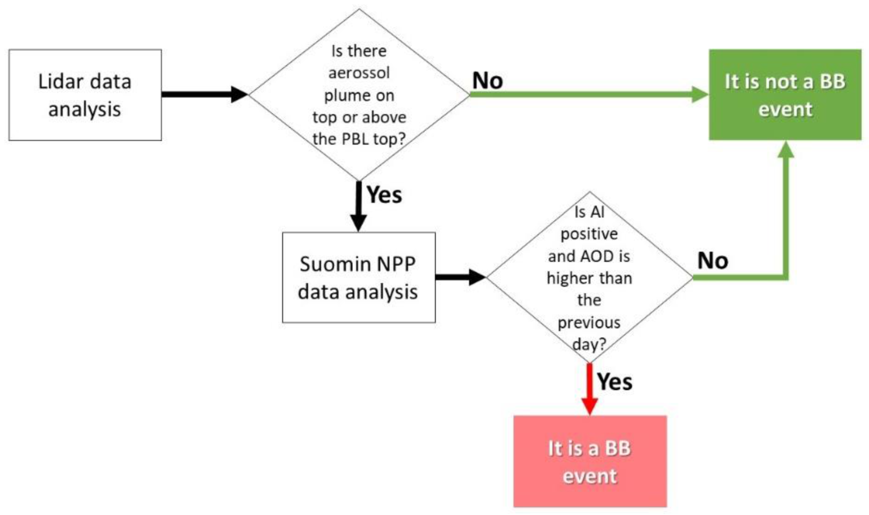
3.3. Detection Algorithm of BB Events

Earlier studies show that in São Paulo city, the BB events are, in general, associated with the presence of high-concentration aerosol layers in the first 5 km of the atmosphere [10,25]. They occur between May and October when the number of forest fires in the center-west Brazil and Amazon regions and the burning of organic matter produced in the sugarcane crops in the countryside of São Paulo State [10,25] increases.

The intense aerosol loading combined with high solar radiation absorption capacity let these BB events be identified by the simultaneous increase in the daily values of Aerosol Optical Depth (AOD) and Aerosol Index (AI) [43,44]. Therefore, in this work, a new detection algorithm for BB events was developed and applied to São Paulo city. As displayed schematically in Figure 2, this algorithm combines key properties of lidar and satellite data. First, lidar data are used to find the aerosol layers. In the case of a positive outcome, daily values of AOD and AI are estimated for the lidar site and compared with corresponding daily values in the previous day.

As there is no evidence that São Paulo city is affected by dust outbreaks, identifying the BB event is necessary only to verify whether daily values of AI remain positive during two consecutive days. To track the origin of the BB event is necessary to verify whether AOD daily values are increasing during these two consecutive days when AI values were positive. If both conditions are satisfied, it is plausible to infer that the aerosol layer detected in São Paulo was produced by a BB event and VIIRS data can be used to identify its origin.

4. Results

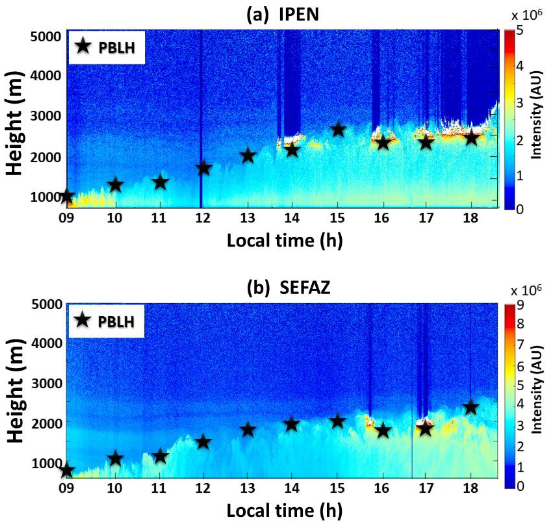
4.1. PBLH Horizontal Variation

In this section, the diurnal evolution of differences between PBLH retrieved at IPEN (PBLH_IPEN) and SEFAZ (PBLH_SEFAZ) from lidar measurements is analyzed. Firstly, two case studies illustrate how the absence (23 July 2019) and presence (8 August 2019) of low clouds affect the relationship between PBLH and topographic difference during the day. Then, a statistical analysis of the PBLH behavior is discussed, considering observations carried out for 12 days selected is also presented. It is important to emphasize that sea-breeze circulation is observed with frequency in São Paulo city [31]; however, sea breeze circulation was not observed on 23 July and 8 August 2019.

4.1.1. Case 1: Absence of Low Clouds

The diurnal evolution of PBLH is shown (by black stars) in the RCS-Intensity curtain plots of 23 July 2019 at IPEN (Figure 3a) and SEFAZ (Figure 3b). Due to technical differences in the lidar systems and possible spatial variation in the aerosol concentrations, the RCS intensities observed in both sites are not the same. However, the vertical structure of the aerosol layers is quite similar. This day is characterized by the absence of low clouds and the aerosol layer adjacent to the surface is well mixed, consequently a well-defined PBL in both sites. There is a thin aerosol layer (purple dashed boxes in Figure 3a,b) above the PBL, between 2000 and 3000 m, in both sites. As demonstrated, the Section 4.2 aerosol layers aloft the PBL may result from BB events advected into São Paulo city.

At IPEN (Figure 3a), the PBLH remains practically constant from 09 to 11 LT, and it has a fast-growth stage from 12 to 14 LT reaching 1400.0 ± 7.5 m. Then, from 15 to 18 LT, PBLH remains practically constant and equal to 1452.0 ± 7.5 m.

At SEFAZ (Figure 3b), the PBLH displayed a longer fast-growth stage from 09 to 13 LT, reaching 1390.0 ± 7.5 m. At 15 LT, the PBLH reaches its maximum value of 1460.0 ± 7.5 m and maintains constant until 18 LT.

Figure 4 display the diurnal evolution of PBLH_SEFAZ-PBLH_IPEN (Δz_i) and PBLH Levelness (L) on 23 July 2019. The higher differences occur during the growth stage because PBLH_SEFAZ and PBLH_IPEN displayed different growth rates (156.7 and 153.0 m·h⁻¹, respectively), which is probably associated with the land use of each region (IPEN–suburban, SEFAZ–urban). Comparatively, on most mornings, PBLH_SEFAZ is higher and has larger growth rate values than PBLH_IPEN. Such behavior is expected because the sensible heat flux in the urban region (SEFAZ) is expected to be higher than in the suburban region (IPEN). The maximum difference (Δz_i = 300.0 ± 10.6 m) was observed at 12 LT when PBLH_SEFAZ reached the mature stage and PBLH_IPEN just started the fast-growth stage. After the fast growth stage, at 14 LT, PBLH_IPEN and PBLH_SEFAZ displayed similar behavior, reaching a remarkably similar maximum value and remaining almost constant until the end of the day. During this period, an intense reduction in the difference between the PBLH values occurs (Δz_i = 8.0 ± 10.6 m).

Regarding L, during the first two hours (09 to 10 LT), while the fast PBL-growth stage has not started, the PBLH tends to level (L~0). During the fast-growth stage (11 to 13 LT), PBLH varies horizontally opposite to topography because the growth rate at SEFAZ is higher than at IPEN (L < 0). However, at 14 LT, when both PBL are almost fully developed, the PBLH tends to level again (L~0). This result agrees with Stull [42], which indicates that the PBLH tends to level when it is fully developed.

4.1.2. Case 2: Presence of Low Clouds

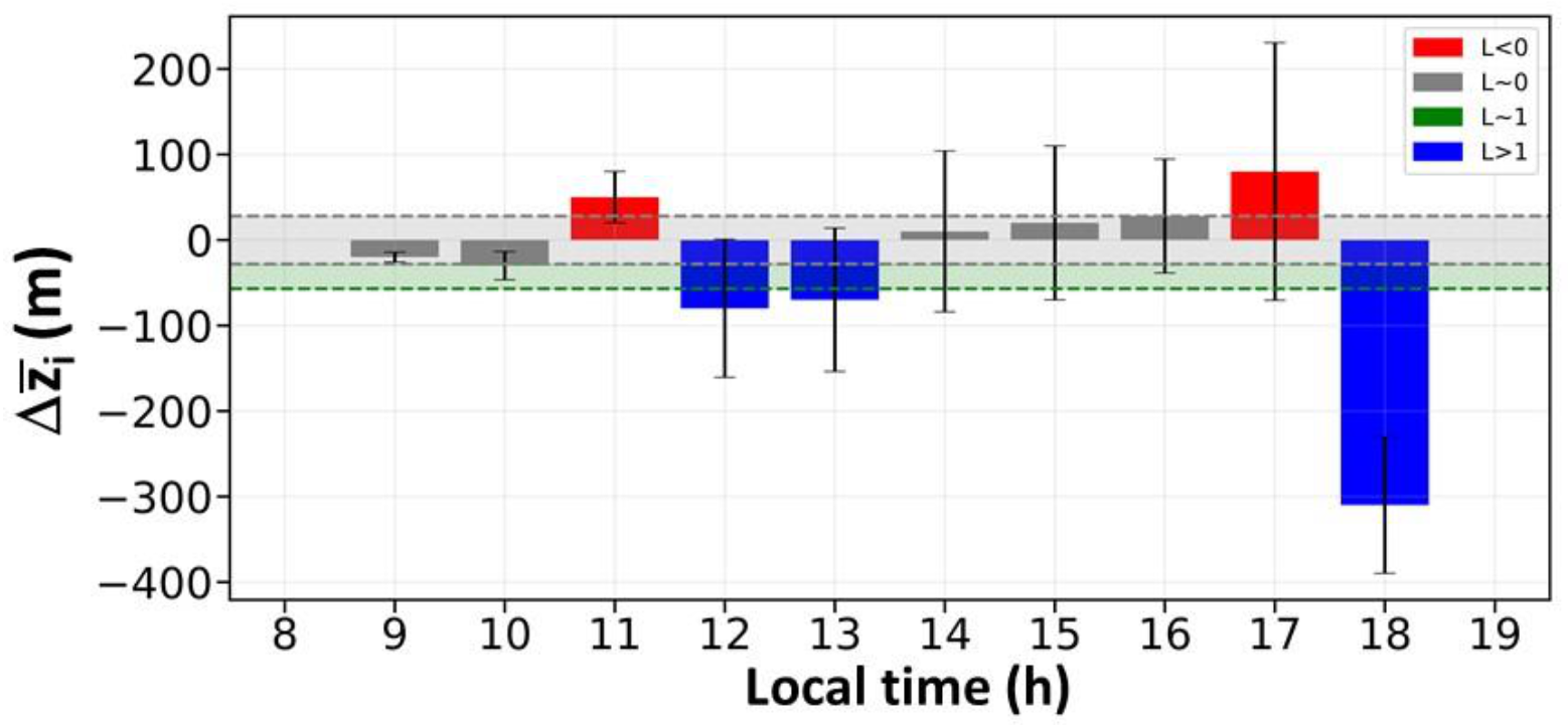
The diurnal evolution of PBLH is shown (by black stars) in the RCS-Intensity curtain plots on 8 August 2019 at IPEN (Figure 5a) and SEFAZ (Figure 5b). This day is characterized by the presence of scattered low clouds at both sites.

At IPEN, PBLH_IPEN displays a fast-growth stage from 09 to 15 LT, reaching its maximum value of 2600 ± 7.5 m. The presence of scattered low clouds affected the performance of the WTC method, which tends to retrieve PBLH as the base of the cloud [15]. During the afternoon, the presence of clouds became more frequent in both sites, and PBLH was retrieved below the actual PBLH, indicating that the cloud base was below the actual PBLH in the IPEN site. Between 16 and 18 LT, PBLH was retrieved below the actual PBLH, indicating that the cloud base was below the actual PBLH.

At SEFAZ, PBLH_SEFAZ displays a fast-growth stage from 09 to 14 LT. Between 15:30 and 17 LT, the presence of scattered low clouds affected the performance of the PBLH-detection algorithm so that hourly values of PBLH retrieved from the WCT method were misplaced below the actual PBLH. At 18 LT, PBLH_SEFAZ reaches its maximum daily value of 2400 ± 7.5 m.

Like the previous case, PBLH_IPEN and PBLH_SEFAZ display different growth rates (266.7 and 166.7 m·h⁻¹, respectively). However, in this case, the PBLH_IPEN grows faster than PBLH_SEFAZ from 9 to 14 LT (Figure 5), indicating that other causes rather than land use are affecting the diurnal evolution of PBLH in both sites.

Regarding L, it remains >1 during the fast-growth stage (09–13 LT) and most of the mature stage (15–17 LT), indicating that the amplitude of the absolute values of PBLH differences are systematically larger than topographic ones. The higher Δz_i value (−500 ± 10.6 m) is observed during the mature stage period. Comparatively to the fast-growth stage, the frequency of low clouds is higher during the mature stage in both sites (Figure 5). At 14 LT, no clouds were identified by both lidars sites (Figure 5), the growth rate of PBLH_IPEN and PBLH_SEFAZ are equally attenuated, and the PBLH difference decreases significantly (Δz_i = −48 ± 10.6 m). As indicated by L~1 at 14 LT (Figure 6), the PBLH tends to follow the topography. At 18 LT, the presence of low clouds was observed only in the IPEN region. As a result, PBLH differences become smaller than Δz_i (56 ± 10.6 m), and, as indicated by L < 0, PBLH difference varies in the opposite way to the topography one.

Based on the above analysis, it seems plausible to infer that the presence of clouds has affected the diurnal evolution of PBLH in both sites by keeping the PBLH differences between SEFAZ and IPEN negative, which contradicts the expected land-use effect ng and by increasing it in absolute terms during the afternoon.

The presence of low clouds intensifies the vertical mixing, mainly inside the cloud, reducing or even eliminating the presence of aerosol layers aloft at the PBL site. Several aerosol layers present in the first 3 km of the atmosphere at the IPEN (Figure 5a) were diluted after 13 LT and incorporated the PBL totally at 15 LT. While at SEFAZ (Figure 5b), higher aerosol layers remain above the PBL during the 17 LT. As will be shown in Section 4.2 below, these aerosol layers are composed of black carbons produced by BB events advected to São Paulo city during winter. During the daytime, they absorb incoming solar radiation, heating the atmosphere locally between 2 and 3 km. This localizing heat generates elevated inversion layers that, in turn, inhibit the vertical evolution of the PBL. This mechanism seems to be acting on 23 July 2019, when no low clouds were detected, restricting the vertical evolution of PBL to 1450 m in IPEN (Figure 3a) and SEFAZ (Figure 3b). On 8 August 2019, the presence of low clouds disrupted the process of stabilization induced by the aerosol layers from BB events, allowing a much deeper vertical evolution of the PBL, but as indicated in the Figure 5a,b, clouds were more frequent over IPEN than SEFAZ, so that the PBL differences remain negative during almost the entire daytime and becomes more intense during the afternoon when the presence of low clouds are more intense at IPEN site.

4.1.3. All Campaign

The diurnal evolution of statistical properties of PBLH_IPEN and PBLH_SEFAZ, as well as their respective mean values (${\overline{\mathrm{PBLH}}}_{\mathrm{IPEN}}$ and ${\overline{\mathrm{PBLH}}}_{\mathrm{SEFAZ}}$), retrieved from lidar performed in SEFAZ and IPEN during the 12 days of the field campaign, are presented in Figure 7.

From 09 to 10 LT, PBLH_IPEN and PBLH_SEFAZ have low variability and similar evolutions. At 11 LT, PBLH_SEFAZ has greater variability and mean value. Between 12 and 13 LT, PBLH_SEFAZ has the greatest variability, but ${\overline{\mathrm{PBLH}}}_{\mathrm{IPEN}}$ is higher than ${\overline{\mathrm{PBLH}}}_{\mathrm{SEFAZ}}$. Between 14 and 16 LT, both distributions and mean values of PBLH_IPEN and PBLH_SEFAZ have very similar behavior so considering the statistical error, ${\overline{\mathrm{PBLH}}}_{\mathrm{IPEN}}$ and ${\overline{\mathrm{PBLH}}}_{\mathrm{SEFAZ}}$ are equal. The maximum values of ${\overline{\mathrm{PBLH}}}_{\mathrm{IPEN}}$ (1600.0 ± 38.7 m) and ${\overline{\mathrm{PBLH}}}_{\mathrm{SEFAZ}}$ (1630.0 ± 54.2 m) are observed at 16 LT. At 17 LT, PBLH_IPEN has high variability and an average value less than PBLH_SEFAZ. However, considering the statistical error, ${\overline{\mathrm{PBLH}}}_{\mathrm{IPEN}}$ (1520.0 ± 129.0 m) and ${\overline{\mathrm{PBLH}}}_{\mathrm{SEFAZ}}$ (1600.0 ± 77.4 m).

At 18 LT, PBLH_SEFAZ has greater variability than PBLH_IPEN and a predominance of smaller values. Such an effect is caused by the sea breeze, which systematically penetrates more than 50% of all days of the year in São Paulo city [31]. The sea breeze brings colder and more moist air from the coast, changing the vertical aerosol distribution and causing a high aerosol concentration in the lower part of the PBL. Then, methods based on the vertical aerosol gradient (e.g., WCT) tend to underestimate the PBLH in this situation [7]. Analyzing high-resolution data from numerical simulation with WRF Model, Ribeiro et al. [32] also show that the passage of sea breeze during the afternoon induces a significant drop in the PBLH in São Paulo city.

Figure 8 presents the diurnal evolution of the levelness parameter and the difference between ${\overline{\mathrm{PBLH}}}_{\mathrm{SEFAZ}}$ and ${\overline{\mathrm{PBLH}}}_{\mathrm{IPEN}}$ ($\Delta \overline{{\mathrm{z}}_{\mathrm{i}}}$). From 09 to 10 LT, the average Δz_i remains below |28| m so that during this period, the PBLH tends to level (L~0). At 11 LT, PBLH_SEFAZ display a large growth rate, Δz_i intensifies, reaching 55 ± 30.7 m and the average horizontal variation of PBLH is opposite to the topography (L < 1). Between 12 and 13 LT, the average PBLH displays the most intense growth rate in both sites and Δz_i becomes greater, so that the PBLH varies horizontally, amplifying topographic differences (L > 1). From 14 to 16 LT, the period in which ${\overline{\mathrm{PBLH}}}_{\mathrm{SEFAZ}}$ and ${\overline{\mathrm{PBLH}}}_{\mathrm{IPEN}}$ have little variation, Δz_i is again smaller than 28 m, and PBLH tends to levelling (L~0). At 17 LT, due to the reduction in the mean value of PBLH_IPEN, PBLH varies horizontally as opposed to topography (L < 0). Then, at 18 LT, the PBLH_SEFAZ reduces sharply so that the PBLH varies, intensifying the topographical differences (L > 1). Such a phenomenon occurs due to the presence of the sea breeze, which arrives first at the SEFAZ, later spreading to the IPEN region. However, due to slow sea breeze displacement in urban areas [32,42], at 18 LT, only the SEFAZ region was reached by it. So, PBLH_SEFAZ has a significant drop (Figure 7), becoming lower than PBLH_IPEN.

It is important to emphasize that the effects of thermal stabilization associated with the presence of aerosol layers associated with BB events on average seem to be canceled out by the effect of low clouds so that PBLH differences between SEFAZ and IPEN are very small.

4.2. Biomass Burning Detection

Figure 9 shows the RCS-Intensity curtain plots measured by the lidar at the SEFAZ on 19 August 2019. From 06 to 13 LT, an intense aerosol plume (dashed violet box) extends from 1000 m to the PBLH_SEFAZ. In the presence of intense aerosol plumes, such as the BB event on 19 August, the lidar methods based on the aerosol gradient tend to retrieve PBLH at the top of the aerosol layer. Therefore, the behavior of PBLH_SEFAZ between 09 and 12 LT does not necessarily represent the real top of the PBL [2,13]. Indeed, on average, the PBLH displays a fast-growth stage during this period (Figure 7b). From 22 LT until the end of the measurements at 24 LT, a shallow layer with high aerosol concentration appeared near the surface, causing an intense backscattering and impeding laser signal to reach above this shallow layer.

Figure 10 presents the spatial distribution of AI in Brazil, Paraguay, Bolivia, northern Argentina, and Uruguay from 17 to 19 August 2019. On 17 August, an aerosol plume, with AI values ranging between 2 and 5, was observed near the Bolivia–Brazil frontier. With the predominance of AI values higher than 3, the aerosol plume occupied a large horizontal extension on 18 August, spreading from the Brazil–Bolivia frontier to the Midwest region of Brazil. On 19 August, the aerosol plume was displaying AI values around 5. Located entirely in Brazil, this aerosol plume covered the States of São Paulo, Mato Grosso do Sul, Minas Gerais, and Rio de Janeiro.

Figure 11 presents the variation of AOD in Brazil, Paraguay, Bolivia, and the northern region of Argentina and Uruguay, from 17 to 19 August 2019. On 17 August, while low values of AOD could be observed over southeastern Brazil, where São Paulo city is located, high AOD values (AOD > 0.8) were detected in the Brazil–Bolivia frontier. On 18 August, the area with high AOD values (>0.8) moved to the region between Brazil–Bolivia frontier and the Brazilian Midwest, coinciding with the aerosol plume shown in Figure 10. On the other hand, the AOD value for the visible region (without clouds) in the São Paulo city area remains below 0.2. On 19 August, despite the presence of clouds, it is possible to observe that AOD values are approximately 1 from the Brazilian Midwest to the São Paulo city area. Therefore, AOD values increased significantly in São Paulo city on 19 August in comparison to the previous two days.

Inversion data from SP-EACH AERONET sunphotometer station were employed to derive the log-normal size distribution of aerosol from 17 to 19 August 2019. As shown in Figure 12, the log-normal distribution on 17 August changes during the day. However, fine mode aerosols are dominant during the whole period and there is strong evidence that most aerosols come from the BB event produced by the wildfires on the Brazil–Bolivia frontier.

According to Cazorla et al., 2012 [45], the chemical composition of aerosol can be identified from the Ångström Matrix. It consists of a dispersion diagram of Scattering Ångström Exponent (SAE) by Absorption Ångström Exponent (AAE). The sub-sections of this diagram define aerosol composition by grouping absorbing aerosol types [46,47]. During the aerosol transport event that occurred between 17 and 19 August over MRSP, the Ångström Matrix in Figure 13 shows the presence of small particles with low absorption, with some cases of black carbon aerosol composition.

Therefore, based on the methodology presented in Section 3.3, it is possible to conclude that the intense aerosol layer observed on 19 August 2019 represents a BB event. Such a result is in accordance with Pereira et al. (2021) [48], who from a combination of back trajectory analyses (from Hybrid Single-Particle Lagrangian Integrated Trajectory [49]) and images from satellite (GOES-16 Advanced Baseline Instrument and Moderate Resolution Imaging Spectroradiometer) observed air masses transporting plumes of biomass burning aerosols from Bolivia and the Amazon Basin to São Paulo state. Such a BB event was widely publicized in the press due to its unprecedented effects, such as “black rain” [48], which could be detected in several regions of the São Paulo state.

In the 12 days of measurements, strong aerosol plumes above or on the PBL top were found in 3 of them (23 July, 10 and 19 August 2019), but only on 10 August variations in AOD and AI could be associated with the presence of material from biomass burning.

5. Conclusions

Elastic lidar systems have been widely applied in studies related to PBL structure. The high spatial and temporal resolutions of this type of remote sensing system allow it to be used in several environmental applications. In this work, data from two elastic LIDAR systems, which operated simultaneously at approximately 10.7 km of distance, were used to analyze the homogeneity of the PBLH in the city of São Paulo. In addition, a new procedure based on elastic lidar and satellites data were used to identify the impact of BB events in the aerosol layer detected above the PBL.

Except for the cases with the presence of sea breezes, in general, higher differences in the PBLH horizontal homogeneity (around 100 m) are observed during its growth period. Before the PBL growth stage and when the PBLH is fully developed, it was observed that PBLH tends to levelling (L~0). Sea breeze moves slowly in urban areas, so its presence makes the PBLH vary horizontally, amplifying topographical differences (L > 1). Furthermore, a stabilization of the atmosphere caused by the presence of aerosol layers associated with BB events was observed. However, such a result needs a more intensive investigation using radiosonde data to identify the presence of thermal inversion induced by these aerosol layers.

In addition, the synergy between the elastic lidar and satellites data enabled the detection of a BB event, as well as identifying its origin. Such a result demonstrates that the proposed methodology is an efficient and easy-applicable tool to detect BB events in São Paulo city. However, it is necessary to extend the application to a larger set of cases, using AE as a benchmark.

Therefore, these results reinforce the great importance and applicability of elastic lidar systems in PBL studies. So that the combination of a set of lidar systems or a synergy use of lidars and other remote sensing systems can provide a better understanding of certain phenomena.

References

1. Lange, D.; Tiana-alsina, J.; Saeed, U.; Tomás, S.; Rocadenbosch, F. Using a Kalman Filter and Backscatter Lidar Returns. IEEE Trans. Geosci. Remote. Sens. 2014, 52, 4717–4728. [Google Scholar] [CrossRef]
2. Bravo-Aranda, J.A.; de Arruda Moreira, G.; Navas-Guzmán, F.; Granados-Muñoz, M.J.; Guerrero-Rascado, J.L.; Pozo-Vázquez, D.; Arbizu-Barrena, C.; Olmo-Reyes, F.J.; Mallet, M.; Alados-Arboledas, L. A new methodology for PBL height estimations based on lidar depolarization measurements: Analysis and comparison against MWR and WRF model-based results. Atmos. Chem. Phys. 2017, 17, 6839–6851. [Google Scholar] [CrossRef] [Green Version]
3. Moreira, G.A.; Guerrero-Rascado, J.L.; Benavent-Oltra, J.A.; Ortiz-Amezcua, P.; Román, R.; Bedoya-Velásquez, A.E.; Bravo-Aranda, J.A.; Olmo Reyes, F.J.; Landulfo, E.; Alados-Arboledas, L. Analyzing the turbulent planetary boundary layer by remote sensing systems: The Doppler wind lidar, aerosol elastic lidar and microwave radiometer. Atmos. Chem. Phys. 2019, 19, 1263–1280. [Google Scholar] [CrossRef] [Green Version]
4. Liu, B.; Ma, Y.; Gong, W.; Zhang, M.; Yang, J. Improved two-wavelength Lidar algorithm for retrieving atmospheric boundary layer height. J. Quant. Spectrosc. Radiat. Transf. 2019, 224, 55–61. [Google Scholar] [CrossRef]
5. Lopes, F.J.S.; Moreira, G.A.; Rodrigues, P.F.; Guerrero-Rascado, J.L.; Andrade, M.F.; Landulfo, E. Lidar measurements of tropospheric aerosol and water vapor profiles during the winter season campaigns over the metropolitan area of Sao Paulo, Brazil. In Proceedings of the Lidar Technologies, Techniques, and Measurements for Atmospheric Remote Sensing X. International Society for Optics and Photonics, San Diego, CA, USA, 20 October 2014; p. 92460H. [Google Scholar] [CrossRef]
6. Ma, X.; Wang, C.; Han, G.; Ma, Y.; Li, S.; Gong, W.; Chen, J. Regional Atmospheric Aerosol Pollution Detection Based on LiDAR Remote Sensing. Rem. Sens. 2019, 11, 2339. [Google Scholar] [CrossRef] [Green Version]
7. Moreira, G.A.; da Silva Lopes, F.J.; Guerrero-Rascado, J.L.; da Silva, J.J.; Arleques Gomes, A.; Landulfo, E.; Alados-Arboledas, L. Analyzing the atmospheric boundary layer using high-order moments obtained from multiwavelength lidar data: Impact of wavelength choice. Atmos. Meas. Tech. 2019, 12, 4261–4276. [Google Scholar] [CrossRef] [Green Version]
8. Hu, Y.; Lu, X.; Zhai, P.; Hostetler, C.A.; Hair, J.W.; Cairns, B.; Sun, W.; Stamnes, S.; Omar, A.; Baize, R.; et al. Liquid phase cloud microphysical property estimates from CALIPSO measurements. Front. Remote. Sens. 2021, 2, 724615. [Google Scholar] [CrossRef]
9. Moreira, G.A.; Guerrero-Rascado, J.L.; Bravo-Aranda, J.A.; Foyo-Moreno, I.; Cazorla, A.; Alados, I.; Lyamani, H.; Landulfo, E.; Alados-Arboledas, L. Study of the planetary boundary layer height in an urban environment using a combination of microwave radiometer and ceilometer. Atmos. Res. 2020, 240, 104932. [Google Scholar] [CrossRef]
10. Mariano, G.L.; Lopes, F.J.S.; Jorge, M.P.O.M.; Landulfo, E. Assessment of biomass burnings activity with synergy of sunphotometric and LIDAR measurements in São Paulo, Brazil. Atmos. Res. 2010, 98, 486–499. [Google Scholar] [CrossRef]
11. Lopez, D.H.; Rabbani, M.R.; Crosbie, E.; Raman, A.; Arellano, A.F.; Sorooshian, A. Frequency and Character of Extreme Aerosol Events in the Southwestern United States: A Case Study Analysis in Arizona. Atmosphere 2016, 7, 1. [Google Scholar] [CrossRef] [Green Version]
12. Chan, K.L. Biomass burning source and their contributions to the local air quality in Hong Kong. Scien. Tot. Environ. 2017, 596, 212–221. [Google Scholar] [CrossRef]
13. Kovalev, A.V.; Eichinger, E.W. Elastic Lidar: Theory, Practice and Analysis Methods; Willey Interscience: Hoboken, NJ, USA, 2004. [Google Scholar]
14. Baars, H.; Ansmann, A.; Engelmann, R.; Althausen, D. Continuous monitoring of the boundary-layer top with lidar. Atmos. Chem. Phys. 2008, 8, 10749–10790. [Google Scholar] [CrossRef] [Green Version]
15. Emeis, S. Surface-Based Remote Sensing of the Atmospheric Boundary Layer; Springer: Berlin, Germany, 2011. [Google Scholar]
16. Ribeiro, F.N.D.; Soares, J.; Oliveira, A.P. The Co-Influence of the sea breeze and the coastal upwelling at Cabo Frio: A numerical investigation using coupled models. Braz. J. Oceanogr. 2011, 59, 131–144. [Google Scholar] [CrossRef] [Green Version]
17. Finnigan, J.; Ayotte, K.; Harman, I.; Katul, G.; Oldroyd, H.; Patton, E.; Poggi, D.; Ross, A.; Taylor, P. Boundary-Layer Flow over Complex Topography. Bound.-Layer Meteorol. 2020, 177, 247–313. [Google Scholar] [CrossRef]
18. Barlow, J.F.; Halios, C.H.; Lane, S.E.; Wood, C.R. Observations of urban boundary layer structure during a strong urban heat island event. Env. Fluid Mech. 2015, 15, 373–398. [Google Scholar] [CrossRef] [Green Version]
19. De Wekker, S.F.J.; Kossmann, M. Convective Boundary Layer Heights over Mountainous Terrain—A Review of Concepts. Front. Earth Sci. 2015, 3, 77. [Google Scholar] [CrossRef] [Green Version]
20. Fernández, A.J.; Sicard, M.; Costa, M.J.; Guerrero-Rascado, J.L.; Gómez-Amo, J.L.; Molero, F.; Barragán, R.; Basart, S.; Bortoli, D.; Bedoya-Velásquez, A.E.; et al. Extreme, wintertime Saharan dust intrusion in the Iberian Peninsula: Lidar monitoring and evaluation of dust forecast models during the February 2017 event. Atmos. Res. 2019, 228, 223–241. [Google Scholar] [CrossRef]
21. Gonzalez, M.E.; Garfield, J.G.; Corral, A.F.; Edwards, E.-L.; Zeider, K.; Sorooshian, A. Extreme Aerosol Events at Mesa Verde, Colorado: Implications for Air Quality Management. Atmosphere 2021, 12, 1140. [Google Scholar] [CrossRef]
22. Marques, J.F.; Alves, M.B.; Silveira, C.F.; Silva, A.A.; Silva, T.A.; Santos, V.J.; Calijuri, M.L. Fires dynamics in the Pantanal: Impacts of anthropogenic activities and climate change. J. Environ. Manag. 2021, 299, 113586. [Google Scholar] [CrossRef]
23. da Silva, S.S.; Oliveira, I.; Morello, T.F.; Anderson, L.O.; Karlokoski, A.; Brando, P.M.; de Melo, A.W.F.; da Costa, J.G.; de Souza, F.S.C.; da Silva, I.S.; et al. Burning in southwestern Brazilian Amazonia, 2016–2019. J. Environ. Manag. 2021, 286, 112189. [Google Scholar] [CrossRef]
24. Landulfo, E.; Lopes, F.J.S.; Mariano, G.L.; Torres, A.S.; Jesus, W.C.; Nakaema, W.M.; Jorge, M.P.P.M.; Mariani, R. Study of the Properties of Aerosols and the Air Quality Index Using a Backscatter Lidar System and Aeronet Sunphotometer in the City of São Paulo, Brazil. J. Air Waste Manag. Assoc. 2010, 60, 386–392. [Google Scholar] [CrossRef] [PubMed] [Green Version]
25. Landulfo, E.; Lopes, F.; Landulfo, E.; Mariano, E.; Martins, M.P. Impacts of Biomass burning in the atmosphere of the southeastern region of Brazil using remote sensing systems. In Atmospheric Aerosol—Regional Characteristics—Chemistry and Physics; IntechOpen: London, UK, 2003. [Google Scholar]
26. Oliveira, P.L.; de Figueiredo, B.R.; Cardoso, A.A. Atmospheric pollutants in São Paulo state, Brazil and effects on human health—A review. Geochim. Bras. 2011, 17–24. [Google Scholar]
27. Squizzato, R.; Nogueira, T.; Martins, L.D.; Astolfo, R.; Machado, C.B.; Andrade, M.F.; Freitas, E.D. Beyond megacities: Tracking air pollution from urban areas and biomass burning in Brazil. npj Clim. Atmos. Sci. 2021, 4, 17. [Google Scholar] [CrossRef]
28. Mapbiomas Brasil. Project. Available online: https://mapbiomas.org/en/project (accessed on 12 December 2021).
29. Secretaria Municipal do Verde e do Meio Ambiente. Available online: https://www.prefeitura.sp.gov.br/cidade/secretarias/meio_ambiente/ (accessed on 12 December 2021).
30. Umezaki, A.S.; Ribeiro, F.N.D.; Oliveira, A.P.; Soares, J.; Miranda, R.M. Numerical characterization of spatial and temporal evolution of summer urban heat island intensity in São Paulo, Brazil. Urban Clim. 2020, 32, 100615. [Google Scholar] [CrossRef]
31. Oliveira, A.P.; Bornstein, R.; Soares, J. Annual and diurnal wind patterns in the city of Sao Paulo. Water Air Soil Pollut. 2003, 3, 3–15. [Google Scholar] [CrossRef]
32. Ribeiro, F.N.D.; Oliveira, A.P.; Soares, J.; Miranda, R.M.; Barlage, M.; Chen, F. Effect of sea breeze propagation on the urban boundary layer of the metropolitan region of Sao Paulo, Brazil. Atmos. Res. 2018, 214, 174–188. [Google Scholar] [CrossRef]
33. Instituto Brasileiro de Geografia e Estatística. Available online: http://ibge.gov.br (accessed on 1 December 2021).
34. Oliveira, A.P.; Marques Filho, E.P.; Ferreira, M.J.; Codato, G.; Ribeiro, F.N.D.; Landulfo, E.; Moreira, G.A.; Pereira, M.M.R.; Mlakar, P.; Boznar, M.Z.; et al. Assessing urban effects on the climate of metropolitan regions of Brazil—Preliminary results of the MCITY BRAZIL project. Explor. Environ. Sci. Res. 2020, 1, 38–77. [Google Scholar] [CrossRef]
35. Joint Polar Satellite System: Mission and Instruments. Available online: https://www.jpss.noaa.gov/mission_and_instruments.html (accessed on 30 October 2021).
36. Torres, O.; Bhartia, P.K.; Herman, J.R.; Ahmad, Z.; Gleason, J. Derivation of aerosol properties from satellite measurements of backscattered ultraviolet radiation: Theoretical basis. J. Geophys. Res. 1998, 103, 17,099–17,110. [Google Scholar] [CrossRef]
37. Holben, B.N.; Eck, T.F.; Slutsker, I.; Tanré, D.; Buis, J.P.; Setzer, A.; Vermote, E.; Reagan, J.A.; Kaufman, Y.J.; Nakajima, T.; et al. AERONET—A Federated Instrument Network and Data Archive for Aerosol Characterization. Remote Sens. Environ. 1998, 66, 1–16. [Google Scholar] [CrossRef]
38. Dubovik, O.; Smirnov, A.; Holben, B.N.; King, M.D.; Kaufman, Y.J.; Eck, T.F.; Slutsker, I. Accuracy assessments of aerosol optical properties retrieved from Aerosol Robotic Network (AERONET) Sun and sky radiance measurements. J. Geophys. Res. 2000, 105, 9791–9806. [Google Scholar] [CrossRef] [Green Version]
39. Dubovik, O.; King, M.D. A flexible inversion algorithm for retrieval of aerosol optical properties from Sun and sky radiance measurements. J. Geophys. Res. 2000, 105, 20673–20696. [Google Scholar] [CrossRef] [Green Version]
40. D’Amico, G.; Amodeo, A.; Mattis, I.; Freudenthaler, V.; Pappalardo, G. EARLINET Single Calculus Chain—Technical—Part 1: Pre-processing of raw lidar data. Atmos. Meas. Tech. 2016, 9, 491–507. [Google Scholar] [CrossRef] [Green Version]
41. Moreira, G.A.; Lopes, F.J.S.; Guerrero-Rascado, J.L.; Granados-Muñoz, M.J.; Bourayou, R.; Landulfo, E. Comparison between two algorithms based on different wavelets to obtain the Planetary Boundary Layer height. In Proceedings of the Lidar Technologies, Techniques, and Measurements for Atmospheric Remote Sensing X. International Society for Optics and Photonics, Amsterdam, The Netherlands, 20 October 2014; 2014; p. 92460D. [Google Scholar] [CrossRef]
42. Stull, R.B. A theory for mixed-layer-top levelness over irregular topography. In Proceedings of the 10th AMS Symposium on Turbulence and Diffusion (Portland), Portland, OR, USA, 29 September–2 October 1992. [Google Scholar]
43. Shi, S.; Cheng, T.; Gu, X.; Guo, H.; Wu, Y.; Wang, Y. Biomass burning aerosol characteristics for different vegetation types in different aging periods. Environ. Int. 2019, 126, 504–511. [Google Scholar] [CrossRef]
44. Liu, L.; Cheng, Y.; Wang, S.; Wei, C.; Pöhlker, M.L.; Pöhlker, C.; Artaxo, P.; Shrivastava, M.; Andreae, M.O.; Pöschl, U.; et al. Impact of biomass burning aerosols on radiation, clouds, and precipitation over the Amazon: Relative importance of aerosol–cloud and aerosol–radiation interactions. Atmos. Chem. Phys. 2020, 20, 13283–13301. [Google Scholar] [CrossRef]
45. Cazorla, A.; Bahadur, R.; Suski, K.J.; Cahill, J.F.; Chand, D.; Schmid, B.; Ramanathan, V.; Prather, K.A. Relating aerosol absorption due to soot, organic carbon, and dust to emission sources determined from in-situ chemical measurements. Atmos. Chem. Phys. 2013, 13, 9337–9350. [Google Scholar] [CrossRef] [Green Version]
46. Moosmüller, H.; Chakrabarty, R.K. Technical Note: Simple analytical relationships between Ångström coefficients of aerosol extinction, scattering, absorption, and single scattering albedo. Atmos. Chem. Phys. 2011, 11, 10677–10680. [Google Scholar] [CrossRef] [Green Version]
47. Cappa, C.D.; Kolesar, K.R.; Zhang, X.; Atkinson, D.B.; Pekour, M.S.; Zaveri, R.A.; Zelenyuk, A.; Zhang, Q. Understanding the optical properties of ambient sub- and supermicron particulate matter: Results from the CARES 2010 field study in northern California. Atmos. Chem. Phys. 2016, 16, 6511–6535. [Google Scholar] [CrossRef] [Green Version]
48. Pereira, G.M.; Caumo, S.E.S.; Grandis, A.; Nascimento, E.Q.M.; Correia, A.L.; Barbosa, H.M.J.; Marcondes, M.A.; Buckeridge, M.S.; Vasconcellos, P.C. Physical and chemical characterization of the 2019 “black rain” event in the Metropolitan Area of São Paulo, Brazil. Atmos. Environ. 2021, 248, 118229. [Google Scholar] [CrossRef]
49. Stein, A.F.; Draxler, R.R.; Rolph, G.D.; Stunder, B.J.B.; Cohen, M.D.; Ngan, F. NOAA’s HYSPLIT atmospheric transport and dispersion modeling system. Bull. Amer. Meteor. Soc. 2015, 96, 2059–2077. [Google Scholar] [CrossRef]
Figure 1. (a) Brazil map. The red dot indicates the location of São Paulo City. (b) Location of the two elastic lidar systems (orange star-IPEN and blue star (SEFAZ)) and (c) elevation profile.
Atmosphere 13 00611 g001
Figure 2. Scheme to BB event detection from the combination of elastic lidar and VIIRS data.
Atmosphere 13 00611 g002
Figure 3. Diurnal evolution of (a) PBLHIPEN and (b) PBLHSEFAZ and corresponding RCS-Intensity curtain plot on 23 July 2019. The purple dashed boxes indicate an aerosol layer aloft the PBLH. Hourly values of PBLH are indicated by black stars.
Atmosphere 13 00611 g003
Figure 4. Diurnal evolution of Δzi and L on 23 July 2019. Gray and green shadows represent the regions where L tends to 0 and 1, respectively.
Atmosphere 13 00611 g004
Figure 5. Diurnal evolution of (a) PBLHIPEN and (b) PBLHSEFAZ and corresponding RCS-Intensity curtain plot on 8 August 2019. Hourly values of PBLH are indicated by black stars.
Atmosphere 13 00611 g005
Figure 6. Diurnal evolution of Δzi and L on 8 August 2019. Gray and green shadows represent the regions where L tends to 0 and 1, respectively.
Atmosphere 13 00611 g006
Figure 7. Diurnal evolution of (a) hourly values of PBLHIPEN (black dots) and PBLHSEFAZ (orange dots) and (b) average values of PBLHIPEN ( PBLH ¯ IPEN , blue dots) and PBLHSEFAZ ( PBLH ¯ SEFAZ , orange dots). PBLH values were retrieved from the WCT method during the 12-day field campaign of 2019. Symbols in (a) obey the boxplot standard. In (b), the statistical error is indicated by blue and red shadow bands.
Atmosphere 13 00611 g007
Figure 8. Diurnal evolution of z i ¯ and L. Gray and green horizontal bands represent the regions where L tends to 0 and 1, respectively.
Atmosphere 13 00611 g008
Figure 9. RCS-Intensity curtain plot obtained on 19 August 2019 at SEFAZ.
Atmosphere 13 00611 g009
Figure 10. AI map values in Brazil, Paraguay, Bolivia, and northern Argentina and Uruguay from 17 to 19 August 2019. Such values were obtained from the OMPS-NM instrument on the Suomi-NPP satellite.
Atmosphere 13 00611 g010
Figure 11. AOD map indicating BB plume over Brazil, Paraguay, Bolivia, and northern Argentina and Uruguay from 17 to 19 August 2019. AOD values were obtained from the VIIRS on Suomi NPP satellite data.
Atmosphere 13 00611 g011
Figure 12. Aerosol size distribution was retrieved from AERONET sunphotometer measurements at the EACH station in São Paulo city (23°48′ S, 46°49′ W, 754 m asl) on 17 August 2019. Solid circle-lines numbers in the legend (top-left) indicate local time, particle radius (µm), number, and volume density (µm3 µm−2). d V r / d l n r is the particle volume density and r is the particle radius.
Atmosphere 13 00611 g012
Figure 13. Dispersion diagram of Scattering Ångström Exponent by Absorption Ångström Exponent (Ångström Matrix Level 1.5). Ångström Exponent retrieved from AERONET sunphotometer measurements in São Paulo city (23°48′ S, 46°49′ W, 754 m asl) during August 2019. BrC, BC, and Abs indicate Brown Carbon, Black Carbon, and Absorption, respectively.
Atmosphere 13 00611 g013