Statistical Analysis of the CO2 and CH4 Annual Cycle on the Northern Plateau of the Iberian Peninsula


Department of Applied Physics, Faculty of Sciences, University of Valladolid, Paseo de Belén, 7, 47011 Valladolid, Spain
*
Author to whom correspondence should be addressed.
Atmosphere 2020, 11(7), 769; https://doi.org/10.3390/atmos11070769
Submission received: 30 June 2020
/
Revised: 13 July 2020
/
Accepted: 18 July 2020
/
Published: 21 July 2020
(This article belongs to the Special Issue Statistical Approaches to Investigate Air Quality)
Abstract
:Outliers are frequent in CO2 and CH4 observations at rural sites. The aim of this paper is to establish a procedure based on the lag-1 autocorrelation to form measurement groups, some of which include outliers, and the rest include regular measurements. Once observations are classified, a second objective is to determine the number of harmonics in order to suitably describe the annual evolution of both gases. Monthly CO2 and CH4 percentiles were calculated over a six-year period. Linear trends for most of the percentiles were around 2.24 and 0.0097 ppm year−1, and the interquartile ranges of residuals calculated from detrended concentrations were 6 and 0.02 ppm for CO2 and CH4, respectively. Five concentration groups were proposed for CO2 and six were proposed for CH4 from the lag-1 autocorrelation applied to detrended observations. Monthly medians were calculated in each group, and combinations of harmonics were applied in an effort to fit the annual cycle. Finally, adding annual and semi-annual harmonics successfully described the cycle where one step was observed in the concentration decrease in spring, not only for high CO2 percentiles but also for low CH4 percentiles.
1. Introduction
Most greenhouse gas measurements at remote sites and the related research focuses on determining gas concentration, annual and daily cycles, and trends, as well as comparing among observatories as well as between urban and rural sites [1,2,3,4]. This research is determined by these gases’ links to climate change. However, both natural and anthropogenic local contributions appear as outliers that may have a marked impact [5,6]. Transport from pollution sources, such as cities, or low dispersion in the atmospheric boundary layer under stable stratification may determine these outliers, whose noticeable influence on the concentration trend is revealed when no robust statistics are used to calculate this trend.
In order to obtain the long-term concentration trend and to analyse the sources and sinks close to the observatory, which are measurements that need to be filtered [7]. Following Zhang et al. [8], statistical filters identify observations that differ from the smooth fit of measurements. The first objective of this paper is to establish the role played by outliers both in the trend and in the annual CO2 and CH4 cycle measured at a semi-urban site. Satar et al. [9] used a simple procedure based on the 2-σ filter followed by a 30-day moving average to obtain annual CO2 and CH4 evolutions. Other procedures involve two windows to filter fast observations: one for the annual increase rate, which is sensitive to long-term changes, and a second window that responds to seasonal amplitude [10,11], although additional windows may be included in order to detect other trends, such as the interannual component [12].
Following previous studies, this paper distinguishes between the trend of measurements and their annual cycle. However, the current research also focuses on the contrast between regular observations and outliers. Since the autocorrelation function provides information concerning the persistence of a time series [13], a simple form of this function is used to form groups of observations, whose trend is obtained for both regular measurements and outliers.
Once observations are detrended, their annual evolution is investigated. Although the different patterns observed are linked to the measurement site, all of them resemble a harmonic function [14], which has frequently been used to explain how these gases evolve [15]. However, to date, a range of choices has been considered that differ in the number of harmonics used, although the reasons for such choices are frequently not given. The second objective of this paper is to analyse the number of harmonics that should be used to describe the annual cycle in a simple way, while preserving seasonal evolution singularities, such as the number of maxima, the period between them, or the seasonal range.
The final aim of this paper is to provide fresh insights into measurement treatment in order to obtain a satisfactory description of CO2 and CH4 evolution and the features of their annual cycle by adopting procedures that simplify the methods traditionally used.
2. Materials and Methods
2.1. Experimental Description
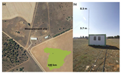
CO2 and CH4 dry concentrations were measured with a Picarro G1301 analyser that uses the cavity ring down spectroscopy technique. In this method, a laser beam describes a ring in a cavity. When the beam is turned off, the quantity and time of the decreasing signal at the detector depends on the gas concentration at the cavity. This analyser is located at the CIBA station, Low Atmosphere Research Centre (41°48′50″ N, 4°55′59″ W, 852 m a.s.l., Figure 1a) in the centre of the northern plateau of the Iberian Peninsula. Measurements were provided each 2–3 s. However, hourly means were calculated, and these values were used as initial observations for further calculations, such as monthly percentiles. The measurement campaign was extended over six years from 15 October 2010. Calibrations were made each two weeks with three standard concentrations prepared by the NOAA (National Oceanic and Atmospheric Administration), and measured concentrations were corrected following the calibration equations. Although measurements were considered at three levels (1.8 m, 3.7 m, and 8.3 m, Figure 1b), only the lowest was used in the current analysis, since differences among the observations were very low [16]. Following the Köppen Climate Classification, the climate at the site is Cfb, and it is temperate with a dry season and a temperate summer [17]. Vegetation comprises Mediterranean shrubland that develops mainly in spring and dies or sheds its leaves in summer. However, evergreen shrubs, such as thyme, are also present. Moreover, some rainfed crops are found in the surrounding areas.
2.2. Statistics
Monthly percentiles were calculated and fitted to linear equations, which were used to detrend the percentiles. Different statistics were calculated to describe the residuals. These statistics include the location indicator; the median of absolute values, the interquartile range (IQR)—in other words, the difference between the third and the first quartiles—which is used as a spread estimator, and the Yule–Kendall index (YK), which is a symmetry statistic [13],
where Q1, Q2, and Q3 are the first, second, and third quartiles, respectively.
YK = (Q1 + Q3 − 2Q2)/IQR
2.3. The lag-1 Autocorrelation as a Randomness Indicator
The concentration evolution is formed by two contributions, one of which is deterministic and the other random. By way of an example, let us suppose the function
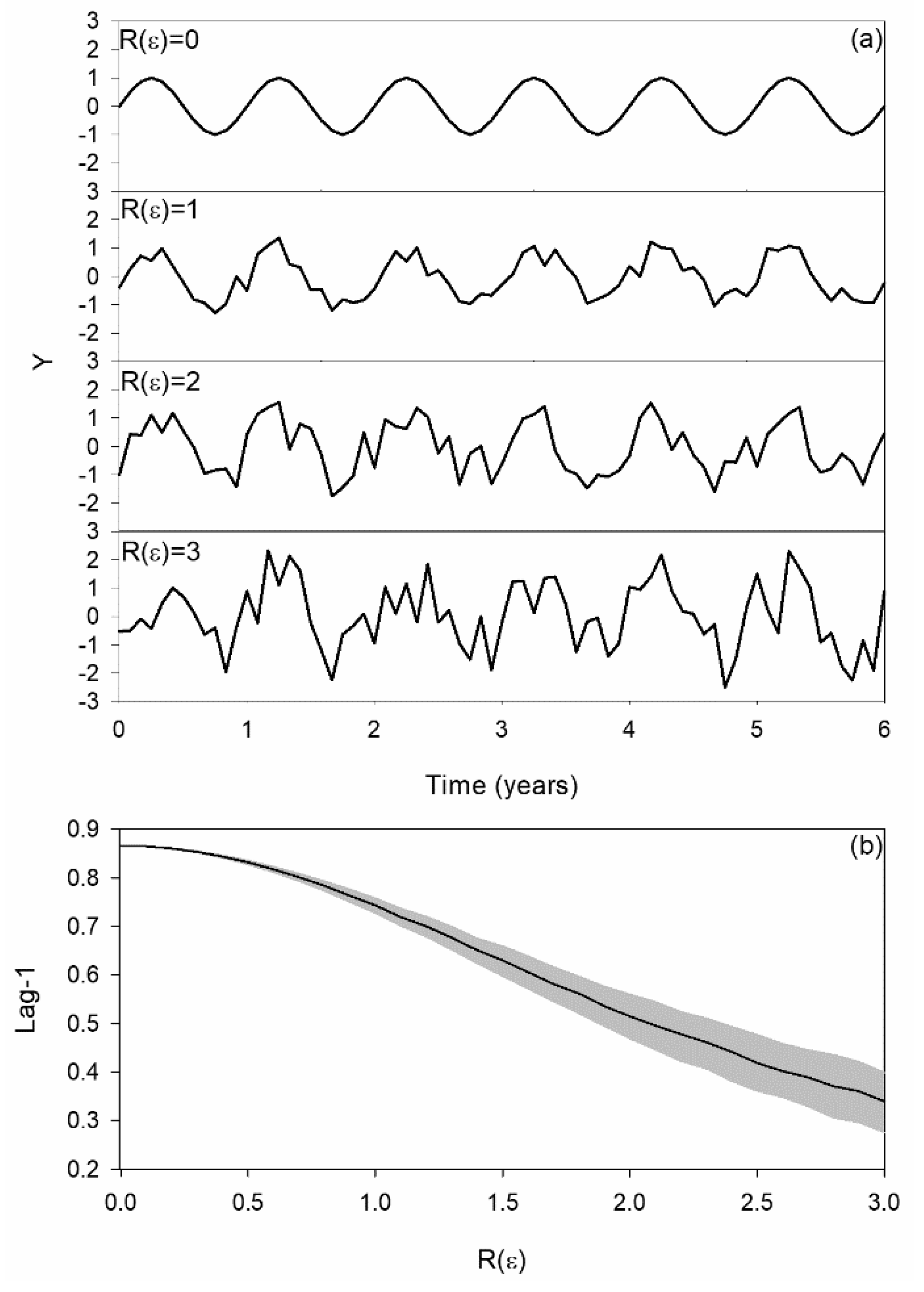
where t is the time in months and ε is a random variable uniformly distributed with an average null and variable range, R(ε), from 0 to 3, whose values are taken in 0.1 steps. Figure 2a presents Equation (2) with increasing values of R(ε). Small values of this range determine slight differences against the deterministic part of the function. However, large values of R(ε) hide this deterministic contribution.
Y = sin(2π/12 t) + ε
Time series analysis is a frequently used tool to investigate variables that display periodic behaviour. Methods such as Markov chains and autoregressive models have successfully been applied in this research line. The autocorrelation function has also been used in atmospheric research to provide information concerning time series persistence [18]. Recently, Anderson and Gough [19] considered the lag-1 autocorrelation when studying the influence of the previous value on the current one. Moreover, since this correlation coefficient, r, depends on the values of the random variable ε, Equation (2) was calculated 1000 times in the six-year period, and the lag-1 autocorrelation was obtained with each series. Figure 2b represents the quartiles of r for the lag-1 as a function of R(ε). Small values of this range are linked with the “memory” of the deterministic contribution of Equation (2). However, when R(ε) increases, r drops to low values, revealing a “memory loss” due to the increasing weight of the random part of Equation (2).
2.4. Harmonic Composition
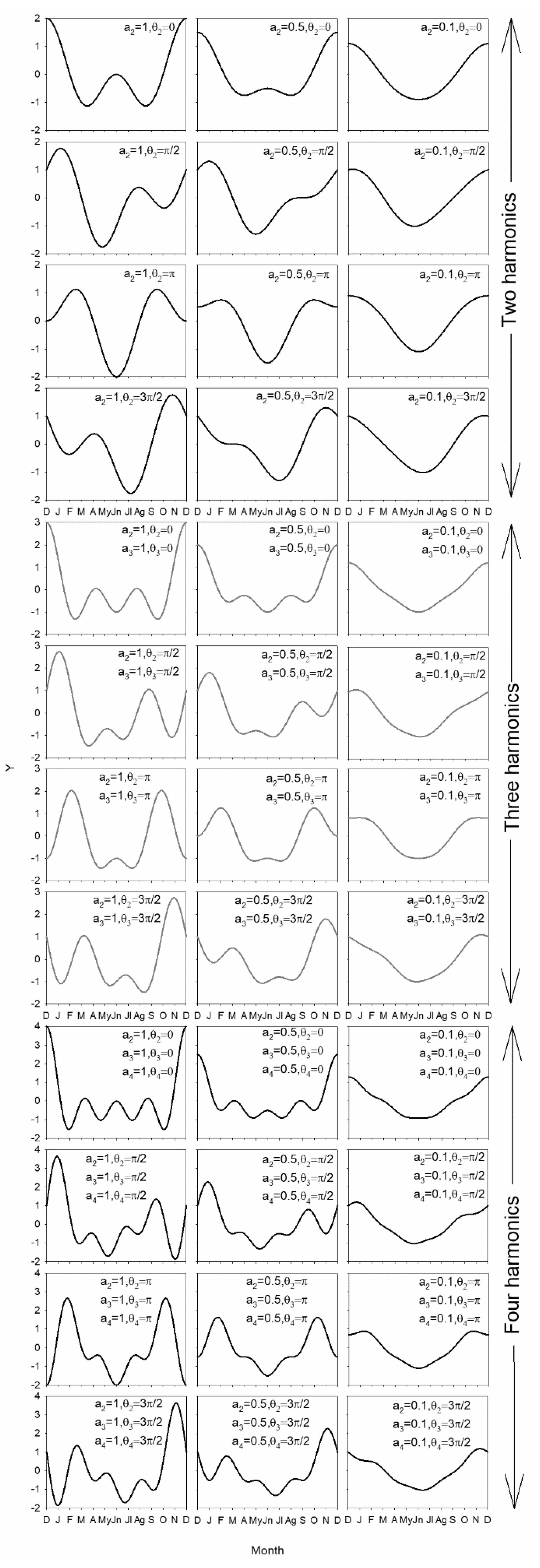
Following [20,21,22], let us consider the function formed by the addition of two harmonics,
where y is the concentration, T1 and T2 are periods established for both harmonics, and t is the time in months. Its coefficients may be fitted by multiple linear regression. In particular, the addition of two harmonics, one with an annual cycle, T1 = 12 months, an amplitude equal to one, a1 = 1 and a phase constant equal to zero, θ1 = 0, and the second with a semi-annual cycle, although with a different amplitude and phase constant, which provides the result presented in Figure 3.
y = a0 + a1 cos(2π/T1 t − θ1) + a2 cos(2π/T2 t − θ2)
The third and fourth harmonics (ai cos(2π/Ti t − θi), where T3 = 4 months for the third harmonic and T4 = 3 months for the fourth harmonic) were also added to Equation (3), and its response against specific values of the parameters is also presented in Figure 3.
3. Results
3.1. Evolution of Monthly Percentiles
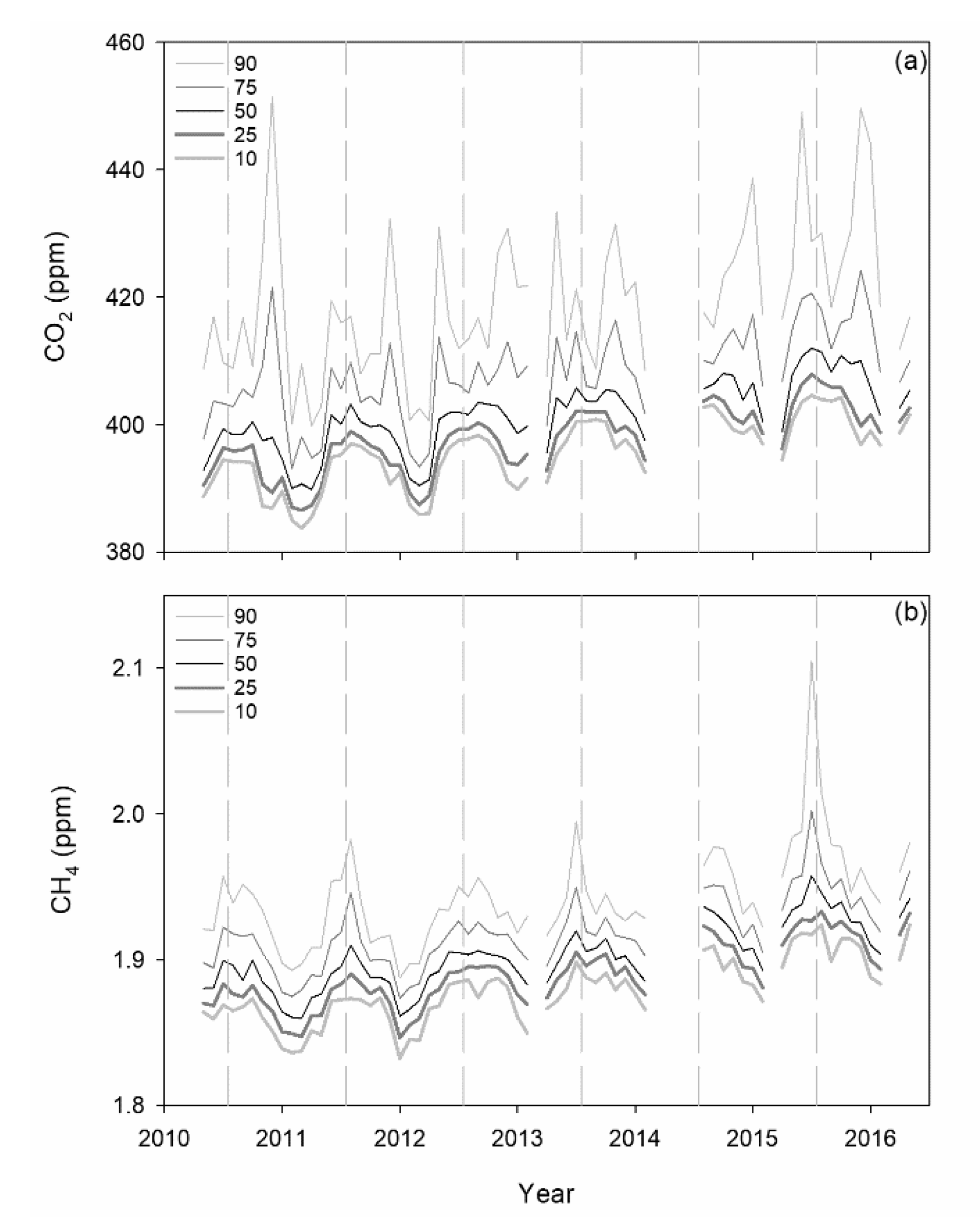
Percentiles were calculated with monthly observations in order to explore their evolution. Figure 4 presents the results for selected percentiles. The period considered is short enough to consider that it may be successfully described by a linear evolution. However, irregular shapes are obtained for extreme percentiles, especially for the highest, where the greatest outliers occasionally determine noticeable concentrations. Although outliers are also present in the low percentiles, their influence is less marked than in the high percentiles.
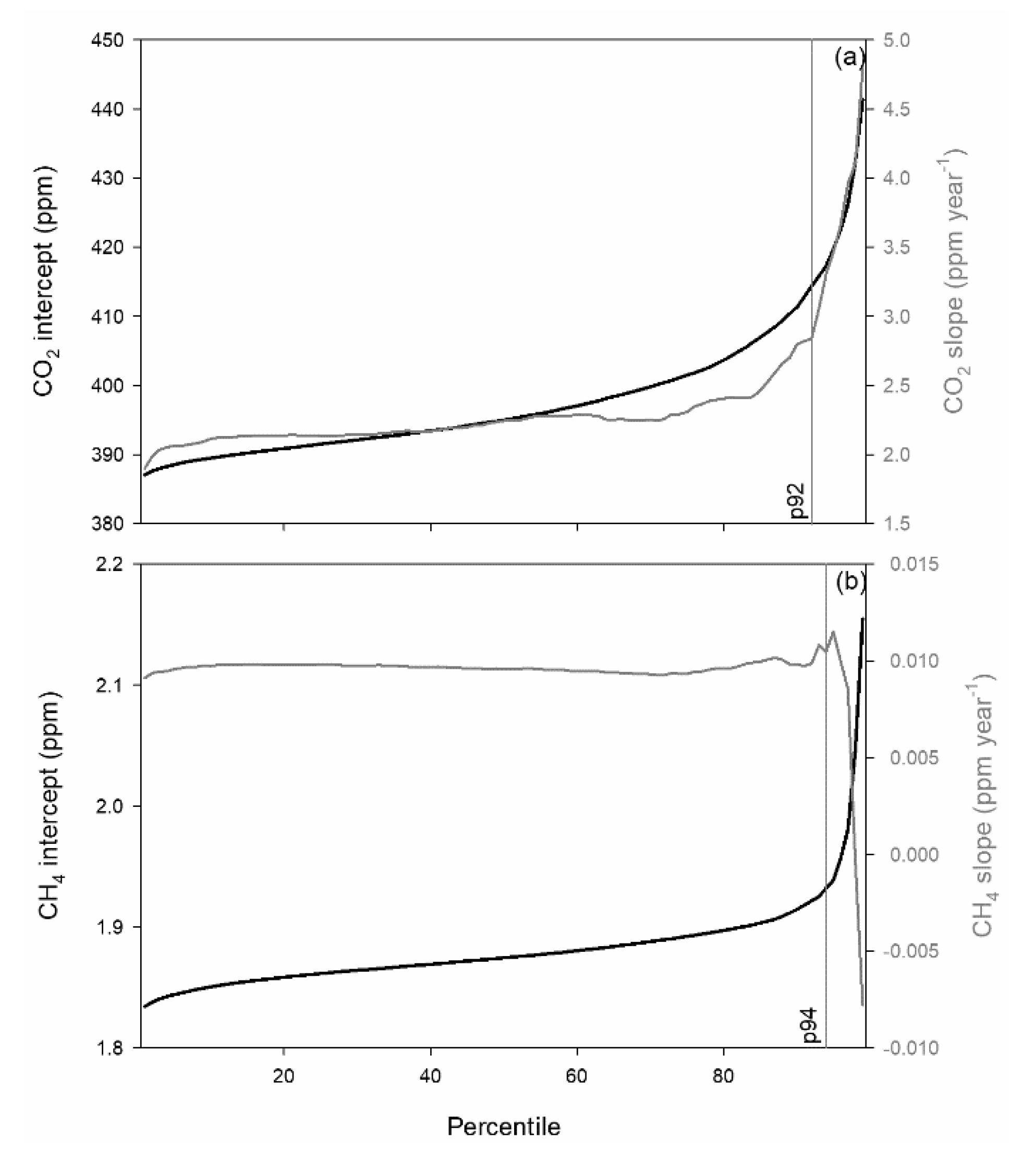
Linear regressions were calculated for percentiles. Intercepts and slopes are presented in Figure 5. Moreover, limits under which correlations are statistically significant at a 0.001 level are marked. Intercepts increase from 387.06 to 412.82 ppm for CO2 and from 1.8343 and 1.9251 ppm for CH4. However, slopes are steadier, around 2.24 ppm year−1 for CO2 and 0.0097 ppm year−1 for CH4 below the percentiles marked.
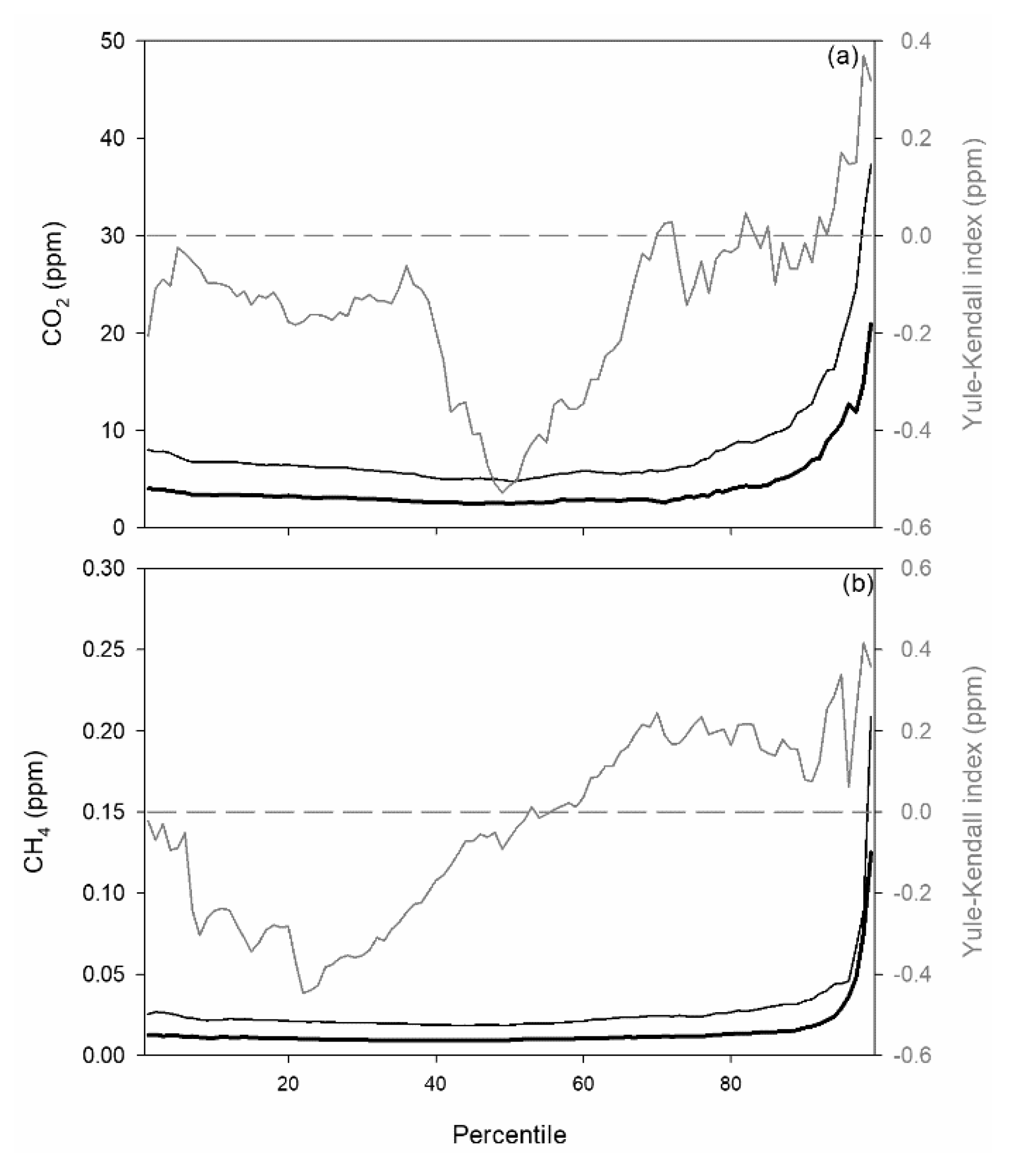
Monthly percentiles were detrended, and robust statistics of residuals (i.e., differences from the linear regression) introduced above were calculated and presented in Figure 6. Below the 80th percentile, the medians of the absolute value and the interquartile range of the residuals is very similar, around 3 and 6 ppm, respectively, for CO2 and around 0.01 and 0.02 ppm, respectively, for CH4. The Yule–Kendall index of residuals was negative for most percentiles, particularly between the 40th and 70th percentiles for CO2. However, this index was negative below the 50th percentile for CH4 residuals.
3.2. Lag-1 Autocorrelation
The lag-1 autocorrelation was calculated for the time series of monthly percentiles and presented in Figure 7. Moreover, Δ lag-1 for a specific percentile was calculated as the difference between lag-1 autocorrelation for the following percentile and this value for the preceding percentile. This quantity was used as an indicator of the change in the lag-1 autocorrelation with the percentile. Varied groups of percentiles were suggested following both the lag-1 autocorrelation and Δ lag-1. Five groups were proposed for CO2, where the first corresponds to an increase in the lag-1 autocorrelation. This value is steady in the second group. However, it decreases in the third group and at a greater rate in the fourth, where oscillations of Δ lag-1 were also noticeable. Finally, the last group was associated with major changes in Δ lag-1. Six groups of percentiles were suggested for CH4, where the first group features fast oscillations of Δ lag-1. These oscillations were wider in the second group. The lag-1 autocorrelation was steady in the third group and decreased slowly in the fourth. This decrease is more pronounced in the fifth group and is very sharp in the sixth.
3.3. Annual Cycle
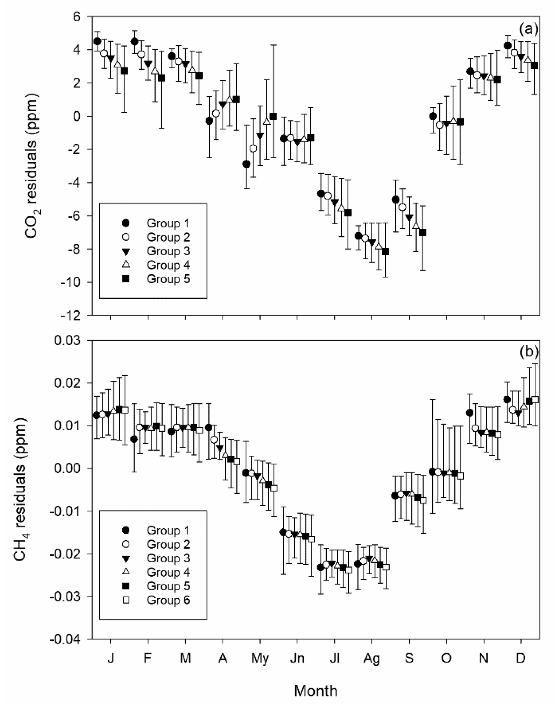
The initial observations were divided into the groups presented in Figure 7 and were detrended. Table 1 presents the parameters of linear fits. Correlation coefficients are high for central groups, but especially low for group 5 of CO2 and group 6 of CH4. Residuals were used to establish the annual cycle. Figure 8 presents the monthly medians and interquartile ranges for each group. The annual cycle is similar for both gases, since a high concentration is observed in winter and low values are reached in summer. However, groups 1 and 2 present a second minimum in May (which is more visible in Figure 9) that is not observed in the remaining groups for CO2. Moreover, the decrease in spring is slow, and the increase in autumn is fast. The behaviour of groups is similar for CH4, since interquartile ranges and skewnesses are nearly the same. However, both statistics depend on the group and month for CO2. The interquartile range increases from group 1 to 5 and, for group 5, skewness is mainly negative in January and February, but it is noticeably positive in May.
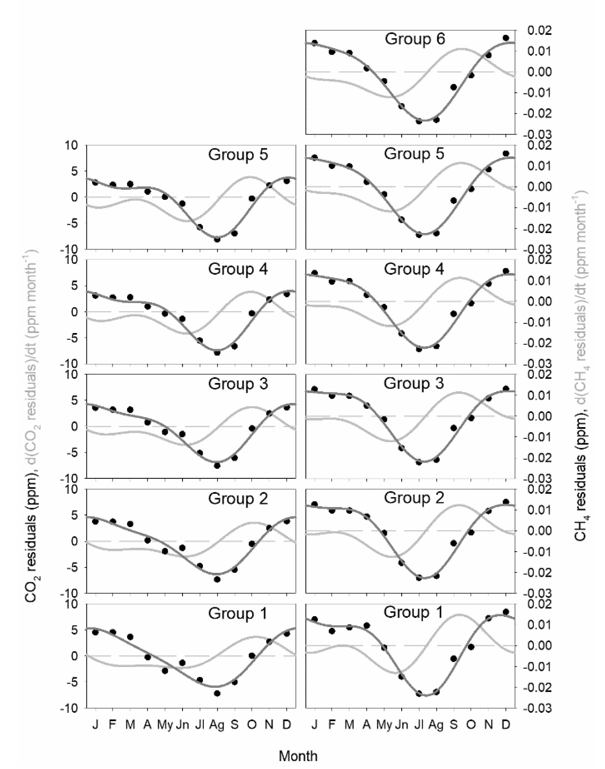
Some combinations of four harmonics have been suggested to fit the monthly medians of the groups formed. A look at the correlation coefficients in Table 2 reveals that the contribution of the fourth harmonic is extremely weak, with the third harmonic contribution being slightly better in general. As a result, the composition of annual and semi-annual cycles provides satisfactory agreement, since the inclusion of higher harmonics complicates the equation unnecessarily. The parameters of Equation (3) are presented in Table 3. The semi-annual amplitude is considerably lower than the annual amplitude for both gases. For CO2, the annual amplitude decreases when the percentile increases, although the semi-annual amplitude increases. Moreover, annual maxima are obtained in January–February, although semi-annual maxima are present around April–May and October–November. For CH4, the semi-annual amplitude decreases when the percentile increases. Annual maxima are obtained around January, although semi-annual maxima are calculated in March–September. The addition of the two harmonics produces the irregular evolution shown in Figure 9, where the derivative with respect to time is also presented for a better description of the evolution. The concentration of the two gases increases from August to December. However, two types of decrease were observed from January to August, particularly for CO2. The decrease is gradual for groups 1 and 2, since the derivative of concentration with respect to time is steady. However, one maximum close to zero is noticeable in March–April, revealing a step in concentration, which is slight for group 3, but more marked in groups 4 and 5. The opposite behaviour emerges for CH4, since this step of the concentration is marked for group 1, but gradually decreases from group 2 to group 6.
4. Discussion
4.1. Observations and Outliers
Pérez et al. [23] highlighted the different behaviour of selected percentiles and studied decile trends. The analysis presented in the current study expands that research by using all the percentiles. Although most of the measurements follow the evolution given by the trend and the yearly cycle [24], outliers are frequently observed due to local sources or sinks and transport from cities [25]. The shape of the annual cycle and the distribution of outliers are specific to the site. Figure 4 presents an annual cycle with low marked minima in summer for both gases when hemispheric CO2 uptake draws down global CO2 concentrations and CH4 is oxidised by OH throughout the hemisphere, although with noticeable outliers in spring for CO2 attributed to respiration when soils start to warm up but are still moist and vegetation develops, with low dispersion at night when atmospheric stable stratification prevails [26]. Moreover, outliers were frequent in winter for CH4 when the occasional impact of the Valladolid urban plume has also been reported [27]. This plume may be noticeably affected by natural gas heating during winter months and might contribute to CH4 outliers during stable stratification periods. However, hourly concentrations at Sammaltunturi, Finland, described by Lohila et al. [28] showed one very marked minimum in summer for CO2 and frequent high outliers for CH4 throughout the year. Higuchi et al. [29] studied CO2 at Fraserdale, Canada, where a noticeable range in the daily cycle was observed in summer. This pattern was also presented by Zhu and Yoshikawa-Inoue [30] at Rishiri Island in northern Japan. Frequent night-time outliers were attributed to the formation of stable boundary layers in this period together with plant and soil respiration. However, outliers of low CO2 daily means were measured in summer at Takayama, in central Japan [31]. Different behaviour was observed at Minamitorishima, a remote coral island in the western North Pacific, where few noticeable CO2 outliers were recorded [32].
4.2. Annual Trend
Liu et al. [33] considered an equation with a linear evolution for the trend accompanied by two sinusoidal terms and calculated its coefficients for CO2 in the period 1997–2006 following the vegetation classes from the International Geosphere-Biosphere Programme. They obtained a global value of 2.04 ppm year−1, which was slightly higher than that recorded at the Mauna Loa Observatory, with the highest trend being 4.92 ppm year−1 for open shrublands against no trend for grassland or mixed forest. The trend value closest to this study site was 2.28 ppm year−1 for the woody savannah, which responds to the steppe feature of the vegetation. The same equation was used by Wu et al. [34] for CO2 concentration at a tall forest in Northeast China in the period 2003–2010. They calculated 1.7 ppm year−1, which was close to the value presented by Liu et al. [33] for an evergreen needleleaf forest.
Vermeulen et al. [35] studied daily trimmed means of CO2 and CH4 among other gases at Cabaw, in the Netherlands, using an equation with a linear trend and four harmonics, and obtained an increase of 2.00 ppm year−1 for CO2 in the period 2005–2009 and 0.0074 ppm year−1 for CH4 in 2005–2010, which is slightly below those recorded in this research. Timokhina et al. [36] used the same equation for CO2 over central Siberia in the period 2006–2013 and obtained an increase of 2.02 ppm year−1 for CO2, which is similar to that of Vermeulen et al. [35]. Bergamaschi et al. [37] recorded a growth rate of around 0.004 ppm year−1 for CH4 in early 2010 in the Northern Hemisphere. Similarly, Dalsøren et al. [38] reported an increase in global mean surface CH4 of around 0.006 ppm year−1 in the period 1984–2012.
The low percentile trend is related with large-scale hemispheric and global background concentration evolution, whereas the high percentile trend is related with emission evolution. The results of this research agree with trends recorded at different observatories for low CO2 percentiles, with the CH4 trend for low percentiles being higher. However, the CO2 trend of high percentiles is greater than the low percentile trend, and it reveals the ever-increasing role played by CO2 emissions. The CH4 trend is similar for low and high percentiles, indicating that the emission contribution remains steady.
4.3. Harmonic Analysis
Equations with only the annual frequency, such as Liu et al. [33] or Wu et al. [34], who used an addition of two sinusoidal functions, respond to the simplest approach for explaining a near-symmetrical annual cycle. However, Figure 8 and Figure 9 reveal an asymmetrical evolution. Several harmonics have often been used to fit observations with enough detail. The most complex analyses consider four harmonics [35,36,39]. However, expressions with three harmonics have also been used [40,41,42]. As a result of this research, two harmonics may be considered as a suitable description of the annual cycle, which is in agreement with previous studies [20,21,22]. In fact, addition of the first and second harmonics has proved to be a suitable procedure to describe cycles with one maximum and one minimum that are unevenly distributed, such as the daily temperature cycle [43]. One result to emerge from the current paper is the extension of this procedure to explain the annual evolution of CO2 and CH4.
4.4. Annual Cycle
The contrast among latitudes and the time evolution of the two gases has been described by the NOAA [44]. Pu et al. [45] presented the CO2 annual cycle at Mauna Loa, Hawaii, which shows a very smooth evolution with one maximum in May and one minimum in September–October. The annual range was slightly higher at Waliguan, China, another remote station, although the maximum was observed in April and the minimum was observed in July–August. This latter evolution was similar to that observed at Jungfraujoch, Switzerland [46].
A similar cycle to that observed in this study was reported by Haszpra et al. [47], whose CO2 annual cycle at Hegyhátsál, Hungary, reflected a rapid increase from August to December, whereas the decrease in the rest of the year was slower, with a slight step in concentration in spring. However, the range was considerably higher, around 30 ppm. The low annual range at the CIBA station compared to other observatories was also described by Curcoll et al. [48] and could be explained by the weak influence of the sparse vegetation at this site. Hatakka et al. [49] presented the annual CO2 cycle in Pallas, northern Finland, where the concentration was highest in late winter and could be attributed to ecosystem respiration and the accumulation of this gas in the low atmosphere during this season. Similar cycles were presented by Higuchi et al. [29] for Fraserdale, Canada, with one maximum in April and one minimum in August; Alert, near the North Pole, where the annual cycle range was smaller and the maximum and minimum were delayed by approximately one month, and Cold Bay, Alaska, where the cycle was softer. Xia et al. [50] showed the CO2 annual cycle at the Lin’an regional background station, some 150 km from Shanghai, China, where a step in spring similar to that presented in Figure 9 for the highest percentiles may be observed. Fang et al. [51] presented the annual CO2 cycles at the same station, with different filtering procedures. The result was similar to that presented in Figure 9, although with a higher range and where the spring step depends on the filtering procedure followed.
With regard to CH4, Zhang et al. [52] compared the seasonal cycle among four observatories. Although two presented similar evolutions to those shown in this research, the seasonal cycle proved to be irregular for Zugspitze/Schneefernerhaus, southern Germany, with maxima in April and August, while the cycle at Waliguan, China, featured one maximum in summer.
Graven et al. [53] studied CO2 seasonal amplitude change following the latitude in the Northern Hemisphere. They observed that CO2 seasonal amplitude increases with latitude and with time above 35° N. However, the shape of the annual evolution may be affected by local features, which is a topic that is currently subject to inquiry [54].
5. Conclusions
A six-year CO2 and CH4 measurement campaign was carried out at the CIBA station, which is a site near a steppe with a slight urban influence located in the centre of the upper Spanish plateau.
The structure of the low atmosphere has a marked impact on CO2 and CH4 outliers at this rural site, since they are mainly observed at night when the low atmosphere is stably stratified. High CO2 values were observed in spring due to ecosystem respiration, whereas CH4 outliers were observed in winter, when the boundary layer height was low.
Since concentration evolution is slow in the six-year period analysed, linear equations are suitable to describe the trend. Most of the monthly percentiles provided similar annual rates, and residuals are low.
The lag-1 autocorrelation applied to monthly percentiles evidenced the contrast not only between outliers and regular observations, but also between the lowest and the highest concentrations. Five groups of observations were proposed for CO2 where the highest trend was observed for the highest percentiles, whereas six groups were proposed for CH4 with the highest trend below the 42nd percentile, i.e., for intermediate and small observations.
The annual cycle of residuals was similar for both trace gases, with a marked minimum in summer, and with group behaviour being similar for CH4. However, one concentration step in monthly medians was observed not only for high CO2 percentiles, but also for low CH4 percentiles. Harmonic analysis applied to these monthly medians revealed that annual and semi-annual harmonics satisfactorily described the seasonal evolution, with additional harmonics proving unnecessary.
Finally, the current research presents and applies a procedure to mark outliers and to examine how they impact average CO2 and CH4 concentrations and trends, which may be extended to other ecosystems and environments. Moreover, although the number of harmonics was set at two, further research around the cycle amplitude in the evolution equation is still open to detailed analysis at this site.
Author Contributions
Conceptualization, formal analysis and writing, I.A.P.; investigation, M.Á.G. and N.P.; review and editing, B.F.-D.; project administration and funding acquisition, M.L.S. All authors have read and agree to the published version of the manuscript.
Funding
This research was funded by The Ministry of Economy and Competitiveness and ERDF funds, project numbers CGL-2009-11979 and CGL2014-53948-P, and by the Regional Government of Castile and Leon, project number VA027G19.
Conflicts of Interest
The authors declare no conflict of interest. The funders had no role in the design of the study, in the collection, analyses, or interpretation of data, in the writing of the manuscript, or in the decision to publish the results.
References
- Fang, S.X.; Zhou, L.X.; Masarie, K.A.; Xu, L.; Rella, C.W. Study of atmospheric CH4 mole fractions at three WMO/GAW stations in China. J. Geophys. Res. Atmos. 2013, 11, 4874–4886. [Google Scholar] [CrossRef]
- Imasu, R.; Tanabe, Y. Diurnal and seasonal variations of carbon dioxide (CO2) concentration in urban, suburban, and rural areas around Tokyo. Atmosphere 2018, 9, 367. [Google Scholar] [CrossRef] [Green Version]
- Liu, L.; Zhou, L.; Zhang, X.; Wen, M.; Zhang, F.; Yao, B.; Fang, S. The characteristics of atmospheric CO2 concentration variation of four national background stations in China. Sci. China Ser. D-Earth Sci. 2009, 52, 1857–1863. [Google Scholar] [CrossRef]
- Liu, L.X.; Zhou, L.X.; Vaughn, B.; Miller, J.B.; Brand, W.A.; Rothe, M.; Xia, L.J. Background variations of atmospheric CO2 and carbon-stable isotopes at Waliguan and Shangdianzi stations in China. J. Geophys. Res. Atmos. 2014, 119, 5602–5612. [Google Scholar] [CrossRef]
- Fang, S.X.; Zhou, L.X.; Tans, P.P.; Ciais, P.; Steinbacher, M.; Xu, L.; Luan, T. In situ measurement of atmospheric CO2 at the four WMO/GAW stations in China. Atmos. Chem. Phys. 2014, 14, 2541–2554. [Google Scholar] [CrossRef] [Green Version]
- Kilkki, J.; Aalto, T.; Hatakka, J.; Portin, H.; Laurila, T. Atmospheric CO2 observations at Finnish urban and rural sites. Boreal Environ. Res. 2015, 20, 227–242. [Google Scholar]
- Fang, S.X.; Luan, T.; Zhang, G.; Wu, Y.L.; Yu, D.J. The determination of regional CO2 mole fractions at the Longfengshan WMO/GAW station: A comparison of four data filtering approaches. Atmos. Environ. 2015, 116, 36–43. [Google Scholar] [CrossRef]
- Zhang, F.; Fukuyama, Y.; Wang, Y.; Fang, S.; Li, P.; Fan, T.; Zhou, L.; Liu, X.; Meinhardt, F.; Emiliani, P. Detection and attribution of regional CO2 concentration anomalies using surface observations. Atmos. Environ. 2015, 123, 88–101. [Google Scholar] [CrossRef]
- Satar, E.; Berhanu, T.A.; Brunner, D.; Henne, S.; Leuenberger, M. Continuous CO2/CH4/CO measurements (2012-2014) at Beromunster tall tower station in Switzerland. Biogeosciences 2016, 13, 2623–2635. [Google Scholar] [CrossRef] [Green Version]
- Brailsford, G.W.; Stephens, B.B.; Gomez, A.J.; Riedel, K.; Mikaloff Fletcher, S.E.; Nichol, S.E.; Manning, M.R. Long-term continuous atmospheric CO2 measurements at Baring Head, New Zealand. Atmos. Meas. Tech. 2012, 5, 3109–3117. [Google Scholar] [CrossRef] [Green Version]
- Wang, Y.; Munger, J.W.; Xu, S.; McElroy, M.B.; Hao, J.; Nielsen, C.P.; Ma, H. CO2 and its correlation with CO at a rural site near Beijing: Implications for combustion efficiency in China. Atmos. Chem. Phys. 2010, 10, 8881–8897. [Google Scholar] [CrossRef] [Green Version]
- Stephens, B.B.; Brailsford, G.W.; Gomez, A.J.; Riedel, K.; Mikaloff Fletcher, S.E.; Nichol, S.; Manning, M. (2013) Analysis of a 39-year continuous atmospheric CO2 record from Baring Head, New Zealand. Biogeosciences 2013, 10, 2683–2697. [Google Scholar] [CrossRef] [Green Version]
- Wilks, D.S. Statistical Methods in the Atmospheric Sciences, 4th ed.; Elsevier: Amsterdam, The Netherlands, 2019. [Google Scholar]
- Fang, S.; Tans, P.P.; Steinbacher, M.; Zhou, L.; Luan, T.; Li, Z. Observation of atmospheric CO2 and CO at Shangri-La station: Results from the only regional station located at southwestern China. Tellus B 2016, 68, 28506. [Google Scholar] [CrossRef] [Green Version]
- van der Laan, S.; van der Laan-Luijkx, I.T.; Rödenbeck, C.; Varlagin, A.; Shironya, I.; Neubert, R.E.M.; Ramonet, M.; Meijer, H.A.J. Atmospheric CO2, δ(O2/N2), APO and oxidative ratios from aircraft flask samples over Fyodorovskoye, Western Russia. Atmos. Environ. 2014, 97, 174–181. [Google Scholar] [CrossRef]
- Pérez, I.A.; Sánchez, M.L.; García, M.A.; Pardo, N. Analysis and fit of surface CO2 concentrations at a rural site. Environ. Sci. Pollut. Res. 2012, 19, 3015–3027. [Google Scholar] [CrossRef]
- ITACYL—AEMET. Atlas Agroclimático de Castilla y León. Available online: http://atlas.itacyl.es (accessed on 4 March 2020).
- Pérez, I.A.; García, M.A.; Sánchez, M.L.; de Torre, B. Autocorrelation analysis of meteorological data from a RASS sodar. J. Appl. Meteorol. 2004, 43, 1213–1223. [Google Scholar] [CrossRef]
- Anderson, C.I.; Gough, W.A. Accounting for missing data in monthly temperature series: Testing rule-of-thumb omission of months with missing values. Int. J. Climatol. 2018, 38, 4990–5002. [Google Scholar] [CrossRef] [Green Version]
- Artuso, F.; Chamard, P.; Piacentino, S.; Sferlazzo, D.M.; De Silvestri, L.; di Sarra, A.; Meloni, D.; Monteleone, F. Influence of transport and trends in atmospheric CO2 at Lampedusa. Atmos. Environ. 2009, 43, 3044–3051. [Google Scholar] [CrossRef]
- Chamard, P.; Thiery, F.; Di Sarra, A.; Ciattaglia, L.; De Silvestri, L.; Grigioni, P.; Monteleone, F.; Piacentino, S. Interannual variability of atmospheric CO2 in the Mediterranean: Measurements at the island at Lampedusa. Tellus B 2003, 55, 83–93. [Google Scholar] [CrossRef]
- Cundari, V.; Colombo, T.; Ciattaglia, L. Thirteen years of atmospheric carbon dioxide measurements at Mt. Cimone station, Italy. Nuovo Cimento Soc. Ital. Fis. C 1995, 18, 33–47. [Google Scholar] [CrossRef]
- Pérez, I.A.; Sánchez, M.L.; García, M.A.; Pardo, N.; Fernández-Duque, B. The influence of meteorological variables on CO2 and CH4 trends recorded at a semi-natural station. J. Environ. Manage. 2018, 209, 37–45. [Google Scholar] [CrossRef] [PubMed] [Green Version]
- Pérez, I.A.; Sánchez, M.L.; García, M.A.; Pardo, N. Trend analysis of CO2 and CH4 recorded at a semi-natural site in the northern plateau of the Iberian Peninsula. Atmos. Environ. 2017, 151, 24–33. [Google Scholar] [CrossRef] [Green Version]
- Fang, S.X.; Tans, P.P.; Dong, F.; Zhou, H.; Luan, T. Characteristics of atmospheric CO2 and CH4 at the Shangdianzi regional background station in China. Atmos. Environ. 2016, 131, 1–8. [Google Scholar] [CrossRef]
- Ayalneh Berhanu, T.; Satar, E.; Schanda, R.; Nyfeler, P.; Moret, H.; Brunner, D.; Oney, B.; Leuenberger, M. Measurements of greenhouse gases at Beromünster tall-tower station in Switzerland. Atmos. Meas. Tech. 2016, 9, 2603–2614. [Google Scholar] [CrossRef] [Green Version]
- Pérez, I.A.; Sánchez, M.L.; García, M.A.; de Torre, B. CO2 transport by urban plumes in the upper Spanish plateau. Sci. Total Environ. 2009, 407, 4934–4938. [Google Scholar] [CrossRef] [PubMed]
- Lohila, A.; Penttilä, T.; Jortikka, S.; Aalto, T.; Anttila, P.; Asmi, E.; Aurela, M.; Hatakka, J.; Hellén, H.; Henttonen, H.; et al. Preface to the special issue on integrated research of atmosphere, ecosystems and environment at Pallas. Boreal Environ. Res. 2015, 20, 431–454. [Google Scholar]
- Higuchi, K.; Worthy, D.; Chan, D.; Shashkov, A. Regional source/sink impact on the diurnal, seasonal and inter-annual variations in atmospheric CO2 at a boreal forest site in Canada. Tellus B 2003, 55, 115–125. [Google Scholar] [CrossRef]
- Zhu, C.; Yoshikawa-Inoue, H. Seven years of observational atmospheric CO2 at a maritime site in northernmost Japan and its implications. Sci. Total Environ. 2015, 524, 331–337. [Google Scholar] [CrossRef]
- Murayama, S.; Saigusa, N.; Chan, D.; Yamamoto, S.; Kondo, H.; Eguchi, Y. Temporal variations of atmospheric CO2 concentration in a temperate deciduous forest in central Japan. Tellus B 2003, 55, 232–243. [Google Scholar] [CrossRef]
- Wada, A.; Sawa, Y.; Matsueda, H.; Taguchi, S.; Murayama, S.; Okubo, S.; Tsutsumi, Y. Influence of continental air mass transport on atmospheric CO2 in the western North Pacific. J. Geophys. Res.-Atmos. 2007, 112, D07311. [Google Scholar] [CrossRef]
- Liu, M.; Wu, J.; Zhu, X.; He, H.; Jia, W.; Xiang, W. Evolution and variation of atmospheric carbon dioxide concentration over terrestrial ecosystems as derived from eddy covariance measurements. Atmos. Environ. 2015, 114, 75–82. [Google Scholar] [CrossRef] [Green Version]
- Wu, J.; Guan, D.; Yuan, F.; Yang, H.; Wang, A.; Jin, C. Evolution of atmospheric carbon dioxide concentration at different temporal scales recorded in a tall forest. Atmos. Environ. 2012, 61, 9–14. [Google Scholar] [CrossRef]
- Vermeulen, A.T.; Hensen, A.; Popa, M.E.; van den Bulk, W.C.M.; Jongejan, P.A.C. Greenhouse gas observations from Cabauw Tall Tower (1992–2010). Atmos. Meas. Tech. 2011, 4, 617–644. [Google Scholar] [CrossRef] [Green Version]
- Timokhina, A.V.; Prokushkin, A.S.; Onuchin, A.A.; Panov, A.V.; Kofman, G.B.; Verkhovets, S.V.; Heimann, M. Long-term trend in CO2 concentration in the surface atmosphere over Central Siberia. Russ. Meteorol. Hydrol. 2015, 40, 186–190. [Google Scholar] [CrossRef]
- Bergamaschi, P.; Houweling, S.; Segers, A.; Krol, M.; Frankenberg, C.; Scheepmaker, R.A.; Dlugokencky, E.; Wofsy, S.C.; Kort, E.A.; Sweeney, C.; et al. Atmospheric CH4 in the first decade of the 21st century: Inverse modeling analysis using SCIAMACHY satellite retrievals and NOAA surface measurements. J. Geophys. Res. Atmos. 2013, 118, 7350–7369. [Google Scholar] [CrossRef] [Green Version]
- Dalsøren, S.B.; Myhre, C.L.; Myhre, G.; Gomez-Pelaez, A.J.; Søvde, O.A.; Isaksen, I.S.A.; Weiss, R.F.; Harth, C.M. Atmospheric methane evolution the last 40 years. Atmos. Chem. Phys. 2016, 16, 3099–3126. [Google Scholar] [CrossRef] [Green Version]
- Artuso, F.; Chamard, P.; Piacentino, S.; di Sarra, A.; Meloni, D.; Monteleone, F.; Sferlazzo, D.M.; Thiery, F. Atmospheric methane in the Mediterranean: Analysis of measurements at the island of Lampedusa during 1995-2005. Atmos. Environ. 2007, 41, 3877–3888. [Google Scholar] [CrossRef]
- Aalto, T.; Hatakka, J.; Paatero, I.; Tuovinen, J.P.; Aurela, M.; Laurila, T.; Holmén, K.; Trivett, N.; Viisanen, Y. Tropospheric carbon dioxide concentrations at a northern boreal site in Finland: Basic variations and source areas. Tellus B 2002, 54, 110–126. [Google Scholar] [CrossRef]
- Eneroth, K.; Aalto, T.; Hatakka, J.; Holmén, K.; Laurila, T.; Viisanen, Y. Atmospheric transport of carbon dioxide to a baseline monitoring station in northern Finland. Tellus B 2005, 57, 366–374. [Google Scholar] [CrossRef]
- Inoue, H.Y.; Matsueda, H.; Igarashi, Y.; Sawa, Y.; Wada, A.; Nemoto, K.; Sartorius, H.; Schlosser, C. Seasonal and long-term variations in atmospheric CO2 and 85Kr in Tsukuba, central Japan. J. Meteor. Soc. Jpn. 2006, 84, 959–968. [Google Scholar] [CrossRef] [Green Version]
- Wang, K.; Li, Y.; Wang, Y.; Yang, X. On the asymmetry of the urban daily air temperature cycle. J. Geophys. Res. 2017, 122, 5625–5635. [Google Scholar] [CrossRef]
- Available online: https://www.esrl.noaa.gov/gmd/ccgg/gallery/figures/ (accessed on 29 June 2020).
- Pu, J.J.; Xu, H.H.; He, J.; Fang, S.X.; Zhou, L.X. Estimation of regional background concentration of CO2 at Lin’an Station in Yangtze River Delta, China. Atmos. Environ. 2014, 94, 402–408. [Google Scholar] [CrossRef]
- Uglietti, C.; Leuenberger, M.; Brunner, D. European source and sink areas of CO2 retrieved from Lagrangian transport model interpretation of combined O2 and CO2 measurements at the high alpine research station Jungfraujoch. Atmos. Chem. Phys. 2011, 11, 8017–8036. [Google Scholar] [CrossRef] [Green Version]
- Haszpra, L.; Barcza, Z.; Hidy, D.; Szilágyi, I.; Dlugokencky, E.; Tans, P. Trends and temporal variations of major greenhouse gases at a rural site in Central Europe. Atmos. Environ. 2008, 42, 8707–8716. [Google Scholar] [CrossRef]
- Curcoll, R.; Camarero, L.; Bacardit, M.; Àgueda, A.; Grossi, C.; Gacia, E.; Font, A.; Morguí, J.A. Atmospheric carbon dioxide variability at Aigüestortes, Central Pyrenees, Spain. Reg. Envir. Chang. 2019, 19, 313–324. [Google Scholar] [CrossRef] [Green Version]
- Hatakka, J.; Aalto, T.; Aaltonen, V.; Aurela, M.; Hakola, H.; Komppula, M.; Laurila, T.; Lihavainen, H.; Paatero, J.; Salminen, K.; et al. Overview of the atmospheric research activities and results at Pallas GAW station. Boreal Environ. Res. 2003, 8, 365–383. [Google Scholar]
- Xia, L.; Zhou, L.; Tans, P.P.; Liu, L.; Zhang, G.; Wang, H.; Luan, T. Atmospheric CO2 and its δ13C measurements from flask sampling at Lin’an regional background station in China. Atmos. Environ. 2015, 117, 220–226. [Google Scholar] [CrossRef]
- Fang, S.X.; Tans, P.P.; Steinbacher, M.; Zhou, L.X.; Luan, T. Comparison of the regional CO2 mole fraction filtering approaches at a WMO/GAW regional station in China. Atmos. Meas. Tech. 2015, 8, 5301–5313. [Google Scholar] [CrossRef] [Green Version]
- Zhang, F.; Zhou, L.X.; Xu, L. Temporal variation of atmospheric CH4 and the potential source regions at Waliguan, China. Sci. China Earth Sci. 2013, 56, 727–736. [Google Scholar] [CrossRef]
- Graven, H.D.; Keeling, R.F.; Piper, S.C.; Patra, P.K.; Stephens, B.B.; Wofsy, S.C.; Welp, L.R.; Sweeney, C.; Tans, P.P.; Kelley, J.J.; et al. Enhanced seasonal exchange of CO2 by Northern ecosystems since 1960. Science 2013, 341, 1085–1089. [Google Scholar] [CrossRef] [Green Version]
- Yuan, Y.; Ries, L.; Petermeier, H.; Trickl, T.; Leuchner, M.; Couret, C.; Sohmer, R.; Meinhardt, F.; Menzel, A. On the diurnal, weekly, and seasonal cycles and annual trends in atmospheric CO2 at Mount Zugspitze, Germany, during 1981–2016. Atmos. Chem. Phys. 2019, 19, 999–1012. [Google Scholar] [CrossRef] [Green Version]
Figure 1.
(a) PNOA (National Plan of Aerial Orthophotography) image courtesy of © ign.es showing the measurement site together with its location in Spain. (b) Analyser housing and measurement heights.
Figure 1.
(a) PNOA (National Plan of Aerial Orthophotography) image courtesy of © ign.es showing the measurement site together with its location in Spain. (b) Analyser housing and measurement heights.

Figure 2.
(a) Representation of Equation (2) with four selected ranges of the random variable ε. (b) Correlation coefficient for the lag-1 autocorrelation as a function of the range of the random variable ε. One thousand functions were proposed for each range. The median is presented in black, and the interquartile range is shown in grey.

Figure 3.
Representation of Equation (3) with a0 = 0, a1 = 1, θ1 = 0, T1 = 12 months, T2 = 6 months, and varied values of a2 and θ2, labelled as two harmonics. The addition of the third and fourth harmonics (T3 = 4 and T4 = 3 months) is also plotted.
Figure 3.
Representation of Equation (3) with a0 = 0, a1 = 1, θ1 = 0, T1 = 12 months, T2 = 6 months, and varied values of a2 and θ2, labelled as two harmonics. The addition of the third and fourth harmonics (T3 = 4 and T4 = 3 months) is also plotted.

Figure 4.
Selected percentiles calculated from monthly concentrations. (a) CO2, (b) CH4.

Figure 5.
Parameters of the linear fit of monthly percentiles. Vertical lines indicate that correlations below these percentiles are statistically significant at a 0.001 level. (a) CO2, (b) CH4.
Figure 5.
Parameters of the linear fit of monthly percentiles. Vertical lines indicate that correlations below these percentiles are statistically significant at a 0.001 level. (a) CO2, (b) CH4.

Figure 6.
Statistics of percentiles of detrended residuals. The lowest thick black line is the median of the absolute value, and the highest thin black line is the interquartile range. (a) CO2, (b) CH4. The Yule–Kendall index is the grey line.
Figure 6.
Statistics of percentiles of detrended residuals. The lowest thick black line is the median of the absolute value, and the highest thin black line is the interquartile range. (a) CO2, (b) CH4. The Yule–Kendall index is the grey line.

Figure 7.
Groups of percentiles following the lag-1 autocorrelation and Δ lag-1. (a) CO2, (b) CH4.

Figure 8.
Monthly medians and interquartile ranges of detrended observations distributed following the groups presented in Figure 7. (a) CO2, (b) CH4.
Figure 8.
Monthly medians and interquartile ranges of detrended observations distributed following the groups presented in Figure 7. (a) CO2, (b) CH4.

Figure 9.
Monthly medians in dots and fit of Equation (3) with coefficients from Table 3. Derivatives of these functions with respect to time are presented in light grey.
Figure 9.
Monthly medians in dots and fit of Equation (3) with coefficients from Table 3. Derivatives of these functions with respect to time are presented in light grey.


Table 1.
Linear trend parameters and their uncertainty (5% level) for groups of percentiles.
| Gas | Group | Intercept (ppm) | Slope (ppm year−1) | r |
|---|---|---|---|---|
| CO2 | 1 | 388.7 ± 0.2 | 2.00 ± 0.06 | 0.646 |
| 2 | 392.07 ± 0.12 | 2.12 ± 0.04 | 0.696 | |
| 3 | 395.83 ± 0.17 | 2.25 ± 0.05 | 0.693 | |
| 4 | 401.4 ± 0.2 | 2.33 ± 0.07 | 0.530 | |
| 5 | 418.3 ± 1.0 | 3.6 ± 0.3 | 0.263 | |
| CH4 | 1 | 1.8442 ± 0.0008 | 0.0092 ± 0.0003 | 0.710 |
| 2 | 1.8584 ± 0.0006 | 0.00950 ± 0.00018 | 0.769 | |
| 3 | 1.8673 ± 0.0006 | 0.00937 ± 0.00019 | 0.777 | |
| 4 | 1.8819 ± 0.0005 | 0.00890 ± 0.00015 | 0.685 | |
| 5 | 1.9061 ± 0.0010 | 0.0087 ± 0.0003 | 0.551 | |
| 6 | 2.016 ± 0.011 | 0.002 ± 0.003 | 0.019 * |
* Value not statistically significant at the 5% level.
Table 2.
Correlation coefficients for different harmonic compositions.
| Gas | Harmonic | Group | |||||
|---|---|---|---|---|---|---|---|
| 1 | 2 | 3 | 4 | 5 | 6 | ||
| CO2 | Annual | 0.894 | 0.885 | 0.871 | 0.830 | 0.796 | |
| Annual and semi-annual | 0.926 | 0.942 | 0.958 | 0.962 | 0.961 | ||
| Annual and 3rd | 0.952 | 0.932 | 0.906 | 0.860 | 0.827 | ||
| Annual, semi-annual, and 3rd | 0.985 | 0.989 | 0.993 | 0.992 | 0.991 | ||
| Annual and 4th | 0.906 | 0.893 | 0.875 | 0.832 | 0.797 | ||
| Annual, semi-annual, and 4th | 0.938 | 0.951 | 0.962 | 0.964 | 0.962 | ||
| CH4 | Annual | 0.840 | 0.895 | 0.910 | 0.922 | 0.932 | 0.936 |
| Annual and semi-annual | 0.972 | 0.981 | 0.979 | 0.978 | 0.978 | 0.978 | |
| Annual and 3rd | 0.855 | 0.904 | 0.920 | 0.930 | 0.939 | 0.942 | |
| Annual, semi-annual, and 3rd | 0.987 | 0.990 | 0.989 | 0.986 | 0.985 | 0.985 | |
| Annual and 4th | 0.843 | 0.898 | 0.914 | 0.930 | 0.942 | 0.946 | |
| Annual, semi-annual, and 4th | 0.975 | 0.984 | 0.983 | 0.986 | 0.988 | 0.989 | |
Table 3.
Parameters of Equation (3).
| Gas | Group | a0 (ppm) | a1 (ppm) | θ1 (month) | a2 (ppm) | θ2 (month) |
|---|---|---|---|---|---|---|
| CO2 | 1 | −0.16 | 5.29 | 1.3 | 1.00 | 11.3 |
| 2 | −0.35 | 5.03 | 1.5 | 1.28 | 10.9 | |
| 3 | −0.44 | 5.03 | 1.6 | 1.59 | 10.5 | |
| 4 | −0.59 | 4.95 | 1.7 | 1.98 | 10.4 | |
| 5 | −0.74 | 4.88 | 1.7 | 2.22 | 10.3 | |
| CH4 | 1 | −0.0002 | 0.0171 | 1.2 | 0.0068 | 9.1 |
| 2 | −0.0005 | 0.0169 | 1.2 | 0.0052 | 8.8 | |
| 3 | −0.0007 | 0.0166 | 1.2 | 0.0046 | 8.7 | |
| 4 | −0.0010 | 0.0171 | 1.2 | 0.0042 | 8.9 | |
| 5 | −0.0012 | 0.0178 | 1.1 | 0.0040 | 9.0 | |
| 6 | −0.0017 | 0.0181 | 1.1 | 0.0039 | 9.1 |
© 2020 by the authors. Licensee MDPI, Basel, Switzerland. This article is an open access article distributed under the terms and conditions of the Creative Commons Attribution (CC BY) license (http://creativecommons.org/licenses/by/4.0/).
Share and Cite
MDPI and ACS Style
Pérez, I.A.; Sánchez, M.L.; García, M.Á.; Pardo, N.; Fernández-Duque, B. Statistical Analysis of the CO2 and CH4 Annual Cycle on the Northern Plateau of the Iberian Peninsula. Atmosphere 2020, 11, 769. https://doi.org/10.3390/atmos11070769
AMA Style
Pérez IA, Sánchez ML, García MÁ, Pardo N, Fernández-Duque B. Statistical Analysis of the CO2 and CH4 Annual Cycle on the Northern Plateau of the Iberian Peninsula. Atmosphere. 2020; 11(7):769. https://doi.org/10.3390/atmos11070769
Chicago/Turabian StylePérez, Isidro A., M. Luisa Sánchez, M. Ángeles García, Nuria Pardo, and Beatriz Fernández-Duque. 2020. "Statistical Analysis of the CO2 and CH4 Annual Cycle on the Northern Plateau of the Iberian Peninsula" Atmosphere 11, no. 7: 769. https://doi.org/10.3390/atmos11070769
Note that from the first issue of 2016, this journal uses article numbers instead of page numbers. See further details here.