SSH-Aerosol v1.1: A Modular Box Model to Simulate the Evolution of Primary and Secondary Aerosols


1
CEREA, Joint laboratory École des Ponts ParisTech and EdF R&D, 77 455 Marne la Vallée, France
2
Institut National de l’Environnement Industriel et des Risques, INERIS, 60 550 Verneuil en Halatte, France
*
Author to whom correspondence should be addressed.
Atmosphere 2020, 11(5), 525; https://doi.org/10.3390/atmos11050525
Submission received: 8 April 2020
/
Revised: 15 May 2020
/
Accepted: 17 May 2020
/
Published: 20 May 2020
(This article belongs to the Special Issue Atmospheric Modeling Study)
Abstract
:Particles are emitted by different sources and are also formed in the atmosphere. Despite the large impact of atmospheric particles on health and climate, large uncertainties remain concerning their representation in models. To reduce these uncertainties as much as possible, a representation of the main processes involved in aerosol dynamics and chemistry is necessary. For that purpose, SSH-aerosol was developed to represent the evolution of the mass and number concentrations of primary and secondary particles, across different scales, using state-of-the-art modules, taking into account processes that are usually not considered in air-quality or climate modelling. For example, the particle mixing state and the growth of ultra-fine particles are taken into account in the aerosol dynamics, the affinity of semi-volatile organic compounds with water and viscosity are taken into account in the partitioning between the gas and particle phases of organics and the formation of extremely low-volatility organic compounds from biogenic precursors is represented. SSH-aerosol is modular and can be used with different levels of complexity. It may be used as standalone to analyse chamber measurements. It is also designed to be easily coupled to 3D models, adapting the level of complexity to the spatial scale studied.
1. Introduction
With the impact of air pollution on health and ecosystems being a great concern, models, such as chemical-transport models (CTM), are often used to simulate air quality, i.e., to compute the concentration of atmospheric gases, aqueous-phase species and particulate matter (PM). Particles, especially fine particles, lead to adverse effects on human health [1], as well as visibility reduction. They also affect the manner in which radiation passes through the atmosphere [2] and represent an uncertain component of climate changes due to direct and indirect effects on the Earth’s radiative budget. Particles are complex mixtures made of several compounds, and of size ranging from a few nanometres to several micrometres. They can be emitted directly from various sources (e.g., natural such as wild fires, sea-salt, dust and anthropogenic) or can be formed in the atmosphere from the transformations of organic or inorganic gas precursors. The aerosol dynamics is governed by condensation/evaporation of condensable compounds (semi-volatile compounds that can condense on particles), coagulation and nucleation. The underlying processes are particularly complex, and they may be represented using different approaches. Hence, several aerosol models have been developed [3,4,5,6,7,8,9,10,11,12,13,14,15,16]), either as box stand-alone models, or as coupled to a 3D model.
The SSH-aerosol model is based on the coupling of three state-of-the-art modules: SCRAM (Size-Composition Resolved Aerosol Model [17]) for the dynamic evolution, SOAP (Secondary Organic Aerosol Processor, [18]) for gas/particle partitioning of organic compounds and H2O (Hydrophobic/Hydrophilic Organics [19,20,21]) for the formation of condensable organic compounds.
1.1. Aerosol Dynamics
The PM size distribution may be modelled using different approaches, among which the most common ones in CTMs are the sectional size distribution (the size distribution is discretised into sections, e.g., [3,4,5,6,7,8,9,10]) and the modal size distribution (the size distribution is discretised into log-normal modes, e.g., [11,12,13,14]). Because Sartelet et al. [14], Devilliers et al. [22] showed that modal models have difficulties in dealing with the growth of ultra-fine particles, SCRAM uses a sectional approach. For 3D applications, because each section or mode is transported individually, the size range of each section or mode needs to be constant throughout the simulation. As particles grow/shrink with condensation/evaporation, the bounds of the sections evolve, and it is necessary to redistribute the number and mass on fixed section bounds, introducing numerical errors. Different approaches are implemented in SCRAM depending on whether the mean diameter of the section is allowed to vary or not [22].
In CTMs, internal mixing is often assumed, i.e., a chemical composition is associated to each particle size section [5,15,16,23,24,25]. Although this assumption may be appropriate for air masses far from emission sources, it may be unrealistic close to emission sources, where emitted particles can have compositions that are very different from background particles and from particles emitted from other sources. The mixing state is partially resolved in models (e.g., [12,26]) which consider particles to be either mixed or not mixed. In numerous climate models, the mixing state is often treated implicitly by using an ageing time to convert freshly emitted particles from externally to internally mixed [27]. The mixing state is explicitly resolved in SCRAM; both the particle size distribution and the mass fraction of chemical compounds inside particles are discretised into sections. In other words, the chemical composition of particles in each size section is discretised according to the percentage of one or more of its compounds, as detailed in [28]. A similar discretisation is performed for the percentage of black carbon in [10,29]. SCRAM was used to show that, over Greater Paris in summer, more than half (up to 80% during rush hours) of black carbon particles are barely mixed at the centre of Paris, while BC particles are more mixed outside [30]. Mixing-state resolved simulations show higher nitrate and lower ammonium concentrations in the particle phase than internal-mixing simulations, leading to differences up to 22% in inorganic concentrations, 80% in the water content of particles and 72% in aerosol optical depth [30].
1.2. Formation of Condensable
Secondary pollutants such as ozone (O3) and PM precursors are formed during the gas-phase degradation of anthropogenic and biogenic compounds: oxides of nitrogen and volatile organic compounds (VOCs). Because of its health impact and its link to the oxidation capacity of the atmosphere, the formation and destruction of O3 have been extensively studied, and different condensed chemical mechanisms have been developed: lumped structure mechanisms (CB05 [31]) and lumped species mechanisms (RACM2 [32] and SAPRC [33]).
As organic gases are oxidised in the gas phase (by OH, O3 and NO3), their volatility evolves. It may decrease by the addition of polar functional groups (such as hydroxyl, hydroperoxyl, nitrate and acid groups). On the other hand, some oxidation products may have higher volatility than the parent organic gases due to the cleavage of carbon–carbon bonds. Products of low volatility may condense on the available particles to establish equilibrium between the gas and particle phases. The formation of these semi-volatile organic species (SVOC) is often not considered in the mechanisms described previously, which were originally developed to model O3 concentrations. To be able to represent SOA formation using these models, additional oxidation products corresponding to surrogate SVOC species are added to most 3D models using different approaches [19,34,35], as now detailed.
Due to the lack of knowledge and the sheer number and complexity of organic species, most chemical reaction schemes for organics are very crude representations of the true mechanism. Different categories of SOA models exist: the widely used two-compound Odum approach [36] and the more recent volatility basis set (VBS) approach [35,37,38]. H2O represents the formation of SOA using surrogate molecules with representative physico-chemical properties for gas/particle partitioning [19]. This approach allows us to take into account the most relevant processes for SOA formation (completeness of the precursor VOC list [21], ideality assumption, treatment of oligomerization, importance of low-NOx vs. high-NOx regimes and treatment of SOA affinity with water) [39]. Although only a few surrogates are used to represent the SOA formation, the oxidation properties and the affinity with water of organic particles are well represented in the H2O model by comparison to measurements made in the south of France (Europe) in summer, when the biogenic contribution to SOA is important Chrit et al. [20], Freney et al. [40]. However, in winter time, when the anthropogenic contribution of SOA is dominant, both the surrogate and the VBS approaches underestimate the oxidation degree of SOA [41]. The SOA affinity with water, which is often ignored in 3D models [15,16,35], largely influences the formation of organic aerosols. The measurements of Chrit et al. [20] showed that about 64% of the organic carbon is soluble in Corsica (France) in summer. The modelling study of [39] estimated that twice more isoprene SOA is formed over Europe if isoprene SOA is assumed to be hydrophilic rather than hydrophobic. Furthermore, considering not only water but also inorganic and hydrophilic organic aerosols in the absorbing mass of the aqueous phase leads to an increase of organic aerosol concentrations by about 10% on average over the whole of Europe in summer [42].
1.3. Gas/Particle Partitioning of Organics
Whereas most models use a simple partitioning approach assuming ideality and absorption on a single organic phase, SOAP [18] is a thermodynamic model that computes the partitioning of organic compounds, taking into account several processes involved in the partitioning of SVOC (hygroscopicity, absorption into the aqueous phase of particles, non-ideality and phase separation) and computes the formation of organic aerosol either with a classic equilibrium representation (the partitioning of organic compounds is instantaneous) or with a dynamic representation (where the model solves the dynamic of the condensation/evaporation limited by the low diffusivity in the particle due to its high viscosity). Viscosity is not taken into account in 3D models. However, the sensitivity study of Kim et al. [42] showed that assuming a highly viscous organic phase leads to an increase in SOA concentrations during daytime, which can be as high as 20% for highly-volatile compounds.
This paper aims at presenting the SSH-aerosol model, which is designed to represent the formation of aerosols, across different scales (the model being able to take into account slow or fast processes involved on the evolution of particles over short distances), using state-of-the-art approaches for each of the important processes involved in their formation: gas-phase transformation leading to the formation of condensable (semi-volatile compounds that can condense on particles), dynamic evolution of the composition and size distribution of particles and partitioning between the gas and particle phases. It models the formation of aerosols from gaseous precursors and their evolution. It simulates the mass concentrations of aerosols, as well as their number concentrations and mixing states. SSH-aerosol can represent explicitly the evolution of the mixing state of particles, allowing different mixing states not only to co-exist, but also to evolve with time, taking into account nucleation, coagulation, condensation/evaporation. Furthermore, SSH-aerosol takes into account not only the absorption of semi-volatile organic compounds onto an organic phase (as commonly assumed), but also the absorption onto an aqueous phase, formed by water and inorganics. SSH-aerosol is designed to be easily implemented in air-quality models of different scales, such as chemistry-transport models or Computational Fluid Dynamics models, or to be used as a 0D box model for comparison to measurement chambers and to simulate the processes leading to secondary aerosol formation (taking into account the gas/particle partitioning of semi-volatile compounds). The model is described in Section 2, and test cases to validate and present the modelled aerosol processes are detailed in Section 3.
2. Description of the Model
The SSH-aerosol model is designed to be modular, so that the user can choose the physical and chemical complexity required, depending on the scale and the processes studied.
The code metadata are detailed in Appendix A.
2.1. Input Data and Model Results
The SSH-aerosol package contains different repertories for source code, configuration files, input files, output files and visualisation of outputs.
The configuration file (namelist.ssh) specifies the user’s choices for parameterisations and processes that are taken into account in the simulation, as detailed in the users’ guide. It points to the list of species and their properties, as well as to the initial concentrations and emissions. The configuration file allows the user to use the same code for different applications with different levels of complexity.
SSH-aerosol considers several particle compounds: mineral dust, black carbon, inorganics (sodium, sulphate, ammonium, nitrate and chloride) and organics (primary organic aerosol POA and secondary organic aerosol SOA) compounds (detailed in Appendix B), with size ranging between a nanometre and tens of micrometres. SSH-aerosol can classify particles by their both composition and size, based on a comprehensive combination of all chemical species and their mass-fraction sections. All three main processes involved in aerosol dynamics (coagulation, condensation/evaporation and nucleation) are included.
During the simulation, gas-phase, particle phase (in each aerosol layer for organics) and total (gas + particle) mass concentration (g m−3) of each compound are output, as well as the number concentrations (# m−3) and mean diameter (m) of each size and composition section.
The bounds of the size and composition sections are defined in the configuration file. The bounds of the size section may evolve during the simulation if the user simulated only condensation/evaporation with redistribution (see the next section for more details).
Different mechanisms are available to use for gas-phase chemistry, e.g., the Carbon Bond 05 mechanism (CB05) [31] and RACM2 [32]. The gaseous species of SSH-aerosol are then those of the gas-phase chemistry scheme used to which species dedicated to the modelling of SOA are added. Five classes of SOA precursors are considered [19,39]: intermediate and semi-volatile organic compounds of anthropogenic emissions, aromatic compounds, isoprene, monoterpenes and sesquiterpenes. For each precursor, only a few surrogates are used to represent all the species formed. The mechanism leading to the formation of isoprene SOA is detailed in [43]; for monoterpenes and sesquiterpenes in [20,44]; for toluene and xylenes and intermediate and semi-volatile organic compounds in [19]; and for guaiacol, syringol, benzene, phenol, catechol, cresol, furan, naphthalene and methylnaphthalene in [21]. Note that the chemical reactions go through a chemical preprocessor in SSH-aerosol, making it easy to modify them if needed.
2.2. Structure of the Model
The gaseous chemistry and aerosol modules of SSH-aerosol are called in the routine ssh-aerosol.F90. It first reads the configuration file detailing the user’s choice for the modelling; then, it initialises the different variables, such as meteorological parameters and concentrations, and computes partition coefficients for coagulation if necessary. After initialisation, within a time loop, photolysis rates and emissions are read from files if required by the user, and the gaseous chemistry (H2O module) and aerosol dynamics (SCRAM and SOAP modules) are solved sequentially. The time step for this loop is determined by the user and corresponds to the time step where concentrations are output. Note that the time steps used to solve gaseous chemistry and aerosol dynamics are different from the time step of this loop. In each module, the time step is adapted using the numerical algorithm of the module: Rosenbrock for gaseous and organic chemistry [45] and the explicit trapezoidal rule of order 2 (ETR) for aerosol dynamics [14,46]. For aerosol dynamics (SCRAM), coagulation, nucleation and condensation/evaporation of dynamic sections and low-volatility species are solved fixing the initial time step to the minimum value chosen by the user, and then adjusting the time step using the first- and second-order approximations provided by ETR. Two algorithms may be used to solve these processes: coagulation can also be solved simultaneously to nucleation and condensation/evaporation or split (solved separately) depending on the user’s choice. If they are split, coagulation is solved first, because it is the slowest process. Because nucleation and condensation/evaporation may be competing for the availability of gases, they are then solved simultaneously. If bulk thermodynamic equilibrium is assumed for small size sections, then it is calculated at the end of each main time step after solving coagulation, nucleation and condensation/evaporation of dynamic sections and low-volatility species. The thermodynamics of condensation/evaporation uses the model ISORROPIA [47] for inorganics and SOAP for organics [18].
2.3. Coupling to 3D Models
Regarding the coupling of SSH-aerosol and 3D codes, a dedicated Application Programming Interface (API) is available in SSH-aerosol. It allows the 3D code to easily initialise, read or modify the internal variables and perform time-advancement if transport and chemistry processes are coupled in the 3D code by a first order scheme [48]. The usual work-flow allowing to couple a 3D code with SSH-aerosol using the API is now briefly described.
Once the 3D code has loaded the SSH-aerosol shared library, a call to the API function api_sshaerosol_initialize_ performs the initialisation steps specific to SSH-aerosol. This function must be called only once, at the beginning of the simulation. Then, at each time step, after solving transport, emission and deposition processes, a loop over the computational cells of the 3D domain should be performed.
For each cell, the 3D code should first update the key internal variables of SSH-aerosol using API functions such as api_sshaerosol_set_temperature_ to update the temperature or api_sshaerosol_set_aero_ to update the aerosol concentrations. Dedicated API functions allow the external code to set the pressure, temperature, humidity and gas and aerosol concentrations. After such modifications, a call to the API function api_sshaerosol_init_again_ is required to update the auxiliary internal variables of SSH-aerosol. Then, gaseous chemistry and aerosol dynamic can be advanced by one time step using the API functions api_sshaerosol_gaschemistry_ and api_sshaerosol_aerodyn_. Note that the internal time step of SSH-aerosol may be lower and different from the input time step, as described in Section 3.5. Finally, the 3D code can retrieve the updated concentrations using API functions such as api_sshaerosol_get_aero_.
The repository of the code provides a small C program showing how such a shared library can be used. Please note that the shared library can also be used from other languages, such as Fortran or Python.
3. Aerosol Processes
Different test cases are set up to illustrate the different aerosol processes taken into account, the software functionalities, and to validate the model by comparison to simulations carried out using other models (coagulation, condensation of extremely low-volatility compounds, condensation/evaporation and Kelvin effect) or chamber measurements (organic aerosol formation). The test cases are now briefly described (more details and other test cases are available in the users’ guide). Different representation of aerosol processes (more or less time consuming) are available and can be chosen by the user.
3.1. Coagulation and Condensation of Extremely Low-Volatility Compounds
Brownian coagulation is believed to be the dominant mechanism of particle coagulation in the atmosphere. When two particles coagulate, the resulting particle may belong to a section different from the initial sections of the particles (as it has a larger diameter than the diameters of the particles that coagulate). The partitioning of coagulated particles between sections is computed with partition coefficients, which are defined at the beginning of SSH-aerosol. They can be read from a file and computed using a Monte-Carlo approach, as defined in [28]. The partition coefficients are computed/read initially and kept constant throughout the simulation, which is possible because section bounds are constant.
The condensation rate of low-volatility compounds, such as sulphate, depends on the particle surface available and thus on the diameter and number of particles [8].
In the literature, to test the overall behaviour of PM models, the following basic tests of condensation and coagulation of sulphate are often considered [11,49,50]. A tri-modal PM distribution is considered initially, with particles being made exclusively of sulphate. The parameters of the initial distribution considered here are those of hazy conditions for the condensation test with a sulphuric acid production rate of 9.9 g m−3 and those of urban conditions for the coagulation test [49,50], because these two tests represent the two most stringent conditions for coagulation and condensation. Temperature is taken as 283.15 K. Simulations are conducted for 12 h. The reference solutions for the coagulation and condensation tests are those of Zhang et al. [50] obtained with another model, and those simulated with the SIze REsolved Aerosol Model (SIREAM [8]).
As shown in Figure 1 and Figure 2, SSH-aerosol does very well in representing the growth of particles by coagulation and condensation of sulphate.
The condensation of low-volatility compounds does not concern only sulphate, but also organic compounds (see Section 3.4.1), such as extremely low-volatility organic compounds (ELVOCs) from monoterpene oxidation (surrogates Monomer and Dimer in H2O) and compounds arising from the oxidation of intermediate and semi volatile organic compounds (surrogate SOAlP in H2O).
3.2. Condensation/Evaporation
For condensation/evaporation, the mass transfer rate is governed by the gradient between the gas-phase concentration and the gas-phase concentration at the surface of the particle, as described in [17,18]. This gradient takes into account the Kelvin effect, i.e., the effect of the curvature of small particles, which leads to an increase of the volatility of chemical compounds, making their condensation more difficult and favouring their evaporation. The condensation/evaporation process is solved using a Lagrangian approach by letting the section bounds evolve.
3.2.1. Redistribution
As particles grow/shrink with condensation/evaporation, the bounds of the sections or modes evolve, and it is necessary to redistribute the number and mass on sections with fixed bounds, inducing numerical errors. This redistribution is necessary if coagulation is taken into account, because the partition coefficients are precomputed on fixed bounds. It is also necessary for 3D applications that the sections be of distinct size ranges throughout the simulations. Different approaches exist for redistributing the sections depending on whether the mean diameter of the section is allowed to vary or not [22]. Following the work of Devilliers et al. [22], the moving-diameter approach or the Euler-coupled approach is preferred here.
Redistributing the mass and number concentrations amongst bins leads to numerical diffusion, as can be seen in Figure 3, which shows the number and volume distribution of particles using these different redistribution algorithms.
3.2.2. Thermodynamic Equilibrium
To gain computational time, the gas-phase concentration at the particle surface is often assumed to be equal to the bulk equilibrium gas-phase concentration. In other words, the dynamic modelling may be replaced with an assumption of thermodynamic equilibrium between the bulk gas and PM phases. Although this assumption may be valid for small particles, several measurements [51], as well as studies of time scales required to reach thermodynamic equilibrium [52], have shown that the assumption of thermodynamic equilibrium may not hold for larger inorganic particles [53]. Although the equilibrium approach is less accurate than the dynamic approach, it is attractive because it is computationally fast.
If global thermodynamic equilibrium is assumed, then the dynamic evolution of particles and condensation of low-volatility gases is first performed. Then assuming bulk equilibrium, the partitioning between particle and gas phases is computed using the thermodynamic model, and a weighting scheme is used to redistribute the bulk particle equilibrium concentrations between the different sections. The weighting scheme depends on the condensation/evaporation kernel of the condensation/evaporation rate [8,14]. A cutoff diameter may also be used to separate particles assumed to be at thermodynamic equilibrium to those for which the dynamic mass transfer between gas and particle should be computed. Sections of mean diameter above this cutoff diameter are computed dynamically and bulk thermodynamic equilibrium is assumed for sections of mean diameter below.
To illustrate this effect, the highly polluted day of 25 June 2001 in Tokyo (Japan) is simulated as in [14]. Measurements of PM and gaseous compounds made in Tokyo are taken as initial conditions. Note that these data were averaged continuously during 24 h under varying meteorological conditions. Because HNO3 and NH are the compounds the most influenced by the algorithm used to represent condensation/evaporation, the model concentrations simulated dynamically, assuming bulk equilibrium and using a cutoff of 0.01 m, are compared in Figure 4. Although the dynamic simulation of the partitioning is the most accurate, it is about three times slower than bulk thermodynamic equilibrium, while the hybrid method with a cutoff diameter of 0.01 m is about 1.5 times slower than bulk thermodynamic equilibrium.
3.2.3. Kelvin Effect
To illustrate the importance of the Kelvin effect for the growth of ultra-fine particles, the test case of Devilliers et al. [22] concerning the growth of ultra-fine particles emitted from the exhaust of a diesel engine is simulated. As in [22], the typical diesel engine emission initial distribution from [54] is used here to study the gas/particle conversion of nonadecane (C19H40). It has a reference saturation vapour pressure of 6.1 × 10⁻⁴ Pa at T = 298 K, which is very close to that of the model surrogate POAmP (Primary Organic Aerosol of medium volatility, see Appendix B). Particles are assumed here to consist solely of POAmP. To show the importance of the Kelvin effect, two simulations are conducted: with and without the Kelvin effect.
The results in Figure 5 show clearly that the Kelvin effect must be taken into account when the evolution of small particles is simulated: particles are much less affected by condensation/evaporation when it is not included in the model. The ultra-fine particles of the initial distribution have been transferred to the gas phase while the coarse ones have grown to a greater size range.
3.2.4. Particle Viscosity
The gas/particle mass transfer of hydrophobic organic aerosols may strongly be affected by particle viscosity.
To illustrate this effect, the condensation of hydrophobic organic surrogates of different volatilities is studied for different viscosities, represented by different values of the organic-phase diffusion coefficients D (10−18, 10−19, 10−20, 10−21, 10−22, 10−23 and 10−24 m2 s−1). The value D = 10−12 m2 s−1 corresponds to an inviscid particle, while the value D = 10−24 m2 s−1 corresponds to a very viscous particle [55,56,57]. Each particle is discretised into five layers to model the flux of diffusion of the organic compounds in the particle. The test cases presented here are similar to those of the Figure 6 of [18]. Three organic surrogates (see Appendix B) of the SSH-aerosol model are successively studied: SOAlP (Secondary Organic Aerosol of low volatility), POAlP (Primary Organic Aerosol of low volatility) and POAmP (Primary Organic Aerosol of medium volatility) and which have partitioning coefficients Kp equal to about 100, 1 and 0.01 m3 g−1. The surrogate that condenses is initially only in the gas phase, with a mass of 5 g m−3. It condenses on an organic phase of 5 g m−3 made of SOAlP, which has a very low volatility (Kp = 100 m3 g−1). The condensation of the surrogates from different values of the viscosity is computed and Figure 6 represents the time variations of particle-phase organic concentrations of the surrogate (SOAlP in panel (a), POAlP in panel (b) and POAmP in panel (c)) for different values of viscosity. The surrogate of low volatility (SOAlP) condenses quickly onto the organic phase, independently of the viscosity (panel (a) of Figure 6). All the organic mass is then in the particle phase. Although the condensation of POAlP is influenced by the viscosity, a large fraction of the gas-phase concentration of POAlP condenses quickly (panel (b) of Figure 6). For POAmP, which is the most volatile of the three surrogates, high viscosity (low diffusion coefficient) strongly inhibits the condensation of POAmP (panel (c) of Figure 6). The computing time is influenced by the number of layers considered. In the viscous case, considering five layers, instead of 1, the computing time increases depending on the volatility of the compound by a factor 1.5, 5.4 and 36.4 for the test cases with SOAlP, POAlP and POAmP, respectively.
3.3. Mixing State
The test cases presented in the previous section relied on the internal-mixing assumption (one aerosol composition per aerosol size section). To illustrate how coagulation and condensation affect the mixing state of particles, the coagulation and condensation test cases are revisited by assuming that the initial particle distribution is made of two extremely low-volatility compounds of same density and volatility (sulphate and another extremely low-volatility compound). The mass and number concentrations of these two compounds are initially equal. Four and ten composition sections are used in the coagulation and condensation test cases, respectively. After 12 h of simulation, by summing the mass and number of particles of all size fraction sections, the size number and volume distribution are identical to those obtained with the internal mixing assumptions. The evolution of the mixing state of particles after 12 h of coagulation may be seen by comparing the two panels in Figure 7, which show the number concentration as a function of the size and fraction of sulphate, which is one of the two compounds of the particles. Similarly, the evolution of the mixing state of particles after 12 h of condensations may be seen by comparing the two panels in Figure 8, which shows the mass concentration as a function of size and fraction of sulphate. In the condensation test case, sulphuric acid condenses to form sulphate. Because the condensation rate is greater for particles of low diameters, the sulphate fraction is greater for those particles at the end of the simulation.
In terms of computing time, compared to the internal mixing case, the coagulation test case is 16 times slower when discretising the composition into four sections, and the condensation test case is 13 times slower when discretising the composition into 10 sections.
3.4. Organic Aerosol Formation
3.4.1. Formation of Condensable
After emission into the atmosphere, the oxidation of VOCs leads to less volatile compounds than the precursors. They may condense onto particles and contribute to the increase of particle mass.
To illustrate the variety of precursors and the influence of oxidation, ageing experiments of exhaust emissions from a Euro 5 gasoline car are compared to the chamber measurements [58], where the total hydrocarbon mass (THC) as well as organic aerosol (OA) concentrations were monitored. Following Sartelet et al. [59], THC is assumed to be the sum of VOC and I/S VOCs (intermediate and semi-volatile VOCs). THC is initialised as measured in the experiments of [58] before lights-on (1.4 ppmv + 0.9 ppmv of propene). IVOCs are estimated from VOC emissions using a ratio of 0.17 [60], and NOx concentrations are initialised such as having a VOC/NOx ratio equal to 5.6 [58]. The speciation of VOCs to model species was done following Theloke and Friedrich [61]. Not only condensation/evaporation is considered but also gaseous chemistry. As in the experiment corrected for wall loss, after 5 h, the concentrations of particles is about 200 g m−3. More than half of the mass origins from the condensation/evaporation of aged I/S VOCs, as shown in the left panel of Figure 9.
An arbitrary low sulphate initial concentration of 0.1 g m−3 was fixed in simulation presented above, and ammonia emissions were not considered. However, to reduce NOx emissions, ammonia may also be emitted by recent vehicles [62]. To illustrate the potential influence of NH3 emission on secondary aerosol formation, the initial conditions of the test case above are modified to include NH3 emissions, assumed to be 10% of NOx emissions [62]. As shown in Figure 9, this leads to a large increase in inorganic aerosol concentrations (from 0.1 g m−3 to about 37 g m−3).
3.4.2. Absorption into an Aqueous or an Organic Phase
The SOA compounds formed from the exhaust are assumed to be mostly hydrophobic, and therefore condense onto an organic phase. SOA compounds formed from biogenic precursors have a stronger affinity with water [19,43], and they may prefer condensing onto an aqueous phase, formed by hydrophilic organic compounds and water absorbed by inorganics and hydrophilic organic compounds [42]. In the Mediterranean, at a remote site next to the sea, Chrit et al. [20] showed that about 64% of organic carbon is soluble, with a good agreement between SOAP and the measurements. To illustrate the influence of hygroscopicity, the exhaust test case of the previous section is simulated by adding 150 g m−3 of isoprene. In the case when NH3 is not emitted in the exhaust, biogenic condensables are formed but mostly stay in the gas phase, because they are mostly hydrophilic and they can not condense efficiently on the hydrophobic particles formed from the exhaust emission. As shown in Figure 10, if NH3 is added to the exhaust, inorganic aerosol concentrations largely increase, leading to an increase in isoprene SOA, which can then condense onto aqueous particles.
3.4.3. Ideality
In the previous test case (Section 3.4.2), the influence of activity coefficients on the SOA formation is not taken into account. Depending on the user’s choice, short-range or short, medium and long-range activity coefficients can be modelled. If only short-range activity coefficients (interactions between uncharged molecules) are modelled, then they are computed using the UNIQUAC Functional-group Activity Coefficients (UNIFAC) thermodynamic model [63], which is based on a functional group method. If short, medium and long-range activity coefficients are modelled, i.e., taking into account the influence of inorganic ions in the SOA aqueous phase, they are computed using the Aerosol Inorganic–Organic Mixtures Functional groups Activity Coefficients (AIOMFAC) model [64]. As already shown in the 3D studies in [19,42], and as shown here in Figure 10 for isoprene SOA, ideality strongly influences the partitioning between the gas and particle phase.
3.5. Nucleation and Coupling between Processes
The smallest particles are formed by the aggregation of gaseous molecules leading to thermodynamically stable clusters. The mechanism is poorly known and with large uncertainties [65]. Different schemes are implemented in SSH-aerosol: homogeneous binary nucleation of sulphate and water [66] and ternary nucleation of sulphuric acid–ammonia–water [67,68,69].
To assess the ability of SSH-aerosol to deal with simultaneous strong coagulation and condensation/ nucleation, a nucleation test case similar to that presented in [14] is simulated. The initial distribution is the same as in the condensation of sulphuric acid test case of Section 3.1. It corresponds to the hazy conditions of [49]. The sulphuric acid production rate is 0.825 g m−3 h−1, the temperature is 288.15 K and the relative humidity is 60%. The particles are initially assumed to be made of 70% sulphate and 30% of ammonium. The initial gas phase ammonia concentration is taken to be 8 g m−3. The concentrations of gas phase ammonia and particulate-phase ammonium evolve with time due to both nucleation and condensation/evaporation The ternary nucleation of Napari et al. [67] is used, but to avoid artificially large nucleation rates in the parameterisation of Napari et al. [67], a maximum nucleation rate of 1 × 10⁶ # particles cm−3 is set. The simulation is run for 1 h with output every 60 s.
Ultra-fine particles grow under the combined effect of coagulation, condensation of sulphate and nucleation. As shown in Figure 11, the nucleated particles clearly grow to larger particles with time. This growth can be accelerated by the presence low-volatility compounds, as shown in [70], underlying the importance of an accurate modelling of the formation of ELVOCs for the growth of ultra-fine particles. The simulation of Figure 11 is redone by adding 1 g m−3 of a SSH-aerosol surrogate, Monomer, which is an ELVOC formed from the oxidation of terpenes. The comparison of the number concentration simulated with and without taking the surrogate Monomer into account shows that the particles have grown to larger diameters because of the presence of Monomer. The left panel of Figure 12 shows the time evolution of the number concentration for the different size sections without Monomer and the right panel of Figure 12 shows the same time evolution but with 1 g m−3 of the surrogate Monomer condensing. The surrogate Monomer first condenses to existing particles around 0.01 m, making them grow to larger diameters.
In the simulations presented above, the condensation of the surrogate Monomer and sulphate is computed dynamically, simultaneously to coagulation and nucleation. The simultaneous computation of nucleation and condensation of sulphate is important, because they are competing processes. The combined effect of condensation and coagulation leads to a quick growth of particle around 0.01 m. Note that the coupling between condensation of low-volatility compounds, such as Monomer, and coagulation is crucial to correctly represent the growth of ultra-fine particles. As shown in Figure 11, the growth of ultra-fine particles is not well modelled if coagulation and the condensation of the species Monomer are not solved simultaneously, for example if the condensation of the surrogate Monomer is solved, as in the bulk equilibrium approach, after coagulation every output time step (60 s here).
4. Discussion
The SSH-aerosol model is based on the coupling of three state-of-the-art modules (SCRAM, SOAP and H2O), considering processes that are often ignored in the representation of aerosols in air-quality and climate models due to their complexities. As an illustration of the use of SSH-aerosol in 3D, it is coupled to the chemistry-transport model Polair3D of the Polyphemus air-quality platform [71], and a simulation over Europe is performed (see Appendix C).
Each of the state-of-the art module of SSH-aerosol has previously been used separately in 3D simulations with chemistry-transport models. SCRAM was used in the first numerical studies showing that, in agreement with measurements, a large fraction of particles is not mixed in cities, with a mixing-state index of about 60% in Paris in summer [30,72]. The authors also showed that the mixing state influences not only secondary inorganic aerosol concentrations, but also the particle optical properties and the formation of cloud condensation nuclei. Further work is required for a more systemic use of this mixing-state representations in models. The mixing-state resolved representation may be used more widely over cities, or in climate models for black carbon to decrease the uncertainties linked to aerosol modelling.
Several publications modelled the SOA formation using SOAP and/or H2O to study the relative importance of organic aerosol precursors [19,20,21,25,40,41,42,59,73,74,75,76]. They have been used for several pioneer studies: the influence of biogenic ELVOCs on SOA concentrations over Europe [20] and the impact of particle viscosity on SOA formation [42]. Further studies with a more accurate representation of particle viscosity are now required. In the current version of the SSH-aerosol model, the surrogate approach is used to model the formation of condensable. Note that other approaches may be used, such as the Volatility Basis Set approach (VBS) [35,77], by modifying the properties of the organic species in the input file and by modifying the gas-phase reactions in the chemical preprocessor used. For example, the H2O mechanism was modified by using a VBS approach to represent the ageing of intermediate volatile organic compounds [21,38,41], aromatics and monoterpenes based on the explicit mechanism of the model GECKO-A (Generator for Explicit Chemistry and Kinetics of Organics in the Atmosphere) [38]. The implementation of VBS approaches in SSH-aerosol will be done in future versions. Further work will also consist in improving the surrogate representation of organics by considering more surrogate compounds to better represent the organic properties of particles.
Because all aspects of aerosol formation are taken into account in SSH-aerosol, the use of the three modules jointly offers new research perspectives. For example, although previous studies focus on the influence of the mixing state on inorganic aerosols, the influence of the mixing state on SOA formation may now be assessed thanks to the coupling between SCRAM and SOAP.
The SSH-aerosol model may be used by itself for comparisons to chamber measurements, as in the ageing experiment of car emissions described here, and to assess the potential role of aerosol processes or newly emitted pollutants in aerosol formation. For example, the potential role of ammonia in aerosol formation from tailpipe emissions and the potential role of ELVOC in the growth of ultra-fine particles were shown in the test cases presented here.
The SSH-aerosol model may be implemented in 3D models of different scales, choosing the complexity depending on the scale of the model. Although the complexity may be chosen depending on the scale, using the same representation of aerosols across scales is crucial to improve downscaling.
Author Contributions
Conceptualisation, K.S. and F.C.; software, K.S., F.C., Y.K. and C.F.; visualisation: K.S. and Z.W.; validation, K.S., F.C., C.F. and Z.W.; and writing—original draft preparation, K.S., F.C., Y.K. and C.F. All authors have read and agreed to the published version of the manuscript.
Funding
The authors acknowledge funding from DIM QI2 with support from the Île-de-France region for the internship of Zhizhao Wang, as well as funding from the Ministry of Ecology. The authors would like to thank the principal investigators of the ACTRIS measurements used for the model evaluation (Rupert Holzinger, Patrick Schlag and Astrid Kiendler-Scharr for the station Cabauw; Maria Cruz Minguillon, Anna Ripoll and Andres Alastuey for the station Montseny; Laurent Poulain for the station Melpitz; Fabrizia Cavalli and Jean-Philippe Putaud for the station Ispra; Milan Vana for the station Košetice; and Peter Tunved and Hans Areskoug for the station Aspvreten).
Conflicts of Interest
The authors declare no conflict of interest.
Appendix A. Code Metadata

Table A1.
Code metadata.
| Current code version | v1.1 |
| Link to code/repository | https://github.com/sshaerosol/ssh-aerosol |
| Legal Code License | GNU license v3 |
| Software code languages | C++, FORTRAN and python for visualisation |
| Link to manual | https://github.com/sshaerosol/ssh-aerosol/blob/master/user_manual |
| Support email for questions | [email protected] |
Appendix B. Aerosol Surrogates
The organic aerosol surrogates are detailed in Table A2.
Table A2.
Characteristic of the surrogates for aerosol organic species: abbreviation of the surrogate type: Type A, hydrophilic; Type B, hydrophobic; Type C, hydrophobic non-volatile and not used to compute activity coefficients. Molecular structure, molecular weight MW (g·mol−1), OM/OC ratio r, Henry’s law constant H (×108 M/atm), partitioning constant Kp (m3 g−1) for an ideal organic phase of molar mass 200 g/mol at 298 K, enthalpy of vaporization (kJ·mol−1), and precursors. The abbreviation n.v. means non volatile.
| Surrogate | Type | Molecular Structure | MW | r | H | Kp | ΔHvap | Precursor |
|---|---|---|---|---|---|---|---|---|
| BiMT | A | methyl tetrol | 136 | 2.3 | 330 | 0.064 | 38 | isoprene |
| BiPER | A | methyl dihydroxy dihydroperoxide | 168 | 2.8 | 81 | 0.036 | 38 | |
| BiDER | A | methyl tetrol | 136 | 2.3 | 891 | 0.227 | 38 | |
| BiMGA | A | methyl glyceric acid (MGA) | 120 | 2.5 | 5.3 | 0.007 | 43 | |
| BiNGA | B | nitrate derivative of MGA | 165 | 3.5 | 0.4 | 0.007 | 43 | |
| BiNIT3 | B | methyl hydroxy trinitrate butane | 272 | 4.6 | 0.4 | 0.064 | 38 | |
| BiA0D | A | pinonaldehyde | 168 | 1.4 | 0.02 | 0.0003 | 50 | mono-terpenes |
| BiA1D | A | norpinic acid | 170 | 1.5 | 1.12 | 0.428 | 50 | |
| BiA2D | A | pinic acid | 186 | 1.7 | 2.7 | 0.650 | 109 | |
| BiA3D | B | 3-methyl-1,2,3-butane tricarboxylic acid | 204 | 2.1 | - | n.v. | - | |
| BiNIT | B | Nitrooxy-limonene-ol | 215 | 1.8 | 0.02 | 0.037 | 50 | |
| Monomer | C | C10H14O9 | 278 | 2.3 | - | n. v. | - | |
| Dimer | C | C19H28O11 | 432 | 1.9 | - | n. v. | - | |
| BiBlP | B | C15 hydroxy nitrate aldehyde | 298 | 1.7 | 2.34 | 154.9 | 175 | sesqui-terpenes |
| BiBmP | B | C15 oxo aldehyde | 236 | 1.3 | - | 0.309 | 175 | |
| AnBlP | B | methyl nitro benzoic acid | 167 | 2 | 2.48 | 1.37 | 50 | xylenes and toluene |
| AnBmP | B | methyl hydroxy benzoic acid | 152 | 1.6 | 12.4 | 0.011 | 50 | |
| AnClP | C | No structure | 167 | 2 | - | n. v. | - | |
| ACIDMAL | A | maleylacetic acid | 158 | 2.2 | 8685 | 2.02 | 50 | phenol catechol benzene |
| DHMB | A | dihydroxymethyl benzoquinone | 154 | 1.8 | 36.2 | 0.026 | 50 | methyl-catechol cresol |
| PSYR | A | C8H10O5 | 186 | 1.9 | 14.5 | 0.0123 | 50 | syringol |
| GHDPerox | A | SOA (hydroperoxide) | 174 | 2.1 | 63.3 | 0.171 | 50 | guaiacol |
| PAHlN | A | dihydroxytere | 198 | 2.1 | n. v. | - | - | naphtalene |
| phtalic acid | methyl-PAHhN | |||||||
| A | phthalic acid | 166 | 1.7 | 14.9 | 0.093 | 50 | naphtalene | |
| POAlP | B | primary OA of low volatility | 280 | 1.3 | - | 1.1 | 106 | - |
| POAmP | B | primary OA of medium volatility | 280 | 1.3 | - | 0.0116 | 91 | - |
| POAhP | B | primary OA of high volatility | 280 | 1.3 | - | 0.00031 | 79 | - |
| SOAlP | C | secondary OA of low volatility | 392 | 1.8 | - | 110 | 106 | POAlP |
| SOAmP | B | secondary OA of medium volatility | 392 | 1.8 | - | 1.16 | 91 | POAmP |
| SOAhP | B | secondary OA of high volatility | 392 | 1.8 | - | 0.031 | 79 | POAhP |
Appendix C. Example of a 3D Simulation by Coupling to a CTM
Although the three modules of SSH-aerosol (SCRAM, SOAP and H2O) have already been used separately in 3D CTMs [19,20,21,25,30,40,41,42,59,72,73,74,75,76,78] for different applications, they have never been used jointly. The SSH-model is coupled to the CTM Polair3D of the Polyphemus air-quality platform for evaluation. A simulation over Europe is performed between 1 June 2012 and 30 August 2012 using the CTM input data (emissions, boundary conditions and meteorology) detailed in [42]. As in [42], aerosols are assumed to be internally mixed, and the size distribution is discretised with five sections between 0.01 and 10 m. Coagulation and condensation/evaporation are taken into account. Bulk equilibrium is assumed, and activity coefficients are computed using UNIFAC. Figure A1 shows a map of organic matter concentrations in PM1 (OM1) and the location of the stations where model to measurement comparisons are performed.
Table A3 compares model and measurement concentrations of organic carbon in PM2.5 (OC2.5). The measurements were measured by high and low volume samplers at ACTRIS (European Research Infrastructure for the observation of Aerosol, Clouds and Trace Gases) stations, as detailed in the EBAS database [79]. OC is computed by dividing the simulated OM concentrations of each surrogate by the OM/OC ratio of the surrogate, as described in [19]. The concentrations of organics OM1 are also compared to measurements performed using ACSMs (Aerodyne Aerosol Chemical Speciation Monitor) in Table A3. As shown in Table A3, the simulated concentrations of OC2.5 and OM1 compare well to measurements, with a mean fractional error MFE below 75% and a mean fractional bias MFB below 60%, satisfying the performance evaluation criteria of Boylan and Russell [80] at each station. Furthermore, the error MFE satisfies the most strict goal evaluation criteria of Boylan and Russell [80] (MFE below 50%) at each station, and both the error MFE and the bias MFB satisfy the most strict goal evaluation criteria of Boylan and Russell [80] (MFE below 50% and MFB below 30%) on average over the stations.
For inorganic compounds of particles, Table A4 compares model and measured concentrations of sulphate (SO4,1), nitrate (NO3,1) and ammonium (NH4,1) concentrations in PM1. As for OM1, the measurements were performed using ACSMs. The performance evaluation criteria are verified at each station for SO4,1 and the MFE satisfies the most strict goal evaluation criteria. The performance and goal evaluation criteria are both verified at each station for NO3,1 and NH4,1, and on average over the stations for all particle compounds.
Table A3.
Statistics (measured and simulated mean concentrations (g m−3), mean fractional error MFE (%) and mean fractional bias MFB (%)) of comparisons to measurements for daily concentrations of OC2.5 (OC10 at Aspvreten) and OM1 when available.
Table A3.
Statistics (measured and simulated mean concentrations (g m−3), mean fractional error MFE (%) and mean fractional bias MFB (%)) of comparisons to measurements for daily concentrations of OC2.5 (OC10 at Aspvreten) and OM1 when available.
| OC2.5 | OM1 | |||||||
|---|---|---|---|---|---|---|---|---|
| MFE | MFB | MFE | MFB | |||||
| Montseny | 2.4 | 3.1 | 33 | 22 | 7.6 | 4.9 | 46 | −41 |
| Melpitz | 1.4 | 1.9 | 34 | 26 | 3.8 | 2.9 | 33 | −24 |
| Cabauw | – | – | – | – | 2.9 | 2.7 | 21 | 0 |
| Košetice | 2.4 | 2.6 | 30 | −5 | – | – | – | – |
| Ispra | 2.8 | 4.6 | 50 | 49 | – | – | – | – |
| Aspvreten | 2.2 | 1.6 | 40 | −36 | – | – | – | – |
| Average | 2.2 | 2.8 | 38 | 11 | 4.8 | 3.5 | 33 | −22 |
Table A4.
Statistics (measured and simulated mean concentrations (g m−3), mean fractional error MFE (%) and mean fractional bias MFB (%)) of comparisons to measurements for daily concentrations of SO4,1 and NH4,1 and NO3,1.
Table A4.
Statistics (measured and simulated mean concentrations (g m−3), mean fractional error MFE (%) and mean fractional bias MFB (%)) of comparisons to measurements for daily concentrations of SO4,1 and NH4,1 and NO3,1.
| SO4,1 | NH4,1 | NO3,1 | ||||||||||
|---|---|---|---|---|---|---|---|---|---|---|---|---|
| MFE | MFB | MFE | MFB | MFE | MFB | |||||||
| Montseny | 2.5 | 1.7 | 41 | −35 | 1.1 | 0.8 | 36 | −30 | 0.6 | 0.6 | 51 | 0 |
| Melpitz | 1.6 | 1.1 | 46 | −43 | 0.7 | 0.6 | 30 | −11 | 0.8 | 0.7 | 47 | −16 |
| Cabauw | 0.9 | 1.1 | 26 | 19 | 1.0 | 1.3 | 36 | 24 | 2.9 | 3.2 | 51 | 27 |
| Average | 1.7 | 1.3 | 38 | −20 | 0.9 | 0.9 | 34 | −6 | 1.4 | 1.5 | 49 | 4 |
Figure A1.
Map of OM1 concentrations (g m−3) averaged between 1 June 2012 and 30 August 2012.

References
- Pope, C.; Thun, M.; Namboodiri, M.; Dockery, D.; Evans, J.; Speizer, F.; Heath, C. Particulate air pollution as a predictor of mortality in a prospective study of U.S. adults. Am. J. Respir. Crit. Care Med. 1995, 151, 669–674. [Google Scholar] [CrossRef]
- Haywood, J.; Boucher, O. Estimates of the direct and indirect radiative forcing due to tropospheric aerosols: A review. Rev. Geophys. 2000, 38, 513–543. [Google Scholar] [CrossRef]
- Meng, Z.; Dabdub, D.; Seinfeld, J.H. Size-resolved and chemically resolved model of atmospheric aerosol dynamics. J. Geophys. Res. 1998, 103, 3419–3435. [Google Scholar] [CrossRef]
- Korhonen, H.; Lehtinen, K.; Kulmala, M. Multicomponent aerosol dynamics model UHMA: Model development and validation. Atmos. Chem. Phys. 2004, 4, 757–771. [Google Scholar] [CrossRef] [Green Version]
- Bessagnet, B.; Hodzic, A.; Vautard, R.; Beekmann, M.; Cheinet, S.; Honoré, C.; Liousse, C.; Rouil, L. Aerosol modeling with CHIMERE-preliminary evaluation at the continental scale. Atmos. Environ. 2004, 38, 2803–2817. [Google Scholar] [CrossRef]
- Zhou, C.; Sun, M.; Zhao, T.; Gong, S. Mesoscale aerosol numerical system developed in NMC, China. In Proceedings of the International Symposium on Environmental Management—Air Pollution and Urban Solid Waste Management and Related Policy Issues, Kanazawa, Japan; 2004; pp. 47–52. [Google Scholar]
- Grini, A.; Korhonen, H.; Lehtinen, K.E.; Isaksen, I.S.; Kulmala, M. A combined photochemistry/aerosol dynamics model: Model development and a study of new particle formation. Boreal Environ. Res. 2005, 10, 525–541. [Google Scholar]
- Debry, É.; Fahey, K.; Sartelet, K.; Sportisse, B.; Tombette, M. Technical Note: A new SIze REsolved Aerosol Model (SIREAM). Atmos. Chem. Phys. 2007, 7, 1537–1547. [Google Scholar] [CrossRef] [Green Version]
- Zaveri, R.A.; Easter, R.C.; Fast, J.D.; Peters, L.K. Model for Simulating Aerosol Interactions and Chemistry (MOSAIC). J. Geophys. Res. 2008, 113. [Google Scholar] [CrossRef]
- Matsui, H. Development of a global aerosol model using a two-dimensional sectional method: 1. Model design. J. Adv. Model. Earth Syst. 2017, 9, 1921–1947. [Google Scholar] [CrossRef]
- Binkowski, F.S.; Roselle, S.J. Models-3 Community Multiscale Air Quality (CMAQ) model aerosol component 1. Model description. J. Geophys. Res. Atmos. 2003, 108. [Google Scholar] [CrossRef]
- Vignati, E.; Wilson, J.; Stier, P. M7: An efficient size-resolved aerosol microphysics module for large-scale aerosol transport models. J. Geophys. Res. 2004, 109. [Google Scholar] [CrossRef] [Green Version]
- Tulet, P.; Grini, A.; Griffin, R.J.; Petitcol, S. ORILAM-SOA: A computationally efficient model for predicting secondary organic aerosols in three-dimensional atmospheric models. J. Geophys. Res. 2006, 111. [Google Scholar] [CrossRef]
- Sartelet, K.; Hayami, H.; Albriet, B.; Sportisse, B. Development and preliminary validation of a modal aerosol model for tropospheric chemistry: MAM. Aerosp. Sci. Technol. 2006, 40, 118–127. [Google Scholar] [CrossRef]
- Bergström, R.; Denier van der Gon, H.; Prévôt, A.; Yttri, K.; Simpson, D. Modelling of organic aerosols over Europe (2002–2007) using a volatility basis set (VBS) framework: Application of different assumptions regarding the formation of secondary organic aerosol. Atmos. Chem. Phys. 2012, 12, 8499–8527. [Google Scholar] [CrossRef] [Green Version]
- Jiang, J.; Aksoyoglu, S.; El-Haddad, I.; Ciarelli, G.; DeniervanderGon, H.; Canonaco, F.; Gilardoni, S.; Paglione, M.; Minguillón, M.; Favez, O.; et al. Sources of organic aerosols in Europe: A modeling study using CAMx with modified volatility basis set scheme. Atmos. Chem. Phys. 2019, 19, 15247–15270. [Google Scholar] [CrossRef] [Green Version]
- Zhu, S.; Sartelet, K.N.; Seigneur, C. A size-composition resolved aerosol model for simulating the dynamics of externally mixed particles: SCRAM (v 1.0). Geosci. Model Dev. 2015, 8, 1595–1612. [Google Scholar] [CrossRef] [Green Version]
- Couvidat, F.; Sartelet, K. The Secondary Organic Aerosol Processor (SOAP v1. 0) model: A unified model with different ranges of complexity based on the molecular surrogate approach. Geosci. Model Dev. 2015, 8, 1111–1138. [Google Scholar] [CrossRef] [Green Version]
- Couvidat, F.; Debry, E.; Sartelet, K.; Seigneur, C. A hydrophilic/hydrophobic organic (H2O) aerosol model: Development, evaluation and sensitivity analysis. J. Geophys. Res. Atmos. 2012, 117. [Google Scholar] [CrossRef]
- Chrit, M.; Sartelet, K.; Sciare, J.; Pey, J.; Marchand, N.; Couvidat, F.; Sellegri, K.; Beekmann, M. Modelling organic aerosol concentrations and properties during ChArMEx summer campaigns of 2012 and 2013 in the western Mediterranean region. Atmos. Chem. Phys. 2017, 17, 12509–12531. [Google Scholar] [CrossRef] [Green Version]
- Majdi, M.; Sartelet, K.; Lanzafame, G.M.; Couvidat, F.; Kim, Y.; Chrit, M.; Turquety, S. Precursors and formation of secondary organic aerosols from wildfires in the Euro-Mediterranean region. Atmos. Chem. Phys. 2019, 19, 5543–5569. [Google Scholar] [CrossRef] [Green Version]
- Devilliers, M.; Debry, E.; Sartelet, K.; Seigneur, C. A new algorithm to solve condensation/evaporation for ultra fine, fine, and coarse particles. J. Atmos. Sci. 2013, 55, 116–136. [Google Scholar] [CrossRef]
- Sartelet, K.; Couvidat, F.; Seigneur, C.; Roustan, Y. Impact of biogenic emissions on air quality over Europe and North America. Atmos. Environ. 2012, 53, 131–141. [Google Scholar] [CrossRef] [Green Version]
- Woody, M.; Baker, K.; Hayes, P.; Jimenez, J.; Koo, B.; Pye, H. Understanding sources of organic aerosol during CalNex-2010 using the CMAQ-VBS. Atmos. Chem. Phys. 2016, 16, 4081–4100. [Google Scholar] [CrossRef] [Green Version]
- Couvidat, F.; Bessagnet, B.; Garcia-Vivanco, M.; Real, E.; Menut, L.; Colette, A. Development of an inorganic and organic aerosol model (CHIMERE 2017β v1.0): Seasonal and spatial evaluation over Europe. Geosci. Model Dev. 2018, 11, 165–194. [Google Scholar] [CrossRef] [Green Version]
- Lu, J.; Bowman, F.M. A detailed aerosol mixing state model for investigating interactions between mixing state, semivolatile partitioning, and coagulation. Atmos. Chem. Phys. 2010, 10, 4033–4046. [Google Scholar] [CrossRef] [Green Version]
- Stier, P.; Feichter, J.; Kinne, S.; Kloster, S.; Vignati, E.; Wilson, J.; Ganzeveld, L.; Tegen, I.; Werner, M.; Balkanski, Y.; et al. The aerosol-climate model ECHAM5-HAM. Atmos. Chem. Phys. 2005, 5, 1125–1156. [Google Scholar] [CrossRef] [Green Version]
- Dergaoui, H.; Sartelet, K.; Debry, É.; Seigneur, C. Modeling coagulation of externally mixed particles: Sectional approach for both size and chemical composition. J. Aerosol Sci. 2013, 58, 17–32. [Google Scholar] [CrossRef]
- Oshima, N.; Koike, M.; Zhang, Y.; Kondo, Y.; Moteki, N.; Takegawa, N.; Miyazaki, Y. Aging of black carbon in outflow from anthropogenic sources using a mixing state resolved model: Model development and evaluation. J. Geophys. Res. 2009, 114, D06210. [Google Scholar] [CrossRef] [Green Version]
- Zhu, S.; Sartelet, K.; Zhang, Y.; Nenes, A. Three-dimensional modelling of the mixing state of particles over Greater Paris. J. Geophys. Res. 2016, 121. [Google Scholar] [CrossRef] [Green Version]
- Yarwood, G.; Rao, S.; Yocke, M.; Whitten, G. Updates to the Carbon Bond Chemical Mechanism: CB05 Final Report to the US EPA, RT-04006752005. Available online: http://www.camx.com/publ/pdfs/CB05_Final_Report_120805.pdf (accessed on 19 May 2020).
- Goliff, W.; Stockwell, W.; Lawson, C. The Regional Atmospheric Chemistry Mechanism, version 2. Atmos. Environ. 2013, 68, 174–185. [Google Scholar] [CrossRef]
- Carter, W. Development of the SAPRC-07 chemical mechanism. Atmos. Environ. 2010, 44, 5324–5335. [Google Scholar] [CrossRef]
- Schell, B.; Ackermann, I.; Hass, H.; Binkowski, F.; Ebel, A. Modeling the formation of secondary organic aerosol within a comprehensive air quality model system. J. Geophys. Res. 2001, 106, 28275–28294. [Google Scholar] [CrossRef]
- Donahue, N.; Robinson, A.; Stanier, C.; Pandis, S. Coupled partitioning, dilution, and chemical aging of semi-volatile organics. Environ. Sci. Technol. 2006, 40, 2635–2643. [Google Scholar] [CrossRef] [PubMed]
- Odum, J.; Hoffmann, T.; Bowman, F.; Collins, D.; Flagan, R.; Seinfeld, J. Gas/particle partitioning and secondary organic aerosol yields. Environ. Sci. Technol. 1996, 30, 2580–2585. [Google Scholar] [CrossRef]
- Donahue, N.; Epstein, S.; Pandis, S.; Robinson, A. A two-dimensional volatility basis set: 1. organic-aerosol mixing thermodynamics. Atmos. Chem. Phys. 2011, 11, 3303–3318. [Google Scholar] [CrossRef] [Green Version]
- Lannuque, V.; Camredon, M.; Couvidat, F.; Hodzic, A.; Valorso, R.; Madronich, S.; Bessagnet, B.; Aumont, B. Exploration of the influence of environmental conditions on secondary organic aerosol formation and organic species properties using explicit simulations: Development of the VBS-GECKO parameterization. Atmos. Chem. Phys. 2018, 18, 13411–13428. [Google Scholar] [CrossRef] [Green Version]
- Kim, Y.; Couvidat, F.; Sartelet, K.; Seigneur, C. Comparison of different gas-phase mechanisms and aerosol modules for simulating particulate matter formation. J. Air Waste Manag. Assoc. 2011, 61, 1218–1226. [Google Scholar] [CrossRef] [Green Version]
- Freney, E.; Sellegri, K.; Chrit, M.; Adachi, K.; Brito, J.; Waked, A.; Borbon, A.; Colomb, A.; Dupuy, R.; Pichon, J.M.; et al. Aerosol composition and the contribution of SOA formation over Mediterranean forests. Atmos. Chem. Phys. 2018, 18, 7041–7056. [Google Scholar] [CrossRef] [Green Version]
- Chrit, M.; Sartelet, K.; Sciare, J.; Majdi, M.; Nicolas, J.; Petit, J.E.; Dulac, F. Modeling organic aerosol concentrations and properties during winter 2014 in the northwestern Mediterranean region. Atmos. Chem. Phys. 2018, 18, 18079–18100. [Google Scholar] [CrossRef] [Green Version]
- Kim, Y.; Sartelet, K.; Couvidat, F. Modeling the effect of non-ideality, dynamic mass transfer and viscosity on SOA formation in a 3-D air quality model. Atmos. Chem. Phys. 2019, 19, 1241–1261. [Google Scholar] [CrossRef] [Green Version]
- Couvidat, F.; Seigneur, C. Modeling secondary organic aerosol formation from isoprene oxidation under dry and humid conditions. Atmos. Chem. Phys. 2011, 11, 893–909. [Google Scholar] [CrossRef] [Green Version]
- Pun, B.K.; Seigneur, C. Investigative modeling of new pathways for secondary organic aerosol formation. Atmos. Chem. Phys. 2007, 7, 2199–2216. [Google Scholar] [CrossRef] [Green Version]
- Verwer, J.; Spee, E.; Blom, J.; Hundsdorfer, W. A Second-Order Rosenbrock Method Applied to Photochemical Dispersion Problems. SIAM J. Sci. Comput. 1999, 20, 1456–1480. [Google Scholar] [CrossRef] [Green Version]
- Ascher, U.; Petzold, L. Computer Methods for Ordinary Differential Equations and Differential-Algebraic Equations; Society for Industrial and Applied Mathematics: Philadelphia, PA, USA, 1998; ISBN 978-0-89871-412-8. [Google Scholar]
- Nenes, A.; Pandis, S.; Pilinis, C. ISORROPIA: A new thermodynamic equilibrium model for multiphase multicomponent inorganic aerosols. Aquat. Geochem. 1998, 4, 123–152. [Google Scholar] [CrossRef]
- Blom, J.; Verwer, J. A comparison of integration methods for atmospheric transport-chemistry problems. J. Comput. Appl. Math. 2000, 126, 381–396. [Google Scholar] [CrossRef] [Green Version]
- Seigneur, C.; Hudischewskyj, A.B.; Seinfeld, J.H.; Whitby, K.T.; Whitby, E.R.; Brock, J.R.; Barnes, H.M. Simulation of aerosol dynamics: A comparative review of mathematical models. Aerosp. Sci. Technol. 1986, 5, 205–222. [Google Scholar] [CrossRef]
- Zhang, Y.; Seigneur, C.; Seinfeld, J.H.; Jacobson, M.Z.; Binkowski, F.S. Simulation of aerosol dynamics: A comparative review of algorithms used in air quality models. Aerosp. Sci. Technol. 1999, 31, 487–514. [Google Scholar] [CrossRef]
- Allen, A.; Harrison, R.; Erisman, J.W. Field measurements of the dissociation of ammonium nitrate and ammonium chloride aerosols. Atmos. Environ. 1989, 23, 1591–1599. [Google Scholar] [CrossRef]
- Wexler, A.; Seinfeld, J. The distribution of ammonium salts among a size and composition dispersed aerosol. Atmos. Environ. 1990, 24A, 1231–1246. [Google Scholar] [CrossRef]
- Pilinis, C.; Capaldo, K.; Nenes, A.; Pandis, S.N. MADM—A New Multicomponent Aerosol Dynamics Model. Aerosp. Sci. Technol. 2000, 32, 482–502. [Google Scholar] [CrossRef]
- Kittelson, D.; Watts, W.; Johnson, J. On-road and laboratory evaluation of combustion aerosols—Part 1: Summary of diesel engine results. J. Atmos. Sci. 2006, 37, 913–930. [Google Scholar] [CrossRef]
- Shiraiwa, M.; Seinfeld, J. Equilibration timescale of atmospheric secondary organic aerosol partitioning. Geophys. Res. Lett. 2012, 39. [Google Scholar] [CrossRef] [Green Version]
- Abramson, E.; Imre, D.; Beránek, J.; Wilson, J.; Zelenyu, A. Experimental determination of chemical diffusion within secondary organic aerosol particles. Phys. Chem. Chem. Phys. 2013, 15, 2983–2991. [Google Scholar] [CrossRef] [PubMed]
- Hosny, N.; Fitzgerald, C.; Vyšniauska, A.; Athanasiadi, A.; Berkemeie, T.; Uygu, N.; Pösch, U.; Shiraiwa, M.; Kalberer, M.; Pope, F.; et al. Direct imaging of changes in aerosol particle viscosity upon hydration and chemical aging. Chem. Sci. 2016, 7, 1357–1367. [Google Scholar] [CrossRef] [Green Version]
- Platt, S.M.; Haddad, I.E.; Zardini, A.; Clairotte, M.; Astorga, C.; Wolf, R.; Slowik, J.; Temime-Roussel, B.; Marchand, N.; Ježek, I.; et al. Secondary organic aerosol formation from gasoline vehicle emissions in a new mobile environmental reaction chamber. Atmos. Chem. Phys. 2013, 13, 9141–9158. [Google Scholar] [CrossRef] [Green Version]
- Sartelet, K.; Zhu, S.; Moukhtar, S.; André, M.; André, J.; Gros, V.; Favez, O.; Brasseur, A.; Redaelli, M. Emission of intermediate, semi and low volatile organic compounds from traffic and their impact on secondary organic aerosol concentrations over Greater Paris. Atmos. Environ. 2018, 180, 126–137. [Google Scholar] [CrossRef]
- Zhao, Y.; Nguyen, N.T.; Presto, A.A.; Hennigan, C.J.; May, A.A.; Robinson, A.L. Intermediate volatility organic compound emissions from on-road gasoline vehicles and small off-road gasoline engines. Environ. Sci. Technol. 2016, 50, 4554–4563. [Google Scholar] [CrossRef]
- Theloke, J.; Friedrich, R. Compilation of a database on the composition of anthropogenic VOC emissions for atmospheric modeling in Europe. Atmos. Environ. 2007, 41, 4148–4160. [Google Scholar] [CrossRef]
- Suarez-Bertoa, R.; Mendoza-Villafuerte, P.; Riccobono, F.; Vojtisek, M.; Pechout, M.; Perujo, A.; Astorga, C. On-road measurement of NH3 emissions from gasoline and diesel passenger cars during real world driving conditions. Atmos. Environ. 2017, 166, 488–497. [Google Scholar] [CrossRef]
- Fredenslund, A.; Jones, R.; Prausnitz, J. Group-contribution estimation of activity coefficients in nonideal liquid mixtures. AIChE J. 1975, 21, 1086–1099. [Google Scholar] [CrossRef]
- Zuend, A.; Marcolli, C.; Luo, B.; Peter, T. A thermodynamic model of mixed organic-inorganic aerosols to predict activity coefficients. Atmos. Chem. Phys. 2008, 8, 4559–4593. [Google Scholar] [CrossRef] [Green Version]
- Zhang, Y.; McMurry, P.; Yu, F.; Jacobson, M. A comparative study of nucleation parameterizations: 1. Examination and evaluation of the formulations. J. Geophys. Res. 2010, 115. [Google Scholar] [CrossRef] [Green Version]
- Vehkamaki, H.; Kulmala, M.; Napari, I.; Lehtinen, K.; Timmreck, C.; Noppel, M.; Laaksonen, A. An improved parameterization for sulfuric acid-water nucleation rates for tropospheric and stratospheric conditions. J. Geophys. Res. 2002, 107, 4622. [Google Scholar] [CrossRef]
- Napari, I.; Noppel, M.; Vehkamaki, H.; Kulmala, M. Parametrization of ternary nucleation rates for H2SO4-NH3-H2O vapors. J. Geophys. Res. 2002, 107. [Google Scholar] [CrossRef]
- Merikanto, J.; Napari, I.; Vehkamäki, H.; Anttila, T.; Kulmala, M. New parameterization of sulfuric acid-ammonia-water ternary nucleation rates at tropospheric conditions. J. Geophys. Res. 2007, 112. [Google Scholar] [CrossRef] [Green Version]
- Merikanto, J.; Napari, I.; Vehkamäki, H.; Anttila, T.; Kulmala, M. Correction to “New parameterization of sulfuric acid-ammonia-water ternary nucleation rates at tropospheric conditions”. J. Geophys. Res. 2009, 114. [Google Scholar] [CrossRef] [Green Version]
- Patoulias, D.; Fountoukis, C.; Riipinen, I.; Asmi, A.; Kulmala, M.; Pandis, S. Simulation of the size-composition distribution of atmospheric nanoparticles over Europe. Atmos. Chem. Phys. 2018, 18, 13639–13654. [Google Scholar] [CrossRef] [Green Version]
- Mallet, V.; Quélo, D.; Sportisse, B.; Ahmed de Biasi, M.; Debry, É.; Korsakissok, I.; Wu, L.; Roustan, Y.; Sartelet, K.; Tombette, M.; et al. Technical Note: The air quality modeling system Polyphemus. Atmos. Chem. Phys. 2007, 7, 5479–5487. [Google Scholar] [CrossRef] [Green Version]
- Zhu, S.; Sartelet, K.; Healy, R.; Wenger, J. Simulation of particle diversity and mixing state over Greater Paris: A model-measurement inter-comparison. Faraday Discuss. 2016, 189, 547–566. [Google Scholar] [CrossRef]
- Couvidat, F.; Kim, Y.; Sartelet, K.; Seigneur, C.; Marchand, N.; Sciare, J. Modeling secondary organic aerosol in an urban area: Application to Paris. Atmos. Chem. Phys. 2013, 13, 983–996. [Google Scholar] [CrossRef] [Green Version]
- Abdallah, C.; Afif, C.; El Masri, N.; Öztürk, F.; Keleç, M.; Sartelet, K. A first annual assessment of air quality modeling over Lebanon using WRF/Polyphemus. Atmos. Pollut. Res. 2018, 9, 643–654. [Google Scholar] [CrossRef]
- Chrit, M.; Sartelet, K.; Sciare, J.; Pey, J.; Nicolas, J.; Marchand, N.; Freney, E.; Sellegri, K.; Beekmann, M.; Dulac, F. Aerosol sources in the western Mediterranean during summertime: A model-based approach. Atmos. Chem. Phys. 2018, 18, 9631–9659. [Google Scholar] [CrossRef] [Green Version]
- Majdi, M.; Turquety, S.; Sartelet, K.; Legorgeu, C.; Menut, L.; Kim, Y. Impact of wildfires on particulate matter in the Euro-Mediterranean in 2007: Sensitivity to some parameterizations of emissions in air quality models. Atmos. Chem. Phys. 2019, 19, 785–812. [Google Scholar] [CrossRef] [Green Version]
- Cholakian, A.; Beekmann, M.; Colette, A.; Coll, I.; Siour, G.; Sciare, J.; Marchand, N.; Couvidat, F.; Pey, J.; Gros, V.; et al. Simulation of fine organic aerosols in the western Mediterranean area during the ChArMEx 2013 summer campaign. Atmos. Chem. Phys. 2018, 18, 7287–7312. [Google Scholar] [CrossRef] [Green Version]
- Lannuque, V.; Couvidat, F.; Camredon, M.; Aumont, B.; Bessagnet, B. Modeling organic aerosol over Europe in summer conditions with the VBS-GECKO parameterization: Sensitivity to secondary organic compound properties and IVOC (intermediate-volatility organic compound) emissions. Atmos. Chem. Phys. 2020, 20, 4905–4931. [Google Scholar] [CrossRef]
- Torseth, K.; Aas, W.; Breivik, K.; Faeraa, A.; Fiebig, M.; Hjellbrekke, A.; LundMyhre, C.; Solberg, S.; Yttri, K. Introduction to the European Monitoring and Evaluation Programme (EMEP) and observed atmospheric composition change during 1972–2009. Atmos. Chem. Phys. 2012, 12, 5447–5481. [Google Scholar] [CrossRef] [Green Version]
- Boylan, J.; Russell, A. PM and light extinction model performance metrics, goals, and criteria for three-dimensional air quality models. Atmos. Environ. 2006, 40, 4946–4959. [Google Scholar] [CrossRef]
Figure 1.
Coagulation test case. Number (left) and volume (right) concentrations as a function of particle diameter. Initial concentrations are in green and concentrations after 12 h of simulation are in red. The concentrations simulated with SIREAM are plotted with orange stars and those simulated by Zhang et al. in purple.

Figure 2.
Condensation test case. Number (left) and volume (right) concentrations as a function of particle diameter. Initial concentrations are in green and concentrations after 12 h of simulation are in red. The concentrations simulated with SIREAM are plotted with orange stars and those simulated by Zhang et al. in purple.

Figure 3.
Condensation test case with moving diameter (in green), Euler-coupled (in red) redistributions and no redistribution (in orange). Initial concentrations are in blue. Number (left) and volume (right) concentrations.
Figure 3.
Condensation test case with moving diameter (in green), Euler-coupled (in red) redistributions and no redistribution (in orange). Initial concentrations are in blue. Number (left) and volume (right) concentrations.
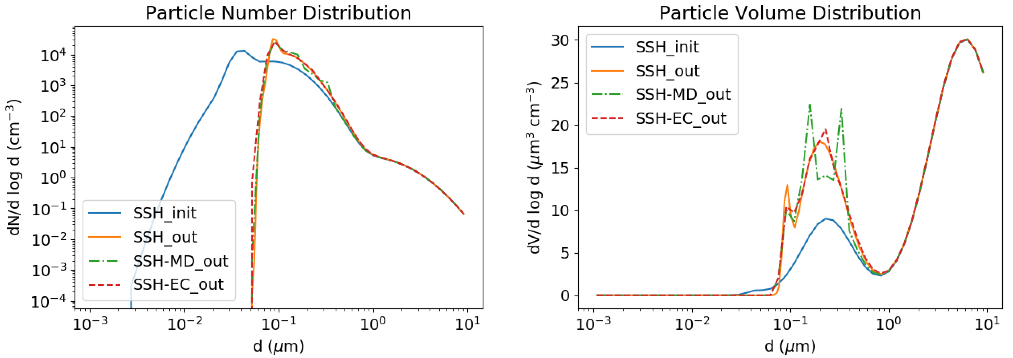
Figure 4.
Condensation/evaporation of inorganic test case. Time evolution of HNO3 concentrations (left) and NH3 concentrations (right).
Figure 4.
Condensation/evaporation of inorganic test case. Time evolution of HNO3 concentrations (left) and NH3 concentrations (right).

Figure 5.
Kelvin test case. Number (left) and volume (right) concentrations. The initial concentrations are in blue, those simulated by SSH-aerosol are in orange (with Kelvin effect) and in dashed green (without Kelvin effect), and those simulated by Devilliers et al. [22] with 48 size sections are displayed with red stars.
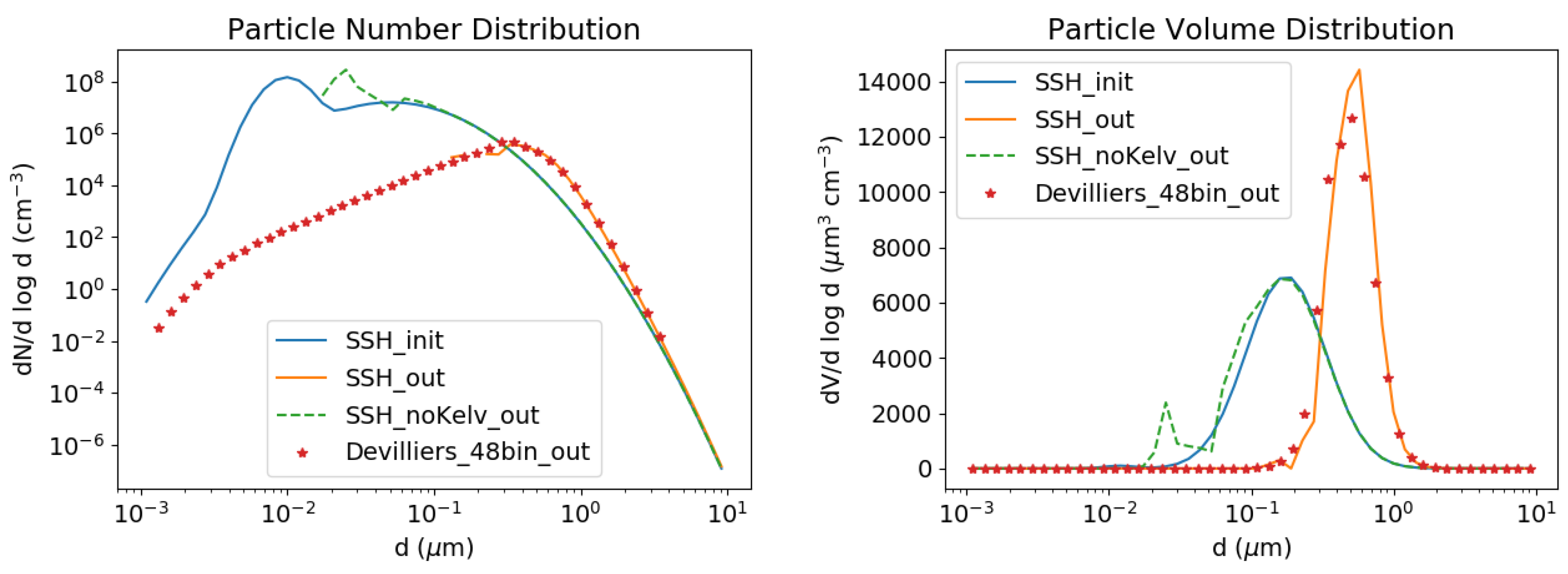
Figure 6.
Viscosity test case: time evolution of organic concentrations ((a) SOAlP; (b) POAlP; and (c) POAmP) for several organic-phase diffusivities: 10−18 (dark blue), 10−19 (light blue), 10−20 (green), 10−21 (yellow), 10−22 (magenta), 10−23 (red) and 10−24 (black) m2 s−1.
Figure 6.
Viscosity test case: time evolution of organic concentrations ((a) SOAlP; (b) POAlP; and (c) POAmP) for several organic-phase diffusivities: 10−18 (dark blue), 10−19 (light blue), 10−20 (green), 10−21 (yellow), 10−22 (magenta), 10−23 (red) and 10−24 (black) m2 s−1.
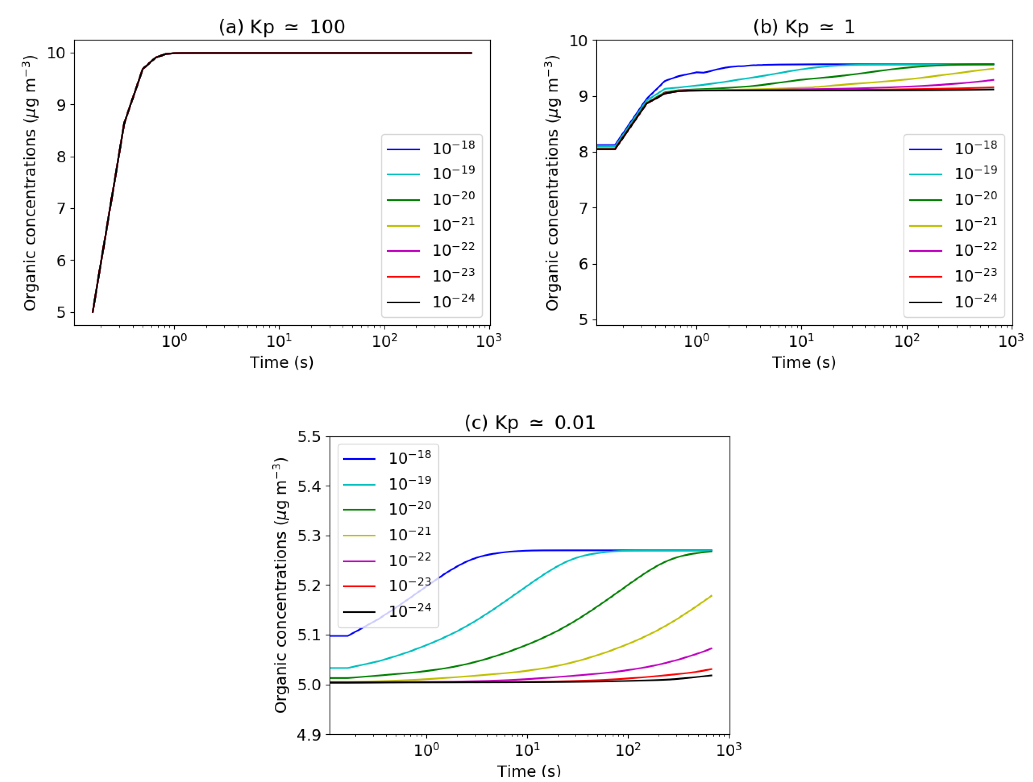
Figure 7.
Particle number concentration (# m−3) for the coagulation test case, as a function of size and composition: initial concentrations (left) and after 12 h of simulation (right).
Figure 7.
Particle number concentration (# m−3) for the coagulation test case, as a function of size and composition: initial concentrations (left) and after 12 h of simulation (right).

Figure 8.
Particle mass concentration (g m−3) for the condensation test case, as a function of size and composition: initial concentrations (left) and after 12 h of simulation (right).
Figure 8.
Particle mass concentration (g m−3) for the condensation test case, as a function of size and composition: initial concentrations (left) and after 12 h of simulation (right).

Figure 9.
Time evolution of organic and inorganic concentrations for the exhaust test case: without NH3 emissions (left) and with NH3 emissions (right).
Figure 9.
Time evolution of organic and inorganic concentrations for the exhaust test case: without NH3 emissions (left) and with NH3 emissions (right).
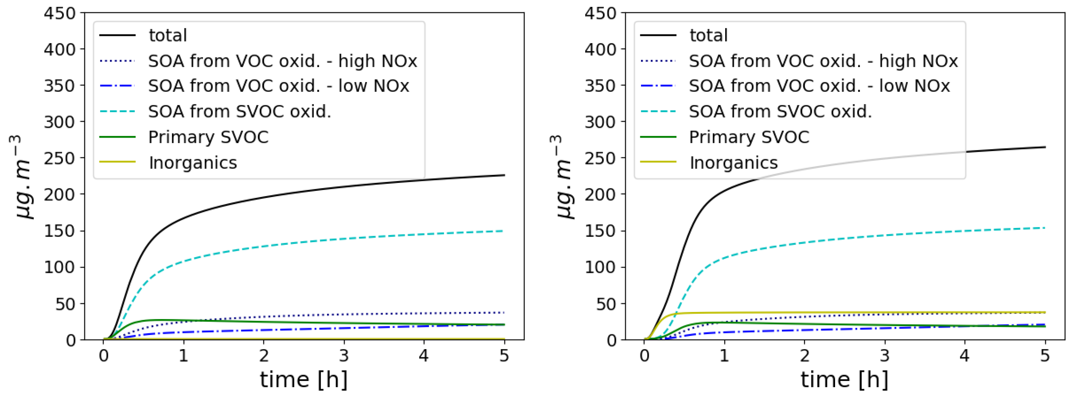
Figure 10.
Time evolution of isoprene SOA in the particle phase.
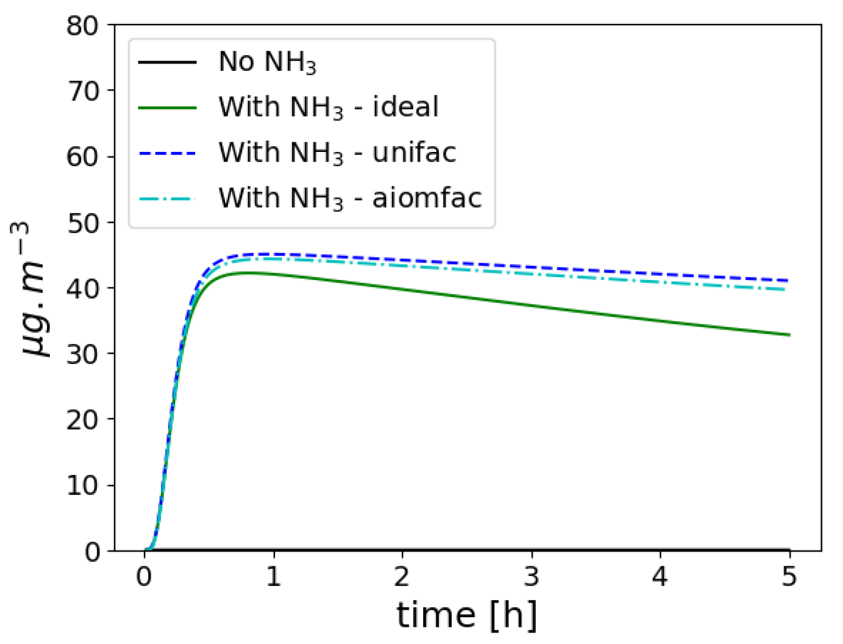
Figure 11.
Nucleation test case. Number (left) and volume (right) concentrations. The initial concentrations are in blue; the simulated concentrations without Monomer are in orange and with Monomer in green. The simulated concentrations with Monomer but solving condensation after coagulation every 60 s are in red.

Figure 12.
Time evolution of the number distribution (# m−3) for the different size sections, without Monomer (left) and with Monomer (right).
Figure 12.
Time evolution of the number distribution (# m−3) for the different size sections, without Monomer (left) and with Monomer (right).

© 2020 by the authors. Licensee MDPI, Basel, Switzerland. This article is an open access article distributed under the terms and conditions of the Creative Commons Attribution (CC BY) license (http://creativecommons.org/licenses/by/4.0/).
Share and Cite
MDPI and ACS Style
Sartelet, K.; Couvidat, F.; Wang, Z.; Flageul, C.; Kim, Y. SSH-Aerosol v1.1: A Modular Box Model to Simulate the Evolution of Primary and Secondary Aerosols. Atmosphere 2020, 11, 525. https://doi.org/10.3390/atmos11050525
AMA Style
Sartelet K, Couvidat F, Wang Z, Flageul C, Kim Y. SSH-Aerosol v1.1: A Modular Box Model to Simulate the Evolution of Primary and Secondary Aerosols. Atmosphere. 2020; 11(5):525. https://doi.org/10.3390/atmos11050525
Chicago/Turabian StyleSartelet, Karine, Florian Couvidat, Zhizhao Wang, Cédric Flageul, and Youngseob Kim. 2020. "SSH-Aerosol v1.1: A Modular Box Model to Simulate the Evolution of Primary and Secondary Aerosols" Atmosphere 11, no. 5: 525. https://doi.org/10.3390/atmos11050525
Note that from the first issue of 2016, this journal uses article numbers instead of page numbers. See further details here.