Satellite-Based Study and Numerical Forecasting of Two Tornado Outbreaks in the Ural Region in June 2017


1
A.M. Obukhov Institute of Atmospheric Physics, Russian Academy of Sciences, 119017 Moscow, Russia
2
Department of Cartography and Geoinformatics, Perm State University, 614990 Perm, Russia
3
Department of Meteorology, Perm State University, 614990 Perm, Russia
*
Author to whom correspondence should be addressed.
Atmosphere 2020, 11(11), 1146; https://doi.org/10.3390/atmos11111146
Submission received: 27 September 2020
/
Revised: 18 October 2020
/
Accepted: 19 October 2020
/
Published: 22 October 2020
(This article belongs to the Special Issue Tornadoes in Europe: Climatology, Forecasting, and Impact)
Abstract
:Strong tornadoes are common for the European part of Russia but happen rather rare east of the Urals. June 2017 became an exceptional month when two tornado outbreaks occurred in the Ural region of Russia, yielded $3 million damage, and resulted in 1 fatality and 14 injuries. In this study, we performed detailed analysis of these outbreaks with different data. Tornadoes and tornado-related environments were diagnosed with news and eyewitness reports, ground-based meteorological observations, sounding data, global numerical weather prediction (NWP) models data, synoptic charts, satellite images, and data of specially conducted aerial imaging. We also estimated the accuracy of short-term forecasting of outbreaks with the WRF-ARW mesoscale atmospheric model, which was run in convection-permitting mode. We determined the formation of 28 tornadoes during the first outbreak (3 June 2017) and 9 tornadoes during the second outbreak (18 June 2017). We estimated their intensity using three different approaches and confirmed that, based on the International Fujita scale (IF), one of the tornadoes had the IF4 intensity, being the first IF4 tornado in Russia in the 21st century and the first-ever IF4 tornado reported beyond the Ural Mountains. The synoptic-scale analysis revealed the similarity of two outbreaks, which both formed near the polar front in the warm part of deepening southern cyclones. Such synoptic conditions yield mostly weak tornadoes in European Russia; however, our analysis indicates that these conditions are likely favorable for strong tornadoes over the Ural region. Meso-scale analysis indicates that the environments were favorable for tornado formation in both cases, and most severe-weather indicators exceeded their critical values. Our analysis demonstrates that for the Ural region, like for other regions of the world, combined use of the global NWP model outputs indicating high values of severe-weather indices and the WRF model forecast outputs explicitly simulating tornadic storm formation could be used to predict the high probability of strong tornado formation. For both analyzed events, the availability of such tornado warning forecast could help local authorities to take early actions on population protection.
1. Introduction
Tornadoes are one of the most devastating and hard-to-predict atmospheric phenomena observed in mid-latitudes. Moreover, the threat of tornadoes in Europe and Russia is substantially underestimated [1,2,3]. In particular, it was considered for a long time that tornadoes occur mainly in European Russia and are extremely rare east of the Urals [4]. Recently, Chernokulsky et al. [2] showed that tornadoes are common for both European and Asian parts of Russia but confirmed that strong tornadoes (≥F3 on the Fujita scale [5]) are substantially less frequent east of the Urals. Particularly, all F4 tornadoes and 92% of all F3 tornadoes for the 979–2016 period occurred in European Russia [2]. Thus, two tornado outbreaks occurred in June 2017 in the Ural region were exceptional events since they included one F3 and, more importantly, one F4 tornado—the first violent tornado east of the Ural Mountains. The outbreaks yielded $3 million damage and resulted in 1 fatality and 14 injuries. Given the impact and rareness of these events, their diagnostics and study of forecasting possibility deserve detailed analysis.
Recently, numerous tornado case-studies in Russia and other European countries have appeared based on observations and reanalyses data [6,7,8,9], satellite and aerial images [10,11,12,13], and data from weather radars [8,9,14]. These studies focused mostly on post-event damage assessment [10,13,15,16], estimates of mesoscale peculiarities of tornado formation and development [9,12,17,18,19], and refinements of regional values of associated severe-weather indicators (so-called ‘ingredients’) [7,9,17,20]. In particular, using satellite data on windthrow areas, Shikhov and Chernokulsky [10] restored actual tornado tracks of the 1984 Ivanovo tornado outbreak in Russia. Rodriguez and Bech [13] used high-resolution aerial images to estimate tornado intensity during the event of 2 November 2008 in Catalonia. Novitskii et al. [20] showed the prognostic power of severe-weather ingredients for the tornado event in the center of European Russia on 23 May 2013.
Mesoscale numerical weather prediction (NWP) models are another powerful tool that are used in studies of tornado environments but also in assessing the possibility of tornado forecasting [17,18,21,22]. Mesoscale NWP models have been used for short-term tornado forecasting from the middle of the 2000s [23,24] when the first successful prediction of tornadic supercell storms was theoretically shown [25,26,27]. Under the NOAA Hazardous Weather Testbed Spring Experiment, the first real-time high-resolution numerical forecasts by the mesoscale Weather Research and Forecasting (WRF) model were provided [24,28]. Afterward, an algorithm for detecting mesocyclones in hourly high-resolution numerical model output was proposed [29] based on the computation of updraft helicity. WRF-based midlevel (2–5 km above ground level, AGL) updraft helicity later were successfully used to localize the tornado path generated by supercell storms [30,31,32]. In [33], low-level (0–1 km AGL) vertical relative vorticity was found more appropriate to identify the tornadic vortices in simulated supercells. Numerous studies have assessed the possibility of short-term tornado forecasting using ingredient-based methodology and analyzed severe-weather indicators simulated by NWP models [11,17,20,34,35]. Studies [36,37,38] have also focused on the sensitivity of the tornado forecasts to cloud and precipitation microphysics parameterization schemes in the WRF model [39], to forecast lead-time [21], and to assimilation of observational data, like data from lightning detection systems [37] or from radars and satellites [38]. The WRF model is widely used to study environments of single tornadoes or tornado outbreaks throughout the world [17,40,41,42,43,44], including Russia [11,14,19,20,45]. It is of note that in most studies, the model reproduced tornado-generating convective storm and even rotating updraft, but the spatial position and timing of the tornado had substantial differences compare to observations. This displacement remains even if the tornado is explicitly simulated by the model [46]. Thus, despite the impressive increase in the computational power and progress in the NWP development, short-term forecasting of tornadoes with sufficient accuracy in space and time remains challenging. It can be especially difficult in regions, where violent tornadoes have not been observed previously.
In the present study, we performed detailed analysis of two tornado outbreaks that occurred in June 2017 in the Asian part of Russia, namely on 3 June 2017 in Sverdlovsk region and on 18 June 2017 in Kurgan and Tyumen regions. Both outbreaks caused substantial economic loss and forest damage that were associated with tornadoes, severe wind gusts, and large hail. The total damage of the 3 June 2017 outbreak amounted to 170 million rubles (~$3,000,000). In addition, one person died and 11 were injured [47]. The 18 June 2017 outbreak caused three injures and substantial damage in the Kurgan and Tyumen regions, especially in Maloye Pesyanovo village, which was partly destroyed [48]. The intensity of the tornado that hit Maloye Pesyanovo village was preliminary estimated as F4 [49], which makes this event the first-ever F4 tornado that has passed beyond the Urals. However, this assessment requires careful verification.
We examined synoptic-scale and mesoscale environments of two tornado outbreaks’ formation using different data, including numerical experiments with the WRF model. We estimated the model performance to forecast the events as well as model sensitivity to grid size and forecast lead time (from 12 to 36 h). Since Doppler radar data were unavailable for the study area, the validation of WRF simulation results was performed with the Meteosat-8 satellite images and satellite-based estimates of tornado-induced disturbances in forests. We describe the experimental design in Section 2. Section 3 presents the results of synoptic-scale and mesoscale analysis of the events and analysis of the tornadoes’ impact, while Section 4 provides the main results of the numerical simulation of tornadic storms. Section 5 summarizes the main findings of the paper.
2. Data and Methods
2.1. Overview of the Data Sources
We used various data sources to obtain the most complete information on the characteristics of the analyzed severe weather outbreaks of 3 and 18 June 2017. These data are summarized below.
Ground-based observations included regular observations from the weather stations of Russian state weather service (69 stations in the Sverdlovsk, Tyumen, and Kurgan regions) and sounding data obtained from the University of Wyoming database [50] that were selected based on the proximity sounding approach [51]. For the event of 3 June 2017, we used the 1200 UTC sounding of Verhnee Dubrovo station (WMO ID: 28445). However, we failed to find suitable sounding data for the event of 18 June 2017.
Severe weather reports included compiled eye-witness photo, video, and damage reports from the media, social networks, and from the European Severe Weather Database [49] and were used to clarify the tornadoes’ impact, path, and intensity.
Satellite data included medium-resolution images from the Landsat-8 and Sentinel-2 satellites and high-resolution images from Google Earth, which were both used to identify forest damage tracks induced by windstorms and tornadoes, and estimate the path length, width, and intensity of the tornadoes (see Section 2.2 for more details). Additionally, we used the Meteosat-8/SEVIRI images, obtained from the EUMETSAT Earth Observation portal [52], to explore convective storms’ evolution, identify the signatures of intense updrafts, and validate the WRF model skills in storm track forecasting. We used the RGB (Red–Green–Blue) combination of the High-Resolution Visible (HRV) and 10.8 μm infrared (IR10.8) spectral bands, known as “HRV cloud”, and also cloud top temperature estimated by the IR10.8 band, to detect overshooting tops (OTs), cold-ring, and cold U/V (CRCUV)-shaped features on the cloud top. According to previous studies [12,53,54,55,56], OTs and CRCUV-shaped signatures indicate strong updrafts and mesocyclones in mesoscale convective systems (MCSs).
In addition, we obtained high-resolution aerial orthophotographs (with 0.2 m pixel size) of the damage track of the tornado that passed near Visim settlement on 3 June 2017. Aerial imagery was performed using a quadcopter on 18 May 2018 along the tornado track. In total, an area of 20 km long and 1 km wide was covered by orthophotographs.
Synoptic-scale fields of atmospheric variables were obtained from the short-term forecast data of the GFS (Global Forecast System [57]) and GEM (Global Environmental Multiscale Model [58]) NWP models. Synoptic charts obtained from the Roshydromet archive were also utilized. The GFS and GEM models forecasts (with ~25 km grid size) from 0000 UTC 03 June 2017 and 0000 UTC 18 June 2017 were downloaded from the NCEP [57] and CMC [58] ftp-servers, respectively.
Thermodynamic and kinematic parameters (diagnostic variables or so-called ‘ingredients’), related to tornadogenesis, were calculated using GFS and GEM model outputs. We calculated the following severe-weather indicators: surface-based (SB) convective available potential energy (CAPE), SB convective inhibition (CIN), SB lifted index (LI), 0–3 km storm relative helicity (SRH), low-level (0–1 km) wind shear (LLS), deep layer (0–6 km) wind shear (DLS), and composite parameters, such as WMAXSHEAR [59], energy-helicity index (EHI) [60], supercell composite parameter (SCP) [60], and significant tornado parameter (STP) [3] (see Table A1 for details). The SB CAPE and SB CIN parameters came as output models, while the other parameters were computed. Calculations were performed within the Open GrADS package.
The WRF mesoscale NWP model with the ARW (Advanced Research WRF) dynamic core version 3.8.1 (WRF-ARW) [39] was used for explicit simulation of MCSs (see Section 2.3 for details).
2.2. Tornado Tracks Identification and Characteristics Estimate
Initial data on the studied tornado events was obtained from eye-witness observations and damage reports, presented in news and social media and then further uploaded to the European Severe Weather Database [49] by one of the authors (IA) of this study. However, the intensity of tornadoes was estimated preliminarily, while the characteristics of the tornado paths were mostly undetermined. We examined them in this paper using various satellite observations. In particular, we used satellite data in three-stage searching of tornado damage tracks in forests of storm-affected regions.
For the first stage, we used pre- and post-event Landsat-8 and Sentinel-2 images downloaded from the USGS Data Archive [61]. We applied the previously proposed method of tornado track identification in forested regions [10,62,63] and delineated numerous windthrow areas caused by tornadoes and storm winds. Additionally, we used the Global Forest Change data [64] to confirm the identified forest loss areas.
For the second stage, we analyzed high-resolution satellite images available on Google Earth to confirm or reject potential tornadic nature of windthrow areas, based on its typical signatures [13,62,63]. Most of the storm-affected region was covered by summertime high-resolution images in 2017–2018 (after the storm events), which allowed to determine the cause of windthrow, i.e., discriminate between a tornado and squall. Using high-resolution images, we visually inspected in detail areas adjacent to storm- and tornado-damage tracks identified by Sentinel-2 images and found several additional tornado tracks. Some of them partially overlapped with squall-induced windthrow areas.
For the third stage, we used the Meteosat-8/SEVIRI images to improve the searching of tornado tracks, which could be missed after the first and second stage. We searched OTs and CRCUV-shaped features on the cloud tops, which indicate intense updrafts [12,53,54,55,56], and delineated their tracks. Along these tracks, we performed additional visual inspection of local windthrow areas using high-resolution images from Google Earth. This procedure helped us to discover several previously unknown tornado tracks.
We used high-resolution images to determine tornado/squall path geometrical characteristics. In the absence of high-resolution images, we used the Sentinel-2 data. We determined the path length, maximum width, and damaged area. More details on the procedure of geometrical characteristics determination can be found in [62,63].
For tornado events, we estimated tornado intensity along with geometrical characteristics. Most of the tornadoes passed outside of settlements and were found only with the use of satellite images of forest damage tracks. Ideally, forest damage survey or high-resolution aerial imagery of damaged forest is needed to correctly estimate the intensity of such tornadoes [13,15,65,66]. Due to their lack, we used high-resolution (with ~0.5 m pixel size) satellite images from Google Earth to assess tornado intensity. The spatial resolution of satellite images is several times lower than the same of aerial images; however, they can provide valuable information to estimate tornado damage. In particular, we used three different approaches.
The first approach of tornado intensity estimation is based on the recommendations for the International Fujita (IF) Scale [65], which were elaborated by the European Severe Storm laboratory, and can be applied to Russian forest species and, with some assumptions, to Russian buildings. It was primarily applied for tornadoes covered by photo or video damage reports. With substantial limitations, this method may be applied to tornadoes identified using high-resolution satellite images of damaged forests. Particularly, we examined the forest damage degree that may be of partial or total canopy removal (less and more than 75% of windthrow area), which corresponds to the IF0 and ≥IF1 tornado intensity, respectively [65]. It is important to note that all widespread tree species in tornado-damaged forests (spruce, pine, birch, and aspen) are classified as low firmness species (softwood) according to [65]. Therefore, tornado having intensity ≥IF1 is able to destroy forest stands. However, we did not able to determine whether the trees were uprooted, snapped, or debarked because of the tornado, which can indicate higher intensity levels [65]. The one exception is the tornado that passed near Visim and was covered by high-resolution aerial images. We found this the tornado caused total canopy removal and snapped most coniferous trees within the damage track, while deciduous trees were mostly felled down; as a result, we rated it as IF2 [65].
The second method of the enhanced Fujita (EF) scale intensity determination is based on the approach proposed by Peterson et al. [66]. Within this approach, the EF-scale level is a function of forest damage severity, which is expressed as the percentage of uprooted or snapped trees on 100 × 100 m areas. For instance, the EF0 level corresponds to 18–38% of areas of blown trees (10–48% within the 95% confidence interval) (see Figure 7 from [66] for details). We applied this approach for tornadoes that damaged forest stands and for which we had post-event high-resolution satellite images. Note, we did not estimate the EF-rating based on recommendations [67] since they were proposed for U.S. construction practices. The approach [66] should also be used with caution since it was developed using linkages between forest wind resistance and wind speed that were obtained for forest species in North America rather than northern Eurasia.
The third approach allows to determine minimum probable Fujita-scale intensity based on tornado path length and width [2,10,62]. We used Weibull distribution parameters from [68] that link tornado intensity with path length and maximum width. The approach is described in full in [62] (see particularly their Figure 6). It was applied for all tornadoes whose path characteristics were determined.
Combining three approaches, we assigned the most probable intensity rating (on the IF-scale) to all tornadoes that occurred on 3 June and 18 June 2017 that were restored using the aforementioned approaches. The Appendix presents the list of these tornadoes (Table A2) and also the list of strong wind events reported at weather stations and based on forest damage analysis (Table A3).
2.3. WRF Model Configuration and Forecast Accuracy Assessment
We used the WRF-ARW v.3.8.1 model to simulate the analyzed events. This is a non-hydrostatic model with several parameterization options [39,69]. We performed several numerical experiments with different horizontal grid spacing, with and without a nested grid. We used the GFS-NCEP model forecast with a 0.25° grid size as initial and boundary conditions. The model was run in a convection-permitting mode, which was previously found to be optimal for tornadic storm simulation [29,33,41,42,45,46]. We used explicit convection-permitting simulation since most of the simulated convective storms were meso-α-scale events. The nudging procedure was not implemented. Table 1 summarizes the WRF model settings, and Figure 1 shows the model domains.
The sensitivity numerical experiments with the WRF-ARW model included two main steps. On the first step, we estimated the influence of horizontal resolution on the results of tornadic storm simulation. The simulation was performed with the horizontal grid spacing of 9, 7.2, and 3 km. For the 9-km grid spacing, one nested domain with a 3-km resolution grid performed with the one-way nesting technique was included. The model assimilated the GFS-NCEP data for 0000 UTC of 3rd and 18th June 2017 for the first and second events and operated for 24 h till 0000 UTC of 4th and 18th June 2017, respectively. Since both tornadoes were observed around 1200 UTC, we could consider this experiment as a forecast with an approximately 12-h lead time. As a result, we determined the most appropriate model configuration (in terms of resolution) to simulate tornadic storms with this lead time (see Section 4 for more details).
On the second step, we estimated the sensitivity of forecast accuracy to the lead time. The WRF model assimilated the GFS-NCEP data for 0000 and 1200 UTC of preceding days, i.e., 2 June 2017 and 17 June 2017, respectively. As a result, we obtained the forecasts of tornadic storms with 24- and 36-h lead times. For this experiment, we used the model configuration that provided a more accurate forecast on the first step.
The Doppler radar system installed in Russia does not cover the region of interest yet [70]. Therefore, we used the Meteosat-8 SEVIRI satellite images to validate results of the WRF outputs. We compared satellite-observed and WRF-simulated characteristics of convective tornadic storms—path, timing, and cloud top temperature. Additionally, the location and timing of simulated storms was compared with the observed tornado tracks.
Tornadic storms were identified based on sea-level pressure (SLP), 0–3 km SRH, maximum radar reflectivity, and 10 m wind speed fields. In particular, we considered that meso-scale low pressure systems (having 4–10 hPa depth), high values of SRH (>1000 m2 s−2), and strong wind gusts (≥30 m s−1) with well-pronounced wind convergence indicated potential tornadic storms. Similar approaches used to identify convective storms based on WRF model outputs have been successfully used previously (see, e.g., [17,42,45]). We should stress that the use of SRH alone may not have meaningful application since simulated convective cells themselves significantly affect wind field and SRH. In theory, the updraft helicity may better indicate rotating updrafts (i.e., supercell mesocyclone) (see, e.g., [22,32,33]); however, due to some technical issues, we did not calculate this parameter in our analysis.
3. Storm Events Description
In May and June 2017, a deep and unusually long-lived tropospheric trough dominated over the European Russia and caused a long-term period of cold and wet weather with average temperature below the norm by 2–4 °C. Arctic cold air masses spread to the Black, Caspian, and Aral Seas, inducing the formation of several southern cyclones that moved to the Ural region. These cyclones yielded favorable conditions for convective storm development, specifically on 3 June 2017 and 18 June 2017. These days, severe weather outbreaks with heavy rainfalls, strong wind ≥25 m s−1, large hail up to 40 mm, and tornadoes formed in the Sverdlovsk and Kurgan/Tyumen regions, respectively. Both events caused substantial damage to settlements, agricultural crops, and forests. One fatality and at least 14 injuries were reported.
3.1. Large-Scale Synoptic Features
On 3 June 2017, the Ural region was influenced by the forward side of a deep tropospheric cyclone with a center over north of European Russia. The frontal zone stretched over the Ural Mountains from south to north with a temperature gradient up to 12 °C/500 km at 850 hPa between rather cold European Russia (−5 °C) and warm Western Siberia (up to 18 °C). A mid-tropospheric jet stream with wind speeds up to 35 m s−1 at 500 hPa stretched from the southern part of European Russia to Western Ural.
In the afternoon of 2 June 2017, a surface low (with SLP ~1000 hPa) formed on the polar front between Caspian and Aral Seas. After 0000 UTC 3 June, it began to move with speed around 16–22 m s−1 along the jet stream. At 1200 UTC 3 June, the low deepened (SLP amounted to 993 hPa) and centered near 55° N, 60° E, where it resulted in a severe weather outbreak (Figure 2a). Afterward, the low moved northward to the Northern Ural and continued to deepen (up to 987 hPa at 0000 UTC 4 June 2017).
In the afternoon of 3 June 2017, the polar front stretched along the Ural Mountains. It divided cold air mass to the west (i.e., in the Perm region), with the maximum air temperature at 2 m AGL (Tmax) around +16°…+20 °C, and warm air mass to the east (i.e., in the Sverdlovsk and Chelyabinsk regions) with Tmax up to +31 °C. Severe convective storms with squalls, large hail, and tornadoes formed in the warm sector and on the cold front near the occlusion point. The synoptic situation of the 3 June 2017 event generally corresponds to the second typical scheme of tornado formation over Northern Eurasia according to [4].
On 18 June 2017, the eastern part of the Ural region was influenced by a forward side of a tropospheric low centered over the Volga region. A waving polar front stretched from south to north over northern Kazakhstan and the Kurgan and Tyumen regions. The frontal zone in the middle troposphere was similarly oriented; wind speed at 500 hPa did not exceed 25 m s−1.
A low with SLP ~1000 hPa formed in the afternoon of 17 June on the polar front over the Central Kazakhstan. After 2000 UTC, it began to abruptly deepen and moved northward, with speeds up to 19 m s−1 along the jet stream in the middle troposphere. At 1200 UTC 18 June, the low centered approximately at 56° N, 67° E with 992 hPa SLP (Figure 2b). In the next hours, its movement direction changed to northwestern and speed decreased to 8–11 m s−1. At 0600 UTC 19 June, the low centered over the western part of the Tyumen region, and SLP decreased to 982 hPa.
Deep convection started near the occlusion point of the cyclone at 0930 UTC 18 June when the temperature gradient over the polar front was up to 12–14 °C/500 km at 850 hPa. As for the first event, the synoptic situation of this event corresponds to the second typical scheme of tornado formation over Northern Eurasia according to [4].
3.2. Diagnostic Variables, Estimated by the Global NWP Models, and Sounding Data
Several thermodynamic and kinematic variables (indices) related to the formation of tornadoes were calculated according to the GFS/NCEP and GEM/CMC data. We used the so-called proximity soundings approach [60] and found the maximum values of the severe-weather indices estimated within a 100-km area around the observed tornadoes. The selected indices are most frequently used to estimate the risk of tornadogenesis (see, e.g., [17,22,40,41,42,43,44,59]).
According to the NWP-based calculating indices, on 3 June 2017 between 0900 and 1500 UTC, the environments were favorable for the development of severe thunderstorms and tornadoes in the Sverdlovsk and Chelyabinsk regions (Table 2, Figure 3). In particular, most of indices exceeded critical values. That is, CAPE ranged from 1500 to 2000 J kg−1 and low-level shear (LLS) reached 15 m s−1 according to the GEM data. These high values of LLS indicate the presence of a low-level jet stream that could contribute to the formation of tornadoes. Simultaneously, DLS was rather low for tornado occurrence (4 and 8 m s−1 according to the GFS and GEM, respectively). However, it is very likely that both NWP models substantially underestimated it, since DLS was 20 m s−1 according to the sounding data. Models showed the highest values of 0–3 km SRH (up to 480 m2 s−2) near the axis of the trough oriented along the Ural Mountains. The maximum calculated EHI values exceeded 2.0 (up to 4.2 according to GFC), which is considered favorable for tornado occurrence [42]; STP values were also above the critical level (1.0); however, the SCP parameter lacked predictive power for this event (Table 2).
The GFC-based soundings are sensitive to grid point selection. In particular, the sounding in the actual tornado point (Figure 3a) showed unusually high lifted condensation level. In fact, such conditions with dry air mass spreading from south-east in the low-layer were observed 100 km east of the tornado-affected area. It is of note that such environments resulted in dry squalls (severe wind gusts with almost no precipitation) in the central and southeastern parts of the Sverdlovsk region. The sounding data from the Verhnee Dubrovo station obtained at 1200 UTC 3 June 2017 confirmed the presence of low-layer dry air (CAPE was only 11 J kg−1) and indicated relatively high wind shear, with mid-tropospheric (at 511 hPa) wind speeds reaching 27 m s−1, and a well-pronounced low-level, jet stream with wind speed reaching 18.5 m s−1 at the 879 hPa level. LLS and DLS amounted to 14 and 20 m s−1, respectively. Therefore, the sounding data actually were more representative for observed dry squalls than for tornadoes.
For the event of 18 June 2017, extremely high convective instability (CAPE ≥ 3000 J kg−1) was observed over the eastern part of the Kurgan region between 0900 and 1500 UTC (Table 2). LLS and DLS reached 11 and 21 m s−1, respectively. The hodograph (Figure 3) displayed a pronounced ‘kink’ near the 900 hPa surface, where a combination of weak directional shear and strong speed shear abruptly changed to strong directional shear, which was likely associated with a low-level mesocyclone [76]. Other parameters were also above their critical levels. SRH exceeded 450 m2 s−2, the maximum value of EHI reached 5.0, SCP and STP amounted to 3.5 and 2.9, respectively, while CIN amounted to −72 J kg−1. Thus, the atmospheric environments were exceptionally favorable for the development of a severe weather outbreak, including strong tornadoes.
3.3. Convective Storms Evolution
The evolution of convective storms was analyzed using the Meteosat-8 images with the 15-min time resolution. Weather station data and eye-witness reports were also utilized.
On 3 June 2017, a deep convection started already at 0400 UTC on the south of the Chelyabinsk region. In the next few hours, the MCS, which developed near the occlusion point of the cyclone, increased its size up to 250 km and moved northward; severe wind gusts (up to 27 m s−1, see Table A3 for details) and large hail (with a diameter up to 35 mm, Table A3) were reported at the weather stations in the Chelyabinsk region.
At 0830 UTC, an isolated convective cell with cloud top temperature (CTT) of −60 °C formed over northeastern Bashkortostan, behind the front. According to eye-witness observations, the cell contained a mesocyclone. At 1115 UTC, a well-pronounced OT with CTT −62 °C was observed by the Meteosat-8 image near Staroutkinsk (the western part of the Sverdlovsk region), where the first IF2 tornado of that day was reported (Figure 4a,b). Next 30 min, OT transformed to the cold-ring feature with a diameter of 80 km (Figure 4c,d). At the same time, the second significant tornado passed near Visim. After 1200 UTC, the storm weakened. Another isolated storm, which probably contained a mesocyclone, formed at 0945 UTC, 100 km to the north of the track of the first storm. It passed between 1100 and 1200 UTC near Biser weather station (WMO ID 28138), where a large hail (32 mm) was reported.
Afterward, between 1130 and 1330 UTC, another convective storm formed on the cold front and moved through the Chelyabinsk region and the western part of the Sverdlovsk region. It caused widespread damaging winds (22–27 m s−1) and numerous mostly weak tornadoes (IF0–IF1, one IF2), which were identified by the high-resolution satellite images. It is of note that severe wind gusts caused more substantial damage than tornadoes. After 1330 UTC, the MCS merged with two isolated storms and formed mesoscale convective complex (MCC) with a major axis diameter of about 400 km, and CTT decreased down to −65 °C. The MCC further yielded several weak (IF0–IF1) tornadoes and one IF2-tornado, severe wind gusts, and large hail in the north of the Sverdlovsk region and northeast of the Perm region (Table A2 and Table A3). It reached a maximum intensity near Kachkanar, where 400 ha of forest were totally damaged by a windstorm.
On 18 June 2017, deep convection started at 0900 UTC near the occlusion point of a cyclone (see Section 3.1). At 0945 UTC, several separate convective cells merged to MCC, the size of which increased rather explosively, and CTT decreased below −60 °C. About 11.00 UTC, two tornadoes were reported in the eastern part of the Kurgan region, near Tsentralnoye and Kravtsevo villages. The strongest tornado destroyed Maloye Pesyanovo village around 1145 UTC. The mesocyclone, which generated this strong tornado, is well-detected on the Meteosat-8 image, where OT with extremely low CTT (−65 °C) and cold-ring signatures were also observed on the cloud top (Figure 5). At 1300 UTC, the MCC moved from the Kurgan region to the Tyumen region; its diameter exceeded 400 km. Strong wind gusts (24–26 m s−1) and heavy rainfalls were reported at weather stations, and four relatively weak tornadoes formed in the Tyumen and Sverdlovsk regions. The MCC weakened and dissipated after 2000 UTC.
3.4. The Main Characteristics of Tornadoes and Associated Severe Weather Events
We found 28 tornadoes for the 3 June 2017 event and 9 tornadoes for the 18 June 2017 event (Figure 6, Table A2) by collecting and analyzing eye-witness observations and damage reports in the media, as well as evaluating forest damage using satellite data. Among all tornadoes, 29 cases were found with high-resolution satellite images only, while 8 tornadoes were reported by eye-witnesses. Information on seven tornadoes was confirmed by two or more independent data sources. We estimated the certainty of events (see [2] for details of this procedure) and defined the high level of certainty for 32 tornadoes, and the medium level for five tornadoes.
Among 28 tornadoes of 3 June 2017, the strongest tornado passed near Visim and damaged forest on the area of 4.97 km2 (Figure 7b,c). Its intensity substantially depends on the method of estimating (Table A2). In particular, according to the method [66], the intensity is estimated as EF4, since more than 80% of trees were blown down or snapped in 100 m × 100 m forest areas. However, tree debarking (which is considered a signature of ≥IF3 intensity) cannot be confirmed by aerial images; additionally, it is important to note that spruce and birch trees were mostly uprooted than snapped. Therefore, based on the recommendations for the International Fujita Scale [65], the tornado intensity should be estimated at the IF2 level, taking into account the domination of low-firmness trees in the analyzed region. On the contrary, geometrical characteristics of the tornado path, i.e., the length of 33.3 km (the longest tornado path for both outbreaks) and the maximum width of 1590 m (the second widest) put the tornado intensity to the at least F3 category with a 90% probability (Table A2). Considering the three estimates and mismatch between F-/IF- and EF-scales, we speculate that this tornado likely has IF3 intensity.
Another significant tornado that day passed through Staroutkinsk, where it seriously damaged dozens of houses and damaged forest in the area of 1.57 km2 (Figure 7a). Other tornadoes passed through forested area and caused local windthrows (mostly corresponding to the IF0 or IF1 intensity levels). The total area of stand-replacing windthrow caused by the severe weather outbreak of 3 June 2017 was estimated as 15.4 km2.
Most of the tornadoes of 18 June 2017 passed mainly over a treeless area (Figure 6) and were reported by eye-witnesses. The strongest tornado hit Maloye Pesyanovo village at 1135 UTC and blew down four strong log-houses; also, tree debarking was reported (Figure 8c). According to the recommendations for the International Fujita scale [65], the near complete destruction of log houses can be considered as an indicator of IF4 damage since the sturdiness of such houses is somewhat equal to sturdiness of ‘strong framehouses’ (Thilo Kühne, personal communication). The violent character of this tornado is also supported by two other intensity estimates. Particularly, the tornado has the EF5 intensity level according to the method [66] (up to 100% of trees were blown down or snapped in 100 m × 100 m forest areas). Given tornado path length (20.3 km) and maximum width (1750 m, the widest for both outbreaks), the minimal tornado intensity was estimated as F3 with 90% probability. Consequently, our estimates confirm the formation of the first IF4 tornado in Russia in the 21st century (after the previous one in 1984 [10]) and the first-ever IF4 tornado reported beyond the Urals.
4. Results of Modeling
In this section, we present the results of cloud-resolving simulation of tornadic thunderstorms using the WRF-ARW mesoscale model [39]. To estimate the forecast accuracy, we compared the simulated severe storms, i.e., their paths and intensity as well as cloud top characteristics, with the observed tornado tracks and the Meteosat-8 images. In Section 4.1, we describe the results of the performed experiments with various model grid spacings and with the 12-h lead time. Section 4.2 contains an assessment of the model performance with one selected grid spacing but with various (24- and 36-h) lead times.
4.1. WRF Model Forecasts with Various Horizontal Grid Spacing
4.1.1. Determination of the Most Appropriate Model Grid Spacing
We performed three simulations for both tornado events, with model settings described in Section 2.3 with a 12-h lead time (model start from 0000 UTC 3 June 2017 and 0000 UTC 18 June 2017). To assess the forecast reliability, firstly we determined the presence of potentially tornadic storms in the model output (see Section 2.3 for details). Then, if a storm was predicted by the model, we estimated the location and timing errors by comparing the simulated storm location with that observed on the Meteosat-8 images, and simulated the tornadic storm track with the Landsat-based tornado tracks. Figure 9 and Figure 10 and Table 3 present the results of simulation with the use of three various model grid spacings for 1200 UTC 3 June 2017 and 1300 UTC 18 June 2017, respectively.
The tornadic storm of 3 June 2017 was reproduced by the model only with the version with the 3-km grid spacing and no nested grid (Figure 9a). An isolated storm (a meso-scale low) with SRH up to 1075 m2 s−2 and composite reflectivity ~58 dBz was predicted between 1200 and 1400 UTC, reaching the maximum intensity at 1300 UTC according to the model output. However, the simulated intensity of the severe storm was underestimated since wind gusts did not exceed 17 m s−1. The timing error of the forecast was about 1–1.5 h.
The WRF model configuration with a 7.2-km grid resolution did not predict isolated storms that could generate tornadoes (Figure 9b). The simulation with a 9-km grid resolution and a 3-km nested grid (Figure 9c) predicted two storms with high composite reflectivity (>50 dBz) that moved east of the observed tornado track and had no above-mentioned storm signatures. We failed to simulate strong wind gusts (>20 m s−1) with any WRF model settings. In general, we can conclude that none of the three simulations performed at 00 UTC 3 June 2017 allowed prediction of the tornadoes that occurred on 3 June 2017.
The 18 June 2017 tornadic storm over the Kurgan region was simulated by the WRF model accurately, in particular with the version with the 3-km grid spacing and no nested grid (Figure 10a). At 1300 UTC, the model predicted well-pronounced meso-scale low severe convective storm with composite reflectivity up to 64 dBz, severe wind gust up to 31 m s−1, and SRH ~1200 m2 s−2. The simulated severe storm track and observed tornado track had a displacement less than 10 km. Considering that the model with the 3-km resolution does not allow simulation of the tornado itself, this forecast can be estimated as successful.
However, the simulated severe storm passed near Maloye Pesyanovo village around 1300 UTC, whereas the actual tornado occurred at 1135 UTC (Table A2). This time lag (1 h 25 min) is presumably associated with the GFS model assimilated data, since the lag time is independent of the WRF model configuration.
The forecasts of tornadic storm of 18 June 2017 with other WRF model settings (Figure 10 b,c) were less accurate. The model predicted a severe storm track 30 km to the east of the observed tornado track. However, this storm was not confirmed neither by the Meteosat-8 images nor the forest damage analysis. Instead of a tornadic storm, the model predicted a squall line, which in addition was slightly shifted to the west compared to the tornado track.
For both cases, the 10–30-km displacement between the simulated storm tracks and observed tornado tracks is generally in line with results obtained previously [22,42,77]. Our findings on the simulation of two or more tornadic storms instead of one observed storm (as in the case of 18 June 2017) is in agreement with [22,45].
Comparing three WRF model configurations for both events, we found the most appropriate accuracy of tornadic storm forecast using the WRF model configuration with the 3-km grid spacing and no nested grid. Further, we considered this model configuration as optimal for a short-term forecast of severe storms for the analyzed events.
4.1.2. Validation of the Simulation Results with the Meteosat-8 Images
The MCSs characteristics (CTT and composite reflectivity) simulated with all three WRF model configurations were overlapped with the Meteosat-8 images. Table 4 presents the simulated and satellite-derived CTTs, as well as location and timing errors that were estimated by comparing simulated and observed spatial position of convective storms. Figure 11 and Figure 12 present the convective storms at the time of tornado occurrence based on the Meteosat-8 images and the WRF simulations with the optimal model configuration (3-km resolution, no nested grid).
For the first case (3 June 2017, Figure 11), one can see that the WRF-simulated and satellite-observed location and geometry of the northern severe storm match rather well. Simulated and observed CTT values range from −55 to −60 °C. It is of note that the cold-ring signature on the cloud top is also well-reproduced by the model. Nevertheless, the forecast cannot be considered as successful, since the model entirely missed the main MCS that formed on the cold front 100 km to the south of the first storm and caused wind-related damage.
For the second case (18 June 2017, Figure 12), the tornado-generating MCC with a diameter exceeding 400 km was well-predicted by the model. Several well-detected OTs and cold-ring signatures are seen on the cloud top. It is important to note that the OTs correspond to the zones with simulated high composite reflectivity. One OT moved along the tornado track with only a 10-km displacement. The main shortcoming of the simulation is the substantial time error. Indeed, despite the simulated and observed MCC tracks having similarity, the simulated MCC moved with a 1.5-h lag compare to the satellite-based one (Table 4).
4.2. Sensitivity of Simulation Results to Forecast Lead Time
The WRF model with a 3-km resolution and no nested grid started at 0000/1200 UTC 2 June 2017 and 17 June 2017 and was used to estimate the influence of the forecast lead time on the accuracy of simulation. Table 5 summarizes the obtained results, and Table 6 presents the comparison of simulated MCSs characteristics with the Meteosat-8 data.
The model predicted the convective storms with high composite reflectivity and strong wind gusts independently of the forecast lead time. The most reliable forecast of the event of 3 June 2017 was obtained from 1200 UTC 2 June 2017 (i.e., with the 24-h lead time) when the model predicted a storm with a well-pronounced meso-scale low-pressure system, very high SRH (up to 1350 m2 s−2), and wind gusts up to 28 m s−1 (Figure 13b). The forecast with the 36-h lead time is also relatively successful, since the model predicted the convective storm but shifted 50 km to the east (Figure 13b). Both forecasts (24 and 36 h) have a substantial timing error (1.25–1.5 h). In particular, at 1200 UTC, the simulated storm was 20 km to the south of the start of the first tornado track. In fact, at this time, the tornado had already passed near Visim town, 70 km to the north of its simulated location.
In the second case (18 June 2017), the model predicted the convective storm with strong wind gusts (up to 30 m s−1) but with relatively low values of SRH (≤600 m2 s−2). Thus, the forecast of the 18 June 2017 storm with the 24- and 36-h lead time in principal can be used to warn severe wind gusts but not tornadoes. The forecast time error was approximately the same as for the 12-h lead time forecast.
5. Discussion and Conclusions
In this study, we evaluated the environments of the formation of two tornado outbreaks that occurred east of the Ural Mountains on 3 June and 18 June 2017 using different data. For tornado diagnostics, we used news reports, eyewitness reports, ground-based meteorological observations, sounding data, global NWP models data, synoptic charts, satellite data on forest disturbances, and data of the specially conducted aerial imaging. We also estimated the accuracy of short-term forecasting of outbreaks with the WRF-ARW atmospheric model.
Both analyzed outbreaks caused substantial damage associated with tornadoes, severe wind gusts, and large hail. We found the 3 June 2017 outbreak is rather rare in terms of the number of tornadoes—we confirmed the formation of 28 tornadoes. Four of them were significant (≥IF2 intensity), including one strong tornado (IF3). Convective storms moved mainly over forest-covered area, which made it possible to identify tornado damage tracks in forests using the Sentinel-2 data, high-resolution satellite images, and data of the aerial imaging performed for the strongest tornado of this outbreak. The characteristics of tornado paths were determined, i.e., tornado width and length. On the contrary, the outbreak 18 June 2017 occurred over mainly treeless area. Therefore, it is probably that the number of tornadoes within this outbreak is underestimated, since they cannot be found with satellite data. In addition, the geometric characteristics of tornado paths were determined not for all tornadoes. The outbreak includes four significant tornadoes, including one violent tornado that hit Maloye Pesyanovo village—the first IF4 tornado in Russia in the 21st century and the first-ever IF4 tornado recorded beyond the Ural Mountains.
Only four tornadoes that passed through settlements and one tornado that was covered by aerial imaging have solid estimates of tornado intensity. The intensity of other tornadoes was determined rather approximately. We used three different methods to estimate their intensity based on satellite data only. We used the recommendations for International Fujita scale [65], which allowed us to discriminate tornadoes with IF0 intensity among all others. Using satellite data, we failed to reveal the signatures of trees’ damage indicating higher tornado intensity; particularly, it was impossible to see whether trees were snapped or debarked. We also used our method developed in [10,62], which is based on the relationship between Fujita-scale tornado intensity and tornado path width and length [68]. This method provides only a minimal intensity rating (i.e., ≥F2) and cannot be used when there is a lack of data on tornado track characteristics. In addition, the tornado intensity estimate may be incorrect for short-lived tornadoes. The third used approach is based on the method of Godfrey and Peterson [66], who tied EF-scale tornado intensity with forest damage severity. We found this method generally overestimated the intensity of the analyzed tornadoes. It is of note that the method had been developed using linkages between forest wind resistance and wind speed obtained for North American forest species [66]. Presumably, this linkage is not well suited for northern Eurasian forests. This issue deserves further research.
The analysis of synoptic-scale environments revealed the similarity of the two outbreaks. Both events formed in the afternoon hours (at local time), when the development of a deep convection reached a daily maximum [2]. Additionally, both events formed near the cold polar front in the warm part of deepening southern cyclones, close to their occlusion points. Tropical air masses spread from Kazakhstan, and the high precipitable water content (up to 42 mm on 18 June 2017 and 30 mm on 3 June 2017) was related mainly to strong convergence near the cyclone center and local evaporation from the well-moistened underlying surface. Such synoptic-scale environments are favorable for tornado occurrence both in the Ural region [11,16] and in the European part of Russia [6,14,16,19]. The synoptic situations of both events correspond to the second typical scheme of tornado formation over northern Eurasia according to Snitkovsky [4]. Based on the statistics for the European part of Russia, Snitkovsky had found that this type yields mostly weak tornadoes [4]. However, events analyzed in the study resulted in IF3 and IF4 tornadoes, which indicates the need to reconsider Snitkvosky schemes for other Russian regions (i.e., the Ural, Siberia, Far East). This can be achieved using data from the new climatology presented in [2].
The characteristics of tornado-generating MCSs were substantially different in the first and second cases. On 3 June 2017, two significant tornadoes were induced by the long-lived severe storm that was formed in the warm sector. Additionally, numerous weak tornadoes occurred when there was a mesoscale convective system on the cold front. On 18 June 2017, tornadoes were associated with mesocyclones embedded into a rapidly increasing mesoscale convective complex that formed on the cold front. In both cases, a well-pronounced OT and cold-ring signatures on the cloud top coincided in space and time with tornado occurrence.
Short-term forecast based on the global NWP models (GFS and GEM) produced critical values of diagnostic variables (severe-weather indices) that indicate tornado formation for both events. In particular, a rare combination of strong convective instability (CAPE > 1500 J/kg) and low-level wind shear (>10 m s−1) was found. Such environments are favorable for tornado occurrence in the U.S. [21,51] and in Europe [17,59]. An exceptionally high value of EHI (up to 4.0 and 5.0 for the first and second events) and STP (2.5 and 2.9) also unambiguously pointed to a high risk of formation of strong tornadoes.
The specially conducted short-term forecasts with the convection-permitting WRF model were rather successful in both cases. The model reproduced the formation of severe convective storms, which somewhat coincides in space and time with the observed tornado tracks. However, for the 3 June event, the model failed to reproduce the main storm (the second storm of that day), which induced widespread severe wind. For the 18 June event, the model reproduced the formation of the MCC with several well-pronounced meso-scale lows and wind gusts > 30 m s−1. In both cases, the WRF model configuration with the 3-km grid spacing and no nested grid provided the most reliable forecast. We also evaluated the forecast sensitivity to the lead time (12–36 h) and found that the model simulated the convective storms somewhat independently of the forecast lead time. We should stress that it is necessary to evaluate more cases of tornadoes and tornado outbreaks to determine the optimal configuration of the WRF model and estimate the sensitivity of simulated storm tracks characteristics (e.g., their location and timing errors) to a forecast lead time.
Operational short-term tornado forecasting is not implemented in Russia. Our analysis demonstrates that combined use of the global NWP model outputs indicating high values of severe-weather indices and the WRF model forecast outputs explicitly indicating convective storms and meso-cyclones formation could be used to predict the high probability of strong tornado occurrence. For both analyzed events, such tornado warning forecast could help local authorities to take early action on population protection. However, it should be highlighted that the frequency of false alarms in WRF-based short-term forecasts of tornadic storms remains unexplored, at least for the territory of northern Eurasia. To obtain such estimates, one needs to build and analyze long-term series of mesoscale NWP models output data, e.g., The Spring Experiment conducted in the USA [24,28]. In the future, we are planning to set-up and analyze such experiments for several Russian regions.
Supplementary Materials
The following are available online at https://www.mdpi.com/2073-4433/11/11/1146/s1, Contain animation of satellite data for HRV cloud RGB images and IR10.8 channel data (cloud top temperature) for both events. In addition, the location of tornadoes and their most probable IF-intensity rating is shown. File names are 20170603_CTT.mp4 and 20170618_CTT.mp4 for IR10.8 animations; 20170603_HRVcloud.mp4 and 20170618_HRVcloud.mp4 for HRV cloud RGB animations.
Author Contributions
Conceptualization, methodology, writing and visualization—A.C. and A.S.; initial data collection and tornado intensity estimate— I.A. and A.C.; synoptic-scale and mesoscale analysis—A.S. and A.B.; numerical experiments with WRF model—A.B.; validation—A.S. All authors have read and agreed to the published version of the manuscript.
Funding
The study was funded by the Ministry of Science and Higher Education of the Russian Federation under the agreement No 075-15-2020-776.
Conflicts of Interest
The authors declare no conflict of interest.
Appendix A. Information on Severe Weather Indices Calculations and Additional Information on Tornadoes and Squalls

Table A1.
Diagnostic variables calculated from the GFS and GEM data.
| Indices (Acronym) | Indices (Full Name) | Equation | Reference |
|---|---|---|---|
| SB CAPE, J Kg−1 | Surface-based convective available potential energy | [78] | |
| SB CIN, J Kg−1 | Surface-based Convective inhibition | [78] | |
| SB LI, °C | Surface-based Lifted Index | [78] | |
| LLS, m s−1 | Low-level shear | [59] | |
| DLS, m s−1 | Deep layer shear | [59] | |
| WMAXSHEAR, m2 s−2 | WMAXSHEAR | [59] | |
| 0–3 km SRH, m2 s−2 | 0–3 km Storm-Relative Helicity | [78] | |
| EHI | Energy-helicity Index | [60,78] | |
| SCP | Supercell Composite Parameter | [60] | |
| STP | Significant Tornado Parameter | [3] |
The following notations are used: LFC—height of level of free convection, EL—height of equilibrium level, Tv,parcel—virtual temperature of the individual parcel (lifted from surface), Tv,env—virtual temperature of the environment, T’500—virtual temperature at 500 hPa, T’p,500—virtual temperature of lifted parcel at 500 hPa, V—wind speed, k—vertical unit vector, C—moving velocity of cell, Vh—wind vector, MUCAPE—most unstable CAPE, SBLCL—Surface-based Lifted Condensation Level. Subscripts denote vertical levels (surf—near surface; 900 and 500—corresponding isobaric levels; 0–3—the layer from surface to 3 km height; 0–1—the layer from the surface to 1 km height).
Table A2.
List of tornado events that occurred on 3 June 2017 and 18 June 2017.
| Tornado Number | Data Quality | Coordi Nates (Start) | Coordi- Nates (End) | Time (UTC) | Data Sources | The Most Probable Intensity Rating and Three Tornado Intensity According to Various Methods * | Damaged Settlements | Damage to Settlements and Infrastructure | Move- Ment Direction | Forest Damage Track | |
|---|---|---|---|---|---|---|---|---|---|---|---|
| Path Length (km) and Maximum Width (m) | Confirmation with High-Resolution Image and Its Date | ||||||||||
| 3 June 2017 | |||||||||||
| 1.1 | Medium | 56.231 N 59.743 E | 56.234 N 59.737 E | 1055 | Satellite data | IF0 IF0/-/≥F0 | 4 km SW of Kenchurka | Forest damage | SE-NW | 0.5/100 | - |
| 1.2 | High | 57.190 N 59.310 E | 57.429 N 59.410 E | 1115 | Eyewitness photo and video, damage photo and video, satellite data | IF2 IF2/EF4/≥F2 | Staroutkinsk | Dozens of houses damaged, roofs destroyed, forest damage (total canopy removal) | SSW- NNE | 28.5/1240 | + 12 May 2019 |
| 1.3 | High | 57.482 N 59.414 E | 57.769 N 59.462 E | 1145 | Eyewitness video, damage photo, satellite and aerial images | IF3 IF2/EF4/≥F3 | 4 km from Visim | Forest damage (total canopy removal) | SSW- NNE | 33.3/1590 | + 5 Oct 2019 7 Oct 2019 |
| 1.4 | High | 57.338 N 59.747 E | 57.354 N 59.757 E | 1215 | Satellite data | IF1 ≥IF1/EF0/≥F1 | 9 km WNW of Polovinny | Forest damage | SSW-NNE | 1.9/240 | + 14 Sep 2017 |
| 1.5 | Medium | 59.264 N 59.120 E | 59.268 N 59.116 E | 1215 | Satellite data | IF0 -/-/F0 | 27 km SSW of Kytlym | Forest damage | SSE-NNW | 0.6/100 | - |
| 1.6 | High | - | - | 1220 | Eyewitness video | IF0 -/-/- | Near Beloyarsky | No damage | - | -/- | - |
| 1.7 | High | 56.816 N 61.376 E | 56.829 N 61.383 E | 1225 | Satellite data | IF1 ≥IF1/EF1/≥F1 | 3 km ENE of Zarechny | Forest damage | SSW- NNE | 1.5/140 | + 12 May 2019 |
| 1.8 | High | 57.278 N 60.590 E | 57.284 N 60.589 E | 1245 | Satellite data | IF1 ≥IF1/EF1/≥F0 | 5 km NW of Ol’khovka | Forest damage | SSE- NNW | 0.7/100 | + 29 Aug 2017 |
| 1.9 | High | 57.770 N 60.396 E | 57.773 N 60.394 E | 1250 | Satellite data | IF1 ≥IF1/EF1/≥F0 | 3 km E of Vilyui | Forest damage | SSE- NNW | 0.3/70 | + 18 Jul 2017 |
| 1.10 | High | 57.774 N 60.233 E | 57.817 N 60.242 E | 1250 | Satellite data | IF2 ≥IF1/EF1/≥F2 | 4 km E of Shilovka | Forest damage | S-N | 4.8/490 | + 11 Aug 2017 |
| 1.11 | High | 57.694 N 59.975 E | 57.724 N 59.974 E | 1250 | Satellite data | IF1 ≥IF1/EF2/≥F1 | 6 km ESE of Chernoistochnik | Forest damage | S-N | 3.4/210 | + 30 Jun 2018 |
| 1.12 | High | 57.870 N 60.222 E | 57.893 N 60.220 E | 1255 | Satellite data | IF1 ≥IF1/EF1/≥F1 | 6 km E of Zonal’ny | Forest damage | S-N | 2.6/310 | + 11 Aug 2017 |
| 1.13 | High | 57.936 N 60.220 E | 57.942 N 60.219 E | 1300 | Satellite data | IF1 IF0/EF0/≥F1 | 4 km SW of Pokrovskoe | Forest damage | SSE- NNW | 0.7/150 | + 11 Aug 2017 |
| 1.14 | High | 58.011 N 60.306 E | 58.042 N 60.319 E | 1315 | Satellite data | IF1 ≥IF1/EF2/≥F1 | 1 km NNE of Molodezhny | Forest damage | SSW- NNE | 3.5/280 | + 2 Sep 2017 |
| 1.15 | High | 58.078 N 60.267 E | 58.085 N 60.273 E | 1315 | Satellite data | IF1 ≥IF1/EF0/≥F0 | 8 km NW of Svobodny | Forest damage | SSW- NNE | 0.8/80 | + 2 Sep 2017 |
| 1.16 | High | 58.127 N 60.399 E | 58.138 N 60.395 E | 1315 | Satellite data | IF1 ≥IF1/EF1/≥F1 | 10 km N of Svobodny | Forest damage | SSE- NNW | 1.3/200 | + 23 May 2018 |
| 1.17 | High | 58.670 N 60.177 E | 58.688 N 60.173 E | 1400 | Satellite data | IF1 ≥IF1/EF2/≥F1 | 4 km E of Novaya Tura | Forest damage | SSE- NNW | 2.1/280 | + 19 Jul 2019 |
| 1.18 | High | 58.959 N 59.763 E | 58.984 N 59.752 E | 1415 | Satellite data | IF1 ≥IF1/EF1/≥F1 | 2 km W of Chernichny | Forest damage | SSE- NNW | 3.0/360 | + 7 Sep 2019 |
| 1.19 | Medium | 60.564 N 58.994 E | 60.583 N 59.012 E | 1430 | Satellite data | IF1 -/-/≥F1 | 27 km E of Ust-Uls | Forest damage | SSW- NNE | 2.4/140 | - |
| 1.20 | High | 59.167 N 61.386 E | 59.186 N 61.370 E | 1445 | Satellite data | IF1 ≥IF1/EF1/≥F1 | 3 km WNW of Yakimovo | Forest damage | SSE- NNW | 2.3/170 | + 14 Sep 2019 |
| 1.21 | Medium | 59.493 N 61.156 E | 59.496 N 61.148 E | 1530 | Satellite data | IF0 -/-/F0 | 12 km NNW of Krasnoglinny | Forest damage | SE-NW | 0.6/60 | - |
| 1.22 | Medium | 59.800 N 61.019 E | 59.850 N 60.948 E | 15:30 | Satellite data | IF1 -/-/F1 | 13 km E of Krasny Yar | Forest damage | SE-NW | 6.8/300 | - |
| 1.23 | High | 59.800 N 60.520 E | 59.816 N 60.501 E | 1540 | Satellite data | IF1 ≥IF1/EF3/≥F1 | 3 km NNE of Podgarnichny | Forest damage | SE-NW | 2.2/200 | + 3 Sep 2018 |
| 1.24 | High | 59.967 N 59.849 E | 59.977 N 59.860 E | 1545 | Satellite data | IF1 ≥IF1/EF1/≥F0 | 5 km NNE of Sosnovka | Forest damage | SSW- NNE | 1.4/90 | + 7 Aug 2017 |
| 1.25 | High | 59.935 N 60.528 E | 59.975 N 60.487 E | 1545 | Satellite data | IF2 ≥IF1/EF1/≥F2 | 4 km NW of Lar’kovka | Forest damage | SSE- NNW | 5.1/510 | + 7 Aug 201723 Aug 2017 |
| 1.26 | High | 60.259 N 59.924 E | 60.272 N 59.920 E | 1600 | Satellite data | IF1 ≥IF1/EF1/≥F1 | 5 km NW of Kal’ya | Forest damage | SSE- NNW | 1.6/270 | + 5 Jul 2017 |
| 1.27 | High | 60.661 N 59.407 E | 60.681 N 59.398 E | 1610 | Satellite data | IF1 IF0/EF0/≥F1 | 34 km ESE of Vels | Forest damage | SSE- NNW | 2.5/130 | + 11 Aug 2017 |
| 1.28 | High | 60.661 N 59.504 E | 60.690 N 59.503 E | 1630 | Satellite data | IF1 IF0/EF0/≥F1 | 30 km NW of Vsevolodo-Blagodatskoe | Forest damage | S-N | 3.3/220 | + 11 Aug 2017 |
| 18 June 2017 | |||||||||||
| 2.1 | High | 55.145 N 66.590 E | 55.238 N 66.585 E | 1105 | Eyewitness video, satellite data | IF2 ≥IF1/EF4/≥F2 | Baksary | Forest damage (total canopy removal) | S-N | 10.5/900 | + 1 Mar 2018 |
| 2.2 | High | - | - | 1105 | Eyewitness video | IF0 -/-/- | NE of Baksary | No damage | - | - | - |
| 2.3 | Medium | - | - | 1110 | Eyewitness report | IF0 IF0/-/- | Tsentralnoe | Few roofs of houses slightly damaged | - | - | - |
| 2.4 | High | 55.501 N 66.636 E | 55.670 N 66.560 E | 1135 | Eyewitness report, damage photo and video, satellite data | IF4 IF4/EF5/≥F3 | Maloye Pes’yanovo | Four houses totally destroyed, another 25 seriously damaged, forest damage (total canopy removal) | SSE- NNW | 20.3/1750 | + 30 Jun 2017 |
| 2.5 | High | 55.668 N 66.458 E | 55.752 N 66.420 E | 1145 | damage photo, satellite data | IF2 IF2/EF3/≥F2 | Novotroitskoe | Houses damaged, forest damage (total canopy removal) | SSE- NNW | 10.0/790 | + 30 Jun 2017 |
| 2.6 | High | 56.452 N 66.493 E | 56.496 N 66.437 E | 1300 | Eyewitness video, satellite data | IF2 ≥IF1/EF4/≥F2 | 4 km WSW of Zavodoukovsk | Forest damage (total canopy removal) | SE-NW | 6.0/580 | + 27 Apr 2018 |
| 2.7 | High | 57.133 N 65.303 E | 57.153 N 65.275 E | 1350 | Satellite data | IF1 ≥IF1/EF3/≥F1 | 2 km E of Gor’kovka | Forest damage | SE-NW | 2.9/280 | + 24 Aug 2017 |
| 2.8 | High | 57.269 N 66.417 E | 57.273 N 66.407 E | 1400 | Satellite data | IF1 ≥IF1/EF2/≥F1 | 13 km E of Kunchur | Forest damage | SE-NW | 0.7/200 | + 2 Aug 2017 |
| 2.9 | High | 58.061 N 64.415 E | 58.074 N 64.383 E | 1545 | Satellite data | IF1 ≥IF1/EF1/≥F1 | 6 km NNW of Saragulka | Forest damage | SE-NW | 2.4/190 | + 14 Jul 2018 |
Table A3.
List of strong squall events (reported at the weather stations or caused forest damage) occurred on 3 June 2017 and 18 June 2017.
Table A3.
List of strong squall events (reported at the weather stations or caused forest damage) occurred on 3 June 2017 and 18 June 2017.
| Report Type | Coordinates (Weather Station or Central Point of Windthrow Area) | WMO ID of the Weather Station | Time (UTC) | Reported Wind Gust (m s−1) | Damaged Settlements | Damage Description | Accompanied Weather Events | Move- Ment Direction | Forest Damage Track | |
|---|---|---|---|---|---|---|---|---|---|---|
| Path Length (km) and Maximum Width (km) | Damaged Area, ha | |||||||||
| 3 June 2017 | ||||||||||
| Weather station report | 57.88 N 60.07 E | 28440 | 1300 | 26 | Nizhniy Tagil | One fatality, 10 injured, 166 million rubles (~$3 millions) of damage (buildings, cars and trees damaged) | Heavy rainfall | S-N | - | - |
| 54.55 N 60.30 E | 28741 | 25 | Mirniy | Trees and cars damaged, power supply of 46 settlements was interrupted | Hail with 35 mm in daimeter | S-N | - | - | ||
| 57.45 N 61.17 E | 28345 | 1200 (±1 h) | 27 | Lipovskoe | No data | No data | S-N | - | - | |
| Forest damage | 58.71 N 60.16 E | - | 1400 (±1 h) | - | - | Trees damaged in Lesnoy and Nizhnya Tura | No data | S-N | 6.7/1.3 | 50 |
| 58.12 N 60.07 E | - | 1300 | - | - | Buildings, cars and trees damaged in Nizhniy Tagil | No data | S-N | 31.0/22.2 | 192 | |
| 58.81 N 59.51 E | - | 1400 (±1 h) | - | - | Buildings, cars and trees damaged in the nearest towns Kachkanar | Hail with 40 mm in daimeter | S-N | 24.8/3.1 | 472 | |
| 18 June 2017 | ||||||||||
| Weather station report | 56.02 N 65.70 E | 28561 | 1200 (±1 h) | 26 | Pamyatnoe | Power lines damage, tree damage | No data | SSE- NNW | - | - |
| 55.28 N 66.50 E | 28662 | 1100 (±1 h) | 25 | Lebyazhie | Power lines damage, tree damage | No data | SSE- NNW | - | - | |
| Forest damage | 55.71 N 66.48 E | - | 1200 (±30 min) | - | - | Buildings and trees damaged in the settlements of the Mokrousovsky district | No data | SSE- NNW | 19.1/5.1 | 37 |
References
- Antonescu, B.; Schultz, D.M.; Holzer, A.; Groenemeijer, P. Tornadoes in Europe: An Underestimated Threat. Bull. Am. Meteorol. Soc. 2017, 98, 713–728. [Google Scholar] [CrossRef]
- Chernokulsky, A.; Kurgansky, M.; Mokhov, I.; Shikhov, A.; Azhigov, I.; Selezneva, E.; Zakharchenko, D.; Antonescu, B.; Kühne, T. Tornadoes in Northern Eurasia: From the Middle Age to the Information Era. Mon. Weather Rev. 2020, 148, 3081–3111. [Google Scholar] [CrossRef] [Green Version]
- Grieser, J.; Haines, P. Tornado Risk Climatology in Europe. Atmosphere 2020, 11, 768. [Google Scholar] [CrossRef]
- Snitkovskiy, A.I. Tornadoes in the USSR. Sov. Meteorol. Gidrol. 1987, 9, 12–25. (In Russian) [Google Scholar]
- Fujita, T.T. Tornadoes and downbursts in the context of generalized planetary scales. J. Atmos. Sci. 1981, 38, 1511–1534. [Google Scholar] [CrossRef] [Green Version]
- Finch, J.; Bikos, D. Russian tornado outbreak of 9 June 1984. Electron. J. Sev. Storms Meteorol. 2012, 7, 1–28. [Google Scholar]
- Kurgansky, M.V.; Chernokulsky, A.V.; Mokhov, I.I. The tornado over Khanty-Mansiysk: An exception or a symptom? Russ. Meteorol. Hydrol. 2013, 38, 539–546. [Google Scholar] [CrossRef]
- Hannesen, R.; Dotzek, N.; Gysi, H.; Beheng, K.D. Case study of a tornado in the Upper Rhine valley. Meteorol. Z. 1998, 7, 163–170. [Google Scholar] [CrossRef]
- Wesolek, E.; Mahieu, P. The F4 tornado of August 3, 2008, in Northern France: Case study of a tornadic storm in a low CAPE environment. Atmos. Res. 2011, 100, 649–656. [Google Scholar] [CrossRef]
- Chernokulsky, A.V.; Shikhov, A.N. 1984 Ivanovo tornado outbreak: Determination of actual tornado tracks with satellite data. Atmos. Res. 2018, 207, 111–121. [Google Scholar] [CrossRef]
- Shikhov, A.N.; Bykov, A.V. Study of two cases of severe tornadoes in the Predural’e region. Sovrem. Probl. Distantsionnogo Zondirovaniya Zemli iz Kosm. 2015, 12, 124–133. (In Russian) [Google Scholar]
- Putsay, M.; Simon, A.; Szenyán, I.; Kerkmann, J.; Horváth, G. Case study of the 20 May 2008 tornadic storm in Hungary—Remote sensing features and NWP simulation. Atmos. Res. 2011, 100, 657–679. [Google Scholar] [CrossRef]
- Rodriguez, O.; Bech, J. Reanalysing strong-convective wind damage paths using high-resolution aerial images. Nat. Hazards 2020, 104, 1021–1038. [Google Scholar] [CrossRef]
- Novitskii, M.A.; Pavlyukov, Y.B.; Shmerlin, B.Y.; Makhnorylova, S.V.; Serebryannik, N.I.; Petrichenko, S.A.; Tereb, L.A.; Kalmykova, O.V. The tornado in Bashkortostan: The potential of analyzing and forecasting tornado-risk conditions. Russ. Meteorol. Hydrol. 2016, 41, 683–690. [Google Scholar] [CrossRef]
- Rodríguez, O.; Bech, J.; Soriano, J.D.D.; Gutiérrez, D.; Castán, S. A methodology to conduct wind damage field surveys for high-impact weather events of convective origin. Nat. Hazards Earth Syst. Sci. 2020, 20, 1513–1531. [Google Scholar] [CrossRef]
- Chernokulsky, A.V.; Kurgansky, M.V.; Zakharchenko, D.I.; Mokhov, I.I. Genesis Environments and Characteristics of the Severe Tornado in the South Ural on August 29, 2014. Russ. Meteorol. Hydrol. 2015, 40, 794–799. [Google Scholar] [CrossRef]
- Taszarek, M.; Czernecki, B.; Walczakiewicz, S.; Mazur, A.; Kolendowicz, L. An isolated tornadic supercell of 14 July 2012 in Poland—A prediction technique within the use of coarse-grid WRF simulation. Atmos. Res. 2016, 178–179, 367–379. [Google Scholar] [CrossRef]
- Šinger, M.; Púčik, T. A challenging tornado forecast in Slovakia. Atmosphere 2020, 11, 821. [Google Scholar] [CrossRef]
- Dmitrieva, T.G.; Peskov, B.E. Synoptic conditions, nowcasting, and numerical prediction of severe squalls and tornados in Bashkortostan on June 1, 2007 and August 29, 2014. Russ. Meteorol. Hydrol. 2016, 41, 673–682. [Google Scholar] [CrossRef]
- Novitskii, M.A.; Shmerlin, B.Y.; Petrichenko, S.A.; Tereb, L.A.; Kulizhnikova, L.K.; Kalmykova, O.V. Using the indices of convective instability and meteorological parameters for analyzing the tornado-risk conditions in Obninsk on May 23, 2013. Russ. Meteorol. Hydrol. 2015, 40, 79–84. [Google Scholar] [CrossRef]
- Shafer, C.M.; Mercer, A.E.; Doswell, C.A., III; Richman, M.B.; Leslie, L.M. Evaluation of WRF forecasts of tornadic and nontornadic outbreaks when initialized with synoptic-scale input. Mon. Weather Rev. 2009, 137, 1250–1271. [Google Scholar] [CrossRef] [Green Version]
- Pilguj, N.; Taszarek, M.; Pajurek, L.; Kryza, M. High-resolution simulation of an isolated tornadic supercell in Poland on 20 June 2016. Atmos. Res. 2019, 218, 145–159. [Google Scholar] [CrossRef]
- Roebber, P.J.; Schultz, D.M.; Romero, R. Synoptic regulation of the 3 May 1999 tornado outbreak. Weather Forecast. 2002, 17, 399–429. [Google Scholar] [CrossRef] [Green Version]
- Kain, J.S.; Weiss, S.J.; LevIt, J.J.; Baldwin, M.E.; Bright, D.R. Examination of convection-allowing configurations of the WRF model for the prediction of severe convective weather: The SPC/NSSL Spring Program 2004. Weather Forecast. 2006, 21, 167–181. [Google Scholar] [CrossRef] [Green Version]
- Grell, G.; Dudhia, J.; Stauffer, D. A Description of the Fifth-Generation Penn State/NCAR Mesoscale Model (MM5); NCAR Tech. Note NCAR/TN-398 + STR; University Corporation for Atmospheric Research: Boulder, CO, USA, 1996; 117p. [Google Scholar] [CrossRef]
- Xue, M.; Droegemeier, K.K.; Wong, V. The Advanced Regional Prediction System (ARPS)—A multi-scale nonhydrostatic atmospheric simulation and prediction model. Part I: Model dynamics and verification. Meteorol. Atmos. Phys. 2000, 75, 161–193. [Google Scholar] [CrossRef]
- Xue, M.; Wand, D.; Gao, J.; Brewster, K.; Droegemeier, K.K. The Advanced Regional Prediction System (ARPS), storm-scale numerical weather prediction and data assimilation. Meteorol. Atmos. Phys. 2003, 82, 139–170. [Google Scholar] [CrossRef]
- Kain, J.S.; Weiss, S.J.; Bright, D.R.; Baldwin, M.E.; Levit, J.J.; Carbin, G.W.; Schwartz, C.S.; Weisman, M.L.; Droegemeier, K.K.; Weber, D.B.; et al. Some practical considerations regarding horizontal resolution in the first generation of operational convection-allowing NWP. Weather Forecast. 2008, 23, 931–952. [Google Scholar] [CrossRef]
- Weisman, M.L.; Davis, C.; Wang, W.; Manning, K.W.; Klemp, J.B. Experiences with 0–36-h explicit convective forecasts with the WRF-ARW model. Weather Forecast. 2008, 23, 407–437. [Google Scholar] [CrossRef]
- Sobash, R.A.; Kain, J.S.; Bright, D.R.; Dean, A.R.; Coniglio, M.C.; Weiss, S.J. Probabilistic forecast guidance for severe thunderstorms based on the identification of extreme phenomena in convection-allowing model forecasts. Weather Forecast. 2011, 26, 714–728. [Google Scholar] [CrossRef]
- Clark, A.J.; Kain, J.S.; Marsh, P.T.; Correia, J.; Xue, M.; Kong, F. Forecasting tornado pathlengths using a three-dimensional object identification algorithm applied to convection-allowing forecasts. Weather Forecast. 2012, 27, 1090–1113. [Google Scholar] [CrossRef]
- Clark, A.J.; Gao, J.; Marsh, P.T.; Smith, T.; Kain, J.S.; Correia, J., Jr.; Xue, M.; Kong, F. Tornado pathlength forecasts from 2010 to 2011 using ensemble updraft helicity. Weather Forecast. 2013, 28, 387–407. [Google Scholar] [CrossRef] [Green Version]
- Sobash, R.A.; Romine, G.S.; Schwartz, G.S. Explicit Forecasts of Low-Level Rotation from Convection-Allowing Models for Next-Day Tornado Prediction. Weather Forecast. 2016, 31, 1591–1614. [Google Scholar] [CrossRef]
- Púcik, T.; Groenemeijer, P.; Rýva, D.; Kolář, M. Proximity soundings of severe and nonsevere thunderstorms in central Europe. Mon. Weather Rev. 2015, 143, 4805–4821. [Google Scholar] [CrossRef]
- Kalmykova, O.V.; Shershakov, V.M.; Novitskii, M.A.; Shmerlin, B.Y. Automated Forecasting of Waterspouts off the Black Sea Coast of Russia and Its Performance Assessment. Russ. Meteorol. Hydrol. 2019, 44, 764–771. [Google Scholar] [CrossRef]
- Stratman, D.R.; Brewster, K.A. Sensitivities of 1-km forecasts of 24 May 2011 tornadic supercells to microphysics parameterizations. Mon. Weather Rev. 2017, 145, 2697–2721. [Google Scholar] [CrossRef]
- Fierro, A.O.; Mansell, E.R.; Ziegler, C.L.; MacGorman, D.R. Application of a lightning data assimilation technique in the WRF-ARW model at cloud-resolving scales for the tornado outbreak of 24 May 2011. Mon. Weather Rev. 2012, 140, 2609–2627. [Google Scholar] [CrossRef]
- Jones, T.A.; Stensrud, D.; Wicker, L.; Minnis, P.; Palikonda, R. Simultaneous radar and satellite data storm-scale assimilation using an ensemble kalman filter approach for 24 may 2011. Mon. Weather Rev. 2015, 143, 165–194. [Google Scholar] [CrossRef]
- Skamarock, W.; Klemp, J.; Dudhia, J.; Gill, D.; Barker, D. A Description of the Advanced Research WRF Version 3; NCAR Tech., Note NCAR/TN-475+STR; University Corporation for Atmospheric Research: Boulder, CO, USA, 2008. [Google Scholar]
- Litta, A.J.; Mohanty, U.C.; Bhan, S.C. Numerical simulation of a tornado over Ludhiana (India) using WRF-NMM model. Meteorol. Appl. 2010, 17, 64–75. [Google Scholar] [CrossRef]
- Litta, A.J.; Mohanty, U.C.; Prasad, S.K.; Mohapatra, M.; Tyagi, A.; Sahu, S.C. Simulation of tornado over Orissa (India) on March 31, 2009, using WRF–NMM model. Nat. Hazards 2012, 61, 1219–1242. [Google Scholar] [CrossRef]
- Das, M.K.; Das, S.; Chowdhury, M.A.M.; Karmakar, S. Simulation of tornado over Brahmanbaria on 22 March 2013 using Doppler weather radar and WRF model. Geomat. Nat. Hazards Risk 2016, 7, 1577–1599. [Google Scholar] [CrossRef] [Green Version]
- Matsangouras, I.T.; Pytharoulis, I.; Nastos, P.T. Numerical modeling and analysis of the effect of complex Greek topography on tornadogenesis. Nat. Hazards Earth Syst. Sci. 2014, 14, 1905–1919. [Google Scholar] [CrossRef] [Green Version]
- León-Cruz, J.F.; Carbajal, N.; Pineda-Martínez, L.F. Meteorological analysis of the tornado in Ciudad Acuña, Coahuila State, Mexico, on May 25, 2015. Nat. Hazards 2017, 89, 423–439. [Google Scholar] [CrossRef]
- Romanskii, S.O.; Verbitskaya, E.M.; Ageeva, S.V.; Istomin, D.P. Tornado in the City of Blagoveshchensk on July 31, 2011. Russ. Meteorol. Hydrol. 2018, 43, 574–580. [Google Scholar] [CrossRef]
- Schenkman, A.D.; Xue, M.; Hu, M. Tornadogenesis in a high-resolution simulation of the 8 May 2003 Oklahoma City supercell. J. Atmos. Sci. 2014, 71, 130–154. [Google Scholar] [CrossRef]
- Hurricane Damage in Sverdlovsk Region Exceeded 170 Million Rubles. Available online: https://tass.ru/v-strane/4315705 (accessed on 15 September 2018). (In Russian).
- The Hurricane Caused Millions of Damage to the Zauralye Region. Available online: https://www.znak.com/2017-06-21/uragan_nanes_zauralyu_millionnyy_ucherb_kokorin_prerval_otpusk_chtoby_ocenit_obstanovku (accessed on 15 September 2020). (In Russian).
- European Severe Weather Database. Available online: http://www.eswd.eu (accessed on 15 September 2020).
- Sounding Data Archive. Available online: http://weather.uwyo.edu/upperair/np.html (accessed on 15 September 2020).
- Rasmussen, E.N.; Blanchard, D.O. A baseline climatology of sounding-derived supercell and tornado forecast parameters. Weather Forecast. 1998, 13, 1148–1164. [Google Scholar] [CrossRef] [Green Version]
- EUMETSAT Earth Observation Portal. Available online: https://eoportal.eumetsat.int/userMgmt/login.faces (accessed on 15 September 2020).
- Kerkmann, J.; Lutz, H.J.; König, M.; Prieto, J.; Pylkko, P.; Roesli, H.P.; Rosenfeld, D.; Zwatz-Meise, V.; Schmetz, J.; Schipper, J.; et al. MSG Channels, Interpretation Guide, Weather, Surface Conditions and Atmospheric Constituents. 2006. Available online: http://oiswww.eumetsat.org/WEBOPS/msg_interpretation/index.html. (accessed on 15 August 2018).
- Adler, R.F.; Markus, M.J.; Fenn, D.D. Detection of severe midwest thunderstorms using geosynchronous satellite data. Am. Meteorol. Soc. 1985, 113, 769–781. [Google Scholar] [CrossRef] [Green Version]
- Bedka, K.M. Overshooting cloud top detections using MSG SEVIRI Infrared brightness temperatures and their relationship to severe weather over Europe. Atmos. Res. 2011, 99, 175–189. [Google Scholar] [CrossRef]
- Setvák, M.; Lindsey, D.T.; Novák, P.; Wang, P. Satellite-observed cold-ring-shaped features atop deep convective clouds. Atmos. Res. 2010, 97, 80–96. [Google Scholar] [CrossRef]
- GFS Model Operational Forecast Data. Available online: http://nomads.ncep.noaa.gov/pub/data/nccf/com/gfs/prod/ (accessed on 15 September 2020).
- GEM Model Global Operational Forecast Data. Available online: http://dd.weatheroffice.gc.ca/model_gem_global/25km/grib2/lat_lon/ (accessed on 15 September 2020).
- Taszarek, M.; Brooks, H.E.; Czernecki, B. Sounding-derived parameters associated with convective hazards in Europe. Mon. Weather Rev. 2017, 145, 1511–1528. [Google Scholar] [CrossRef]
- Thompson, R.L.; Edwards, R.; Hart, J.A.; Elmore, K.L.; Markowski, P. Close proximity soundings within supercell environments obtained from the Rapid Update Cycle. Weather Forecast. 2003, 18, 1243–1261. [Google Scholar] [CrossRef] [Green Version]
- USGS Earth Explorer. Available online: https://earthexplorer.usgs.gov (accessed on 28 August 2018).
- Shikhov, A.N.; Chernokulsky, A.V. A satellite-derived climatology of unreported tornadoes in forested regions of northeast Europe. Remote Sens. Environ. 2018, 204, 553–567. [Google Scholar] [CrossRef]
- Shikhov, A.N.; Chernokulsky, A.V.; Azhigov, I.O.; Semakina, A.V. A satellite-derived database for stand-replacing windthrows in boreal forests of the European Russia in 1986–2017. Earth Syst. Sci Data Discuss 2020. in review. [Google Scholar] [CrossRef]
- Hansen, M.C.; Potapov, P.V.; Moore, R.; Hancher, M.; Turubanova, S.A.; Tyukavina, A.; Thau, D.; Stehman, S.V.; Goetz, S.J.; Loveland, T.R.; et al. High-Resolution Global Maps of 21st-Century Forest Cover Change. Science 2013, 342, 850–853. [Google Scholar] [CrossRef] [PubMed] [Green Version]
- The International Fujita (IF) Scale. Tornado and Wind Damage Assessment Guide. Draft Version 0.1 of 15 October 2018.. Available online: https://www.essl.org/media/publications/IF-scale_v0.10.pdf (accessed on 15 September 2020).
- Godfrey, K.M.; Peterson, C.J. Estimating Enhanced Fujita Scale Levels Based on Forest Damage Severity. Weather Forecast. 2017, 32, 243–252. [Google Scholar] [CrossRef]
- Wind Science and Engineering Center (WSEC). A Recommendation for an Enhanced Fujita Scale (EFscale). 2006. Available online: https://www.spc.noaa.gov/faq/tornado/EFScale.pdf (accessed on 10 September 2020).
- Brooks, H.E. On the relationship of tornado path length and width to intensity. Weather Forecast. 2004, 19, 310–319. [Google Scholar] [CrossRef] [Green Version]
- Powers, J.G.; Klemp, J.B.; Skamarock, W.C.; Davis, C.A.; Dudhia, J.; Gill, D.O.; Coen, J.L.; Gochis, D.J.; Ahmadov, R.; Peckham, S.E.; et al. The weather research and forecasting model: Overview, system efforts, and future directions . Bull. Am. Meteorol. Soc. 2017, 98, 1717–1737. [Google Scholar] [CrossRef]
- Dyaduchenko, V.; Pavlyukov, Y.B.; Vylegzhanin, I. Doppler weather radars in Russia. Sci. Russ. 2014, 1, 23–27. (In Russian) [Google Scholar]
- Thompson, G.; Rasmussen, R.M.; Manning, K. Explicit forecasts of winter precipitation using an improved bulk microphysics scheme. Part I: Description and sensitivity analysis. Mon. Weather Rev. 2004, 132, 519–542. [Google Scholar] [CrossRef] [Green Version]
- Hong, S.-Y.; Noh, I.; Dudhia, J. A new vertical diffusion package with an explicit treatment of entrainment processes. Mon. Weather Rev. 2006, 134, 2318–2341. [Google Scholar] [CrossRef] [Green Version]
- Chen, F.; Dudhia, J. Coupling an advanced land-surface/ hydrology model with the Penn State/ NCAR MM5 modeling system. Part I: Model description and implementation. Mon. Weather Rev. 2001, 129, 569–585. [Google Scholar] [CrossRef] [Green Version]
- Mlawer, E.J.; Taubman, S.J.; Brown, P.D.; Iacono, M.J.; Clough, S.A. Radiative transfer for inhomogeneous atmosphere: RRTM, a validated correlated-k model for the longwave. J. Geophys. Res. 1997, 102, 16663–16682. [Google Scholar] [CrossRef] [Green Version]
- Janjic, Z.I. Nonsingular Implementation of the Mellor–Yamada Level 2.5 Scheme in the NCEP Meso Model; NCEP Office Note, No. 437; National Centers for Environmental Prediction: Camp Springs, MD, USA, 2002; 61p.
- Thompson, R.L.; Edwards, R. An overview of environmental conditions and forecast implications of the 3 May 1999 tornado outbreak. Weather Forecast. 2000, 15, 682–699. [Google Scholar] [CrossRef]
- Miglietta, M.M.; Mazon, J.; Motola, V.; Pasini, A. Effect of a positive Sea Surface Temperature anomaly on a Mediterranean tornadic supercell. Sci. Rep. 2017, 7, 12828. [Google Scholar] [CrossRef] [PubMed] [Green Version]
- Doswell, C.A.; Schultz, D.M. On the use of indices and parameters in forecasting severe storms. Electronic J. Severe Storms Meteorol. 2006, 1, 1–22. [Google Scholar]
Figure 1.
WRF simulation domains for the 3 June 2017 and 18 June 2017 storm events.
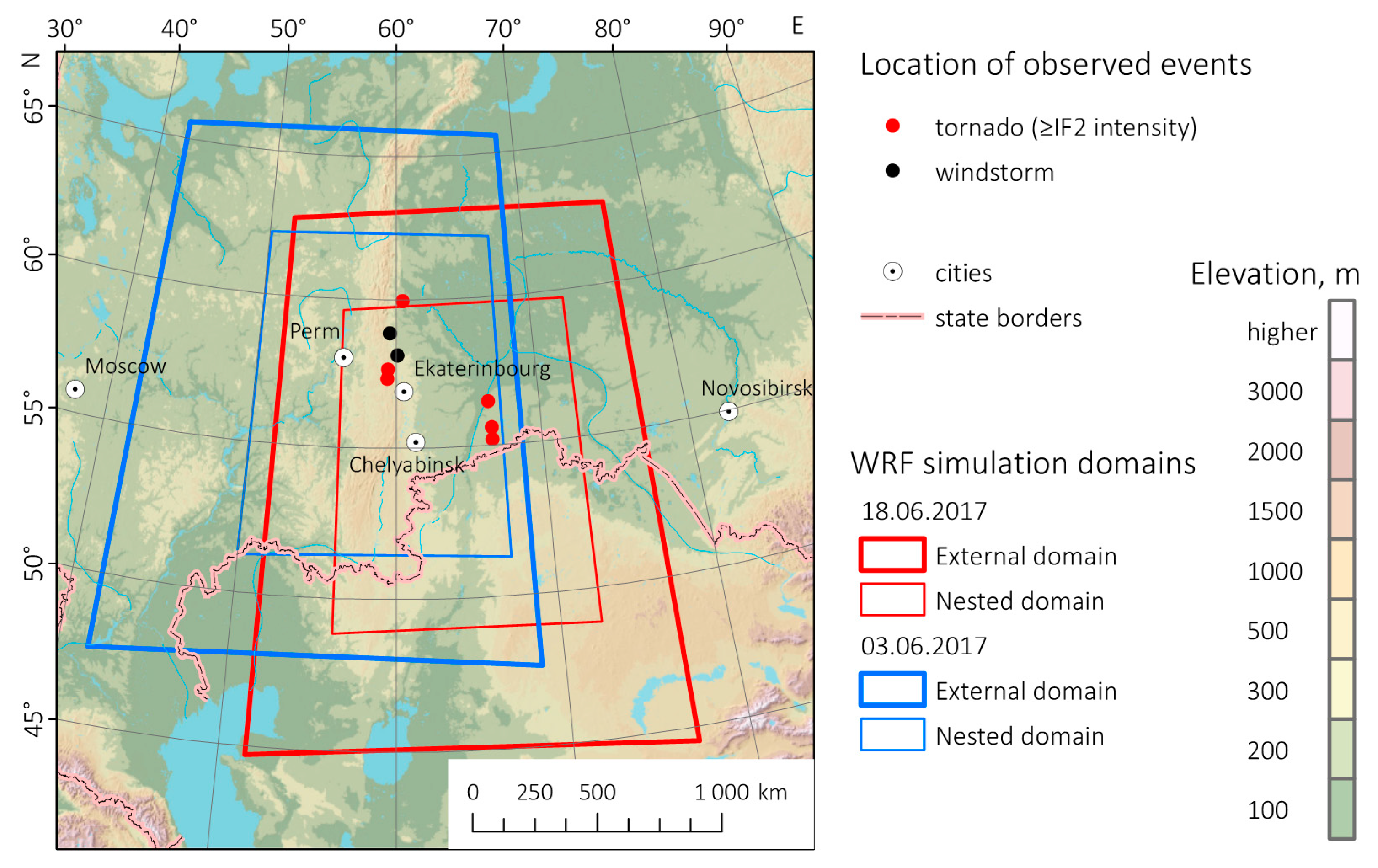
Figure 2.
Surface synoptic charts for (a) 1200 UTC 3 June 2017 and (b) 1200 UTC 18 June 2017. Red triangles indicate the point with strongest tornado observed.
Figure 2.
Surface synoptic charts for (a) 1200 UTC 3 June 2017 and (b) 1200 UTC 18 June 2017. Red triangles indicate the point with strongest tornado observed.
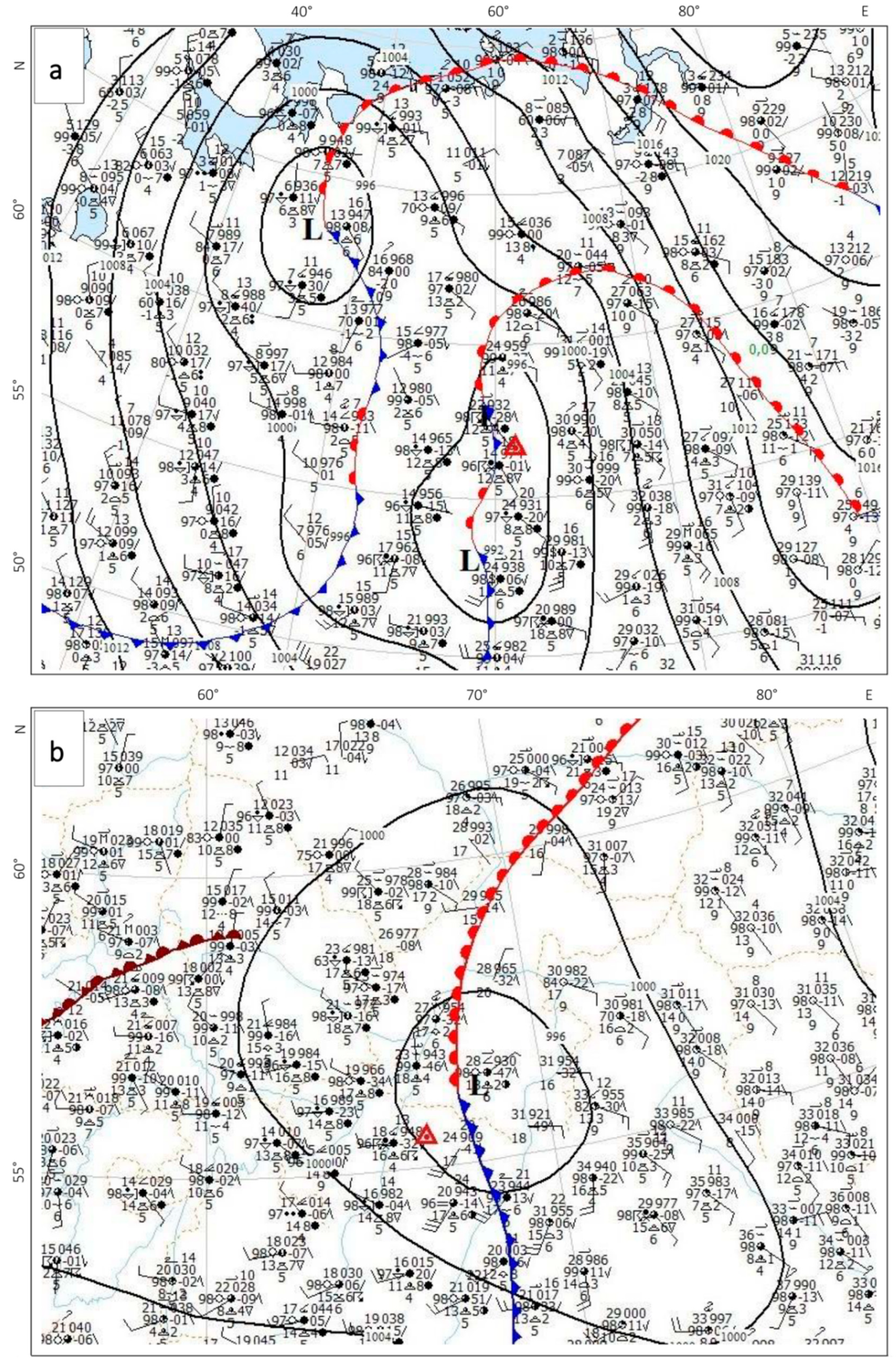
Figure 3.
Skew-T diagram at (a) 1200 UTC 3 June 2017 and (b) 0900 UTC 18 June 2017, obtained by the GFS/NCEP model forecasts for the coordinates of the observed tornadoes.
Figure 3.
Skew-T diagram at (a) 1200 UTC 3 June 2017 and (b) 0900 UTC 18 June 2017, obtained by the GFS/NCEP model forecasts for the coordinates of the observed tornadoes.
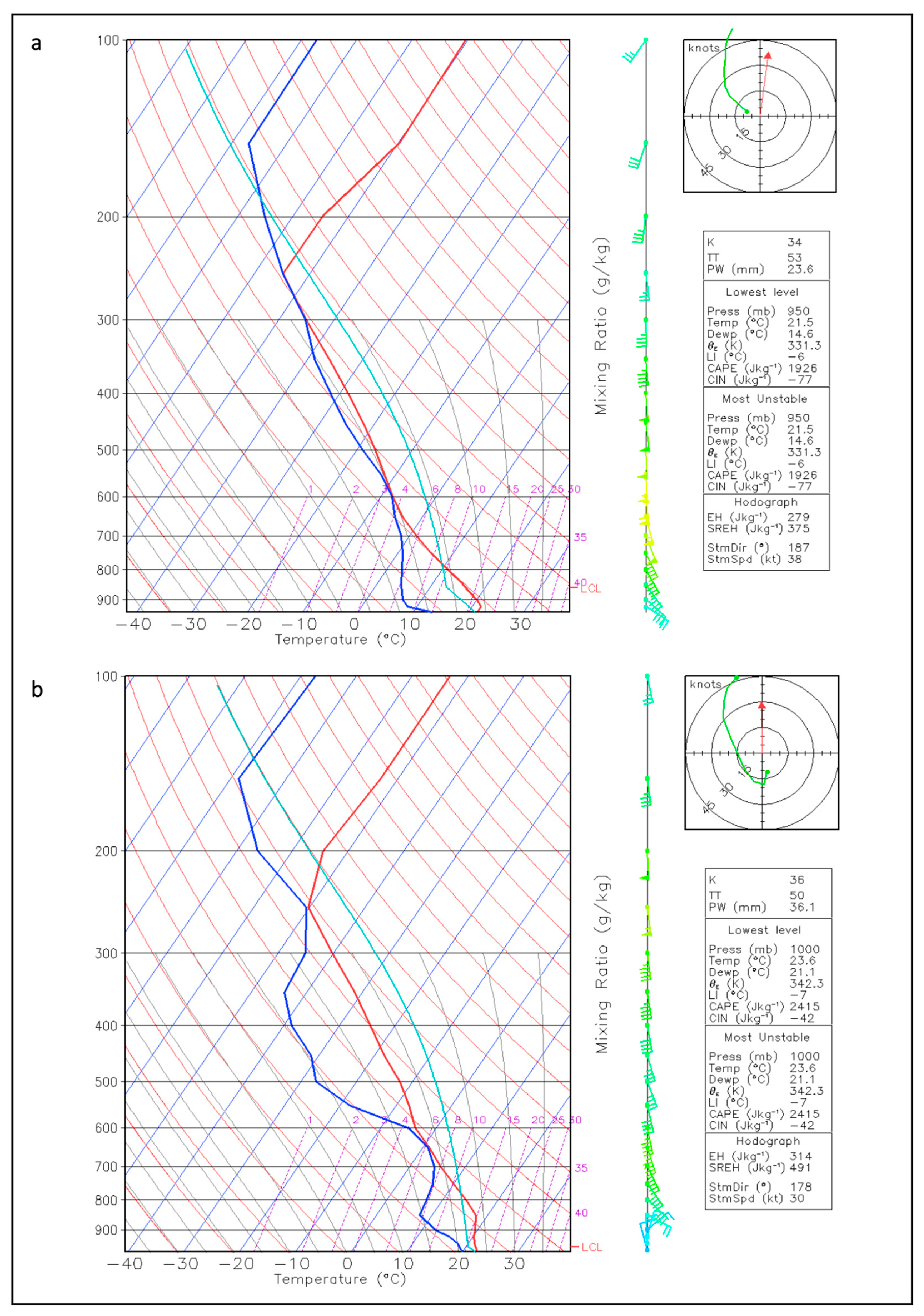
Figure 4.
The severe convective storm over the west of the Sverdlovsk region on the Meteosat-8 images: HRV cloud RGB images and IR10.8 channel data (CTT < −32 °C) at 1115 UTC (a,b) and 1145 UTC (c,d) of 3 June 2017. See also Supplementary Materials for animation.
Figure 4.
The severe convective storm over the west of the Sverdlovsk region on the Meteosat-8 images: HRV cloud RGB images and IR10.8 channel data (CTT < −32 °C) at 1115 UTC (a,b) and 1145 UTC (c,d) of 3 June 2017. See also Supplementary Materials for animation.

Figure 5.
Mescoscale convective complex over the Kurgan region on the Meteosat-8 image: (a) HRV cloud RGB image and (b) IR10.8 channel data (CTT < −32 °C) at 1130 UTC of 18 June 2017. See also Supplementary Materials for animation.
Figure 5.
Mescoscale convective complex over the Kurgan region on the Meteosat-8 image: (a) HRV cloud RGB image and (b) IR10.8 channel data (CTT < −32 °C) at 1130 UTC of 18 June 2017. See also Supplementary Materials for animation.
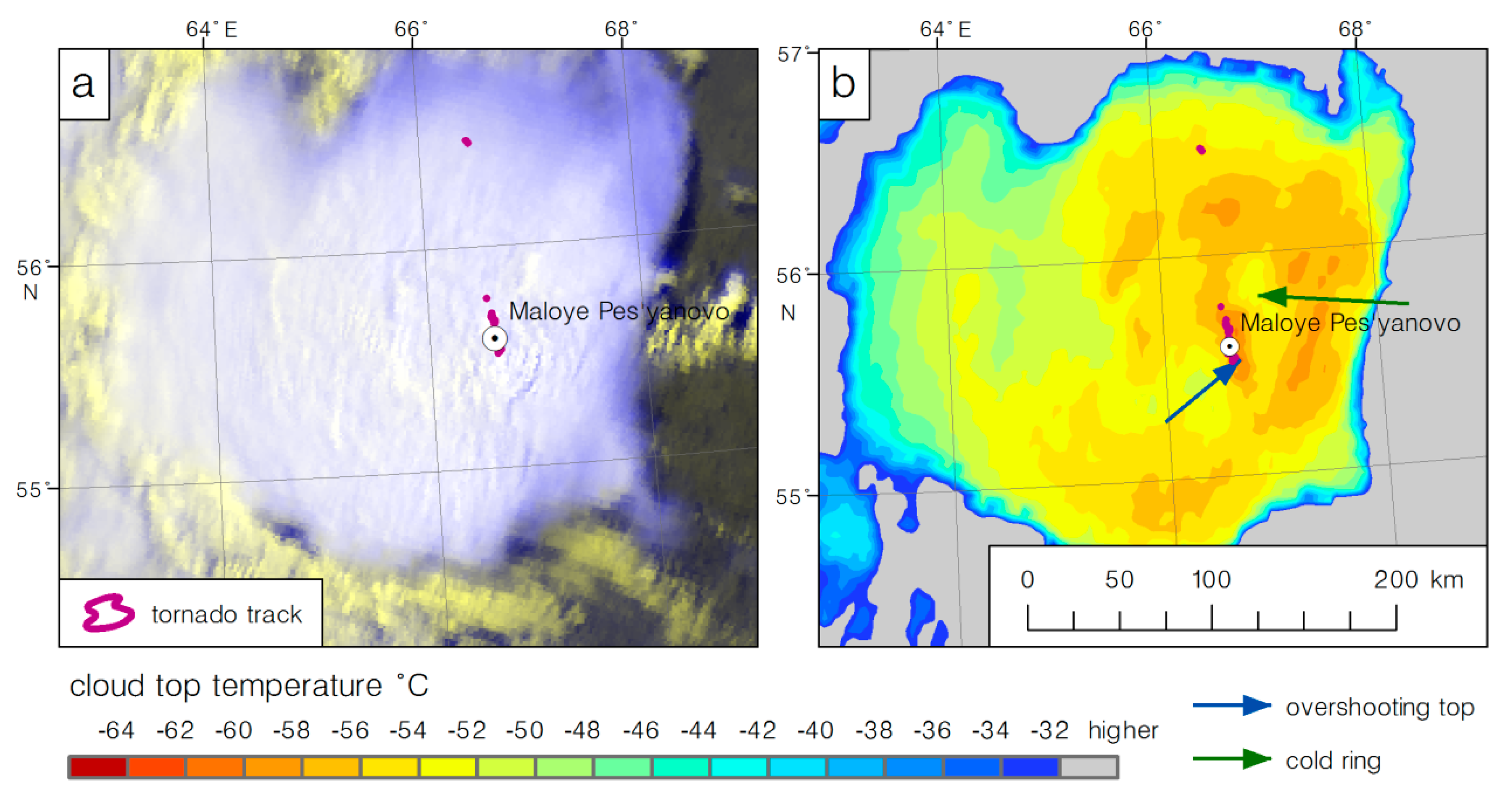
Figure 6.
Tornadoes and large-scale (>1 km2) windthrow events reported at 3 June 2017 and 18 June 2017 (the most probable intensity rating is shown).
Figure 6.
Tornadoes and large-scale (>1 km2) windthrow events reported at 3 June 2017 and 18 June 2017 (the most probable intensity rating is shown).
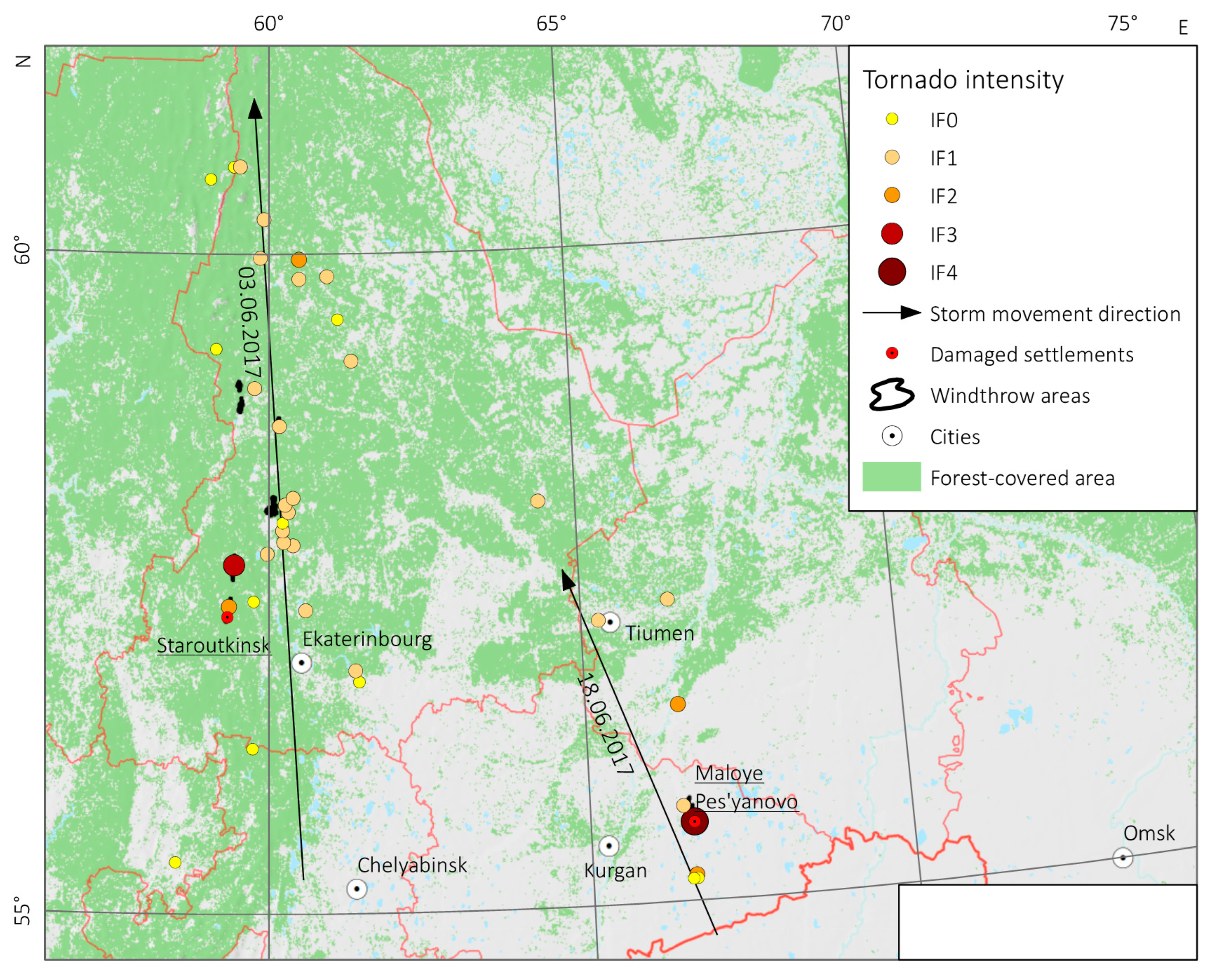
Figure 7.
Forest damage tracks caused by tornadoes of 3 June 2017 near Staroutkinsk (a) and Visim (b) settlements, and the high-resolution aerial image of wind-damaged forest (c) of the tornado track near Visim.
Figure 7.
Forest damage tracks caused by tornadoes of 3 June 2017 near Staroutkinsk (a) and Visim (b) settlements, and the high-resolution aerial image of wind-damaged forest (c) of the tornado track near Visim.
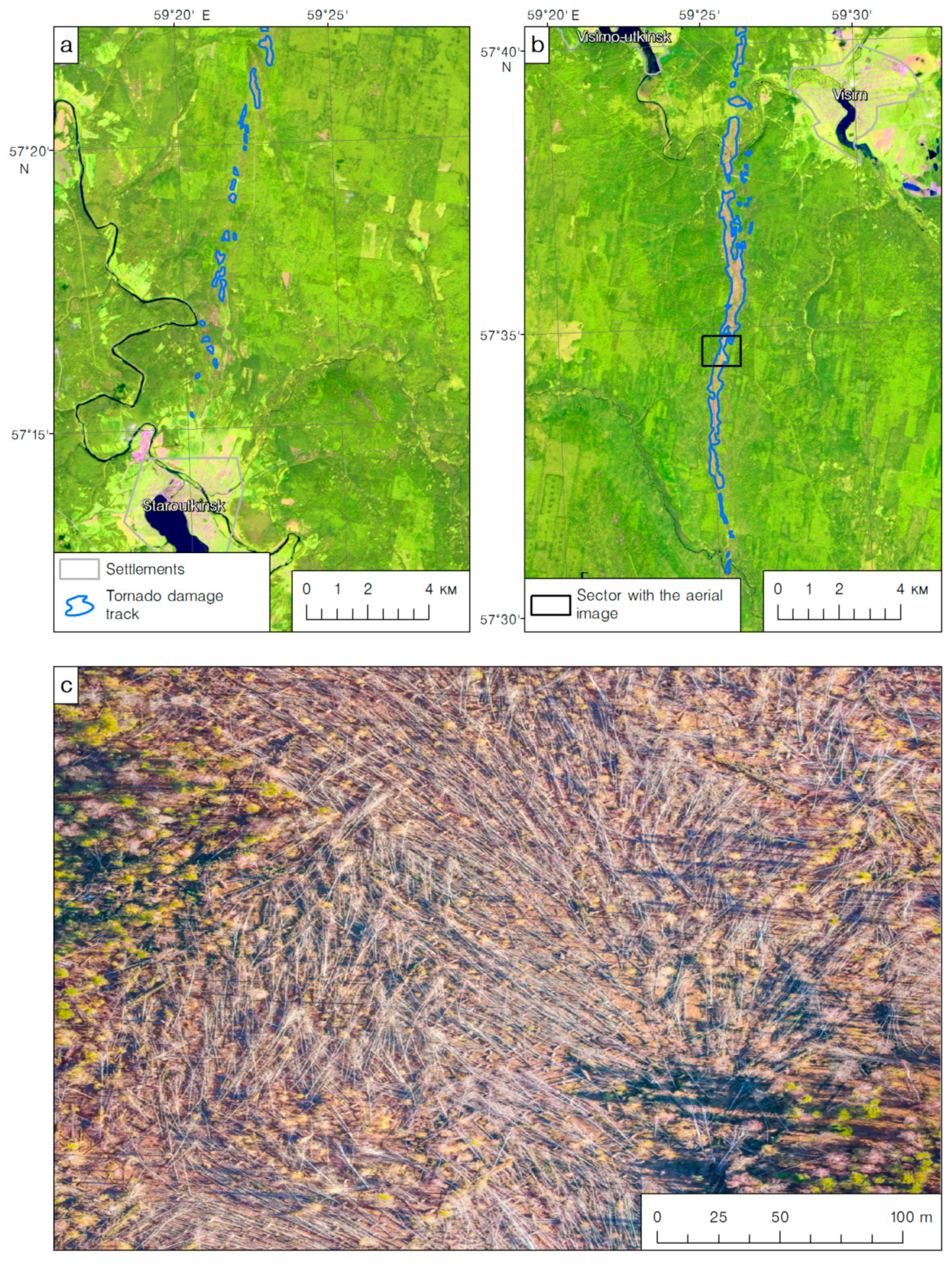
Figure 8.
Forest damage track caused by the IF4 tornado of 18 June 2017 passed through Maloye Pesyanovo village (a), high-resolution image of related damage in forest (b), and photo of destroyed log-houses and debarked tree in Maloe Pesynovo village (c).
Figure 8.
Forest damage track caused by the IF4 tornado of 18 June 2017 passed through Maloye Pesyanovo village (a), high-resolution image of related damage in forest (b), and photo of destroyed log-houses and debarked tree in Maloe Pesynovo village (c).
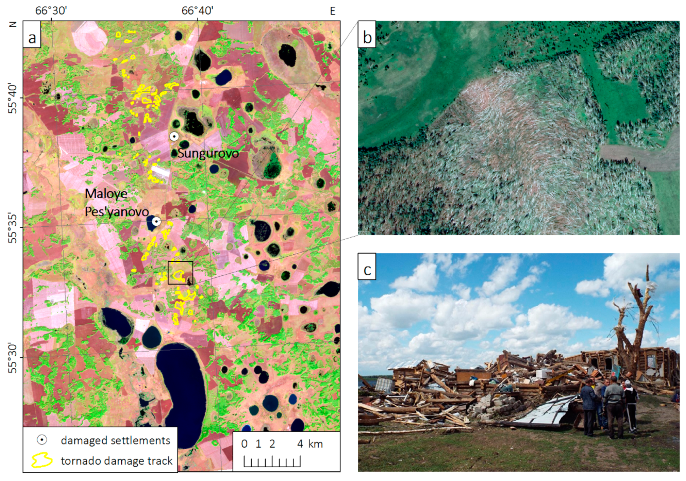
Figure 9.
WRF-simulated composite reflectivity (dBz), storm-relative helicity (m2 s−2), and wind gusts (m s−1) at 1200 UTC 3 June 2017 with different model grid resolution settings: 3 km with no nested grid (a), 7.2 km with no nested grid (b), and 9 km with 3-km nested grid (c).
Figure 9.
WRF-simulated composite reflectivity (dBz), storm-relative helicity (m2 s−2), and wind gusts (m s−1) at 1200 UTC 3 June 2017 with different model grid resolution settings: 3 km with no nested grid (a), 7.2 km with no nested grid (b), and 9 km with 3-km nested grid (c).

Figure 10.
WRF-simulated composite reflectivity (dBz), storm-relative helicity (m2 s−2), and wind gusts (m s−1) at 1300 UTC 18 June 2017 with various model grid resolution settings: 3 km with no nested grid (a), 7.2 km with no nested grid (b), and 9 km with 3-km nested grid (c).
Figure 10.
WRF-simulated composite reflectivity (dBz), storm-relative helicity (m2 s−2), and wind gusts (m s−1) at 1300 UTC 18 June 2017 with various model grid resolution settings: 3 km with no nested grid (a), 7.2 km with no nested grid (b), and 9 km with 3-km nested grid (c).
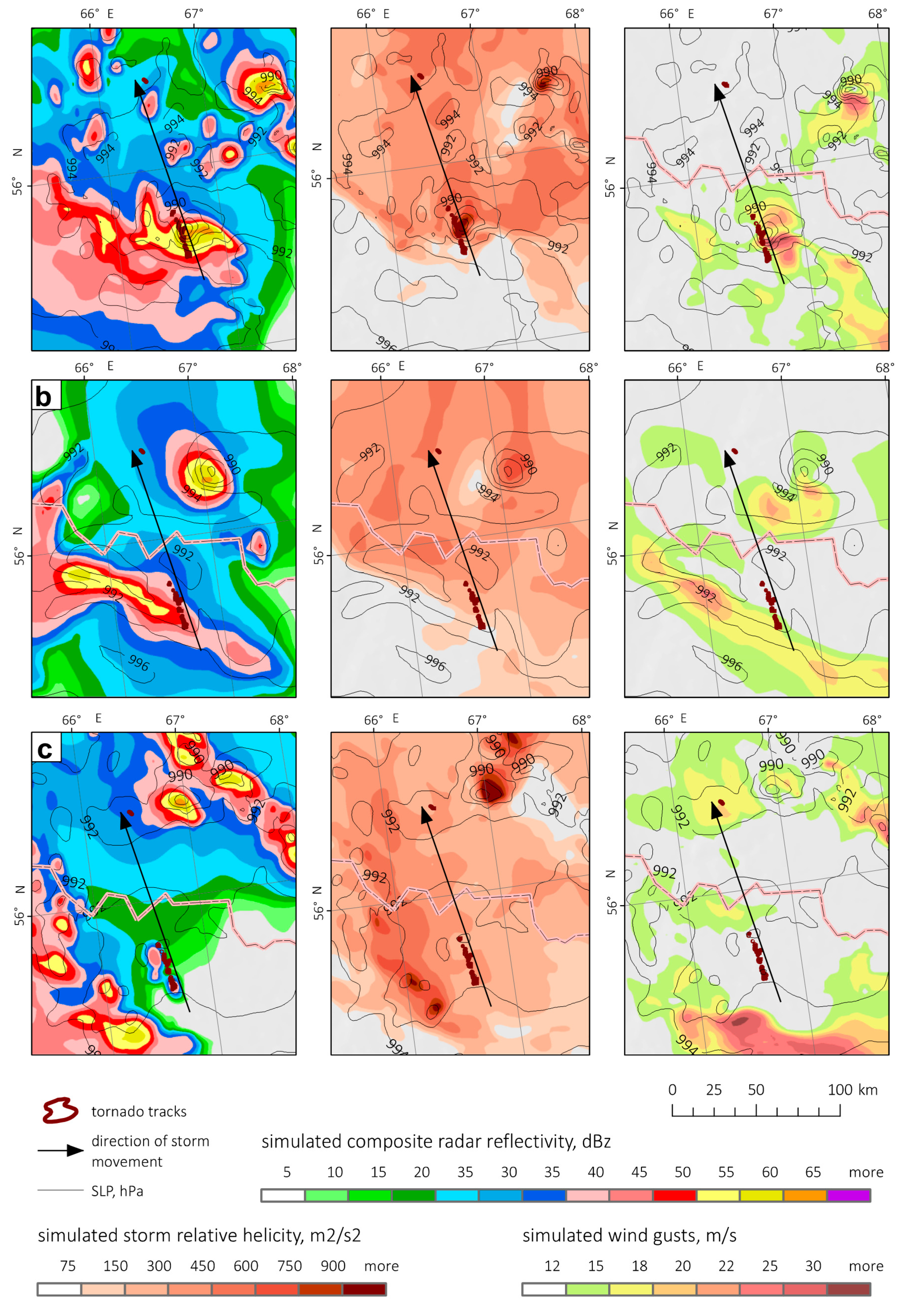
Figure 11.
HRV cloud RGB image (a) and cloud top temperature (b) by the Meteosat-8 data; WRF-simulated composite reflectivity (c) and cloud top temperature (d) at 1200 UTC 3 June 2017 (the WRF configuration with a 3-km resolution with no nested grid).
Figure 11.
HRV cloud RGB image (a) and cloud top temperature (b) by the Meteosat-8 data; WRF-simulated composite reflectivity (c) and cloud top temperature (d) at 1200 UTC 3 June 2017 (the WRF configuration with a 3-km resolution with no nested grid).
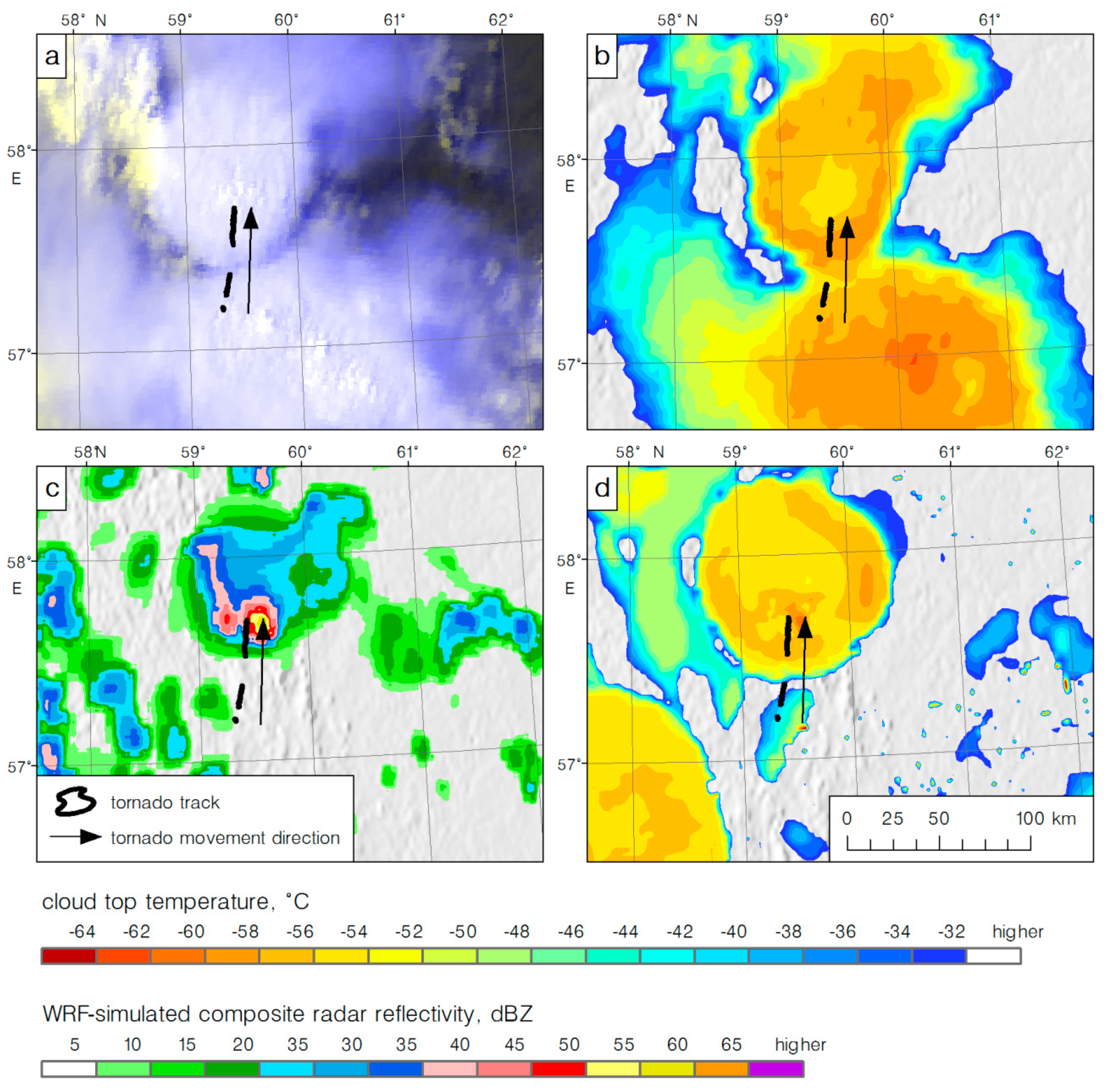
Figure 12.
HRV cloud RGB image (a) and cloud top temperature (b) by the Meteosat-8 data; WRF-simulated composite reflectivity (c) and cloud top temperature (d) at 1200 UTC 18 June 2017 (the WRF configuration with a 3-km resolution with no nested grid).
Figure 12.
HRV cloud RGB image (a) and cloud top temperature (b) by the Meteosat-8 data; WRF-simulated composite reflectivity (c) and cloud top temperature (d) at 1200 UTC 18 June 2017 (the WRF configuration with a 3-km resolution with no nested grid).
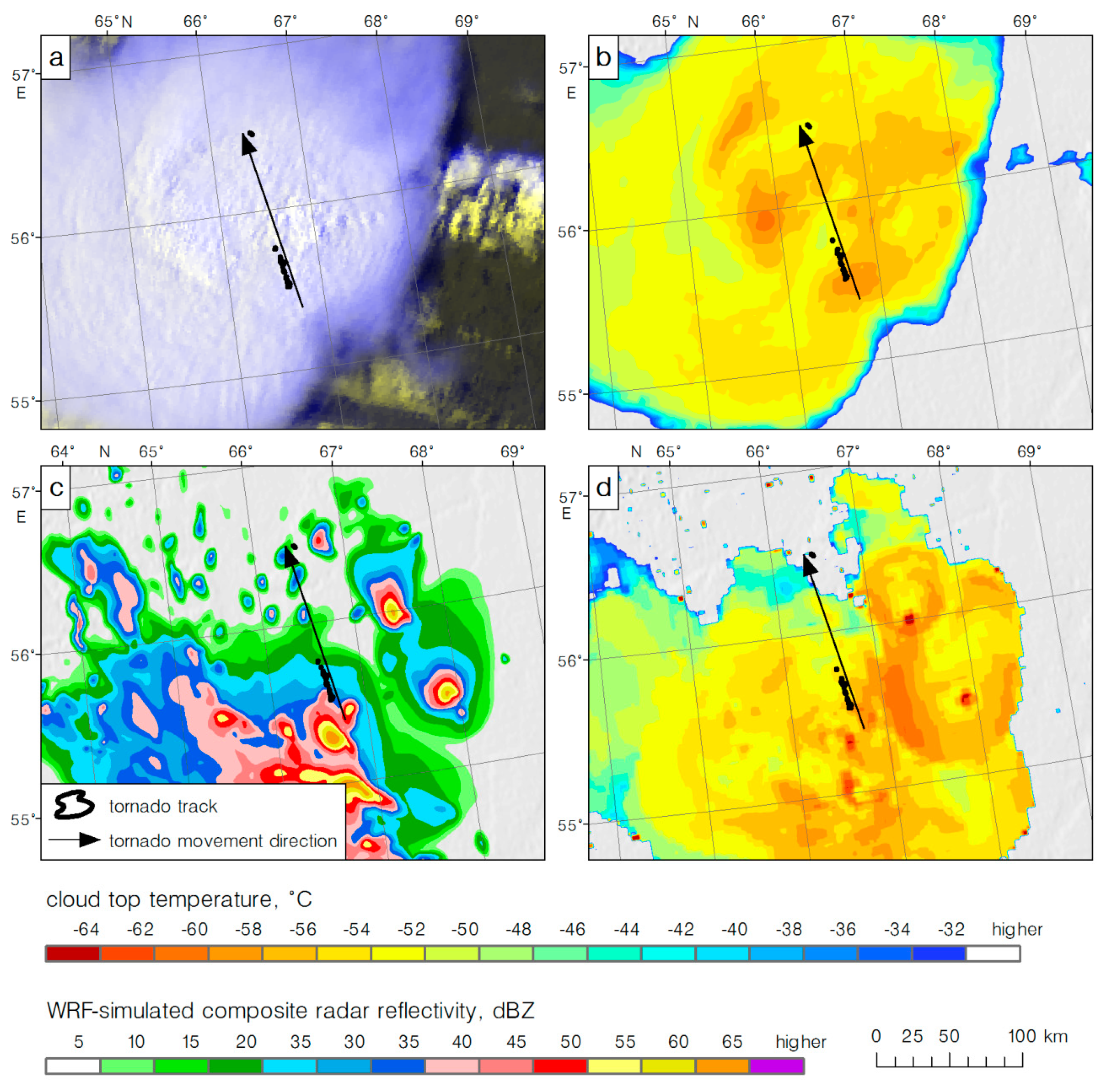
Figure 13.
WRF-simulated composite reflectivity (dBz), storm-relative helicity (m2 s−2), and wind gusts at 1200 UTC 3 June 2017 with the different forecast lead time: (a) model start time at 0000 UTC 2 June 2017 (the 36-h lead time) and (b) model start time at 1200 UTC 2 June 2017 (the 24-h lead time).

Table 1.
Summary of the WRF model settings.
| Model Characteristic | Setting |
|---|---|
| Horizontal grid resolution and grid points | 7.2 km/278 × 278 (with no nested grid) |
| 3 km/600 × 600 (with no nested grid) | |
| 9 km/333 × 333, with one nested grid (3 km/400 × 400) | |
| Number of vertical layers (up to 50 hPa) | 38 |
| Topography | U.S. Geological Survey (USGS) DEM (30 s) |
| Simulation length | 27 h, 39 h, 51 h (for the 12-, 24-, and 36-h lead time, respectively) |
| Output data time step | 1 h |
| Dynamics | Non-hydrostatic |
| Model core | Advanced Research WRF (ARW), non-hydrostatic |
| Integration time step | 48 s (for 9 km grid), 36 s (for 7.2 km grid), or 18 s (for 3 km grid) |
| Initial and lateral boundary | 0.25° GFS analysis and forecast |
| Microphysics schemes | Thompson scheme [71] |
| Planetary Boundary Layer (PBL) scheme | Yonsei University scheme [72] |
| Land surface physics scheme | Noah Land Surface Model [73] |
| Long- and short-wave radiation scheme | Rapid Radiative Transfer Model (RRTM) [74] |
| Surface layer scheme | Monin-Obukhov with Carslon-Boland viscous sub-layer and standard similarity functions [75] |
| Convection | Explicit (cloud-resolving) modeling |
Table 2.
Diagnostic variables calculated according to the GFS/NCEP (first line) and GEM/CMC (second line) model outputs (12-h forecasts from the 0000 UTC 3 June 2017 and 0000 UTC 18 June 2017, respectively). CIN and STP were obtained only for the GFS/NCEP data.
Table 2.
Diagnostic variables calculated according to the GFS/NCEP (first line) and GEM/CMC (second line) model outputs (12-h forecasts from the 0000 UTC 3 June 2017 and 0000 UTC 18 June 2017, respectively). CIN and STP were obtained only for the GFS/NCEP data.
| Date, Time | SB CAPE, J Kg−1 | SB CIN, J Kg−1 | SB LI, °C | LLS, m s−1 | DLS, m s−1 | WMAX SHEAR, m2 s−2 | 0–3 km SRH, m2 s−2 | EHI | SCP | STP |
|---|---|---|---|---|---|---|---|---|---|---|
| 3 June 2017, 1200 UTC | 2200 1800 | −127 — | −8 −4 | 7 15 | 4 8 | 450 100 | 480 360 | 4.2 2.5 | 0.8 0.4 | 2.5 — |
| 18 June 2017, 1200 UTC | 4200 3000 | −72 — | −12 −8 | 11 12 | 21 14 | 1203 480 | 450 560 | 3.4 5.0 | 3.5 3.4 | 2.9 — |
Table 3.
WRF-simulated characteristics of tornadic storms 3 June 2017 and 18 June 2017.
| Date, Time (UTC) | Model Grid Size (km) and Nested Grid (Y/N) Resolution | WRF-Simulated Storm Parameters (Maximum Values in 50-km Radius around a Tornado Track) | ||
|---|---|---|---|---|
| 0–3 km SRH, m2 s−2 | Composite Reflectivity, DBZ | Wind Gust Speed, m s−1 | ||
| 03.06.2017, 1100–1200 | 7.2, N | 1200 | 42 | 13 |
| 3, N | 1075 | 58 | 13 | |
| 9, Y (3) | 770 | 47 | - | |
| 18.06.2017, 1200–1300 | 7.2, N | 610 | 56 | 23 |
| 3, N | 1200 | 64 | 31 | |
| 9, Y (3) | 990 | 58 | 31 | |
Table 4.
Comparison of simulated storms characteristics with Meteosat-8 satellite data.
| Date, Time (UTC) | Model Grid Resolution (km) and Nested Grid (Y/N) Resolution | Minimum CTT, °C (Meteosat-8 data/WRF Model Forecast) | Distance between Observed and Simulated Storm Track, km | Timing Error, h |
|---|---|---|---|---|
| 03.06.2017, 1100–1200 | 7.2, N | −62/−61 | 40 | +1.25 |
| 3, N | −62/−61 | 10 | 0 | |
| 9, Y (3) | −62/−62 | 0 | −0.5 | |
| 18.06.2017, 1100–1200 | 7.2, N | −64/−62 | 35 | +1.5 |
| 3, N | −64/−64 | 10 | +1.5 | |
| 9, Y (3) | −64/−62 | 15 | +2.5 |
Table 5.
Characteristics of the severe storms with tornadoes 3 June 2017 and 18 June 2017, simulated by the WRF model with the 24- and 36-h forecast lead time.
Table 5.
Characteristics of the severe storms with tornadoes 3 June 2017 and 18 June 2017, simulated by the WRF model with the 24- and 36-h forecast lead time.
| Date, Time (UTC) | Model Start Date and Time (UTC) | WRF-Simulated Storm Parameters (Maximum Values in 50-km Radius around a Tornado Track) | ||
|---|---|---|---|---|
| 0–3 km Storm Relative Helicity (SRH), m2 s−2 | Composite Reflectivity, DBZ | Wind Gust Speed, m s−1 | ||
| 03.06.2017, 1100–1200 | 02.06.2017, 0000 | 1000 | 57 | 17 |
| 02.06.2017, 1200 | 1350 | 60 | 28 | |
| 03.06.2017, 0000 | 1075 | 58 | 13 | |
| 18.06.2017, 1200–1300 | 17.06.2017, 0000 | 600 | 52 | 30 |
| 17.06.2017, 1200 | 400 | 57 | 23 | |
| 18.06.2017, 0000 | 1200 | 64 | 31 | |
Table 6.
Comparison of the storm characteristics simulated by the WRF model (with the24- and 36-h forecast lead time) with the Meteosat-8 satellite data.
Table 6.
Comparison of the storm characteristics simulated by the WRF model (with the24- and 36-h forecast lead time) with the Meteosat-8 satellite data.
| Date, Time (UTC) | Model Start Date and Time (UTC) | Minimum Cloud Top Temperature, °C (Meteosat-8/WRF) | Distance between Observed and Simulated Storm Track, km | Timing Error, h |
|---|---|---|---|---|
| 03.06.2017, 1100–1200 | 02.06.2017, 0000 | −62/– | 50 | +1.25 |
| 02.06.2017, 1200 | −62/−64 | 15 | +1.5 | |
| 03.06.2017, 0000 | −62/−61 | 10 | 0 | |
| 18.06.2017, 1100–1200 | 17.06.2017, 0000 | −64/−61 | 50 | +1.25 |
| 17.06.2017, 1200 | −64/−62 | 35 | +1.0 | |
| 18.06.2017, 0000 | −64/−64 | 10 | +1.5 |
Publisher’s Note: MDPI stays neutral with regard to jurisdictional claims in published maps and institutional affiliations. |
© 2020 by the authors. Licensee MDPI, Basel, Switzerland. This article is an open access article distributed under the terms and conditions of the Creative Commons Attribution (CC BY) license (http://creativecommons.org/licenses/by/4.0/).
Share and Cite
MDPI and ACS Style
Chernokulsky, A.; Shikhov, A.; Bykov, A.; Azhigov, I. Satellite-Based Study and Numerical Forecasting of Two Tornado Outbreaks in the Ural Region in June 2017. Atmosphere 2020, 11, 1146. https://doi.org/10.3390/atmos11111146
AMA Style
Chernokulsky A, Shikhov A, Bykov A, Azhigov I. Satellite-Based Study and Numerical Forecasting of Two Tornado Outbreaks in the Ural Region in June 2017. Atmosphere. 2020; 11(11):1146. https://doi.org/10.3390/atmos11111146
Chicago/Turabian StyleChernokulsky, Alexander, Andrey Shikhov, Alexey Bykov, and Igor Azhigov. 2020. "Satellite-Based Study and Numerical Forecasting of Two Tornado Outbreaks in the Ural Region in June 2017" Atmosphere 11, no. 11: 1146. https://doi.org/10.3390/atmos11111146
Note that from the first issue of 2016, this journal uses article numbers instead of page numbers. See further details here.