Article

The Impact of Ensemble Meteorology on Inverse Modeling Estimates of Volcano Emissions and Ash Dispersion Forecasts: Grímsvötn 2011

1
Department of Meteorology, University of Reading, Reading RG6 6BB, UK
2
Met Office, FitzRoy Road, Exeter EX1 3PB, UK
3
College of Engineering, Mathematics and Physical Sciences, University of Exeter, Exeter EX4 4QF, UK
4
COMET, Sub-Department of Atmospheric, Oceanic and Planetary Physics, University of Oxford, Oxford OX1 3PU, UK
5
Sub-Department of Atmospheric, Oceanic and Planetary Physics, University of Oxford, Oxford OX1 3PU, UK
*
Author to whom correspondence should be addressed.
Atmosphere 2020, 11(10), 1022; https://doi.org/10.3390/atmos11101022
Submission received: 12 August 2020 / Revised: 17 September 2020 / Accepted: 18 September 2020 / Published: 23 September 2020
(This article belongs to the Special Issue Forecasting the Transport of Volcanic Ash in the Atmosphere)

Abstract

:
Volcanic ash can interact with the earth system on many temporal and spatial scales and is a significant hazard to aircraft. In the event of a volcanic eruption, fast and robust decisions need to be made by aviation authorities about which routes are safe to operate. Such decisions take into account forecasts of ash location issued by Volcanic Ash Advisory Centers (VAACs) which are informed by simulations from Volcanic Ash Transport and Dispersion (VATD) models. The estimation of the time-evolving vertical distribution of ash emissions for use in VATD simulations in real time is difficult which can lead to large uncertainty in these forecasts. This study presents a method for constraining the ash emission estimates by combining an inversion modeling technique with an ensemble of meteorological forecasts, resulting in an ensemble of ash emission estimates. These estimates of ash emissions can be used to produce a robust ash forecast consistent with observations. This new ensemble approach is applied to the 2011 eruption of the Icelandic volcano Grímsvötn. The resulting emission profiles each have a similar temporal evolution but there are differences in the magnitude of ash emitted at different heights. For this eruption, the impact of precipitation uncertainty (and the associated wet deposition of ash) on the estimate of the total amount of ash emitted is larger than the impact of the uncertainty in the wind fields. Despite the differences that are dominated by wet deposition uncertainty, the ensemble inversion provides confidence that the reduction of the unconstrained emissions (a priori), particularly above 4 km, is robust across all members. In this case, the use of posterior emission profiles greatly reduces the magnitude and extent of the forecast ash cloud. The ensemble of posterior emission profiles gives a range of ash column loadings much closer in agreement with a set of independent satellite retrievals in comparison to the a priori emissions. Furthermore, airspace containing volcanic ash concentrations deemed to be associated with the highest risk (likelihood of exceeding a high concentration threshold) to aviation are reduced by over 85%. Such improvements could have large implications in emergency response situations. Future research will focus on quantifying the impact of uncertainty in precipitation forecasts on wet deposition in other eruptions and developing an inversion system that makes use of the state-of-the-art meteorological ensembles which has the potential to be used in an operational setting.

1. Introduction

Volcanic ash, released into the atmosphere when a volcano explosively erupts, provides a significant hazard to aircraft as it can cause engines to malfunction and visibility can be reduced by external corrosion. It can also cause permanent engine damage which leads to high maintenance costs [1]. Grounding and re-routing of aircraft during an eruption also comes with a large economic cost. For example, the eruption at the summit of the Icelandic volcano Eyjafjallajökull in April 2010 disrupted European airspace for 13 days, grounded over 95,000 flights and is estimated to have cost the airline industry over £1 billion [2]. The aim of this paper is to present a method that optimally combines satellite retrievals and ensemble numerical weather prediction simulations to produce improved ash forecasts that can be used by the aviation industry during future volcanic eruptions.
In the event of an eruption, one of the nine worldwide Volcanic Ash Advisory Centers (VAACs) issue hazard maps forecasting horizontal ash coverage in three vertically integrated layers of the atmosphere at 6 h intervals to a maximum forecast lead time of 18 h. The ash forecasts show the maximum expected extent of the ash cloud within 3 flight level ranges but contain no quantitative information about ash concentration. These forecasts aid the aviation community in making decisions to minimize the risk of encountering ash during their flight operations. Before the 2010 Eyjafjallajökull eruption, the International Civil Aviation Organization (ICAO) guidelines were to avoid all ash [3]. However due to the unprecedented disruption in 2010, the United Kingdom’s Civil Aviation Authority (CAA), in consultation with Rolls-Royce, the UK Met Office, international and European regulators, and aviation experts developed quantitative peak concentration limits [4,5]. The UK Met Office, who host the London VAAC, also began producing quantitative peak concentration forecasts for the North Atlantic and European areas during an eruption using the Numerical Atmospheric-Dispersion Modeling Environment (NAME), a Lagrangian particle dispersion model. The concentration thresholds that are currently used in the production of these forecasts are high (>4000 μ g m 3 ), medium (2000–4000 μ g m 3 ) and low (200–2000 μ g m 3 ) ash contamination. Before aircraft are permitted to fly in regions of medium and high ash contamination, operators are required to have a safety risk assessment approved by their national aviation authority [6,7]. ICAO guidelines are periodically under review and therefore there is the potential for procedural change in the future. A possible change is the need for all VAACs to issue quantitative ash concentration forecasts with predefined concentration thresholds. This is currently difficult due to the large uncertainty associated with volcanic emissions, particularly for remote locations with limited in situ observations.
The forecasting of ash location following an eruption is performed by the VAACs using volcanic ash transport and dispersion (VATD) models and is strongly dependent on information about the eruption that is used for initialization e.g., [8,9,10]. Information about the height of the plume, the mass eruption rate, the eruption duration and the particle size distribution is required. Eruption duration can be monitored by satellite or using estimates from observers in the locality and there are a variety of techniques to estimate the height of the plume e.g., [11]. Empirical relationships based on past eruptions e.g., [12,13] are typically used to estimate a mass eruption rate from the reported plume height. These empirical relationships do not account for the influence of the meteorological situation (e.g., wind bent plumes [14]) and a uniform vertical distribution of ash from the volcano vent to the reported plume height is typically assumed by the London VAAC.
VATD models also use meteorological information as input, including forecast 3-dimensional wind fields, precipitation and meteorological cloud location from numerical weather prediction models as input. This meteorological information governs the transport and dispersion of the ash cloud and the removal of ash from the atmosphere via deposition. The effect of smaller scale motions, not represented in the input meteorology, is parametrized within the VATD model. Current operational VATD models use only one realization of the meteorological situation, known as a deterministic forecast. Uncertainties in the synoptic situation are therefore not considered in the resulting forecasts and this can result in errors in the forecast ash cloud position [8]. This variability can be represented if an ensemble of meteorological forecasts are used as input for VATD models. Despite being advocated by the volcanic ash community as a way for accounting for wind and precipitation uncertainty [15,16], ensemble meteorology is not routinely used to produce ash forecasts. Barriers to the use of the state-of-the-art ensemble science include the need for forecasts to be produced within a short time window and the ability to present ensemble results in a way that can be easily used by decision makers [17].
A small number of studies have investigated the impact of ensemble meteorology on volcanic ash forecasts. Dare et al. [18] found that there is better agreement with satellite observations if an ensemble is used compared to a single realization of the meteorological situation for lead times greater than 12 h. More recent work by Zidikheri et al. [19] found that using an ensemble of dispersion model simulations with different meteorological fields obtained from an ensemble meteorological forecast model and different values of ash source parameters gave increased Brier skill scores at all lead times compared to a deterministic forecast. This is relevant as the current volcanic ash advisories and graphics produced by the VAACs are issued out to 18 h. Studies by Stefanescu et al. [20] and Madankan et al. [21] concluded that at longer lead times (48 h) there can be a large spread in predicted ash concentrations within forecasts made using ensemble meteorology. This large spread often occurs when ash particles encounter regions of large horizontal flow separation in the atmosphere. Nearby ash particle trajectories can rapidly diverge, leading to a reduction in the forecast accuracy of deterministic forecasts that do not represent uncertainty in wind fields at the synoptic scale [22]. Precipitation uncertainty can also impact ash forecast accuracy. In the case study presented in Langmann et al. [23] it was found that wet deposition, the removal of ash through microphysical processes, can remove up to 23% of ash, consistent with [18] which found that wet deposition removed 1–30% of ash, depending on the season.
Satellite observations show the extent of the ash cloud and can give estimates of ash column loading, ash cloud top height and effective ash radius e.g., [24,25]. Satellite retrievals can be combined with a dispersion model using an inversion technique to give time-evolving estimates of mass eruption rate, and the vertical distribution of the ash emissions from the eruptive plume. These quantities are not directly retrievable from satellites. There are numerous published methodologies that use inversion modeling to estimate ash [26,27,28,29,30,31] and sulfur dioxide (SO 2 ) [32,33,34,35,36,37,38] source parameters for volcanic eruptions. For example, the technique described in [29] is used in an operational framework by the London VAAC, where posterior estimates of emissions can be determined in near-real time as more satellite retrievals become available. However, all these methods make use of deterministic meteorological information, therefore errors in the wind fields or location of precipitation will lead to errors in the estimated source emissions.
This study brings together inversion modeling and the use of an ensemble of meteorological forecasts to give an ensemble of the most probable source emission estimates of volcanic ash that will undergo long range transport and therefore a robust ash forecast constrained by observations. This follows work by Zidikheri et al. [19] that addresses the problem of verifying and calibrating ensemble-based probabilistic volcanic ash forecasts using dispersion model simulations with different meteorological fields obtained from an ensemble meteorological forecast model and different values of ash source parameters. Zidikheri and Lucas [39] use an inversion modeling procedure involving an ensemble of meteorological forecasts to estimate fine ash mass emission rates and other source parameters for 14 eruption case studies.The ensemble forecasts used here as meteorological input to NAME are produced using the European Centre for Medium-Range Weather Forecasts (ECMWF) ensemble prediction system [40]. The NAME dispersion simulations will be used with satellite retrievals in the Inversion Technique for Emission Modeling (InTEM) system [29] that has been developed at the UK Met Office, to produce an ensemble of volcanic ash source emission terms. The impact of using the ensemble of emission source profiles on the resulting forecasts of ash location will be investigated for the 2011 Grímsvötn eruption, with a particular focus on regions where medium and high levels of ash contamination are predicted as these are areas that aircraft may be prohibited from entering.
The methods used to create the ash forecasts presented in this study are described in Section 2. Section 3 describes the details of the 2011 Grímsvötn eruption, the meteorological situation, the satellite observations of the ash and SO 2 cloud and the issued VAAC graphics. The impact of the use of ensemble meteorology on volcanic emission estimates and on flight planning decisions is presented in Section 4 and Section 5. The summary and conclusions of the study are in Section 6.

2. Methods and Data

2.1. Ensemble of Meteorological Forecasts

In this study, NAME is driven by a set of bespoke ensemble meteorological datasets over the Grímsvötn eruption period produced using the ECMWF Integrated Forecast System (IFS) (cycle 41r1). To account for uncertainty in the initial meteorological fields and therefore the resulting numerical weather prediction (NWP) forecasts, the ECMWF IFS Ensemble Prediction System (EPS) was used to produce a 20-member meteorological ensemble. The EPS uses the singular-vector approach [41] to perturb initial conditions in the meteorology and a stochastic physics scheme [42] to account for model uncertainty. These global forecasts are initialized every 24 h between 0000 UTC 21 May and 0000 UTC 26 May 2011 and have a forecast lead time of 72 h. Data are extracted from the ECMWF archive at 0.25 × 0.25 on a regular latitude/longitude grid, and the precipitation, surface stresses and sensible heat flux fields were post-processed so they can be used as input for NAME.

2.2. Satellite Observations

2.2.1. SEVIRI

The Spinning Enhanced Visible and InfraRed Imager (SEVIRI) is mounted on the geosynchronous Meteosat Second Generation (MSG) satellite. It has 12 spectral channels and provides high temporal (15 min) and spatial (3 km resolution at the equator) observations. The high temporal and spatial resolution makes these observations ideally suited to evaluate the transport of volcanic ash following an eruption. The volcanic ash measurements used in this paper are retrieved using the algorithm of [24] which uses three long-wave window channels centered at 8.7, 10.8, and 12.0 μ m to discriminate between meteorological cloud and ash cloud. Where ash is detected this algorithm determines the ash column loading. These pixels are flagged as containing ash. If a pixel is free from both ash and meteorological cloud then it is flagged as a clear sky pixel. Pixels that neither have detectable ash nor are flagged as clear skies are unclassified.
Further processing is performed to regrid the retrieved column loadings on to a grid of 0.375 latitude by 0.5625 longitude (approximately 40 km × 40 km in mid-latitudes) and averaged over 1 h. This is to match the resolution of the NAME ash concentration output and to reduce data volumes. If 50% or more satellite pixels in a grid box contain ash or more than 90% of pixels are classified as ash or clear skies, then the grid box is selected for use in the InTEM inversion. If all classified pixels within a grid box are flagged as clear sky pixels then the grid box is deemed to be a clear sky observation. Otherwise, the grid box is deemed to be an ash grid observation with the column loading in this grid box given by the mean of all the classified pixels (including clear skies). More information about the processing of the SEVIRI retrievals can be found in [43]. These processed retrievals are used with InTEM as an observational constraint on the inverted emissions profile.

2.2.2. IASI

The Infrared Atmospheric Sounding Interferometer (IASI) is in a sun-synchronous polar orbit on Metop-A, Metop-B and Metop-C [44]. It has a swath width of 2200 km with 12 km circular pixels at nadir. It achieves near global coverage every 12 h. It has 8461 channels with wavelengths in 645 to 2760 cm 1 which covers 3 SO 2 absorption bands [45] and the broad v-shaped absorption feature associated with volcanic ash at 750 and 1250 cm 1 [46]. There are several retrievals for SO 2 and ash developed for the IASI instrument e.g., [46,47,48,49,50,51,52,53]. The retrievals of SO 2 and ash for the Grímsvötn eruption presented in Figure 1 are determined using optimal estimation schemes developed by [50,52]. The ash retrieval used an ash refractive index measured by Reed et al. [54] from a sample of ash from the Grímsvötn eruption. IASI retrievals of ash and SO 2 are used in the description of the Grímsvötn 2011 case study investigated in this paper (Section 3).

2.2.3. MODIS

The Moderate Resolution Imaging Spectroradiometer (MODIS) is mounted on the NASA Terra and Aqua satellites. It is in a near-polar, sun-synchronous orbit. It has 36 spectral channels in the visible to infrared range (0.4 μ m to 14.4 μ m wavelength), a spatial resolution of 250–1000 m and global coverage every 1–2 days [55]. Here the Aqua MODIS calibrated and geolocated radiances data are used [56] and the Optimal Retrieval of Aerosol and Cloud (ORAC) retrieval algorithm is used to determine volcanic ash properties [57,58]. MODIS ash retrievals during the Grímsvötn eruption are used as independent satellite retrievals to evaluate NAME simulations of ash location and column loading.

2.3. VATD Model: NAME

To simulate the dispersion of volcanic ash, the VATD model NAME [59] was used. NAME includes parameterizations of turbulence, sedimentation, dry deposition and wet deposition, which are required to simulate the dispersion and removal of volcanic ash. Ash particles are typically assumed to have a density of 2300 kg m 3 , (although in reality density depends on chemical composition, porosity and grain size). Please note that aggregation of ash particles, near source plume rise and processes driven by the eruption dynamics (e.g., [14]) are not explicitly modeled in the operational configuration used by the London VAAC [16]. The particle size distribution used is based on data from [60].

2.4. Inversion System: InTEM

The inversion system used in this study is InTEM for volcanic ash which uses a Bayesian approach to estimate volcanic ash source parameters using satellite retrievals combined with dispersion modeling and an a priori estimate of the emission. This system has been developed at the UK Met Office (see [29] for full details) and was originally developed to estimate greenhouse gas emissions [61]. Using these input data, it provides a best estimate of the emissions profile for fine ash that can undergo long range dispersion. This emission profile has a chosen vertical resolution of 4 km and a time resolution of 3 h. The emissions profile can either be determined using satellite retrievals of ash only or of both ash and clear skies.

2.4.1. VATD Simulations

NAME simulations representing a nominal release rate (1 g s 1 ) from each possible source term component (4 km height range and 3-hourly time period) are conducted. Model predictions of ash column loads can be easily determined for an arbitrary emission profile by a linear combination of these nominal simulations. Only ash particles with diameters less than 30 μ m are included in these simulations. This assumption is similar to that made in Stohl et al. [34] that state SEVIRI retrievals have a preferential sensitivity to ash with particle diameters from 2 to 32 μ m.

2.4.2. Estimate of the Source Term a Priori

An a priori estimate of the source term is used to ensure that the inverted source term is not over fitted to the satellite observations but is also guided by known information concerning the eruption (e.g. eruption time, maximum plume height). The mean and error covariance matrix of the a priori are estimated using a stochastic model that includes correlations between errors in the a priori source term emissions at different heights and times. A uniform emission profile from the volcano vent to the plume height is assumed and errors in the observed plume height (assumed to be ± 2 km), in the assumed uniform emission profile and in the empirical relationship used to determine the mass eruption rate for a given plume height [12] are considered. A full description of the determination of the a priori source term used in the inversion process is given in [43]. In this study, the a priori source term is based on radar-recorded plume height which is combined with expert interpretation of other observations by the Icelandic Met Office State Volcano Observatory to provide an estimation of plume height.

2.4.3. The Inversion Algorithm

The inversion scheme yields a best estimate of the emission profile using the NAME simulations, SEVIRI retrievals and a priori estimate described above. The posterior distribution of emissions is Gaussian, and the best estimate of the emissions is taken as the peak of this distribution subject to a non-negative constraint. This best estimate of the emissions can then be used in forecasting the volcanic ash cloud. To find this peak, a cost function, which represents the simultaneous fit of the model ash loadings to the satellite retrievals and of the emissions to the a priori estimate, is minimized. The minimization is performed using the Lawson and Hanson non-negative least squares algorithm [62]. This algorithm is iterative (but fast) and converges completely in a finite number of iterations. Webster et al. [63] states that inversion run time for using 88791 satellite observations until 00:00 UTC on 31 May 2011 from the 2011 Grímsvötn eruption was 1 min 5 s. A full description of the inversion method is given in [29,43]. Please note that it is possible that there are significant uncertainties introduced by selecting the peak of posterior distribution but that is not the focus of this study.

3. Grímsvötn 2011: Case Study Description

The case study chosen to demonstrate the ensemble inversion method is the 2011 Grímsvötn eruption. Grímsvötn is located at 64.42 N, 17.33 W and has a vent height of 1719 m above sea level (asl). It is one of Iceland’s most active volcanoes and its most recent explosive eruption started at 1913 UTC on 21 May 2011 and had an initial eruptive plume height of 20–25 km asl [11]. The eruption lasted approximately 3 days and ended at 0230 UTC on 25 May 2011. Throughout the eruption period the eruptive plume height varied substantially between 2 and 20 km asl [11]. There is some evidence to suggest that there was a (or several) partial column collapse(s) leading to the compression of the lower part of the ash column, and a mechanism for driving a gravity current of ash outwards from the eruption column [64]. It is possible that this column collapse, which cannot currently be represented in VATD models, led to the SO 2 and ash clouds experiencing different atmospheric wind speeds and directions leading to errors in the forecasting of ash in northern Europe. This separation is clearly seen in Figure 1 which shows the maximum retrieved SO 2 (Figure 1a) and ash column loadings (Figure 1b), from IASI, travelling in different directions away from Grímsvötn.
Figure 2 shows the synoptic situation at 0000 UTC on 22 May 2011. There is a mature low-pressure system to the south-east of Iceland (992 hPa), with another developing cyclone following in the north Atlantic (1005 hPa). At low levels, the flow around these features would transport low level ash and SO 2 , emitted from the eruption, south-eastwards towards the UK. Analysis of the Skew-T thermodynamic chart from Keflavik radiosonde station at 0000 UTC on 22 May (not shown) indicates a large amount of vertical wind shear. The upper-level wind direction suggests that ash and SO 2 emitted above approximately 9 km would be transported northwards—the opposite direction to low level material. The meteorological situation remains similar for the duration of the eruption. The deepest system during the eruption had a central pressure of 977 hPa and moved north of Scotland overnight on 23/24 May. It was associated with strong north-westerly winds near the surface and heavy precipitation [65]. Beckett et al. [16] states that NWP forecast errors associated with these low-pressure systems led to the operational NAME simulations forecasting the ash cloud further south than observed and [66] suggests that precipitation over most of northern and central Europe might have caused a significant removal of ash due to wet deposition. The use of ensemble meteorology in this study will enable the investigation of uncertainties in the ash cloud position and in ash column loads associated with errors in the wind and precipitation fields.
Figure 3 shows two volcanic ash advisory graphics for (a) 1800 UTC on 23 May 2011 and (b) 0000 UTC on 25 May taken from the London VAAC: Volcanic ash advisories and graphics archive [67]. These graphics show an ash cloud extending northwards and then eastwards towards the Arctic and another branch extending south, travelling cyclonically towards western Europe. When bringing together the information from the IASI satellite retrievals (Figure 1) and the Met Office surface analysis chart (Figure 2), it seems likely that this north-eastward travelling branch of the forecast cloud may have been dominated by SO 2 emitted at a greater height than the ash. This is consistent with the findings of Moxnes et al. [38] and Cooke et al. [68] and surface observations of ash in many regions of Europe [65,66,69,70,71]. Pelley et al. [29] shows that the InTEM inversion, using a single realization of the meteorological situation, can distinguish between ash emitted at different altitudes and hence produces an emission profile that emits ash at lower altitudes than the a priori vertical distribution. This emission profile results in a forecast ash cloud that is consistent with the location of the ash, not SO 2 . In this study, the uncertainty in the posterior emission profile will be estimated by performing an ensemble of inversions using an ensemble of meteorological conditions.

4. Results

4.1. Posterior Inversion Estimates

Figure 4 shows the posterior height-time ash emission rates (g/h) obtained using InTEM for the Grímsvötn eruption (21–25 May 2011) using each of the EPS meteorological ensemble members with SEVIRI retrievals of ash and clear skies. Each panel shows the ash emission rates determined by InTEM using a single member of the EPS ensemble and the emission rates have a temporal resolution of 3 h and a vertical resolution of 4 km. All members have high emission rates between 16 and 20 km above vent level (avl) shortly after the start of the eruption. These high emission rates are similar to the a priori emission (Figure 5a) and are not directly informed by observations. From 1200 UTC on 22 May, ash emissions are largely confined to between 0–4 km avl for the remaining eruption period. Although the vertical emission profiles are similar, there are differences in the magnitude of ash emitted at different heights. For example, member 13 has a continuous emission of ash between 0–4 km whereas member 10 has times when there is no emission of ash at all at this height level. These differences lead to a range of total emissions that vary by a factor of approximately 1.5 over the entire eruption (shown in Figure 6 as red circles) with an ensemble mean value of 2.00 × 10 12 g. There is also a range, 17,754–20,268, in the number of observations which impact the inversion between ensemble members. This represents the variability between the ensemble meteorology that is used in the VATD model simulations used in the inversion process.
The ensemble of posterior emission profiles is comparable to those found in [38,63]. Figure 5a shows the a priori emission profile regridded on to the height-time grid used in the inversion. The emission rates are higher at all heights and times when compared to the posterior estimates. The a priori total emission is 32 × 10 12 g, which is approximately 16 times larger than any of the posterior estimates (shown in Figure 6). Figure 5b shows the ensemble mean posterior emission profile which indicates the large difference between total emissions in the a priori and posterior is mainly due to the inversion reducing emissions above 4 km avl in the posterior estimates.

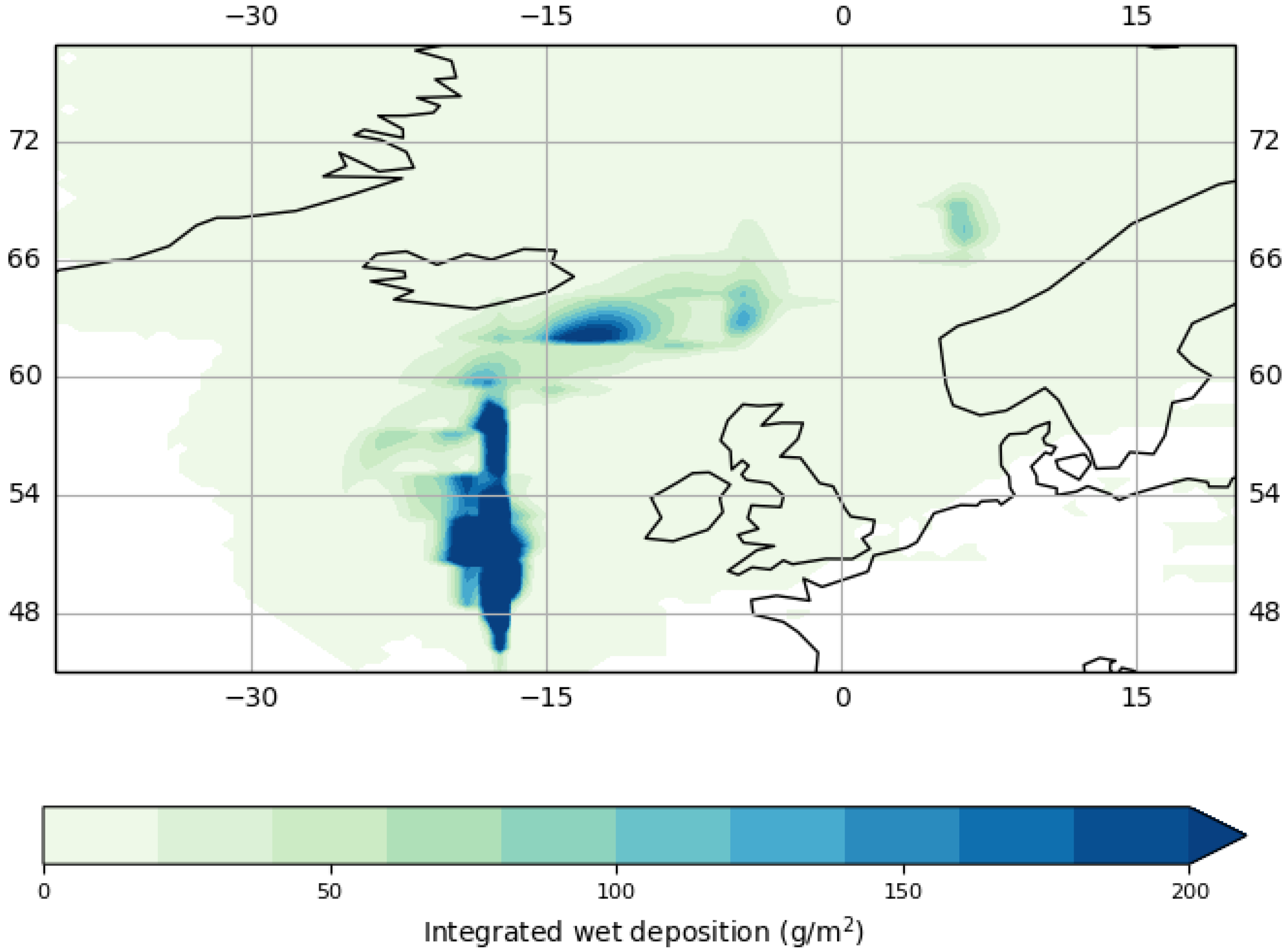
4.2. Quantifying Wet Deposition Uncertainty

As stated in Section 3, during the eruption there were several extratropical cyclones that transited the North Atlantic (as shown in Figure 2) which could impact ash location forecasts through small forecast errors in the NWP wind and precipitation location. The location of precipitation and meteorological cloud is important as ash is removed from the atmosphere by wet deposition [72]. Figure 7 shows the ensemble mean posterior wet deposition integrated over the duration of the Grímsvötn eruption (21–25 May 2011) from NAME simulations driven by the EPS meteorological ensemble. Wet deposition occurs over a large area with the largest values to the south and south-east of Iceland. The removal of ash by precipitation impacts atmospheric ash concentrations as less ash remains to be transported. To investigate the relative importance of potential wind and precipitation uncertainty, the InTEM inversion system was run again with the EPS meteorological ensemble but using NAME simulations without wet deposition processes being represented. This removes differences in the inversion that occur due to differences in the location and magnitude of forecast precipitation.
The ensemble of posterior emission profiles from InTEM without wet deposition represented are qualitatively similar to those shown in Figure 4 but with smaller emission rates. This is expected as, to match to the SEVIRI observations, less ash needs to be released if ash is not removed through wet deposition in the NAME simulations. The ensemble mean emission profile without wet deposition represented is shown in Figure 5. Please note that no ash was emitted for 15 h on 23 May for all members of the meteorological ensemble. Figure 6 shows the total emission rates over the whole eruption period for the posterior emissions with wet deposition processes represented (red circles show the mean, with the uncertainty (±one standard deviation) indicated by an orange bar) and without wet deposition processes represented (purple stars show the mean, with the uncertainty (±one standard deviation) indicated by lilac bars) for each ensemble member. The range of mean values for the ensemble without wet deposition is 0.81–0.97 × 10 12 g which is over a factor of 2 less than the range of total emissions for the ensemble with wet deposition processes represented (1.72–2.66 × 10 12 g). This suggests that in this case, wet deposition has a significant impact on the posterior emission rates. In both sets of inversions, the uncertainty of solutions for the total emission is large and skewed (yellow and pink bars in Figure 6) due to the non-negative constraint.
The ensemble mean total emission and standard deviation of the mean is shown in the last column of Figure 6. The ensemble mean total emission for the posterior emissions with wet deposition represented is 2.08 × 10 12 g with a standard deviation of 0.28 × 10 12 g compared to 0.89 × 10 12 g with a standard deviation of 0.04 × 10 12 g for the posterior emissions without wet deposition processes. The large separation of the ensemble means shows that the impact of wet deposition processes in the uncertainty on the total ash emitted is greater than uncertainty from the variability in the winds for this eruption.

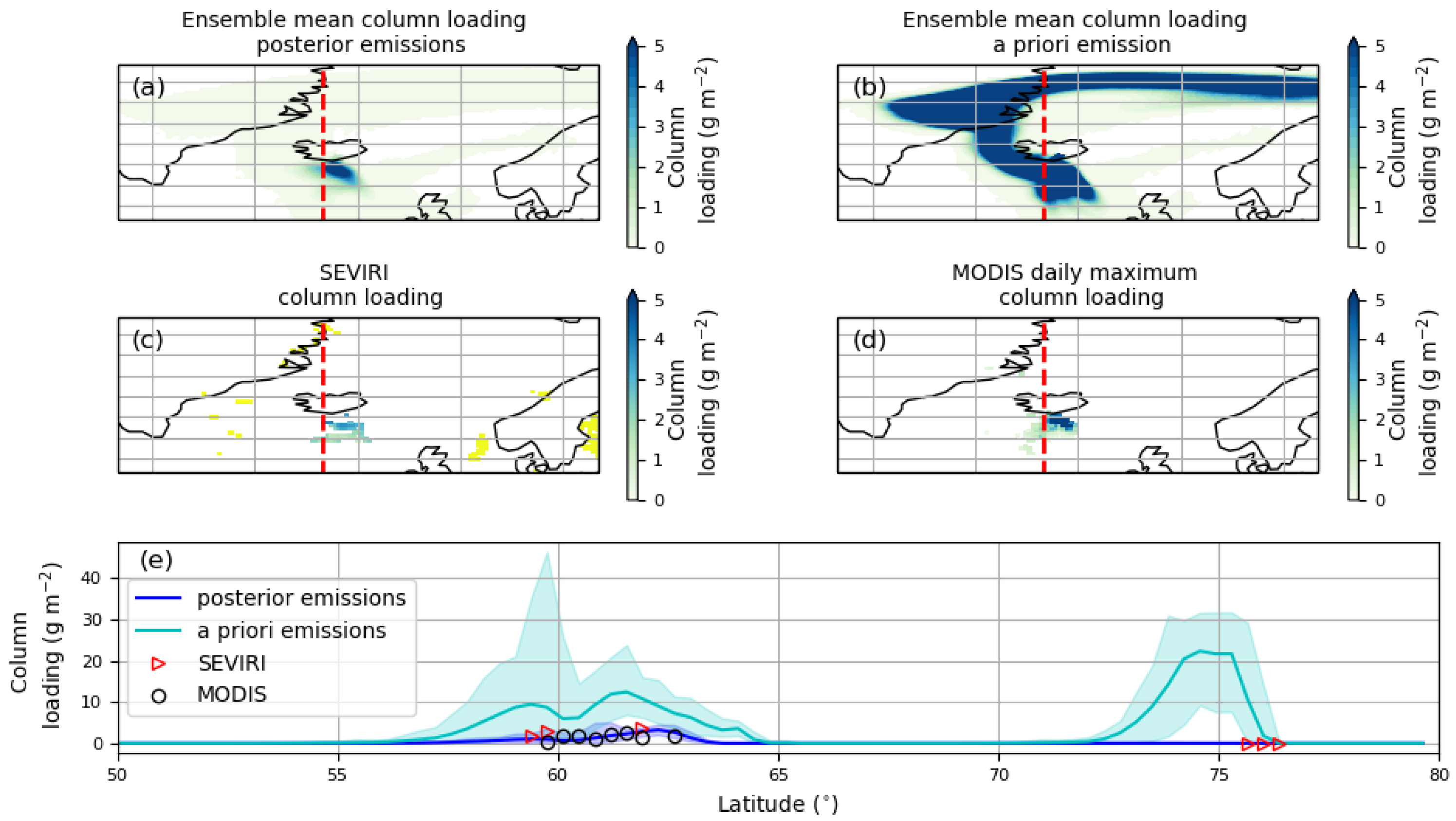
4.3. Ensemble InTEM Ash Forecasts

The previous discussion in Section 4.1 and Section 4.2 focused on the differences in posterior emission profiles; however VATD model forecasts of the ash cloud are used to inform VAAC graphics and advisories. This section analyses NAME simulations driven with the EPS meteorological ensemble both using the peak of the posterior distribution of emissions (shown in Figure 4) and a priori emissions and evaluates these simulations against independent satellite retrievals of volcanic ash from MODIS. Please note that the results presented use satellite retrievals for the whole eruption period (21–25 May 2011) and not just those retrievals available before 1800 UTC 23 May 2011 (Figure 8) and 0000 UTC 25 May 2011 (Figure 9).
Figure 8a,b show the spatial extent of the ash cloud at 1800 UTC 23 May 2011 for the ensemble of VATD model simulations with posterior emissions with wet deposition considered (Figure 8a) and a priori emissions (Figure 8b), while Figure 8c,d show SEVIRI (Figure 8c) and MODIS (Figure 8d) satellite retrievals. To ensure a fair comparison, these are presented as ensemble mean column loading but note that the VATD model simulations here use the default NAME particle size distribution which represents a range of particle sizes (0.1–100 μ m). Please note that the difference between this particle size distribution and what is found using by the satellite retrieval may contribute to discrepancies between the simulated and retrieved ash column loadings.
There is a large difference between the magnitude of the simulated ash clouds in Figure 8a,b. The ash cloud shown in Figure 8a is the mean of the simulations with posterior emissions. It extends south-east from the volcano with the maximum column loading values (greater than 4 g m 2 ) located to the south of Grímsvötn. This is quantitatively similar to both the SEVIRI retrievals used in the inversion process (Figure 8c) and the independent MODIS retrievals (Figure 8d). The mean ash cloud extent from the a priori ensemble has a much larger extent when considering column loadings greater than 4 g m 2 , both to the south-west and to the north-west with a filament extending from Greenland towards northern Scandinavia. As expected, this is very similar to the VAAC issued graphic shown in Figure 3. The region of highest column loading, 44.5 g m 2 , is over Greenland which is also consistent with the VAAC graphic (Figure 3). The region of highest mean column loading in the simulations with posterior emissions is located to the south-east of Grímsvötn with a magnitude of 7.8 g m 2 .
Figure 9a,b show a similar difference between the simulated ash clouds at 0000 UTC on 25 May 2011. This is 30 h later than the ash cloud shown in Figure 8 and before the end of the eruption at 0240 UTC on 25 May. The ash cloud from the a priori simulations is the most similar to the VAAC issued graphic (Figure 3b). On this day, MODIS did not detect any ash and there are a small number of SEVIRI pixels classified as ash over Scandinavia and clear sky pixels over Greenland and between the UK and mainland Europe. There may have been ash present at other locations at this time that could not be detected due to the presence of meteorological cloud.
Producing an ensemble of VATD simulations allows assessment of the ensemble spread. Figure 8e shows the range of posterior column loading values for the 20 posterior emission simulations (blue line and shading) and 20 a priori ensemble simulations (cyan line and shading) along the cross section shown in panels (a–d) as a red dashed line. The shading represents the uncertainty in ash column loading due to the meteorological ensemble. Satellite retrievals of ash column loading from SEVIRI (red triangles) and MODIS (black circles) are shown for comparison. Between 55–65 degrees north, the posterior ensemble spread encompasses both the MODIS and SEVIRI retrievals. The a priori ensemble has a much higher mean magnitude than the posterior emissions (by up to 200%) and the ensemble spread does not encompass the satellite observations. At 75 degrees north the a priori ensemble has a mean column loading of 21 g m 2 . However, the posterior emission ensemble predicts a very small amount of ash in this location which better matches the location of SEVIRI clear sky grid boxes at this time. Meteorological cloud obscures much of the domain so obtaining a contiguous retrieval of ashy and clear sky pixels is not possible at this time.
Figure 9e shows the same variables as Figure 8 at 0000 UTC 25 May 2011 along the cross section highlighted in panels (a–d) as a red dashed line. At this time there is no satellite retrieved ash along the cross section but there is a large number of SEVIRI grid boxes that are classified as clear sky (yellow shading). The magnitude of the column loading in the VATD simulations is approximately 10% of the column loadings shown in Figure 8. Along the cross section the mean column loading in the posterior emission ensemble is very small which agrees better with the location of SEVIRI clear sky observations. However, the a priori ensemble predicts ash between 65–75 N, with a large spread in forecast ash column loadings. This spread shows the variability that can be introduced by using an ensemble of meteorological conditions with the same ash emission profile.

5. Application of Probabilistic Volcanic Ash Forecasts for Flight Planning

During an eruption, aviation operators need to make fast and robust decisions concerning which flights to operate and whether flights already in the air need to be diverted. Presenting decision makers with graphics from a 20 member VATD forecast ensemble can be overwhelming and how they interpret the spread in the ensemble relies on the user’s risk appetite and experience [17].
Prata et al. [10] present a new method for visualizing ash concentration along flight paths using a risk-matrix approach. This risk approach is used by the UK Met Office when presenting forecasts of severe weather to the general public [73]. The methodology presented by Prata et al., determines the fraction of ensemble members that result in VATD model predicted concentrations over 3 different thresholds at three flight levels (surface-FL200, FL200-FL350 and FL350-FL550). The concentration thresholds used are 200–2000 μ g m 3 , 2000–4000 μ g m 3 and > 4000 μ g m 3 . The risk of encountering ash is the likelihood (or probability of exceedance) multiplied by impact (where the concentration ranges above are deemed to be low, medium and high impact respectively). In Prata et al. [10] the risk of flying in specific locations is then assigned to be low, medium or high.
The overall risk presented is the maximum risk over the three flight levels. This is a conservative estimate but consistent with current UK regulations that state that where possible, aircraft should laterally avoid forecasted areas of ash rather than over- or under-fly [7]. Please note that ICAO guidelines state that, for the purposes of flight planning, operators should treat the horizontal and vertical limits of the Danger Area to be overflown as it would mountainous terrain [3]. Prata et al. [10] suggest possible actions for the user for each of the risk levels, although these are a subset of the actions a flight planner might take. These range from checking updated forecasts, to loading more fuel and performing engine checks and considering other routes. The risk-matrix graphics reduce the state-of-the-art ensemble information into an easy to use decision making tool that can be used to make fast and scientifically robust decisions.
Figure 10 shows the risk determined using the Prata et al. [10] approach using both the posterior emissions ensemble with wet deposition considered and the a priori ensemble at 1800 UTC 23 May 2011 and 0000 UTC 25 May 2011. These ensembles represent the uncertainty in ash location and magnitude due to uncertainty in the meteorological situation. At both times, the region of forecasted risk is greatly reduced when the posterior emission ensemble is used compared to the a priori ensemble. At 1800 UTC 23 May, the forecasted risk area is reduced by 72%, with the highest risk area (blue) reduced by 88%. Similarly, at 0000 UTC 25 May, the forecasted risk area is reduced by 74%, with the highest risk area reduced by 97%. The area of forecasted risk determined by the a priori ensemble has a large extent to the north of Iceland with a further branch extending over the north of the UK into Scandinavia (Figure 10d). The posterior risk, also has a branch that extends from Iceland into Scandinavia (Figure 10b), although the risk diagnosed in this extension towards Europe is mostly at the medium level (turquoise). Please note that when calculating the likelihood of exceeding concentration thresholds, only uncertainty arising from the meteorology is estimated in this study.
At both times shown in Figure 10, if this risk-matrix approach is taken, for this eruption the disruption to airline operations has the potential to be greatly reduced if the posterior emissions were used. Please note that to be consistent with [10], the ash concentration fields output by NAME were multiplied by a factor of 10, known as the “peak-to-mean” factor. This factor accounts for peak concentrations that are not resolved by the NAME modeling [74]. This is similar to the operational approach of the London VAAC at the time of the Grímsvötn eruption, although the peak-to-mean-ratio is no longer applied operationally [16].

6. Summary and Conclusions

In the event of an emergency, aviation authorities need to make fast and robust decisions. These decisions take into account the VAAC forecasts which are informed by deterministic VATD model simulations. Two important inputs to these simulations are the ash emission source description and the driving NWP meteorological forecast. The determination of ash emissions in real time is, however, difficult. This study combines optimally estimated ash emission profiles using state-of-the-art inversion techniques with an ensemble of meteorological forecasts for the 2011 eruption of the Icelandic volcano Grímsvötn. Also determined is the dependence of emission estimates on wind and precipitation field uncertainty.
For this case study, the InTEM posterior ash emission rates are substantially reduced compared to the a priori emission profile that would be used if an inversion were not performed. The ensemble of posterior emission profiles, produced using a range of plausible meteorological situations, are similar but there are differences in the magnitude of the ash emitted at different heights. This leads to a large range of values (1.72–2.66 × 10 12 g) for the total amount of ash (in the size range 0.1–100 μ m) emitted over the eruption period. In the case study presented here, the inclusion of wet deposition processes, and the variability in the cloud and precipitation fields, has a greater impact on the uncertainty in the total amount of ash emitted than the variability of the winds. Despite the differences that are dominated by wet deposition uncertainty, the ensemble inversion provides confidence that the reduction of the a priori emissions, particularly above 4 km, is robust across all members. That is because, in this case, the emission profile and changing wind direction with height dominate this aspect of the simulations. The VATD model forecasts using the posterior emission ensemble have ash clouds with much lower column loadings compared to the a priori ensemble simulations. The posterior emission ensemble ash clouds are also a better match to the independent MODIS satellite retrievals of ash and have a much smaller range of column loadings.
The risk-matrix methodology outlined in Prata et al. [10] has been applied to the ensemble of forecast ash clouds obtained using the a priori and posterior emissions. In this case study, the use of the posterior emissions reduces the region of highest forecast risk by up to 94%. This could have large implications in emergency response situations and potentially reduce disruption to the civil flight plans.
The methodology presented in this paper focuses on the impact of meteorological uncertainty on the forecasting of volcanic ash location and concentration. There are many other sources of uncertainty that can contribute to uncertainty in ash forecasts which are not included here, such as uncertainties in the source (e.g., ash density) and uncertainties in the VATD model, for example, the representation of free tropospheric turbulence and unresolved mesoscale motions and the representation of wet deposition, that would ideally be included in an operational approach (as in [10]).
To be able to use an ensemble inversion approach in an emergency response situation, the ensemble of posterior emission profiles and associated forecast ash clouds need to be produced in a timely manner. The ensemble method is well suited to parallelization with different ensemble members run simultaneously on different cores. The current operational implementation of InTEM uses an iterative procedure whereby the posterior emissions can be updated during an ongoing eruption as more observations become available and the eruption progresses. Further work is needed to determine how the ensemble members should be combined to produce the best possible ash forecasts in this iterative framework.

7. Data Statement

The SEVIRI satellite data, NAME simulation and InTEM output are available in the University of Reading Research Data Archive at http://dx.doi.org/10.17864/1947.260. Further information about the data supporting these findings and requests for access to the data can be directed to [email protected]. The Oxford IASI volcanic products can be obtained by contacting Isabelle Taylor ([email protected]). For InTEM and NAME license enquiries, please contact the Met Office ([email protected]).

Author Contributions

Conceptualization, N.J.H. and H.F.D.; methodology, N.J.H. and H.F.D.; software, N.J.H. and H.N.W.; validation, N.J.H., investigation, N.J.H.; resources, N.J.H., S.K., M.C.C. and I.A.T.; writing—original draft preparation, N.J.H.; writing—review and editing, N.J.H., H.F.D., H.N.W., I.A.T. and R.G.G.; visualization, N.J.H. and I.A.T.; funding acquisition, H.F.D. and R.G.G. All authors have read and agreed to the published version of the manuscript.

Funding

N.J.H., H.F.D., H.N.W. are funded by the Natural Environment research council (NERC) grant number NE/S005218/1. I.A.T., R.G.G. and S.K. acknowledge NERC funding from R4Ash (NE/S003843/1) and V-PLUS (NE/S004025/1). I.A.T. and R.G.G. also acknowledge the support of the Center for Observation and Modeling of Earthquakes, Volcanoes and Tectonics.

Acknowledgments

We would like to acknowledge EUMETSAT and CEDA for access to the IASI level 1c spectra [75], and ECMWF and CEDA for the meteorological profiles used within the IASI retrievals [76]). We thank Keith Bevan (Lancaster University), and David Thomson (UK Met Office) for useful discussions on the methodology and Matt Hort (UK Met Office) for feedback on the manuscript.

Conflicts of Interest

The authors declare no conflict of interest. The funders had no role in the design of the study; in the collection, analyses, or interpretation of data; in the writing of the manuscript, or in the decision to publish the results.

References

  1. Casadevall, T.J. The 1989–1990 eruption of Redoubt Volcano, Alaska: Impacts on aircraft operations. J. Volcanol. Geotherm. Res. 1994, 62, 301–316. [Google Scholar] [CrossRef]
  2. Mazzocchi, M.; Hansstein, F.; Ragona, M. The volcanic ash cloud and its financial impact on the European airline industry. In CESifo Forum; No 2:92-100; Ifo Institut für Wirtschaftsforschung an der Universität München: München, Germany, 2010. [Google Scholar]
  3. Doc 9691 AN/954: Manual on Volcanic Ash, Radioactive Material and Toxic Chemical Clouds, 2nd ed.; International Civil Aviation Organization: Montréal, QC, Canada, 2007; Available online: https://skybrary.aero/bookshelf/books/2997.pdf (accessed on 5 February 2020).
  4. Witham, C.; Webster, H.; Hort, M.; Jones, A.; Thomson, D. Modelling concentrations of volcanic ash encountered by aircraft in past eruptions. Atmos. Environ. 2012, 48, 219–229. [Google Scholar] [CrossRef]
  5. Clarkson, R.J.; Majewicz, E.J.; Mack, P. A re-evaluation of the 2010 quantitative understanding of the effects volcanic ash has on gas turbine engines. Proc. Inst. Mech. Eng. Part G J. Aerosp. Eng. 2016, 230, 2274–2291. [Google Scholar] [CrossRef]
  6. European Commission. Volcano Grimsvötn: How Is the European Response Different to the Eyjafjallajökull Eruption Last Year? Frequently Asked Questions; European Commission: Brussels, Belgium, 2011. [Google Scholar]
  7. UK Civil Aviation Authority. CAP1236: Guidance Regarding Flight Operations in the Vicinity of Volcanic Ash; UK Civil Aviation Authority: London, UK, 2017. [Google Scholar]
  8. Dacre, H.; Grant, A.; Hogan, R.; Belcher, S.; Thomson, D.; Devenish, B.; Marenco, F.; Hort, M.; Haywood, J.M.; Ansmann, A.; et al. Evaluating the structure and magnitude of the ash plume during the initial phase of the 2010 Eyjafjallajökull eruption using lidar observations and NAME simulations. J. Geophys. Res. 2011, 116. [Google Scholar] [CrossRef]
  9. Harvey, N.J.; Huntley, N.; Dacre, H.F.; Goldstein, M.; Thomson, D.; Webster, H. Multi-level emulation of a volcanic ash transport and dispersion model to quantify sensitivity to uncertain parameters. Nat. Hazards Earth Syst. Sci. 2018, 18, 41–63. [Google Scholar] [CrossRef] [Green Version]
  10. Prata, A.T.; Dacre, H.F.; Irvine, E.A.; Mathieu, E.; Shine, K.P.; Clarkson, R.J. Calculating and communicating ensemble-based volcanic ash dosage and concentration risk for aviation. Meteorol. Appl. 2019, 26, 253–266. [Google Scholar] [CrossRef] [Green Version]
  11. Petersen, G.N.; Bjornsson, H.; Arason, P.; von Löwis, S. Two weather radar time series of the altitude of the volcanic plume during the May 2011 eruption of Grimsvotn, Iceland. Earth Syst. Sci. Data 2012, 4, 121–127. [Google Scholar] [CrossRef] [Green Version]
  12. Mastin, L.; Guffanti, M.; Servranckx, R.; Webley, P.; Barsotti, S.; Dean, K.; Durant, A.; Ewert, J.; Neri, A.; Rose, W.; et al. A multidisciplinary effort to assign realistic source parameters to models of volcanic ash-cloud transport and dispersion during eruptions. J. Volcanol. Geotherm. Res. 2009, 186, 10–21. [Google Scholar] [CrossRef]
  13. Sparks, R.S.J.; Bursik, M.; Carey, S.; Gilbert, J.; Glaze, L.; Sigurdsson, H.; Woods, A. Volcanic Plumes; Wiley: Chichester, UK, 1997. [Google Scholar]
  14. Woodhouse, M.J.; Hogg, A.J.; Phillips, J.C.; Sparks, R.S.J. Interaction between volcanic plumes and wind during the 2010 Eyjafjallajökull eruption, Iceland. J. Geophys. Res. 2013, 118, 92–109. [Google Scholar] [CrossRef] [Green Version]
  15. Bonadonna, C.; Folch, A.; Loughlin, S.; Puempel, H. Future developments in modelling and monitoring of volcanic ash clouds: Outcomes from the first IAVCEI-WMO workshop on Ash Dispersal Forecast and Civil Aviation. Bull. Volcanol. 2012, 74, 1–10. [Google Scholar] [CrossRef] [Green Version]
  16. Beckett, F.M.; Witham, C.S.; Leadbetter, S.J.; Crocker, R.; Webster, H.N.; Hort, M.C.; Jones, A.R.; Devenish, B.J.; Thomson, D.J. Atmospheric Dispersion Modelling at the London VAAC: A Review of Developments since the 2010 Eyjafjallajökull Volcano Ash Cloud. Atmosphere 2020, 11, 352. [Google Scholar] [CrossRef] [Green Version]
  17. Mulder, K.J.; Lickiss, M.; Harvey, N.; Black, A.; Charlton-Perez, A.; Dacre, H.; McCloy, R. Visualizing Volcanic Ash Forecasts: Scientist and Stakeholder Decisions Using Different Graphical Representations and Conflicting Forecasts. Weather. Clim. Soc. 2017, 9, 333–348. [Google Scholar] [CrossRef] [Green Version]
  18. Dare, R.A.; Potts, R.J.; Wain, A.G. Modelling wet deposition in simulations of volcanic ash dispersion from hypothetical eruptions of Merapi, Indonesia. Atmos. Environ. 2016, 143, 190–201. [Google Scholar] [CrossRef]
  19. Zidikheri, M.J.; Lucas, C.; Potts, R.J. Quantitative verification and calibration of volcanic ash ensemble forecasts using satellite data. J. Geophys. Res. Atmos. 2018, 123, 4135–4156. [Google Scholar] [CrossRef]
  20. Stefanescu, E.; Patra, A.; Bursik, M.; Madankan, R.; Pouget, S.; Jones, M.; Singla, P.; Singh, T.; Pitman, E.; Pavolonis, M.; et al. Temporal, probabilistic mapping of ash clouds using wind field stochastic variability and uncertain eruption source parameters: Example of the 14 April 2010 Eyjafjallajökull eruption. J. Adv. Model. Earth Syst. 2014, 6, 1173–1184. [Google Scholar] [CrossRef] [Green Version]
  21. Madankan, R.; Pouget, S.; Singla, P.; Bursik, M.; Dehn, J.; Jones, M.; Patra, A.; Pavolonis, M.; Pitman, E.B.; Singh, T.; et al. Computation of probabilistic hazard maps and source parameter estimation for volcanic ash transport and dispersion. J. Comput. Phys. 2014, 271, 39–59. [Google Scholar] [CrossRef]
  22. Dacre, H.F.; Harvey, N.J. Characterizing the Atmospheric Conditions Leading to Large Error Growth in Volcanic Ash Cloud Forecasts. J. Appl. Meteorol. Climatol. 2018, 57, 1011–1019. [Google Scholar] [CrossRef]
  23. Langmann, B.; Zakšek, K.; Hort, M. Atmospheric distribution and removal of volcanic ash after the eruption of Kasatochi volcano: A regional model study. J. Geophys. Res. Atmos. 2010, 115. [Google Scholar] [CrossRef]
  24. Francis, P.N.; Cooke, M.C.; Saunders, R.W. Retrieval of physical properties of volcanic ash using Meteosat: A case study from the 2010 Eyjafjallajökull eruption. J. Geophys. Res. 2012, 117. [Google Scholar] [CrossRef]
  25. Pavolonis, M.J.; Heidinger, A.K.; Sieglaff, J. Automated retrievals of volcanic ash and dust cloud properties from upwelling infrared measurements. J. Geophys. Res. Atmos. 2013, 118, 1436–1458. [Google Scholar] [CrossRef]
  26. Kristiansen, N.I.; Stohl, A.; Prata, A.J.; Bukowiecki, N.; Dacre, H.; Eckhardt, S.; Henne, S.; Hort, M.C.; Johnson, B.T.; Marenco, F.; et al. Performance assessment of a volcanic ash transport model mini-ensemble used for inverse modeling of the 2010 Eyjafjallajökull eruption. J. Geophys. Res. 2012, 117. [Google Scholar] [CrossRef] [Green Version]
  27. Schmehl, K.J.; Haupt, S.E.; Pavolonis, M.J. A genetic algorithm variational approach to data assimilation and application to volcanic emissions. Pure Appl. Geophys. 2012, 169, 519–537. [Google Scholar] [CrossRef]
  28. Denlinger, R.P.; Pavolonis, M.; Sieglaff, J. A robust method to forecast volcanic ash clouds. J. Geophys. Res. 2012, 117. [Google Scholar] [CrossRef]
  29. Pelley, R.E.; Cooke, M.C.; Manning, A.J.; Thomson, D.J.; Witham, C.S.; Hort, M.C. Initial Implementation of an Inversion Techniques for Estimating Volcanic Ash Source Parameters in Near Real Time Using Satellite Retrievals; Forecasting Research Technical Report No. 644; Met Office: Exeter, UK, 2015. [Google Scholar]
  30. Zidikheri, M.J.; Lucas, C.; Potts, R.J. Toward quantitative forecasts of volcanic ash dispersal: Using satellite retrievals for optimal estimation of source terms. J. Geophys. Res. Atmos. 2017, 122, 8187–8206. [Google Scholar] [CrossRef]
  31. Zidikheri, M.J.; Lucas, C.; Potts, R.J. Estimation of optimal dispersion model source parameters using satellite detections of volcanic ash. J. Geophys. Res. Atmos. 2017, 122, 8207–8232. [Google Scholar] [CrossRef]
  32. Eckhardt, S.; Prata, A.; Seibert, P.; Stebel, K.; Stohl, A. Estimation of the vertical profile of sulfur dioxide injection into the atmosphere by a volcanic eruption using satellite column measurements and inverse transport modeling. Atmos. Chem. Phys. 2008, 8, 3881–3897. [Google Scholar] [CrossRef] [Green Version]
  33. Kristiansen, N.; Stohl, A.; Prata, A.; Richter, A.; Eckhardt, S.; Seibert, P.; Hoffmann, A.; Ritter, C.; Bitar, L.; Duck, T.; et al. Remote sensing and inverse transport modeling of the Kasatochi eruption sulfur dioxide cloud. J. Geophys. Res. Atmos. 2010, 115. [Google Scholar] [CrossRef]
  34. Stohl, A.; Prata, A.; Eckhardt, S.; Clarisse, L.; Durant, A.; Henne, S.; Kristiansen, N.; Minikin, A.; Schumann, U.; Seibert, P.; et al. Determination of time-and height-resolved volcanic ash emissions and their use for quantitative ash dispersion modeling: The 2010 Eyjafjallajökull eruption. Atmos. Chem. Phys. 2011, 11, 4333–4351. [Google Scholar] [CrossRef] [Green Version]
  35. Seibert, P.; Kristiansen, N.I.; Richter, A.; Eckhardt, S.; Prata, A.J.; Stohl, A. Uncertainties in the inverse modelling of sulphur dioxide eruption profiles. Geomat. Nat. Hazards Risk 2011, 2, 201–216. [Google Scholar] [CrossRef]
  36. Boichu, M.; Menut, L.; Khvorostyanov, D.; Clarisse, L.; Clerbaux, C.; Turquety, S.; Coheur, P.F. Inverting for volcanic SO2 flux at high temporal resolution using spaceborne plume imagery and chemistry-transport modelling: The 2010 Eyjafjallajökull eruption case-study. Atmos. Chem. Phys. 2013, 13, 8569–8584. [Google Scholar] [CrossRef] [Green Version]
  37. Zidikheri, M.J.; Potts, R.J. A simple inversion method for determining optimal dispersion model parameters from satellite detections of volcanic sulfur dioxide. J. Geophys. Res. Atmos. 2015, 120, 9702–9717. [Google Scholar] [CrossRef]
  38. Moxnes, E.; Kristiansen, N.; Stohl, A.; Clarisse, L.; Durant, A.; Weber, K.; Vogel, A. Separation of ash and sulfur dioxide during the 2011 Grímsvötn eruption. J. Geophys. Res. Atmos. 2014, 119, 7477–7501. [Google Scholar] [CrossRef] [Green Version]
  39. Zidikheri, M.J.; Lucas, C. Using Satellite Data to Determine Empirical Relationships between Volcanic Ash Source Parameters. Atmosphere 2020, 11, 342. [Google Scholar] [CrossRef] [Green Version]
  40. Molteni, F.; Buizza, R.; Palmer, T.N.; Petroliagis, T. The ECMWF Ensemble Prediction System: Methodology and validation. Q. J. R. Meteorol. Soc. 1996, 122, 73–119. [Google Scholar] [CrossRef]
  41. Buizza, R.; Palmer, T.N. The singular-vector structure of the atmospheric global circulation. J. Atmos. Sci. 1995, 52, 1434–1456. [Google Scholar] [CrossRef] [Green Version]
  42. Buizza, R.; Milleer, M.; Palmer, T.N. Stochastic representation of model uncertainties in the ECMWF ensemble prediction system. Q. J. R. Meteorol. Soc. 1999, 125, 2887–2908. [Google Scholar] [CrossRef]
  43. Thomson, D.J.; Webster, H.N.; Cooke, M.C. Developments in the Met Office InTEM Volcanic Ash Source Estimation System Part 1: Concepts; Met Office: Exeter, UK, 2017. [Google Scholar]
  44. Clerbaux, C.; Boynard, A.; Clarisse, L.; George, M.; Hadji-Lazaro, J.; Herbin, H.; Hurtmans, D.; Pommier, M.; Razavi, A.; Turquety, S.; et al. Monitoring of atmospheric composition using the thermal infrared IASI/MetOp sounder. Atmos. Chem. Phys. 2009, 9, 6041–6054. [Google Scholar] [CrossRef] [Green Version]
  45. Theys, N.; Campion, R.; Clarisse, L.; Brenot, H.; van Gent, J.; Dils, B.; Corradini, S.; Merucci, L.; Coheur, P.F.; Van Roozendael, M.; et al. Volcanic SO2 fluxes derived from satellite data: A survey using OMI, GOME-2, IASI and MODIS. Atmos. Chem. Phys. 2013, 13, 5945–5968. [Google Scholar] [CrossRef] [Green Version]
  46. Clarisse, L.; Prata, F.; Lacour, J.L.; Hurtmans, D.; Clerbaux, C.; Coheur, P.F. A correlation method for volcanic ash detection using hyperspectral infrared measurements. Geophys. Res. Lett. 2010, 37. [Google Scholar] [CrossRef] [Green Version]
  47. Clarisse, L.; Coheur, P.F.; Prata, A.; Hurtmans, D.; Razavi, A.; Phulpin, T.; Hadji-Lazaro, J.; Clerbaux, C. Tracking and quantifying volcanic SO2 with IASI, the September 2007 eruption at Jebel at Tair. Atmos. Chem. Phys. 2008, 8, 7723–7734. [Google Scholar] [CrossRef] [Green Version]
  48. Clarisse, L.; Hurtmans, D.; Prata, A.J.; Karagulian, F.; Clerbaux, C.; Mazière, M.D.; Coheur, P.F. Retrieving radius, concentration, optical depth, and mass of different types of aerosols from high-resolution infrared nadir spectra. Appl. Opt. 2010, 49, 3713–3722. [Google Scholar] [CrossRef] [PubMed]
  49. Clarisse, L.; Hurtmans, D.; Clerbaux, C.; Hadji-Lazaro, J.; Ngadi, Y.; Coheur, P.F. Retrieval of sulphur dioxide from the infrared atmospheric sounding interferometer (IASI). Atmos. Meas. Tech. 2012, 5, 581–594. [Google Scholar] [CrossRef] [Green Version]
  50. Carboni, E.; Grainger, R.; Walker, J.; Dudhia, A.; Siddans, R. A new scheme for sulphur dioxide retrieval from IASI measurements: Application to the Eyjafjallajökull eruption of April and May 2010. Atmos. Chem. Phys. 2012, 12, 11417–11434. [Google Scholar] [CrossRef] [Green Version]
  51. Walker, J.C.; Carboni, E.; Dudhia, A.; Grainger, R.G. Improved detection of sulphur dioxide in volcanic plumes using satellite-based hyperspectral infrared measurements: Application to the Eyjafjallajökull 2010 eruption. J. Geophys. Res. Atmos. 2012, 117. [Google Scholar] [CrossRef] [Green Version]
  52. Ventress, L.J.; McGarragh, G.; Carboni, E.; Smith, A.J.; Grainger, R.G. Retrieval of ash properties from IASI measurements. Atmos. Meas. Tech. 2016, 9, 5407–5422. [Google Scholar] [CrossRef] [Green Version]
  53. Taylor, I.A.; Carboni, E.; Ventress, L.J.; Mather, T.A.; Grainger, R.G. An adaptation of the CO2 slicing technique for the Infrared Atmospheric Sounding Interferometer to obtain the height of tropospheric volcanic ash clouds. Atmos. Meas. Tech. 2019, 12, 3853–3883. [Google Scholar] [CrossRef] [Green Version]
  54. Reed, B.E.; Peters, D.M.; McPheat, R.; Grainger, R.G. The Complex Refractive Index of Volcanic Ash Aerosol Retrieved From Spectral Mass Extinction. J. Geophys. Res. Atmos. 2018, 123, 1339–1350. [Google Scholar] [CrossRef] [Green Version]
  55. Barnes, W.L.; Pagano, T.S.; Salomonson, V.V. Prelaunch characteristics of the Moderate Resolution Imaging Spectroradiometer (MODIS) on EOS-AM1. IEEE Trans. Geosci. Remote Sens. 1998, 36, 1088–1100. [Google Scholar] [CrossRef] [Green Version]
  56. MODIS Characterization Support Team (MCST). MODIS 1 km Calibrated Radiances Product; Goddard Space Flight Center: Greenbelt, MD, USA, 2017; Available online: http://dx.doi.org/10.5067/MODIS/MYD021KM.061 (accessed on 1 April 2020).
  57. Poulsen, C.; Siddans, R.; Thomas, G.; Sayer, A.; Grainger, R.; Campmany, E.; Dean, S.; Arnold, C.; Watts, P. Cloud retrievals from satellite data using optimal estimation: Evaluation and application to ATSR. Atmos. Meas. Tech. 2012, 5, 1889. [Google Scholar] [CrossRef] [Green Version]
  58. McGarragh, G.R.; Poulsen, C.A.; Thomas, G.E.; Povey, A.C.; Sus, O.; Stapelberg, S.; Schlundt, C.; Proud, S.; Christensen, M.W.; Stengel, M.; et al. The Community Cloud retrieval for CLimate (CC4CL)—Part 2: The optimal estimation approach. Atmos. Meas. Tech. 2018, 11, 3397–3431. [Google Scholar] [CrossRef] [Green Version]
  59. Jones, A.; Thomson, D.; Hort, M.; Devenish, B. The UK Met Office’s next-generation atmospheric dispersion model, NAME III. In Air Pollution Modeling and Its Application XVII; Springer: Boston, MA, USA, 2007; pp. 580–589. [Google Scholar]
  60. Hobbs, P.V.; Radke, L.F.; Lyons, J.H.; Ferek, R.J.; Coffman, D.J.; Casadevall, T.J. Airborne measurements of particle and gas emissions from the 1990 volcanic eruptions of Mount Redoubt. J. Geophys. Res. 1991, 96, 18735–18752. [Google Scholar] [CrossRef] [Green Version]
  61. Manning, A.J.; O’Doherty, S.; Jones, A.R.; Simmonds, P.G.; Derwent, R.G. Estimating UK methane and nitrous oxide emissions from 1990 to 2007 using an inversion modeling approach. J. Geophys. Res. Atmos. 2011, 116. [Google Scholar] [CrossRef]
  62. Lawson, C.L.; Hanson, R.J. Solving Least Squares Problems; Prentice-Hall: Englewood Cliffs, NJ, USA, 1974. [Google Scholar]
  63. Webster, H.N.; Thomson, D.J.; Cooke, M.C. Developments in the Met Office InTEM Volcanic Ash Source Estimation System Part 2: Results; Met Office: Exeter, UK, 2017. [Google Scholar]
  64. Prata, F.; Woodhouse, M.; Huppert, H.E.; Prata, A.; Thordarson, T.; Carn, S. Atmospheric processes affecting the separation of volcanic ash and SO2 in volcanic eruptions: Inferences from the May 2011 Grímsvötn eruption. Atmos. Chem. Phys. 2017, 17, 10709–10732. [Google Scholar] [CrossRef] [Green Version]
  65. Stevenson, J.A.; Loughlin, S.C.; Font, A.; Fuller, G.W.; MacLeod, A.; Oliver, I.W.; Jackson, B.; Horwell, C.J.; Thordarson, T.; Dawson, I. UK monitoring and deposition of tephra from the May 2011 eruption of Grímsvötn, Iceland. J. Appl. Volcanol. 2013, 2, 3. [Google Scholar] [CrossRef] [Green Version]
  66. Tesche, M.; Glantz, P.; Johansson, C.; Norman, M.; Hiebsch, A.; Ansmann, A.; Althausen, D.; Engelmann, R.; Seifert, P. Volcanic ash over Scandinavia originating from the Grímsvötn eruptions in May 2011. J. Geophys. Res. 2012, 117. [Google Scholar] [CrossRef]
  67. UK Met Office. London VAAC: Volcanic ash Advisories and Graphics Archive. 2020. Available online: https://www.metoffice.gov.uk/services/transport/aviation/regulated/vaac/advisories/archive (accessed on 1 April 2020).
  68. Cooke, M.C.; Francis, P.N.; Millington, S.; Saunders, R.; Witham, C. Detection of the Grímsvötn 2011 volcanic eruption plumes using infrared satellite measurements. Atmos. Sci. Lett. 2014, 15, 321–327. [Google Scholar] [CrossRef]
  69. Kerminen, V.M.; Niemi, J.; Timonen, H.; Aurela, M.; Frey, A.; Carbone, S.; Saarikoski, S.; Teinilä, K.; Hakkarainen, J.; Tamminen, J.; et al. Characterization of a volcanic ash episode in southern Finland caused by the Grimsvotn eruption in Iceland in May 2011. Atmos. Chem. Phys. 2011, 11, 12227. [Google Scholar] [CrossRef] [Green Version]
  70. Cazacu, M.; Timofte, A.; Talianu, C.; Nicolae, D.; Danila, M.; Unga, F.; Dimitriu, D.; Gurlui, S. Grímsvötn volcano: Atmospheric volcanic ash cloud investigations, modelling-forecast and experimental environmental approach upon the Romanian area. J. Optoelectron. Adv. Mater. 2012, 14, 517. [Google Scholar]
  71. Kvietkus, K.; Šakalys, J.; Didžbalis, J.; Garbarienė, I.; Špirkauskaitė, N.; Remeikis, V. Atmospheric aerosol episodes over Lithuania after the May 2011 volcano eruption at Grimsvötn, Iceland. Atmos. Res. 2013, 122, 93–101. [Google Scholar] [CrossRef]
  72. Pruppacher, H.R.; Klett, J.D. Microphysics of clouds and precipitation. Nature 1980, 284, 88. [Google Scholar] [CrossRef]
  73. Neal, R.A.; Boyle, P.; Grahame, N.; Mylne, K.; Sharpe, M. Ensemble based first guess support towards a risk-based severe weather warning service. Meteorol. Appl. 2014, 21, 563–577. [Google Scholar] [CrossRef]
  74. Webster, H.; Thomson, D.; Johnson, B.; Heard, I.; Turnbull, K.; Marenco, F.; Kristiansen, N.; Dorsey, J.; Minikin, A.; Weinzierl, B.; et al. Operational prediction of ash concentrations in the distal volcanic cloud from the 2010 Eyjafjallajökull eruption. J. Geophys. Res. 2012, 117. [Google Scholar] [CrossRef] [Green Version]
  75. EUMETSAT. IASI: Atmospheric Sounding Level 1C Data Products; NERC Earth Observation Data Centre: Oxford, UK, 2009. Available online: https://catalogue.ceda.ac.uk/uuid/ea46600afc4559827f31dbfbb8894c2e (accessed on 27 August 2020).
  76. European Centre for Medium-Range Weather Forecasts. ECMWF Operational Regular Gridded Data at 1.125 Degrees Resolution; NCAS British Atmospheric Data Centre: Oxford, UK, 2012; Available online: https://catalogue.ceda.ac.uk/uuid/a67f1b4d9db7b1528b800ed48198bdac (accessed on 27 August 2020).
Figure 1. (a) Maximum observed SO 2 column amount and (b) Maximum observed ash column loading for the period between 21 and 26 May 2011 inclusive. The IASI retrieval outputs were gridded for each orbit and, similar to Moxnes et al. (2014), the maximum value observed during all the overpasses in the given period is shown.
Atmosphere 11 01022 g001
Figure 2. UK Met Office surface analysis chart at 0000 UTC on 22 May 2011. Mean sea level pressure isobars overlaid with active surface fronts (solid black lines with filled symbols), decaying surface fronts (crosses with filled symbols) upper-level fronts (solid black lines with unfilled symbols) and upper-level troughs (solid black lines).
Atmosphere 11 01022 g002
Figure 3. Volcanic ash advisory graphics issued by the London VAAC at (a) 1800 UTC on 23 May 2011 and (b) 0000 UTC on 25 May 2011 taken from the London VAAC: Volcanic ash advisories and graphics archive [67]. Contours show the outermost extent of the ash cloud in 3 layers of the atmosphere: surface—flight level (FL) 200 (red), FL200-350 (green) and FL350-550 (blue).
Atmosphere 11 01022 g003
Figure 4. Posterior emission profiles (g/h) estimated by InTEM for the 2011 Grímsvötn eruption for each member of the ECMWF EPS ensemble using SEVIRI retrievals of ash and clear skies. Note the logarithmic color scale.
Atmosphere 11 01022 g004
Figure 5. (a) a priori (b) ensemble mean posterior with wet deposition represented (c) ensemble mean posterior without wet deposition represented time-height emission profile (g/h) determined by InTEM for the Grímsvötn eruption (21–25 May 2011). Note the log scale used for the release rate.
Atmosphere 11 01022 g005
Figure 6. Total ash emitted during the Grímsvötn eruption for each ensemble member in the EPS ensemble determined using InTEM. Red circles and orange bars indicate the peak in the posterior distribution and range (±one standard deviation) of the total ash emitted for simulations that include wet deposition. Purple stars and lilac bars indicate the peak of the posterior distribution and range of the total ash emitted for simulations that do not include wet deposition. The final column shows the mean and standard deviation for the ensemble emissions with (blue circle and cyan bar) and without wet deposition (green star and light green bar).
Atmosphere 11 01022 g006
Figure 7. Ensemble mean wet deposition integrated over the duration of the Grímsvötn eruption (21–25 May 2011).
Atmosphere 11 01022 g007
Figure 8. (a) Ensemble mean ash column loading at 1800 UTC 23 May 2011 for simulations run with emission profiles determined using InTEM with matching ensemble meteorology at 1800 UTC 23 May 2011, (b) Ensemble mean ash column loading at 1800 UTC 23 May 2011 for simulations run with a priori emission profile and ensemble meteorology, (c) SEVIRI ash column loading (yellow shading indicates grid boxes that are classified as clear sky) (d) Daily MODIS maximum ash column loading for 23 May 2011, (e) Ash column loading profile along the cross section indicated by the red dashed line in panels (ad) for the posterior ensemble (blue), a priori ensemble (cyan), SEVIRI ash column loading (red triangles) and MODIS ash column loading (black circles). The shading indicates the range of column loading in the ensemble.
Atmosphere 11 01022 g008
Figure 9. As Figure 8 for 0000 UTC on 25 May 2011. Note MODIS (panel d) did not retrieve any ash on this day.
Atmosphere 11 01022 g009
Figure 10. Overall ash concentration risk map at (a,c) 1800 UTC on 23 May 2011, (b,d) 0000 UTC on 25 May 2011 for (a,b) simulations with posterior emissions with matching ensemble meteorology and (c,d) simulations with a priori emissions with ensemble meteorology. Green shading indicates the lowest level of risk, turquoise shading indicates mid-level risk and purple indicates the highest level of risk.
Atmosphere 11 01022 g010

