Frontal Wind Field Retrieval Based on UHF Wind Profiler Radars and S-Band Radars Network


Abstract
1. Introduction
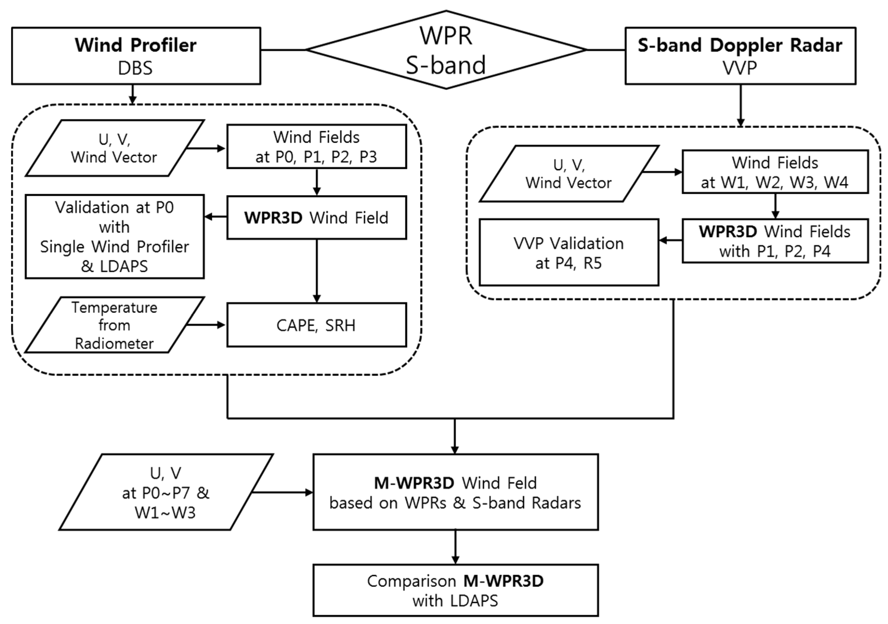
2. Data and Method
2.1. Data
2.2. Analysis Method
2.2.1. Three-Dimensional Wind Field Processing
2.2.2. Convective Instability Indices
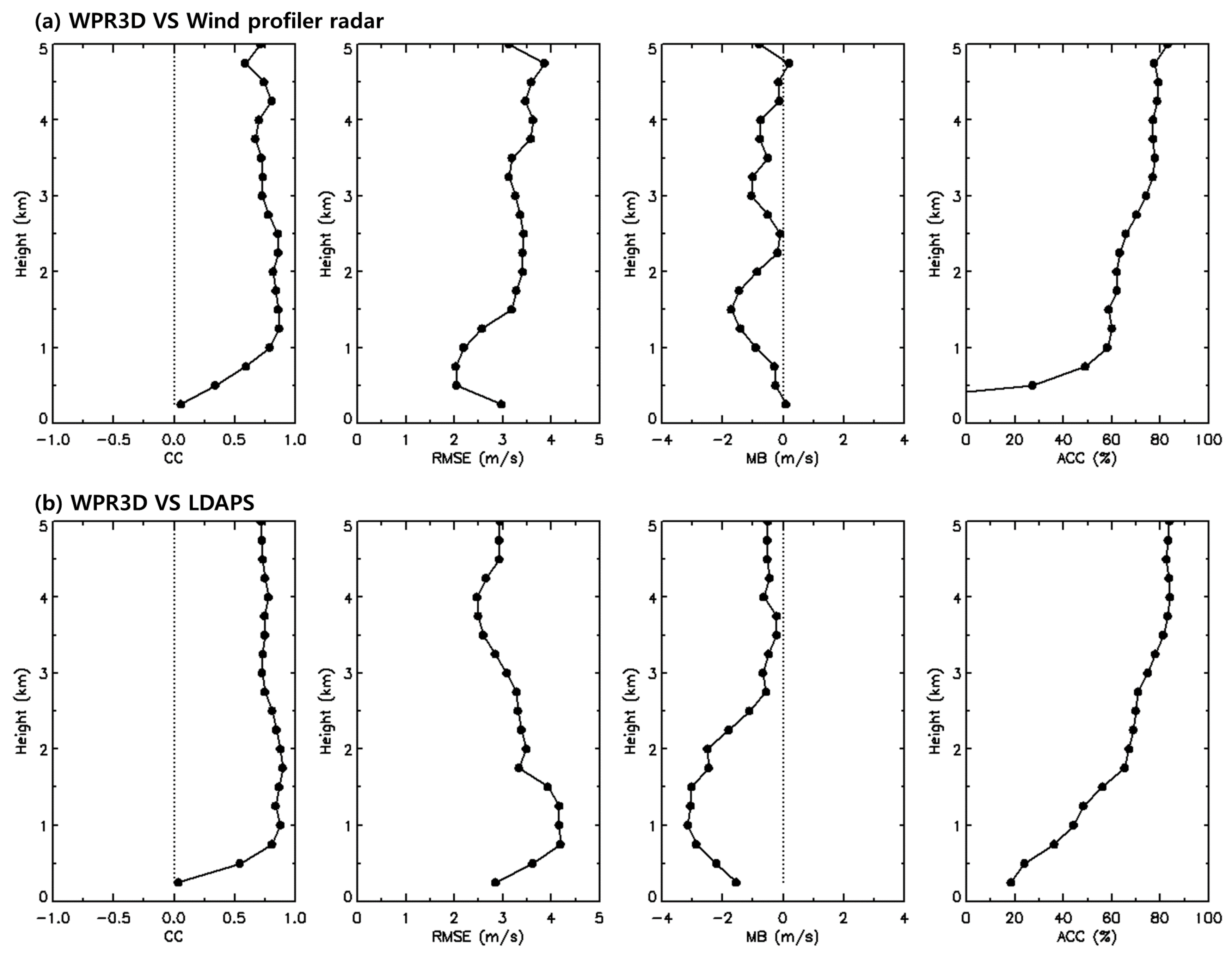
2.2.3. Accuracy Validation
3. Results and Discussion
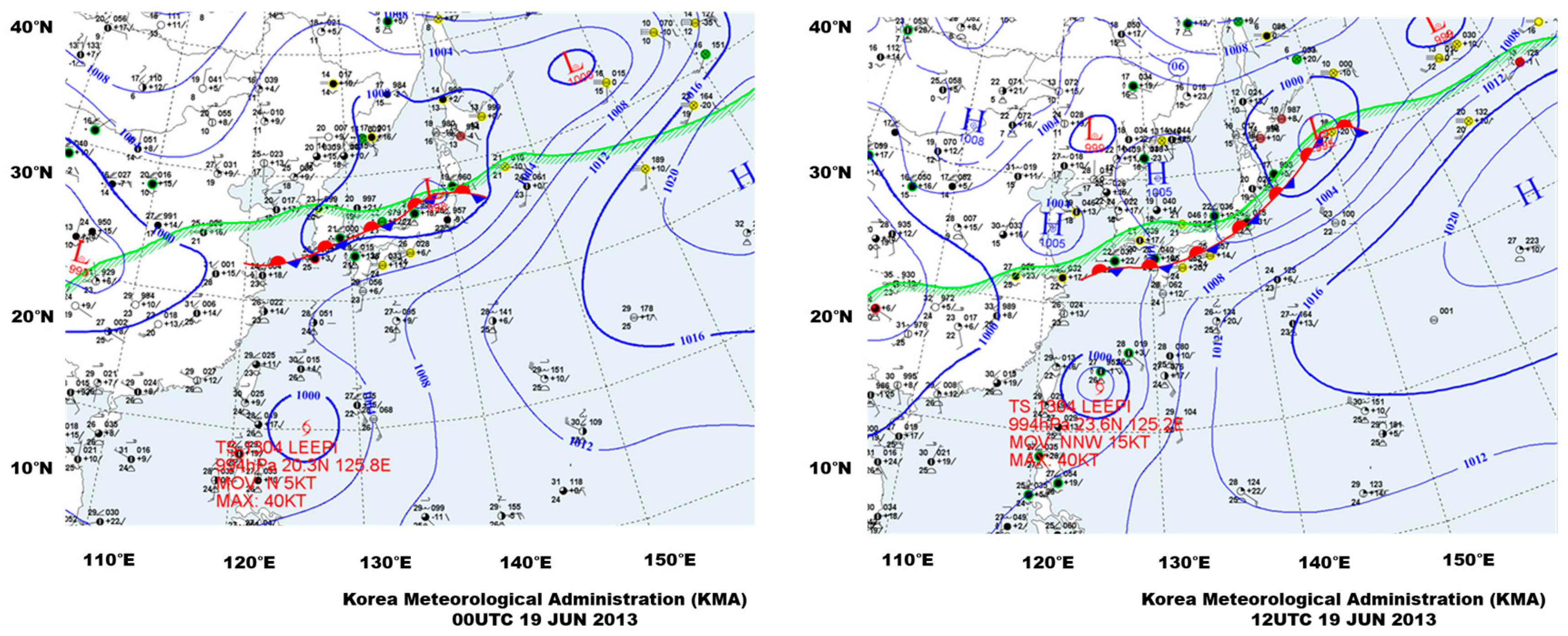
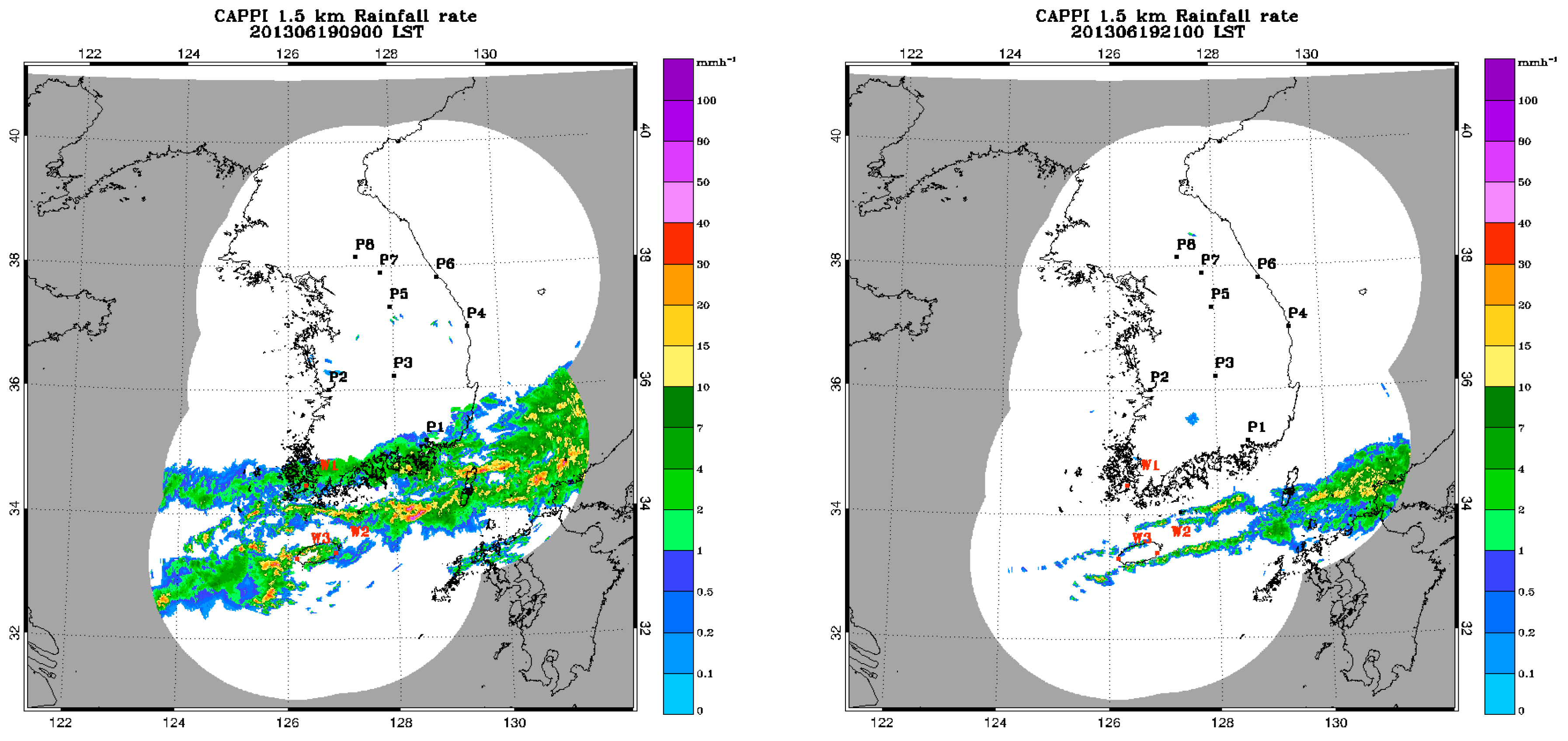
3.1. Synoptic Conditions and Frontal Structure
3.2. Assessment of Frontal Winds from a Single WPR3D
3.3. Instability and Wind Field
3.4. Multiple WPR3D Wind Field
4. Conclusions
Author Contributions
Funding
Acknowledgments
Conflicts of Interest
References
- Chen, T.-J.G.; Chang, C.-P. The structure and vorticity budget of an early summer monsoon trough (Mei-Yu) over Southeastern China and Japan. Mon. Weather Rev. 1980, 108, 942–953. [Google Scholar] [CrossRef]
- Park, S.U.; Yoon, I.H.; Chung, S.K. Heat and moisture sources associated with the Changma Front during the summer of 1978. Asia Pac. J. Atmos. Sci. 1986, 22, 1–27. [Google Scholar]
- Ding, Y. Summer monsoon rainfalls in China. J. Meteorol. Soc. Jpn. Ser. II 1992, 70, 373–396. [Google Scholar] [CrossRef]
- Ding, Y.; Chan, J.C.L. The East Asian summer monsoon: An overview. Meteorol. Atmos. Phys. 2005, 89, 117–142. [Google Scholar]
- Houze, R.A. Cloud Dynamics; Elsevier Science: Amsterdam, The Netherlands, 2014; ISBN 0080921469. [Google Scholar]
- Bluestein, H.B.; Jain, M.H.; Bluestein, H.B.; Jain, M.H. Formation of mesoscale lines of pirecipitation: Severe squall lines in Oklahoma during the spring. J. Atmos. Sci. 1985, 42, 1711–1732. [Google Scholar] [CrossRef]
- Jeong, J.-H.; Lee, D.-I.; Wang, C.-C.; Jang, S.-M.; You, C.-H.; Jang, M. Article in annales geophysicae. Ann. Geophys. 2012, 30, 1235–1248. [Google Scholar] [CrossRef][Green Version]
- Rasmussen, E.N.; Blanchard, D.O.; Rasmussen, E.N.; Blanchard, D.O. A baseline climatology of sounding-derived supercell and tornado forecast parameters. Weather Forecast. 1998, 13, 1148–1164. [Google Scholar] [CrossRef]
- Thompson, R.L.; Edwards, R.; Hart, J.A.; Elmore, K.L.; Markowski, P.; Thompson, R.L.; Edwards, R.; Hart, J.A.; Elmore, K.L.; Markowski, P. Close proximity soundings within supercell environments obtained from the rapid update cycle. Weather Forecast. 2003, 18, 1243–1261. [Google Scholar] [CrossRef]
- Thompson, R.L.; Mead, C.M.; Edwards, R. Effective storm-relative helicity and bulk shear in supercell thunderstorm environments. Weather Forecast. 2007, 22, 102–115. [Google Scholar] [CrossRef]
- Kim, D.-W.; Kim, Y.-H.; Kim, K.-H.; Shin, S.-S.; Kim, D.-K.; Hwang, Y.-J.; Park, J.-I.; Choi, D.-Y.; Lee, Y.-H. Atmospheric vertical structure of heavy rainfall system during the 2010 summer intensive observation period over Seoul metropolitan area. J. Korean Earth Sci. Soc. 2012, 33, 148–161. [Google Scholar] [CrossRef]
- Kim, K.-H.; Kim, Y.-H.; Jang, D.-E. The analysis of Changma structure using radiosonde observational data from KEOP-2007: Part II. The dynamic and thermodynamic characteristics of Changma in 2007. Korean Meteorol. Soc. 2009, 19, 297–307. [Google Scholar]
- Weber, B.L.; Wuertz, D.B.; Strauch, R.G.; Merritt, D.A.; Moran, K.P.; Law, D.C.; van de Kamp, D.; Chadwick, R.B.; Ackley, M.H.; Barth, M.F.; et al. Preliminary evaluation of the first NOAA demonstration network wind profiler. J. Atmos. Ocean. Technol. 1990, 7, 909–918. [Google Scholar] [CrossRef]
- Barth, M.F.; Chadwick, R.B.; van de Kamp, D.W. Data processing algorithms used by NOAA’s wind profiler demonstration network. Ann. Geophys. 1994, 12, 518–528. [Google Scholar] [CrossRef]
- Nash, J.; Oakley, T.J. Development of COST 76 wind profiler network in Europe. Phys. Chem. Earth Part B 2001, 3, 193–199. [Google Scholar] [CrossRef]
- Ishihara, M.; Kato, Y.; Abo, T.; Kobayashi, K.; Izumikawa, Y. Characteristics and performance of the operational wind profiler network of the Japan meteorological agency. J. Meteorol. Soc. Jpn. Ser. II 2006, 84, 1085–1096. [Google Scholar] [CrossRef]
- Kim, K.-H.; Kim, M.-S.; Seo, S.-W.; Kim, P.-S.; Kang, D.-H.; Kwon, B.H. Quality evaluation of wind vectors from UHF wind profiler using radiosonde measurements. J. Environ. Sci. Int. 2015, 24, 133–150. [Google Scholar] [CrossRef]
- Sakazaki, T.; Fujiwara, M. Diurnal variations in lower-tropospheric wind over Japan part I: Observational results using the wind profiler network and data acquisition system (WINDAS). J. Meteorol. Soc. Jpn. 2010, 88, 325–347. [Google Scholar] [CrossRef][Green Version]
- Campistron, B.; Puygrenier, V.; Bénech, B.; Lohou, F.; Saïd, F.; Cousin, F.; Dupont, E. Trajectory derived from the 3d linear wind field retrieved by a wind-profiler mesoscale network. In Proceedings of the 16th Symposium on Boundary Layers and Turbulence and 13th Conference on Interactions of the Sea and Atmosphere, Portland, OR, USA, 8 August 2004. [Google Scholar]
- Saïd, F.; Campistron, B.; Delbarre, H.; Canut, G.; Doerenbecher, A.; Durand, P.; Fourrié, N.; Lambert, D.; Legain, D. Offshore winds obtained from a network of wind-profiler radars during HyMeX. Q. J. Meteorol. Soc. 2016, 142, 23–42. [Google Scholar] [CrossRef]
- Jain, M.; Zhongqi, J.; Zahrai, A.; Dodson, A.; Burcham, H.; Priegnitz, D.; Smith, S. Software architecture of the NEXRAD open systems radar product generator (ORPG). In Proceedings of the IEEE 1997 National Aerospace and Electronics Conference. NAECON 1997, Dayton, OH, USA, 14–17 July 1997; Volume 1, pp. 308–313. [Google Scholar]
- Waldteufel, P.; Corbin, H.; Waldteufel, P.; Corbin, H. On the analysis of single-doppler radar data. J. Appl. Meteorol. 1979, 18, 532–542. [Google Scholar] [CrossRef]
- Kim, M.-S.; Kwon, B.H. Rainfall detection and rainfall rate estimation using microwave attenuation. Atmosphere 2018, 9, 287. [Google Scholar] [CrossRef]
- Neumann, P.P.; Bartholmai, M. Real-time wind estimation on a micro unmanned aerial vehicle using its inertial measurement unit. Sens. Actuators A Phys. 2015, 235, 300–310. [Google Scholar] [CrossRef]
- Garratt, J.R. Review: The atmospheric boundary layer. Earth Sci. Rev. 1994, 37, 89–134. [Google Scholar] [CrossRef]
- Ahn, M.-H.; Won, H.Y.; Han, D.; Kim, Y.-H.; Ha, J.-C. Characterization of downwelling radiance measured from a ground-based microwave radiometer using numerical weather prediction model data. Atmos. Meas. Tech. 2016, 9, 281–293. [Google Scholar] [CrossRef]
- White, A.B.; Senff, C.J.; Keane, A.N.; Darby, L.S.; Djalalova, I.V.; Ruffieux, D.C.; White, D.E.; Williams, B.J.; Goldstein, A.H. A wind profiler trajectory tool for air quality transport applications. J. Geophys. Res. Atmos. 2006, 111. [Google Scholar] [CrossRef]
- Blanchard, D.O. Assessing the vertical distribution of convective available potential energy. Weather Forecast. 1998, 13, 870–877. [Google Scholar] [CrossRef]
- Moncrieff, M.W.; Miller, M.J. The dynamics and simulation of tropical cumulonimbus and squall lines. Q. J. R. Meteorol. Soc. 1976, 102, 373–394. [Google Scholar] [CrossRef]
- Stull, R.B. An Introduction to Boundary Layer Meteorology; Springer: Dordrecht, The Netherlands, 1988; ISBN 9400930275. [Google Scholar]
- Droegemeier, K.K.; Lazarus, S.M.; Davies-Jones, R. The influence of helicity on numerically simulated convective storms. Mon. Weather Rev. 1993, 121, 2005–2029. [Google Scholar] [CrossRef]
- Markowski, P.M.; Straka, J.M.; Rasmussen, E.N.; Blanchard, D.O.; Markowski, P.M.; Straka, J.M.; Rasmussen, E.N.; Blanchard, D.O. Variability of storm-relative helicity during VORTEX. Mon. Weather Rev. 1998, 126, 2959–2971. [Google Scholar] [CrossRef]
- Arya, S.P. Introduction to Micrometeorology; Academic Press: San Diego, CA, USA, 2001; ISBN 9788578110796. [Google Scholar]
- Palomaki, R.T.; Rose, N.T.; van den Bossche, M.; Sherman, T.J.; De Wekker, S.F.J.; Palomaki, R.T.; Rose, N.T.; van den Bossche, M.; Sherman, T.J.; Wekker, S.F.J. De wind estimation in the lower atmosphere using multirotor aircraft. J. Atmos. Ocean. Technol. 2017, 34, 1183–1191. [Google Scholar] [CrossRef]
- Colquhoun, J.R.; Riley, P.A.; Colquhoun, J.R.; Riley, P.A. Relationships between tornado intensity and various wind and thermodynamic variables. Weather Forecast. 1996, 11, 360–371. [Google Scholar] [CrossRef]
- Kerr, B.W.; Darkow, G.L.; Kerr, B.W.; Darkow, G.L. Storm-relative winds and helicity in the tornadic thunderstorm environment. Weather Forecast. 1996, 11, 489–505. [Google Scholar] [CrossRef]
- Richardson, Y.P.; Droegemeier, K.K.; Davies-Jones, R.P.; Richardson, Y.P.; Droegemeier, K.K.; Davies-Jones, R.P. The influence of horizontal environmental variability on numerically simulated convective storms. Part I: Variations in vertical shear. Mon. Weather Rev. 2007, 135, 3429–3455. [Google Scholar] [CrossRef]
- Kumjian, M.R.; Ryzhkov, A.V.; Kumjian, M.R.; Ryzhkov, A.V. Storm-relative helicity revealed from polarimetric radar measurements. J. Atmos. Sci. 2009, 66, 667–685. [Google Scholar] [CrossRef]
- Kim, K.-H. Retrieval of Three Dimensional Wind Fields Using Data of UHF Wind Profiler Network. Ph.D. Thesis, Pukyong National University, Busan, Korea, 2017. [Google Scholar]
- Kim, P.-S.; Kim, K.-H.; Campistron, B.; Yoon, H.-J.; Kwon, B.H. UHF and S-band radar networks. J. Korea Inst. Electron. Commun. Sci. 2018, 13, 305–312. [Google Scholar]
- Kwon, B.H.; Kim, K.-H.; Seo, S.-W.; Campistron, B.; Saïd, F. Wind Profiler and Weather Radar Networks in Korea: Presentation and Assessment; Atelier Experimentation Instrumentation: Toulouse, France, 2014. [Google Scholar]


| Parameter | Low Mode | High Mode | Unit |
|---|---|---|---|
| Frequency | 1290 | 1290 | MHz |
| Peak power | 4.5 | 4.5 | kW |
| Beam number | 5 | 5 | |
| Pulse width | 500 | 1000 | ns |
| Pulse repetition frequency | 16 | 10 | kHz |
| Nyquist velocity | 12.84 | 12.84 | m s−1 |
| Number of FFT points | 128 | 128 | |
| Lowest sampled height | 72 | 72 | m |
| Highest sampled height | 5100 | 11700 | m |
| Range resolution | 71.68 | 164.85 | m |
| Number of height gates | 71 | 71 |
| Site | Period | Lat (° N) | Lon (° E) | Data | |
|---|---|---|---|---|---|
| P1 | Changwon | 2013.06.17–2013.06.20 | 35.18 | 128.58 | Wind profiler, Radiometer, LDAPS |
| P2 | Gunsan | 2013.06.17–2013.06.20 | 36.01 | 126.77 | Wind profiler, Radiometer, LDAPS |
| P3 | Chupungnyeong | 2013.06.17–2013.06.20 | 36.23 | 128.00 | Wind profiler, Radiometer, LDAPS |
| P4 | Uljin | 2013.06.17–2013.06.20 | 37.00 | 129.42 | Wind profiler, LDAPS |
| P5 | Wonju | 2013.06.17–2013.06.20 | 37.34 | 127.95 | Wind profiler, Radiometer, LDAPS |
| P6 | Gangneung | 2013.06.17–2013.06.20 | 37.81 | 128.86 | Wind profiler, LDAPS |
| P7 | Munsan | 2012.10.26–2012.10.27 | 37.89 | 127.77 | Wind profiler, LDAPS |
| 2013.06.17–2013.06.20 | |||||
| P8 | Cherwon | 2013.06.17–2013.06.20 | 38.15 | 127.31 | Wind profiler, LDAPS |
| W1 | Jindo | 2013.06.17–2013.06.20 | 34.47 | 126.32 | Doppler Radar, LDAPS |
| W2 | Gosan | 2013.06.17–2013.06.20 | 33.29 | 126.16 | Doppler Radar, LDAPS |
| W3 | Seongsan | 2013.06.17–2013.06.20 | 33.39 | 126.88 | Doppler Radar, LDAPS |
| W4 | Kwanaksan | 2012.10.26–2012.10.27 | 37.44 | 126.96 | Doppler Radar, LDAPS |
| Skill Score | Symbol | Statistic Definition | Unit |
|---|---|---|---|
| Mean Wind Profiler | m s−1 | ||
| Mean LDAPS | m s−1 | ||
| Mean Bias | MB | m s−1 | |
| Root Mean Square Error | RMSE | m s−1 | |
| Correlation Coefficient | CORR | ||
| Accuracy | ACC | % |
© 2019 by the authors. Licensee MDPI, Basel, Switzerland. This article is an open access article distributed under the terms and conditions of the Creative Commons Attribution (CC BY) license (http://creativecommons.org/licenses/by/4.0/).
Share and Cite
Kim, M.-S.; Campistron, B.; Kwon, B.H. Frontal Wind Field Retrieval Based on UHF Wind Profiler Radars and S-Band Radars Network. Atmosphere 2019, 10, 547. https://doi.org/10.3390/atmos10090547
Kim M-S, Campistron B, Kwon BH. Frontal Wind Field Retrieval Based on UHF Wind Profiler Radars and S-Band Radars Network. Atmosphere. 2019; 10(9):547. https://doi.org/10.3390/atmos10090547
Chicago/Turabian StyleKim, Min-Seong, Bernard Campistron, and Byung Hyuk Kwon. 2019. "Frontal Wind Field Retrieval Based on UHF Wind Profiler Radars and S-Band Radars Network" Atmosphere 10, no. 9: 547. https://doi.org/10.3390/atmos10090547
APA StyleKim, M.-S., Campistron, B., & Kwon, B. H. (2019). Frontal Wind Field Retrieval Based on UHF Wind Profiler Radars and S-Band Radars Network. Atmosphere, 10(9), 547. https://doi.org/10.3390/atmos10090547