Inverting the East Asian Dust Emission Fluxes Using the Ensemble Kalman Smoother and Himawari-8 AODs: A Case Study with WRF-Chem v3.5.1

Abstract

We present the inversions (back-calculations or optimizations) of dust emissions for a severe winter dust event over East Asia in November 2016. The inversion system based on a fixed-lag ensemble Kalman smoother is newly implemented in the Weather Research and Forecasting model and is coupled with Chemistry (WRF-Chem). The assimilated observations are the hourly aerosol optical depths (AODs) from the next-generation geostationary satellite Himawari-8. The posterior total dust emissions (2.59 Tg) for this event are 3.8 times higher than the priori total dust emissions (0.68 Tg) during 25–27 November 2016. The net result is that the simulated aerosol horizontal and vertical distributions are both in better agreement with the assimilated Himawari-8 observations and independent observations from the ground-based AErosol RObotic NETwork (AERONET), the satellite-based Moderate Resolution Imaging Spectroradiometer (MODIS) and the Cloud-Aerosol Lidar and Infrared Pathfinder Satellite Observations (CALIPSO). The developed emission inversion approach, combined with the geostationary satellite observations, can be very helpful for properly estimating the Asian dust emissions.

1. Introduction

Dust aerosols are one of the primary aerosol components in the atmosphere that can significantly affect the air quality, human health, and Earth’s climate [1]. However, significant uncertainties persist in quantifying dust emissions due to the poor understanding of dust uplifting mechanisms, the lack of input data on the soil characteristics and the impossibility of models to resolve the fine-scale variability in wind fields that drive the dust emissions [2,3]. The simulated global annual mean dust emissions vary by up to one order of magnitude [4]. The emissions of East Asian dust events differ by several orders of magnitude among models [5]. Therefore, an observation-based (i.e., top-down) approach is required to reduce the large uncertainties in estimating the dust sources [6]. Data assimilation provides a top-down approach to feed observations into the dynamic models for the optimization of the estimates of the aerosol emissions [2].

A four-dimensional variational (4D-Var) data assimilation system was applied to an adjoint inversion of a heavy dust event over East Asia using the vertical profiles of the dust extinction coefficients from ground-based Lidar sites [7]. Based on the 4D-Var adjoint optimization technique, Wang, Xu, Henze, Zeng, Ji, Tsay and Huang [6] presented a top-down method for the combined use of satellite-measured radiances and inverse modeling to spatially constrain the amount and location of dust emissions of an East Asian dust event. Jin, Segers, Heemink, Yoshida, Han and Lin [2] also presented the dust emission inversion for an extreme East Asian dust event using a reduced tangent linearization 4D-Var technique by assimilating the aerosol optical depths (AODs) from the geostationary satellite Himawari-8.

Compared to the 4D-Var data assimilation approach, the ensemble data assimilation approach is much more easily implemented because it does not need an adjoint model or another linearization of the observation operator [8]. Additionally, the ensemble data assimilation returns a flow-dependent model error covariance and propagates it from one analysis to the next, whereas the 4D-Var generally uses a constant-covariance background term [9]. With a four-dimensional Ensemble Kalman Filter (4D-EnKF), Sekiyama, et al. [10] developed an advanced data assimilation system for a global aerosol model in order to jointly correct the dust emissions and aerosol mixing ratios at each model grid by assimilating the vertical observations from the Cloud-Aerosol Lidar and Infrared Pathfinder Satellite Observations (CALIPSO). Peng, et al. [11] applied an EnKF to simultaneously optimize the chemical initial conditions and source emissions over China by assimilating the hourly surface fine particulate matter (PM_2.5) observations. A first global top-down estimation of global black carbon emissions was provided with a Kalman filter using both the column aerosol absorption optical depth and surface concentrations [12]. The EnKF generally uses only the observations at a specific time to estimate emissions at that time step. However, the observations at a later time generally also contain some information about the emissions at the current time. The 4D-EnKF is able to estimate the current emissions using future observations [10], but over a much shorter time interval due to nonlinear aerosol evolutions [9]. Therefore, the Ensemble Kalman smoother (EnKS), which repeatedly produces estimates of emissions at a specific time using observations from that time step and subsequent times, should be superior to the EnKF [13]. A fixed-lag EnKS was developed to estimate the global aerosol emissions by assimilating the ground-based and satellite-based AODs [14]. Due to the large computational costs required, the aerosol emission inversion based on the EnKS is still in its initial stage.

Recently, an inversion technique based on a variational approach with the Weather Research and Forecasting model, coupled with Chemistry (WRF-Chem), emphasized the need for improved emission estimates during exceptional events [15]. In this study, we newly implement an EnKS to WRF-Chem to invert the East Asian dust emissions of a severe winter dust event. In our inversion system, we only estimate the emissions; consequently, the mean ensemble predictions are the result of those new emissions because the simultaneous estimation of the emissions and mixing ratios allows for balancing errors. The observations used for the inversion are the hourly AODs from the next-generation geostationary satellite Himawari-8. The newly inverted dust emissions are used in a free model that is run through validations by both the assimilated and independent observations.

Our approach to inverting the dust emissions is described in Section 2. The inversion results and validations are provided in Section 3, and then the conclusions are presented in Section 4.

2. Methodology

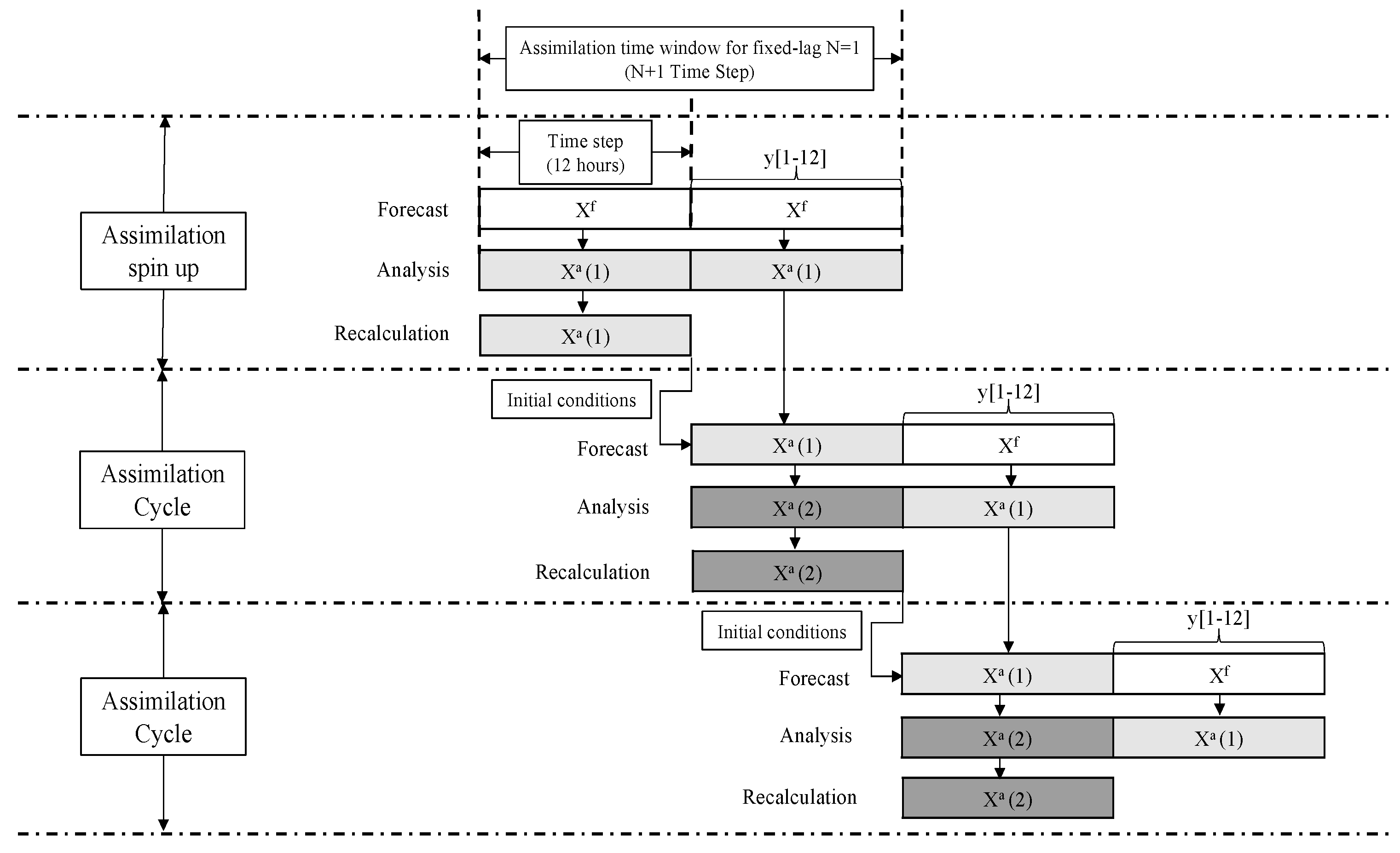
We implement a fixed-lag Ensemble Kalman smoother (EnKS) into the WRF-Chem (version 3.5.1) [16] to invert the dust emissions. ‘Inversion’ is used here for an approach where the dust emissions, simulated with a model, are back-calculated or optimized by assimilating observations. As shown in Figure 1, a fixed-lag EnKS with a parameter lag of value N spans a time window of (N + 1) time steps, and the state vector contains the variables to be optimized (i.e., dust emissions here) for (N + 1) time steps [8]. In this study, we optimize the dust emissions every 12 h, which corresponds to each time step of 12 h; this is the convenient option used for the preparation of the hourly emission inventories for WRF-Chem using two emission files for the emissions of 0–11 h and 12–23 h, respectively. Each assimilation cycle advances a time step, and the dust emissions for all the (N + 1) time steps are optimized using only the observations within the last time step. After each assimilation cycle, the dust emissions for the first time step are the final optimized results, which have been optimized (N + 1) times and will no longer be optimized in the next cycle. The finally optimized dust emissions therefore serve as the forced dust emissions for advancing the system one time step, and they provide the initial conditions for the next assimilation cycle. The analyzed dust emissions, excluding those for the first time step combining the new predicted dust emissions, become the background state vector for the next cycle. The first guess dust emissions (i.e., a priori) are parameterized with the Air Force Weather Agency (AFWA) dust emission scheme for the Goddard Ozone Chemistry Aerosol Radiation and Transport (GOCART) aerosol model within the WRF-Chem [17]. The uncertainty of a priori dust emissions (i.e., model errors) is considered by perturbing the dust emissions to create the model ensemble simulations with 20 members. The perturbation factors are drawn from a lognormal distribution, with a mean equal to 1.0 and a standard deviation equal to 0.6. The standard deviation of 0.6 corresponds to the uncertainty of the dust emissions for 14 global models [4]. To avoid the cancellation effect, the emission perturbations are generated in relation to the model grids and do not vary with time [18,19].

Like the above-mentioned method, it is apparent that a fixed-lag EnKS with lag N repeatedly corrects the dust emissions with observations from that time step up to N subsequent time steps. The EnKS solves an analysis equation very similar to that of EnKF but with time lags between the analysis and innovations (observations minus forecast) [20]. To efficiently assimilate the hourly aerosol observations from the next-generation geostationary satellite Himawari-8 [21], we apply a four-dimensional local ensemble transform Kalman filter (4D-LETKF) to solve the Kalman equations [22]. With each assimilation cycle, the 4D-LETKF finds the maximum likelihood solution of dust emissions from the following Kalman equations:

$$x^a=x^f+P^a·H^T·R^{-1}·\left(y-H·x^f\right)$$

(1)

$$P^a={\left(I+P^f·H^T·R^{-1}·H\right)}^{-1}·P^f$$

(2)

where the state vectors $x^f$ and $x^a$ are the mean dust emissions of the so-called priori and posterior ensembles, respectively; the $P^f$ and $P^a$ are the error covariance matrices of the priori and posterior dust emissions, respectively, which are estimated and evolved through the ensemble simulations; the vector $y$ denotes the assimilated hourly Himawari-8 AOD observations with a horizontal resolution of 0.5° × 0.5° after aggregate preprocessing [22]; the $R$ is the observation error covariance matrix, which is assumed to be diagonal and estimated as the sum of the instrumental error variance and the sample error variance; and the operator $H$ (i.e., WRF-Chem) relates the a priori dust emissions to the forecasts of the simulated observations. An important advantage of local ensemble transform Kalman filter (LETKF) is its localization, which reduces the spurious error covariance with distance due to the limited ensemble size and enables the parallel processing [9]. This localization is utilized in the observation error covariance by multiplying the inverse of the localization function with the observational error covariance, as in Dai, Cheng, Suzuki, Goto, Kikuchi, Schutgens, Yoshida, Zhang, Husi, Shi and Nakajima [22]. The localization factors are given by the Gaussian function:

$$f\left(r\right)=\exp \left(-r^2/2{\sigma }^2\right)$$

(3)

where $\sigma$ is the localization length defined as the physical length (km), and $r$ is the physical distance between the local patch center and the position of the assimilated observation. The function has the effect that the influence of the observations on the analysis at a location decays gradually with an increasing distance to the analysis. The fifth-order piecewise rational function is used to truncate the infinitely long tails of the Gaussian function [23]. It drops to zero at:

$$r=2·\sqrt{10/3}·\sigma$$

(4)

that is, we do not assimilate observations beyond that distance.

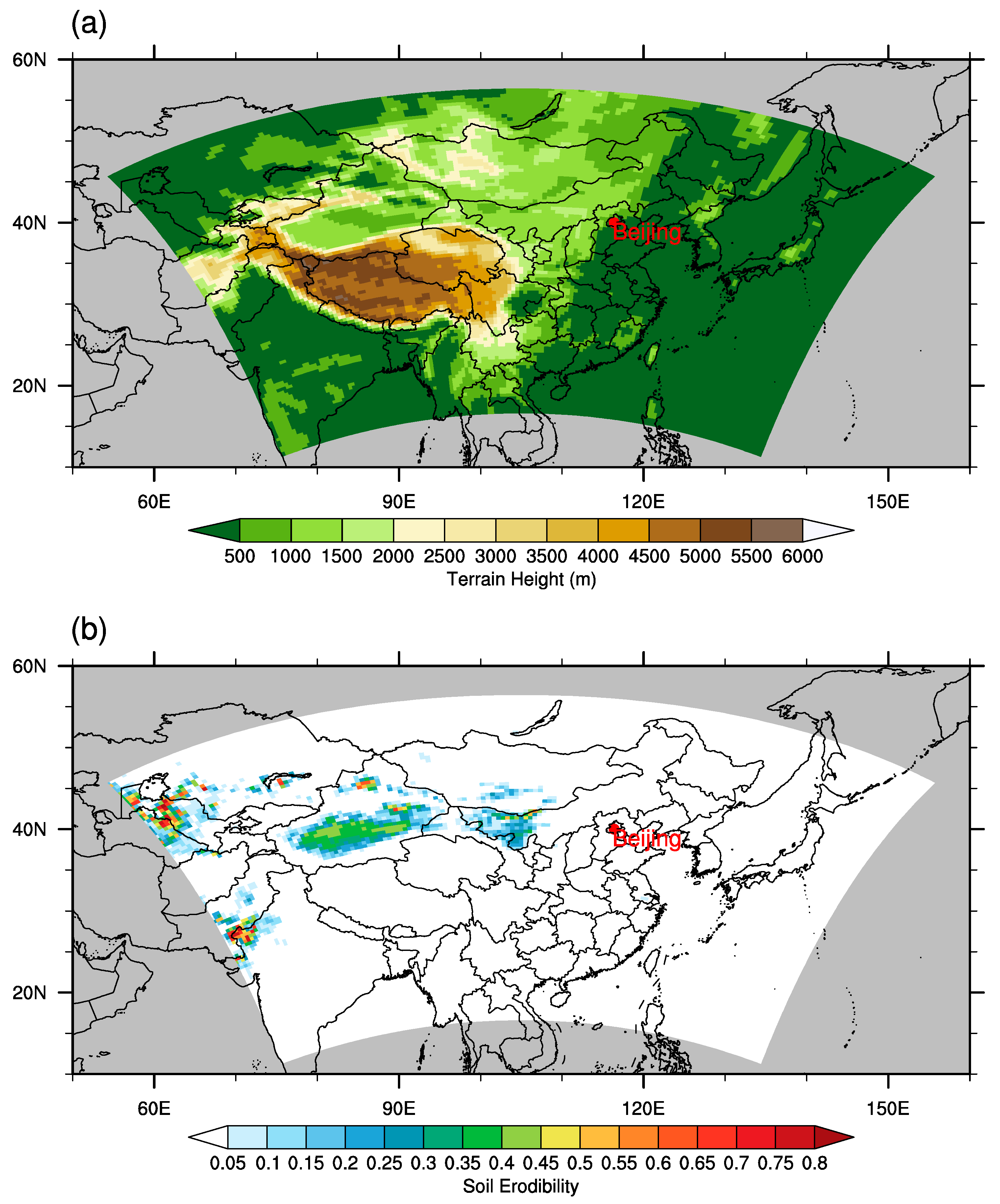
The WRF-Chem is configured with a domain that has a horizontal resolution of 45 km, as shown in Figure 2. The terrain height and soil erodibility over the domain are also shown in Figure 2a,b, respectively. The vertical resolution is 28 layers from 1000 mb to 100 mb. The main selected physics are the Noah land surface module [24], the Mellor-Yamada-Janjic (MYJ) Planetary Boundary Layer (PBL) scheme [25], the sophisticated Lin microphysics [26], and the Rapid Radiative Transfer Model (RRTM) radiation scheme [27]. The assimilated Himawari-8 AODs include the contributions of all the aerosol components, and we cannot separate the dust AODs from the other aerosols. Therefore, the aerosol simulation should treat both the dust and non-dust aerosols. In light of the computational resources, the aerosol simulation is based on the simple GOCART aerosol scheme [28,29]. The main tropospheric aerosols, including dust, sea salt, organic carbon, black carbon, and sulfate, are considered in the emissions and predicted mass mixing ratios. To compare it with the Himawari-8 retrieved AODs, the simulated AOD is calculated with the WRF-Chem “aerosol chemistry to aerosol optical properties” module, assuming that the particles are spherical and internally mixed with all the simulated aerosol components [30]. Since the watering of the dust particles may significantly affect the light-scattering properties [31], the hygroscopicity parameter Kappa is used to represent the aerosol hygroscopic growth, and the multicomponent hygroscopicity parameter is computed by weighting the component hygroscopicity parameters by their volume fractions in the mixture [32]. However, to limit the inversion information, only the dust emissions are perturbed and optimized in this study.

A control experiment without assimilation (Free Running, or FR simulation hereafter) is performed as a reference. Five assimilation experiments are performed to study the effects of the assimilation and the system parameters (i.e., localization length and lag) on the dust emission inversions and model performances. The parameter localization length determines the assimilated observations in the horizontal space. With a larger localization length, more observations can be assimilated for the analyses at a grid point, but the spurious error covariance with distance may deteriorate the analyses. The parameter lag determines the assimilated subsequent observations. More subsequent observations can be assimilated with a larger lag, but more computation time is required. The first three experiments use one time step lag (i.e., an assimilation time window of 1 day) and localization lengths of 45 km (L45kmT1d simulation hereafter), 300 km (L300kmT1d), and 600 km (L600kmT1d), respectively. The last two experiments use an assimilation time window of 2 days and localization lengths of 300 km (L300kmT2d) and 600 km (L600kmT2d), respectively. All of the simulation experiments start from 00:00 UTC on 23 November 2016 with a spin-up period of 2 days, and the inversions of the dust emissions are investigated for the period of 25–27 November 2016, during which a severe winter dust event in East Asia occurred. The model performances against the observations are measured via the statistical metrics, including the mean error (Bias) [33], the root mean square error (RMSE), the correlation coefficient (R), the index of agreement (IOA) [34], and the skill score (Skill) [35].

3. Results

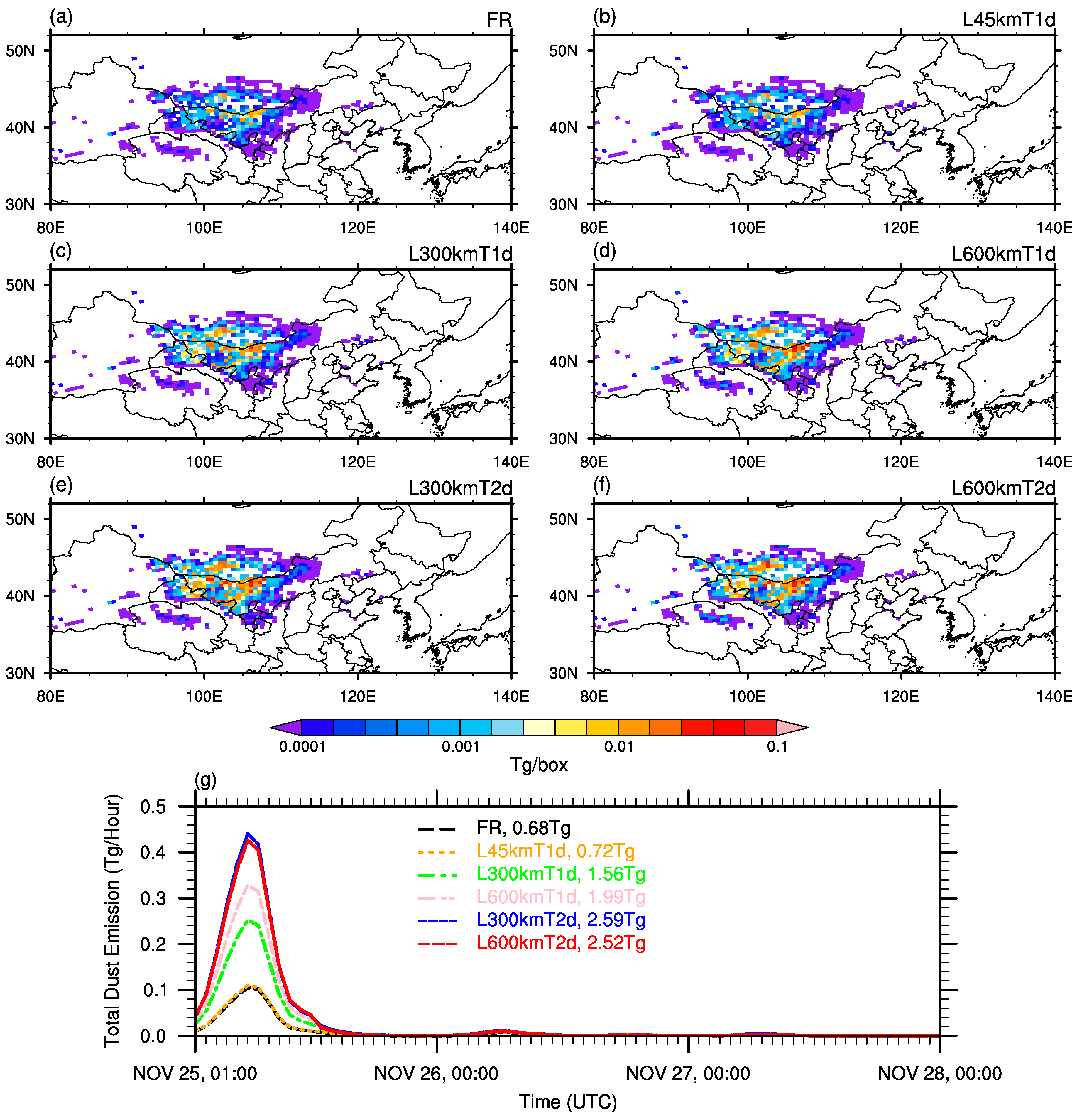
Figure 3a–f shows the horizontal distributions of the priori and posterior accumulated dust emissions during 25–27 November 2016, and Figure 3g shows the time series of the hourly total dust emissions over the region 30° N–52° N and 80° E–140° E. The dust emissions from this event are primarily from the Gobi Desert, with a peak value at 06:00 UTC on 25 November. Since the dust emission perturbations are invariant with the model grid and time, the priori and the posterior dust emissions show generally consistent spatial and temporal patterns. The L45kmT1d experiment has similar dust emissions as the FR simulation because there are only a few observations over the dust source areas on 25 November for the inversion (see Figure 4). Ideally, the mean of the ensemble assimilation with no assimilated observations should be equal to that of the FR simulation. The sensitivity study reveals that the parameter lag has a larger effect on the inverted dust emissions than the parameter localization length, and the total dust emissions are converged for the L300kmT2d and L600kmT2d experiments, with values of 2.59 Tg and 2.52 Tg, respectively.

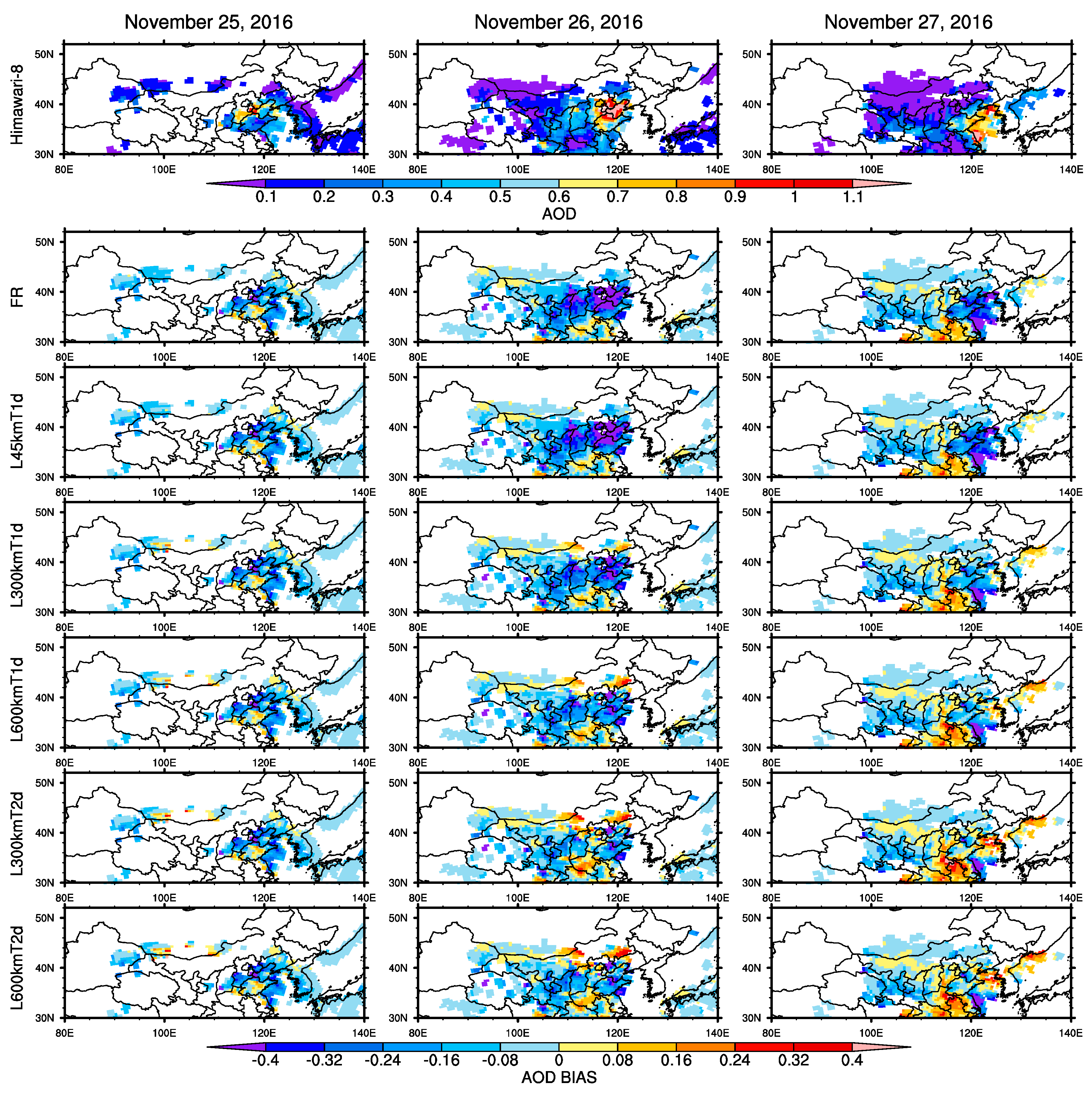
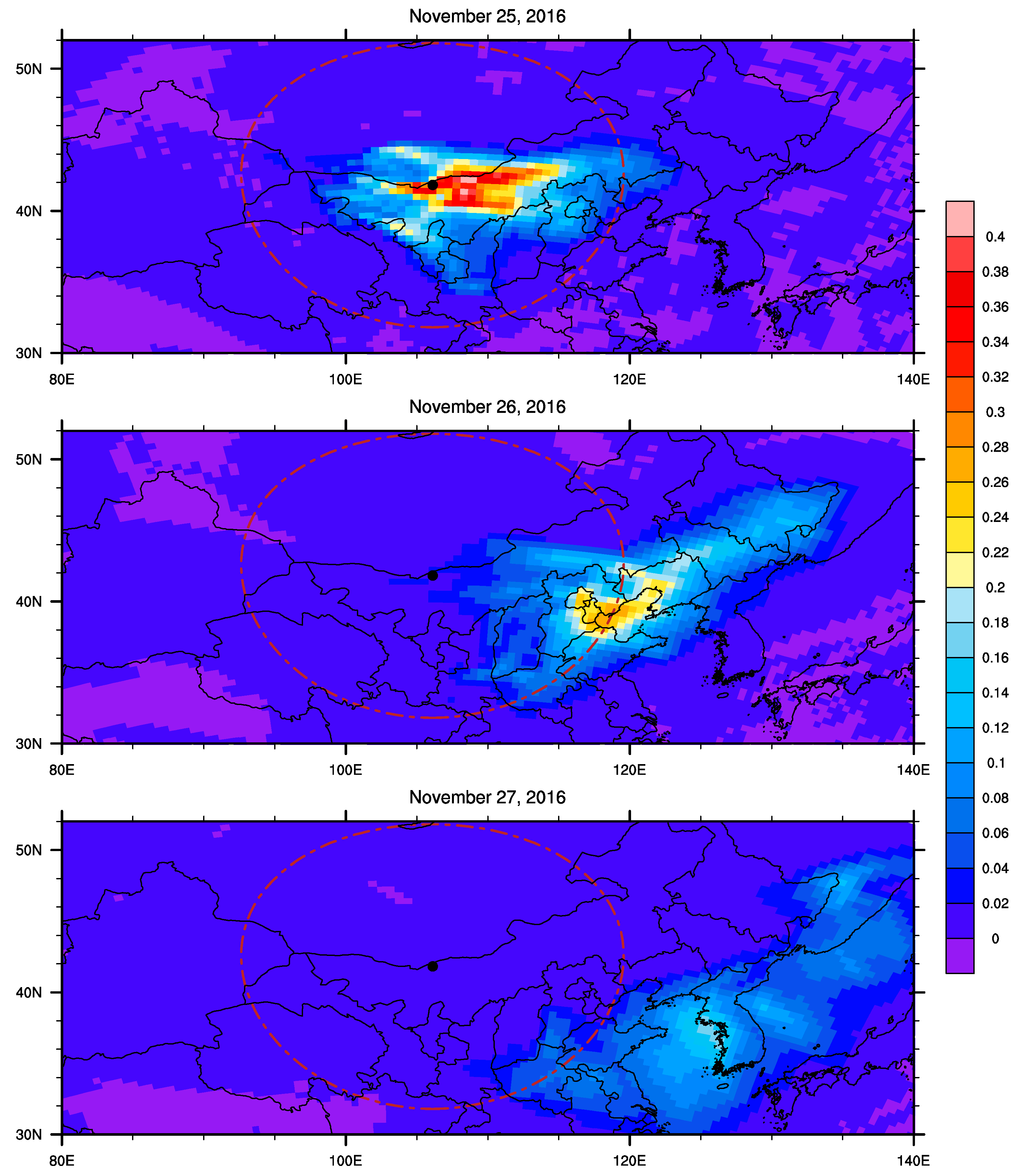
Figure 4 further shows the horizontal distributions of the daily averaged Himawari-8 AODs for 25–27 November 2016 and the mean biases between the simulated and Himawari-8 observed AODs. The emitted dusts are transported eastwardly, resulting in higher Himawari-8 AODs surrounding the Bohai and Yellow Seas on 26 and 27 November, respectively. The WRF-Chem can generally capture the dust transport processes, especially on 26 November, as shown in Figure 5. Himawari-8 reveals two AOD hotspots on November 27 surrounding the Yellow Sea and the west coast of North Korea, whereas the predicted dust is generally transported to the west coast of North Korea, as indicated by the higher values of the normalized model error covariances in Figure 5. This indicates that, due to the transport process, the model error generally grows with the dust travel distance [2]. The simulated AODs over the dust outflow areas in the FR experiment are generally lower than the observations, indicating that the dust emissions are underestimated. Underestimations of the dust emissions over the Gobi Desert are also found in other dust models [7]. The model simulated dust emissions are mainly dependent on the wind speeds at a 10 m height, the soil moisture, and the snow cover, and it is difficult for the model itself to correctly estimate these parameters. Consequently, the estimated dust emissions do not yield a good performance. A detailed probing of the underestimations of the dust emissions is beyond the scope of this study. All of the assimilation experiments, in particular those with an assimilation time window of 2 days, increase the dust emissions to reduce the negative AOD biases, as is the case over the Bohai Sea areas on 26 November. As given in

Table 1. The statistical results of the simulated aerosol optical depths (AODs) over 25–27 November 2016 in the six experiments versus the Himawari-8 observed ones. The statistics, including the mean error (Bias), root-mean-square errors (RMSE), correlation coefficient (R), index of agreement (IOA), and skill score (Skill), are calculated between 30° N–52° N and 80° E–140° E. There are 17,650 pairs of simulated and observed AODs used to calculate the metrics. The number in bold indicates the best model result.

Experiment	Bias	RMSE	R	IOA	Skill
FR	−0.111	0.223	0.700	0.700	0.574
L45kmT1d	−0.110	0.221	0.705	0.703	0.578
L300kmT1d	−0.085	0.197	0.744	0.786	0.719
L600kmT1d	−0.072	0.189	0.745	0.814	0.781
L300kmT2d	−0.047	0.186	0.733	0.837	0.837
L600kmT2d	−0.054	0.185	0.741	0.836	0.831

, the statistical metrics reveal that the model performances of all the assimilation experiments are superior to those of the FR experiment, and that the L300kmT2d experiment generally represents the best results with the lowest Bias and highest IOA and Skill. This indicates that the simulations with dust emission inversions exhibit an improved consistency with the observations and hence provide a positive check on the emission inversion system. Compared to the experiment with an assimilation time window of 1 day, the experiment with a time window of 2 days generates a better simulation and is generally unaffected by the parameter of localization length. This is because the inverted dust emissions with an assimilation time window of 1 day are further optimized by the observations on the next day for a time window of 2 days, indicating that an assimilation time window of 1 day is not enough for the dust emission inversion. As shown in

Table 2. Same as Table 1, except for 27 November 2016 only and 7311 pairs of simulated and observed AODs used for calculating the metrics.

Experiment	Bias	RMSE	R	IOA	Skill
FR	−0.086	0.218	0.701	0.702	0.549
L45kmT1d	−0.085	0.217	0.705	0.706	0.555
L300kmT1d	−0.055	0.197	0.719	0.787	0.713
L600kmT1d	−0.041	0.194	0.713	0.807	0.768
L300kmT2d	−0.012	0.199	0.698	0.824	0.827
L600kmT2d	−0.021	0.195	0.707	0.825	0.820

, the general underestimations of the AODs over the Shandong Province and its surrounding areas in the FR experiment on 27 November are also reduced in the assimilation experiments. This reveals that the dust predictions over 3 days also benefit from the inverted dust emissions on 25 November, since the observations on 27 November are not used for the inversions of the dust emissions on 25 November, even with an assimilation time window of 2 days.

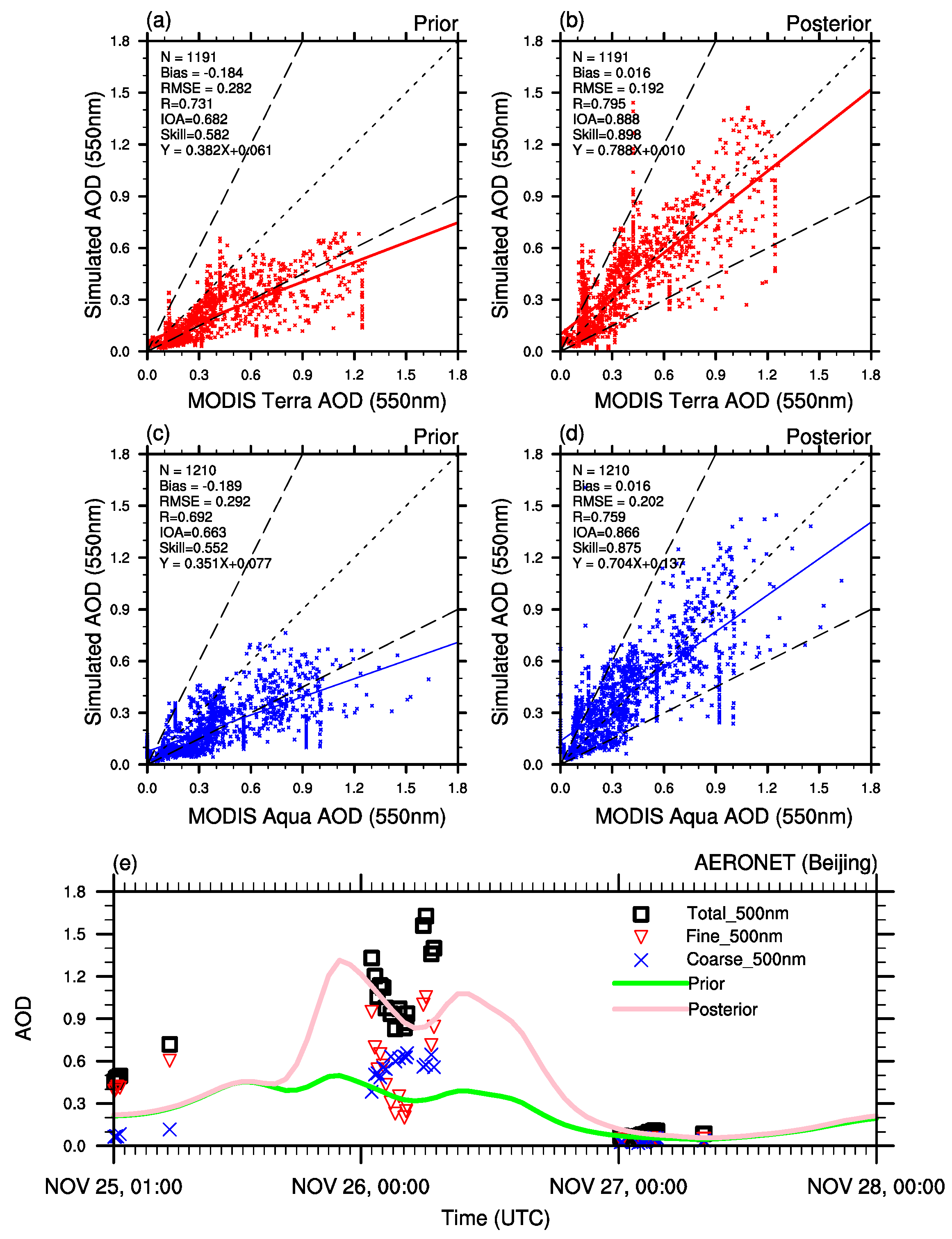
As shown in Figure 6, the simulated AODs of the FR and L300kmT2d experiments are validated by the independent observations from Collection 6.1 of Moderate Resolution Imaging Spectroradiometer (MODIS) [36] and Version 3 Level 2.0 of Aerosol RObotic NETwork (AERONET) [37]. It is apparent that the simulated AODs with priori dust emissions are generally lower than the observed AODs from both the MODIS Terra and Aqua satellites. The simulated AODs with the posterior dust emissions from the L300kmT2d experiment are much more comparable to the observations, as all of the statistical metrics are improved. This indicates that the posterior dust emissions improve the model simulations when compared to the independent MODIS observations. It is worth noting that only the grids dominated by the dust aerosols are here used for the validation because the emissions of non-dust aerosols are not optimized in this study, and the grids are defined as the simulated AODs between the FR and L300kmT2d experiments having relative differences greater than 40%. The AERONET-observed AODs over the Beijing site reveal that the emitted dust is transported to Beijing early on 26 November, as indicated by the relatively high total and coarse mode AODs. The simulated AODs with the priori dust emissions are significantly lower than the AERONET-observed total AODs and even lower than the coarse mode AODs early on 26 November, whereas the simulated AODs with the posterior dust emissions generally reproduce the magnitude and variation of the AERONET-observed AODs. This further proves that the inversion system can optimize the dust source emissions to better represent the dust transport processes.

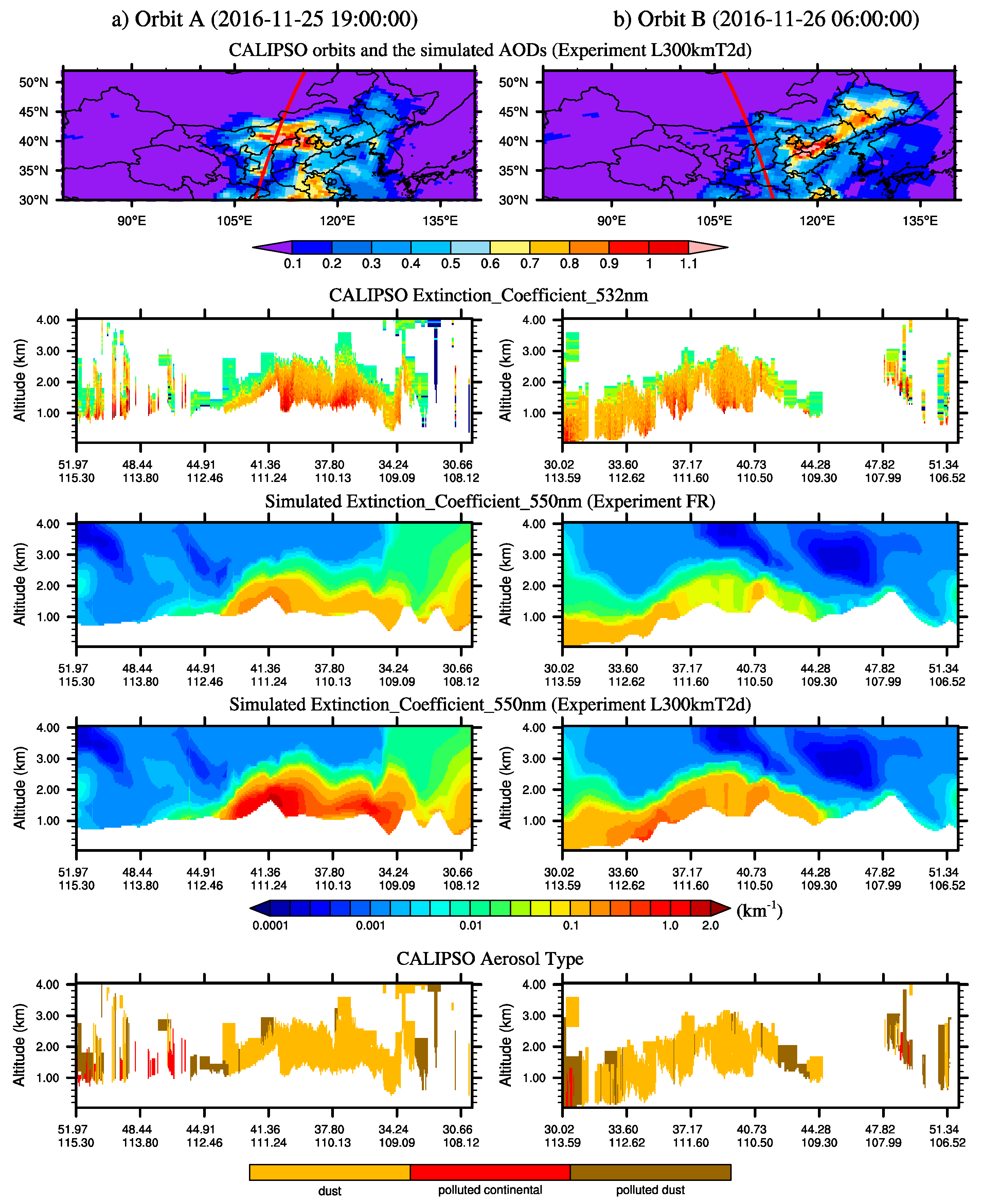
Figure 7 further shows the independent validations with the retrieved aerosol extinction coefficients from the Cloud-Aerosol Lidar with Orthogonal Polarization (CALIOP) onboard the CALIPSO [38]. There were two CALIPSO orbit paths over or near the Gobi dust source region during 25–26 November that could detect the vertical distributions of this dust event. The horizontal distributions of the simulated AODs indicate that the A and B paths detect the vertical distributions of the aerosol extinction coefficients during and after the dust event, respectively. The vertically resolved distributions of the CALIPSO aerosol types reveal that the aerosol types in both the A and B paths are mostly dust. Although the vertical patterns of the simulated aerosol extinction coefficients of both the A and B paths are similar to the CALIPSO-observed patterns, the FR experiment tends to underestimate the aerosol extinction coefficients both during and after the dust event, while the L300kmT2d experiment reproduces a magnitude and variation that is more reasonable. These results indicate that the FR experiment reproduces the dust emission height and downward transport quite well but that it underestimates the dust emission fluxes; therefore, the enlarged posterior dust emissions enhance the magnitude of the dust processes and induce better agreements with the CALIPSO observations.

4. Conclusions

We developed and applied an aerosol emission inversion system, which is based on the fixed-lag ensemble Kalman smoother and the WRF-Chem model, to optimize dust emissions during a severe winter dust event in East Asia in November 2016. The assimilated observations were the hourly AODs retrieved from the next-generation geostationary meteorological satellite Himawari-8. Sensitivity studies were also performed to investigate the potential effects of the system parameters (lag and localization length) on the dust emission inversions.

The dust emissions of this severe winter dust event were primarily from the Gobi Desert, with a peak value at 06:00 UTC on 25 November. The Asian dust was transported eastwardly, arriving at Beijing early on 26 November and causing AOD hotspots over the Bohai and Yellow Seas on 26 and 27 November, respectively. The simulated AODs with the priori dust emissions were clearly lower than the assimilated Himawari-8 AODs and the independent MODIS and AERONET ones, indicating that the priori dust emissions were underestimated. The posterior total dust emissions were more affected by the assimilation time window than the localization length and converged with a time window of 2 days. The posterior total dust emissions with best model performances were 3.8 times higher than the priori emissions, with values of 2.59 Tg and 0.68 Tg.

The simulated AODs with the best posterior dust emissions were much more comparable to the assimilated Himawari-8 and independent MODIS and AERONET observations than to those with the priori dust emissions; for example, the simulation skill scores improved from 0.574, 0.582, and 0.552 to 0.837, 0.898, and 0.875 for Himawari-8, MODIS Terra and Aqua, respectively. With the posterior dust emissions, the simulated vertical distributions of the aerosol extinction coefficients, both during and after the dust event, were also more consistent with the independent CALIPSO observations than to those with the priori dust emissions. It was also shown that the dust predictions could also benefit from the inverted dust emissions.

The dust perturbation factors were assumed to be invariant with the model grid and time, due to the limited ensemble size, and this induced the inversion system to generally only optimize the magnitudes of the dust emissions but not the spatial and temporal patterns. The uncertainties of the non-dust aerosol emissions and other aerosol processes, such as transport, chemical reaction, and deposition, were not considered in this study’s dust emission inversions, and this may have caused a particular uncertainty in the dust inversion. When more computational resources are available, future work should be conducted to determine a better way to generate the model errors to eliminate such negative effects.