Gravity Waves in Planetary Atmospheres: Their Effects and Parameterization in Global Circulation Models


1
Max Planck Institute for Solar System Research, 37077 Göttingen, Germany
2
Department of Physics and Astronomy, Space Weather Lab, George Mason University, Fairfax, VA 22030, USA
*
Author to whom correspondence should be addressed.
Atmosphere 2019, 10(9), 531; https://doi.org/10.3390/atmos10090531
Submission received: 11 August 2019
/
Revised: 31 August 2019
/
Accepted: 4 September 2019
/
Published: 9 September 2019
(This article belongs to the Special Issue Modeling and Simulation of Planetary Atmospheres)
Abstract
:The dynamical and thermodynamical importance of gravity waves was initially recognized in the atmosphere of Earth. Extensive studies over recent decades demonstrated that gravity waves exist in atmospheres of other planets, similarly play a significant role in the vertical coupling of atmospheric layers and, thus, must be included in numerical general circulation models. Since the spatial scales of gravity waves are smaller than the typical spatial resolution of most models, atmospheric forcing produced by them must be parameterized. This paper presents a review of gravity waves in planetary atmospheres, outlines their main characteristics and forcing mechanisms, and summarizes approaches to capturing gravity wave effects in numerical models. The main goal of this review is to bridge research communities studying atmospheres of Earth and other planets.
1. Introduction
Gravity waves (GWs) are ubiquitous in planetary atmospheres. Their fundamental role in the dynamics and global circulation was first recognized for the middle and upper atmospheres of Earth. GWs generated in lower and denser atmospheric layers propagate upward carrying energy and momentum. Since their amplitudes increase with height due to the exponential drop of pressure, nonlinearity eventually takes over and limits the growth, or even causes waves to break down. Other dissipative processes, among which molecular diffusion and thermal conduction are the most prominent in the thermosphere, add to wave damping. The deposited momentum and energy deliver a significant amount of dynamical and thermal forcing on the thin air. It drives many atmospheric phenomena and circulation features and, therefore, cannot be ignored at all. GWs play a fundamental role in the dynamics of planetary atmospheres by redistributing momentum and energy between the layers, mainly from the bottom up, thus providing vertical coupling between them [1].
Capturing effects of GWs in numerical global (or general) circulation models (GCMs) presents a challenge. These waves have horizontal scales from tens to hundreds of kilometers, which are often smaller than the resolution of GCMs. Moreover, instabilities and breaking processes occur at scales much smaller than the wavelength. Even present-day GCMs with very high resolution cannot so far simulate details of these processes. Thus, effects of GWs must be parameterized in the models. Over the last few decades, the role of GWs was increasingly appreciated in the terrestrial atmosphere, and the numerical means of accounting for wave effects in GCMs were greatly advanced. Details of the related progress can be found in several comprehensive reviews e.g., [2,3].
Observations provide ample evidence that GW activity is very strong in the atmospheres of planets of the terrestrial group (Mars and Venus) and apparently even stronger on Jupiter. This brings the necessity to account for their effects in a growing number of atmospheric GCMs for planets other than Earth. The main focus of this paper is to review the recent progress with understanding the role of GWs in planetary atmospheres and outline the approaches of accounting for them in GCMs. One of the paper’s goals is to bridge the gap between the research communities studying atmospheres of Earth and other planets.
The structure of the paper is the following. In Section 2, we give a concise description of the GW physics and the corresponding linear theory, outline available observations and characterize parameters and sources of GWs in planetary atmospheres. Principles of parameterization of GWs in numerical models and existing closure concepts are discussed in Section 3. Various effects of GWs and approaches to their modeling are reviewed in Section 4. Phenomena associated with GWs in planetary atmospheres as modeled in GCMs are presented in Section 5. Concluding remarks are given in Section 6.
2. Atmospheric Gravity Waves
2.1. Physics of Gravity Waves
Gravity waves appear in fluids with varying density as a result of oscillations of neighboring parcels around their equilibrium positions. Since forces that counteract vertical displacements of parcels are gravity and buoyancy, the waves are alternatively called gravity or buoyancy waves. To sustain the oscillations, the fluid must be convectively stable. A well-known example of a stratified fluid is the ocean surface, which represents an interface between denser water and thinner air. Gravity waves that propagate horizontally along it are called “surface waves”. Atmospheres are continuously stratified by density. Therefore, atmospheric GWs are also able to propagate vertically. To signify this distinction from surface waves, the latter are called “internal” waves.
The fundamental quantity that characterizes properties of the stratified air is the Brunt-Väisälä (or buoyancy) frequency N, with which parcels oscillate vertically:
where g is the acceleration of gravity, is the potential temperature related to the absolute temperature T as , R is the gas constant of air, is the specific heat capacity at constant pressure p, is a standard (reference) pressure. Air parcels rarely oscillate only in the vertical direction, but have horizontal displacements as well. Their orbits are thus tilted ellipses. The longer the horizontal excursion of the parcel is, the longer it takes to return to the initial state. Therefore, periods of internal GWs depend on the ratio of the vertical and horizontal wavelengths, or on the vertical angle of phase propagation. On the shortest-period end of the spectrum (, or a few minutes on planets of the Solar system), there are almost vertically propagating harmonics, for which pressure gradient force enters the balance. These waves are called “acoustic-gravity”. The longest-period end of the GW spectrum is occupied by harmonics with large horizontal extents and time scales close to rotational periods of the planets. They are affected by the inertial force in addition to buoyancy and gravity, and are called “inertia-gravity” waves. Large-scale and low-frequency waves are often resolved by GCMs, while the impact of high-frequency acoustic-gravity waves on general circulation can, in many cases be neglected. Hence, we do not focus on the two extremes in our consideration that follows.
2.2. Linear Theory of Gravity Waves
The derivation of the dispersion relation for linear GWs can be found in many texts, for instance, in Section 2.1 of the review paper of Fritts and Alexander [2]. For that, it is assumed that all field components participating in GW oscillations can be represented as a sum of individual harmonics proportional to , where m is the vertical wavenumber, is the angular frequency as seen from the ground, and are the horizontal wavenumbers in the zonal and meridional directions, correspondingly. The dispersion relation connects frequencies and wavenumbers and has the form
In Equation (2), , is the horizontal wave vector, is the intrinsic frequency, or the frequency of the harmonic observed in the frame of reference moving with the speed of the background wind. This dispersion relation does not include any dissipative terms yet. The other quantities in Equation (2) describe the background characteristics of the atmosphere: is the Coriolis parameter, is the rotational frequency of the planet, is the latitude, is the scale height of the background (undisturbed) density . In conservatively propagating internal GWs, magnitudes of air parcel displacements and amplitudes of all wave field variables grow exponentially with height as , to compensate for the density drop (locally, ).
For vertically propagating GW harmonics, which are of the most interest in the context of this paper, and m are real. The latter can only occur if . For planets such as Earth or Mars, the intrinsic frequency spans the range of two orders of magnitude. It also strongly varies as the wave propagates through a vertical shear. Negative (imaginary m) indicates that the wave decays vertically and is called evanescent. When m approaches zero, the harmonic undergoes total internal reflection. At small m (large vertical scales), the density change over the vertical wavelength (the effect of compressibility) is significant and the term becomes important.
If effects of rotation are neglected (), the relation Equation (2) yields for the intrinsic horizontal phase speed in the direction of wave propagation
Normally, horizontal extents of atmospheres are much larger than vertical ones, and so are horizontal vs. vertical wavelengths (). It follows from Equation (3) then
It is seen from Equation (4) that is the largest at the reflection point . This provides a useful and simple characteristic of GWs in planetary atmospheres - the maximum horizontal phase velocity . For all known planets in the Solar system, is smaller than the speed of sound, the expression for which under the ideal gas approximation has the form , where is the ratio of specific heat capacities at constant pressure and constant volume. As can be judged from the quantities entering the two expressions, there is no fundamental reason for the speed of GWs being always subsonic. This means that the frequency separation between acoustic and gravity waves is not a fundamental atmospheric feature. A caution must be taken with applying the existing theoretical framework to the rapidly growing number of discovered exoplanets.
Table 1 presents typical parameters of some planetary atmospheres of the Solar system that pertain to GW characteristics. For instance, periods of vertically propagating GWs on Venus can exceed those on fast rotating outer giants by three orders of magnitude (). Horizontal phase speeds of fastest waves on gas giants can exceed those in the atmospheres of terrestrial planets by a factor up to 10. GWs with vertical scales shorter than the scale height of a planet are of the most interest for parameterizing in GCMs.
Further simplification of the dispersion relation can be obtained for GWs with mid-range intrinsic frequencies and for which :
where is the horizontal phase speed in the frame of reference related to the ground. It demonstrates strong dependence of GW properties on the background wind and stability N. In particular, the level where (and ) is called critical, because harmonics cannot propagate through it. In the real atmosphere, instabilities and enhanced dissipation destroy the waves upon approaching a critical level.
2.3. Wave Generation and Sources of Gravity Waves
Vertical displacement of parcels is the necessary condition for GW excitation. There are many processes in planetary atmospheres that force air to move vertically and, thus, can potentially generate GWs. Some of the conspicuous but infrequent sources are volcano eruptions, earthquakes, meteorites, tsunamis, and hurricanes. However, most of GWs are excited in the lower atmosphere by flow over topography, convection, and instability of weather systems.
Since orographic GWs are steady in the planetary frame, they have zero or very small horizontal phase speeds. In the Earth stratosphere, they create “hot spots” of wave activity tied to particular geographical features [4]. The Martian surface is much rougher and near-surface winds are stronger than on Earth. Simulations using Martian GCMs with increased resolution clearly demonstrate enhanced wave activity over mountainous regions [5,6,7,8]. A large bow-shaped stationary GW signature was observed at the cloud tops of Venus [9]. It is believed to be generated in the lower atmosphere over the large mountain feature and then propagated upward. Orographic sources are usually better parameterized in GCMs, primarily because the topography is well known. Very often modelers distinguish orographic and “non-orographic” GW parameterizations based on that.
Convection is a more prominent mechanism of wave generation, because many atmospheric regions, mainly in the troposphere, have low static stability. Convective plumes overshoot and trigger stable layers either mechanically (penetrative, dry convection), or through heat release (moist convection). The latter is particularly abundant in Earth’s tropics. Strong heating of the Mars surface creates temperature inversions, which are subject to various convective phenomena such as dust “devils” [10], “plumes” [11] and “cells” [12]. Tropospheres of Venus and Jupiter are also known regions of convective activity causing GW generation [13]. This mechanism produces predominantly short GWs with horizontal scales determined by sizes of the convective structures and/or their envelopes.
Weather phenomena are not limited to particular regions and are apparently the major source of GWs in planetary atmospheres. Instability and transience of jets and front systems systematically create vertical displacements of air of various scales. An insightful review of the related mechanisms is given in the work by Plougonven and Zhang [14]. Weather on Mars, Venus and, especially, Jupiter [15] is more volatile than that on Earth. Simulations with high-resolution GCMs show that the seasonal variations of GW activity both in the lower and upper atmospheres of Mars are tightly linked with the behavior of the circumpolar vortex and its instability, in particular [8].
2.4. Observations of Gravity Waves
All field variables participate in oscillations induced by GWs. Therefore, observations of, at least, one of them allows for deducing many wave characteristics. A variety of techniques has been used to detect GW signatures in the terrestrial atmosphere. They include in situ measurements, when sensors directly contact the air, and ground- and space-based remote sensing. The examples of the ground-based techniques are incoherent radars detecting reflection from density fluctuations, meteor radars using ionization of air by meteors, pulsed lasers called LiDARs, or receivers of the Global Navigation Satellite System (GNSS) signals that experience refraction and reflection during propagation. An example of a new and rapidly developing method is the infrasound tomography of GW structures [16]. Orbital-based instruments scan the atmosphere from the top down at different spectral intervals.
For obvious reasons, applications of ground-based remote sensing techniques for atmospheres of planets other than Earth are extremely limited. We are unaware of their applications to GWs to date. Given the relatively small scales of GWs, their signatures are difficult to detect from Earth’s surface or orbits. Therefore, the most of information on GWs in planetary atmospheres has been collected from space missions, either from orbiters, or descending probes. Thus, first vertical profiles with GW signatures have been obtained from the Viking 2 entry data on Mars [17], from the Galileo probe on Jupiter [18] and Huygens probe on Titan [19]. Examples of other in situ techniques are mass-spectrometer measurements of wave-like structures in the upper atmosphere of Venus [20] and VEGA balloon experiment in the Venusian middle atmosphere [21].
While spacecraft entries are very rare, in situ measurements from orbiters can provide significantly more information about GWs in the upper atmospheres. Spacecraft perform aerobraking operations to form their orbits by dipping into the denser layers. The collected accelerometer data can be used to infer density variations along the trajectory. Thus, horizontal spectra of GWs have been obtained in the Martian thermosphere from the aerobraking data of Mars Global Surveyor (MGS) and Mars Odyssey (ODY) [22,23].
Mass-spectrometers onboard orbiters is another powerful in situ method of measuring GWs. Using observations of neutral gas density during Cassini’s flybys over Titan, Müller-Wodarg et al., [24] detected GW-like disturbances in the thermosphere with vertical wavelengths greatly exceeding the scale height. In the thermosphere of Mars, an extensive study of GWs is being performed using data from Neutral Gas and Ion Mass Spectrometer (NGIMS) onboard the Mars Atmosphere and Volatile Evolution (MAVEN) orbiter. In particular, it was shown that the observed wave features are consistent with upward propagating GWs originated in the lower atmosphere [25], that wave amplitudes are systematically damped with height by convective instability [26] and that the wave activity strongly varies with seasons and diurnally [27].
Sounding deeper into the atmosphere requires remote sensing approaches. Radio occultation is a technique particularly suitable for detecting GWs with relatively small spatial scales. Transponders with ultra-stable frequencies installed on orbiters transmit radio signals, which are then detected by Earth-based receivers. While passing through the atmosphere during occultation events, radio signal experiences refraction and absorption. One can sense the atmospheric properties by their influences on the radio frequency. This method provides vertical profiles of temperature and density with resolution much smaller than the scale height e.g., [28,29]. It allowed for deriving vertical wavenumber spectra of GWs on Mars [30] (using the data from MGS) and on Venus [31] (from the Venus Express data). The spectra turned out to be remarkably similar to those on Earth: their high-m spectral tails decay according to the power law and amplitudes (scaled by ) were close. The “universality” of the vertical wavenumber spectra are tightly linked to breaking and/or saturation of GW harmonics ([2] Section 4.2) and, thus, provides evidence of unceasing wave influence on the atmosphere.
We next consider how small-scale GWs affect the large-scale atmospheric flow and how these processes can be parameterized in GCMs.
3. Methods of Parameterizing Gravity Waves in General Circulation Models
3.1. Principles of Parameterization
Parameterizations always represent simplifications that result in loss of accuracy. If parameterizations are to be distinguished from errors, they must (1) be preferably based on laws of physics (first principles), rather than on a set of ad hoc tunable parameters; (2) be verifiable in the sense that the quantities they provide can be compared against observations; (3) the number of tuning factors that arise from neglected or unknown physics must be kept to a minimum. We next outline the assumptions and approximations that most of GW parameterizations currently used in GCMs are based on.
GW schemes parameterize the impact of small-scale waves on a larger-scale flow, rather than the wave field itself. For that, the information about wave phases is neglected and only averages of quadratic quantities are considered instead. The most commonly used ones include variance/energy, vertical flux of horizontal momentum or simply momentum flux , sensible heat flux , etc., where the individual perturbation quantities describe the departure of a field variable from its average, in accordance with Reynold’s decomposition, e.g., . The averaging (“coarse-graining”) denoted by the bar is taken over model’s grid scales, which are larger than the wavelengths of harmonics of interest.
Waves are excited at all heights; however the amplitudes of those propagating downward exponentially decrease with altitude and so does their influence on deeper and denser layers. Therefore, only waves traveling upward must be considered. This also allows the neglect of harmonics that experience full reflection on their way up. Since reflection takes place at small m (see Section 2.2), the short vertical scale approximation excludes such harmonics, thus allowing for application of the Wentzel–Kramer–Brilloin (WKB) method. Fast GWs (with long vertical wavelengths) are less affected by diffusion and have more chances to penetrate the thermosphere. A care must be taken, when the WKB approximation is applied to GWs in the thermosphere.
GWs propagate obliquely with respect to the surface with the phase tilt determined by the ratio . Horizontal propagation can be neglected for harmonics with short vertical wavelengths (). In the majority of operational GW schemes, waves are assumed to propagate within a vertical column and in one model timestep. Limitations of such approach have been discussed in the work of Kalisch et al., [32] and parameterizations using ray-tracing have been proposed in the work by Song and Chun [33].
With the approximations outlined above, a general scheme for parameterizing GW drag produced by a harmonic i can be summarized as follows. The equation of conservation of wave momentum flux (per unit mass)
is solved upward, given the value of the flux at the source level and a parameterization for the vertical damping rate are provided. The divergence of the flux yields the acceleration/deceleration (per unit mass) of the mean flow in the direction of harmonic’s horizontal phase speed or, as it is loosely called, the GW “drag"
It is seen from Equations (6) and (7) that, if the wave propagates conservatively (), it produces no net drag and it does not affect the background mean flow. Thus, quantification of the vertical damping rate is of primary importance for parameterizing effects of subgrid-scale GWs. The other important step is prescribing/parameterizing wave sources at a certain level in the lower atmosphere. In the rest of this section, we overview the existing closures for .
3.2. Instability Threshold
Instability theories study the response of a fluid flow to some initial perturbations. One form of stability is the static stability (or vertical stability), which is essentially a question of whether an air parcel is colder or warmer than its environment and depends highly on the vertical distribution of temperature. The static stability is judged by the relation:
where is the potential temperature, is the dry adiabatic lapse rate, and is the ambient lapse rate, where the lapse rate describes the rate at which the temperature decreases with increasing altitude. If , then , meaning that an upward displacement cools the air parcel more than the environment, leading to a buoyant force that pushes the parcel down to its original position. This condition is a stable equilibrium configuration or a static stability case. If , then , leading to a statically unstable condition. Then, a lifted air parcel would continue to rise. An unstable atmosphere is an extremely short-lived condition. Usually turbulence or convection mixes the air vertically until stable conditions are established.
In a realistic atmosphere, wind, temperature, and mass density vary as a function of height. Kelvin–Helmholtz instabilities can occur at the interface of two fluids of different mass densities in the presence of winds shear. GWs within these shear layers can become unstable and break, depending on their amplitudes. This phenomenon often occurs in the lower atmosphere and can be observed in billow clouds. At higher altitudes, it is obvious that wave amplitudes cannot grow infinitely with height and nonlinearity must suppress the growth at some levels. One of the first concepts suggested by Hodges [34] assumes that waves become unstable at sufficiently large amplitudes such that enhanced turbulence produces damping, which offsets further growth and maintains the amplitude at the threshold value. This closure has been implemented first by Lindzen [35] and later reviewed by Fritts [36] and Dunkerton [37]. The diffusion occurs suddenly when the harmonic’s amplitude reaches either the convective instability threshold
or that of dynamical (Kelvin–Helmholtz) instability . In general, convective instability occurs when the buoyancy frequency is imaginary, while Kelvin–Helmholtz instability requires the presence of strong wind shear. Overall, dynamic instability is more common for wave frequencies , while convective instability predominates GWs in the midfrequency range, which most GW parameterizations assume. The advantages of this approach are that (1) it is based on a simple physical concept and (2) produces reasonable magnitudes of GW drag. It must be noted that, to achieve the latter, all Lindzen-type of parameterizations must apply the so-called “intermittency factor”, which effectively reduces the mean flow acceleration by several times. The verbal justification for the introduction of the tuning intermittency factor is that GWs exist only a part of time. This is a questionable argument, because waves are considered on time steps much shorter than the periods of waves and the assumed time averaging (denoted by the bar) has already taken care of possible irregularities. The disadvantages of applying convective/dynamical instability thresholds are the following. (1) A sudden onset of instability causes vertical profiles of wave drag to be step-functions. This creates continuity problems for large-scale models. Many parameterizations of that kind had to introduce artificial smoothing extending the action of the drag below the breaking level. (2) The saturation theory requires wave amplitudes to be nearly constant above the breaking level, while detailed simulations show that waves can be completely destroyed during the break-up [38].
3.3. Spectral Schemes
In a quest to overcome the above-mentioned problems with the Lindzen-type parameterizations, Alexander and Dunkerton [39] extended this approach by considering a broad spectrum of GWs and including a significantly larger number of harmonics. The waves were assumed to propagate independently without dissipation until they reach their respective breaking levels determined by the convective instability thresholds. Total internal reflection at high intrinsic frequencies was taken into account. Unlike in the original Lindzen scheme, breaking harmonics deposited all their momentum at once (similarly to that in [40]) and ceased to exist. This approach smooths somewhat over the vertical profiles of the resulting momentum forcing, but does not eliminate discontinuities completely and still requires an “intermittency” factor to achieve reasonable magnitudes of the GW drag. More importantly, the parameterization does not account for saturation and, since breaking harmonics are eliminated, cannot reproduce the saturated slope of the vertical wavenumber spectrum.
Warner and McIntyre [41] applied a less aggressive damping at the instability threshold levels. They assumed that when the energy/amplitude of a harmonic meets the saturated value of the “universal” vertical wavenumber spectrum, its growth with height is halted and dissipation removes the surplus wave momentum (per unit mass) to accelerate the mean flow. At certain cases, the damping can be strong enough to obliterate the wave. Warner and McIntyre [42] have developed a more computationally effective hydrostatic (see Equation (5)) version by employing piecewise continuous spectra and Scinocca [43] has produced a discretized variant of [42]. Although these schemes are called “spectral”, propagation of each component is considered separately. Unlike with [39], they produce smoother vertical profiles of GW drag suitable for large-scale models by spreading momentum deposition among many harmonics. These parameterizations also require tuning primarily associated with the choice of frequency spectrum, which is difficult to constrain with observations.
However, the biggest problem with these schemes is the applicability of the “universal” spectrum saturation criterion in the presence of the mean wind . The latter strongly distorts the vertical wavenumber spectra due to Doppler shifting. Majdzadeh and Klaassen [44] have thoroughly investigated the behavior of the parameterizations [42,43] and demonstrated that they never can reproduce the saturated slope in the background shear, even if it was prescribed by the saturation criterion. This poses a question of whether the empirical threshold of the “universal” spectrum can be used in the presence of the mean wind at all. In addition, the above schemes treat critical line filtering as an abrupt obliteration of harmonics, thus imposing momentum deposition at one point and providing a nonphysical strain on numerical models. Clearly, some explicit physical mechanisms for wave dissipation are required. There are two theories have been offered to date. The corresponding parameterizations are considered in the next subsection.
3.4. Nonlinear Spectral Schemes
Hines [45] offered the Doppler spread theory (DST), according to which interactions between waves produce net Doppler spreading of all spectral components to higher vertical wavenumbers. Once a harmonic’s vertical wavelength becomes sufficiently short, the wave is obliterated by an unspecified mechanism, presumably by molecular diffusion. The Doppler spread parameterization (DSP) [46] simplifies the DST by assuming that (a) spread of harmonics can be represented by Doppler shift, (b) harmonics are obliterated when shifted beyond a prescribed cut-off wavenumber, and (c) the shift can be approximated by rms wind created by all waves thus that the denominator in Equation (5) takes the form , where is the rms wind of waves directed along the phase velocity , is the rms wind of all harmonics, and and are tuning parameters. This expression shows some similarities with the convective instability threshold Equation (9), where the amplitude of a single harmonic is replaced by the spectrum-induced wind variance. It is also seen that the DSP essentially describes enhanced critical level absorption when harmonics start to deposit momentum before reaching their linear critical levels.
Charron et al., [47] have shown that the GW drag produced by DSP was systematically stronger than that of [42] for the same conditions. McLandress and Scinocca [48] argued that the DSP could be further tuned, such that the averaged fields simulated by a GCM using different GW schemes were close. Majdzadeh and Klaassen [44] noted that the DSP could not reproduce the saturated slope of the vertical wavenumber spectra in the absence of mean wind shear (similar to the scheme of [39]), because the large-wavenumber harmonics were progressively obliterated. The DST is based on the assumption that waves are conservative and non-interacting in the Lagrangian frame of reference and become nonlinear when transformed to the Eulerian frame [49]. The physical and mathematical foundations of the DST were tested in the works of Klaassen and Sonmor [50], Klaassen [51], and Klaassen [52]. It was shown that the entire picture of Doppler spreading was based on a physically flawed model violating conservation of mass and energy. To date, the DSP remains a heuristic scheme that has no theoretical and physical ground.
An alternative theory of nonlinear interactions within broad spectra of GWs was developed by Weinstock [53] and Weinstock [54] and further advanced in the work by Medvedev and Klaassen [55] (MK95). According to the theory, harmonics with periods longer than of a test wave act as a spectrum-induced background producing Doppler shift reminiscent of that in the DST. Components with vertical wavenumbers larger than cause instabilities on scales shorter than the wavelength of the test wave. When averaged as outlined in Section 3.1, these effects act as diffusion limiting the wave amplitude. Under certain conditions, the test harmonic itself can become unstable and obliterate.
For purposes of parameterization, the spectrum-induced Doppler shifting can be neglected and the vertical damping rate takes a simple analytical form [56]
where is the rms wind created by all shorter vertical-scale () waves in the spectrum. If the spectrum is represented by a single (nonlinear selfinteracting) harmonic, the MK95 reduces to a straightforward generalization of the Lindzen scheme [35]; however, the predicted onset of breaking/saturation occurs continuously and at smaller amplitudes with the proportionality coefficient depending on and the background conditions. For spectra containing many harmonics, the damping starts at even lower heights (and smaller amplitudes). The calculated momentum forcing is, thus, smaller (see Equation (7)) and the parameterization requires no further tuning with “intermittency” factors. Similarly, the MK95 scheme continuously treats the momentum deposition by waves approaching critical levels. The last but not least, the parameterization self-consistently reproduces the observed features of “universal” spectrum, including the saturated slope of the high-wavenumber tail, its magnitude, and the evolution with height of the lowest vertical wavenumber m affected by the saturation vertical wavenumber ([55] Figure 3).
3.5. Whole Atmosphere Gravity Wave Scheme
With the development of GCMs extending into the thermosphere (“Whole Atmosphere models”) up to the exobase, a need for suitable GW parameterizations has emerged. While nonlinear processes of breaking/saturation are the main mechanisms for transferring wave energy and momentum to larger-scale flows in the lower and middle atmosphere, other factors strongly affect dissipation of GWs in the upper atmosphere. The major contribution to wave damping comes from molecular diffusion, thermal conduction, and ion friction. Other important mechanisms that limit the exponential growth of amplitudes are eddy diffusion and radiative damping. Since these factors act together, they can be conveniently included in GW parameterizations by putting in Equation (6) to
where the terms in the right-hand part denote vertical damping rates due to nonlinear breaking/saturation, molecular diffusion, and thermal conduction, ion friction, eddy/turbulent diffusion, and radiative damping, correspondingly. The most comprehensive “whole atmosphere” GW parameterization to date has been developed by Yiğit et al., [57]. It includes the MK95 spectral scheme. A number of parameterizations is also described in detail in the work of Yiğit and Medvedev [58].
This parameterization can be directly applied to atmospheres of other planets, where conditions can significantly differ from those on Earth. The atmosphere of Mars almost completely consists of carbon dioxide. Eckermann et al., [59] argued that radiative transfer in IR bands of CO imposes much stronger damping on GWs than on Earth and hypothesized that wave amplitudes can be reduced upon propagation upward, such that they do not reach breaking/saturation levels. The effect of radiative damping of GWs on Mars has been modeled using the whole atmosphere scheme [57]. It demonstrated that radiative damping dominates only in the lower atmosphere, where other effects are small, and that it results only in small changes in the GW drag in the middle and upper atmosphere ([60] Section 7).
Interactions of neutrals with ions in the thermosphere produce wave damping only in the presence of planetary magnetic field. A recently developed update to the whole atmosphere GW scheme is the novel parameterization of wave damping by ion friction [61]. It shows that dissipation of GW harmonics is strongly anisotropic and depends only on the geometry of the magnetic field, but not its strength. Thus, the scheme can accurately parameterize effects of GWs in GCMs covering thermospheres of planets with intrinsic magnetic fields, such as Earth or Jupiter.
3.6. Stochastic Modifications of Parameterizations
The above described parameterizations represent the wave field as a superposition of many independent (Section 3.2 and Section 3.3) or interacting (Section 3.4) monochromatic GWs. Further modifications of the existing schemes have been directed at increasing their computational efficiency. Instead of considering the full set of harmonics, Eckermann [62] proposed to launch only one wave at each model time step by randomly choosing its spectral characteristics and amplitude with fixed probability distribution at the source level. Since periods of GWs are usually much longer than the time steps, Lott et al., [63] improved the formalism by launching a few monochromatic waves (wave packets) at a time and by redistributing the calculated GW drag over much longer time scales.
The stochastic versions of their corresponding “full spectrum” prototype GW schemes produce much more sporadic instantaneous forcing; however, the average simulated fields turn out to be close in both cases. There were attempts to link the stochastic parameterizations to the intermittency of observed GWs e.g., [64]; however, the randomness did not eliminate the need for tunable “intermittency” parameters [65]. We note again that the latter had to be introduced to substitute for imperfections of the underlying theories of GW breaking/saturation.
4. Modeling Gravity Wave Effects in Planetary Atmospheres
Having considered approaches to parameterizing GWs, we now turn to their effects in the atmosphere, mainly in the context of numerical model studies. GWs affect the momentum and energy budget of the background atmosphere as well as distributions of atmospheric species. This influence is referred to as dynamical, thermal, and mixing effects, respectively. Most of the studies of interest have been performed for atmospheres of Earth and Mars, hence, they dominate in this section.
4.1. Dynamical Effects
Studies of momentum forcing, or GW drag (Equation (7)), were greatly motivated by the need to explain the observed reversed summer-to-winter meridional temperature gradient in the mesosphere of Earth. Differential absorption of solar radiation in the summer and winter hemispheres would lead to a thermally induced transport cell and, through the Coriolis force, to strong easterly and westerly jets, correspondingly, extending throughout the middle atmosphere and thermosphere. Leovy [66] was the first who, with the help of a simplified GCM, realized that some sort of mechanical dissipation was required to balance this strong zonal acceleration to explain the observed circulation in the middle atmosphere. This required dissipative force was linked to GWs breaking up in the mesopause region. Considering turbulence accompanies the violent breaking processes [34,67], Leovy [66] parameterized it by the Rayleigh friction
with being the coefficient that was later assumed to vary with height [68]. Damping of this form was able to partially compensate for the Coriolis torque induced by the meridional circulation and close the jets in both hemispheres in simulations with middle atmosphere GCMs, in accordance with observations. The importance of subgrid-scale GWs in maintaining the momentum budget in the upper mesosphere was thus recognized, albeit the reversal of the jets in the mesosphere and lower thermosphere could not be reproduced by the models using Equation (12). This became possible only with the introduction of more sophisticated and physically based parameterizations [35,69], which have been discussed in Section 3. In particular, it was shown that the reversals are accompanied by the coldest region in the Earth atmosphere—in the Sun-lit summer polar mesosphere [70].
Further progress with quantification of the GW momentum forcing in GCMs was made due to advances with parameterizations and obtaining more observational constraints on the GW activity and spectra at all atmospheric levels [71,72]. These were mainly middle atmosphere altitudes, as were the upper lids of model domains of majority of GCMs until 2000s. With the development of the so-called “whole atmosphere models”, whose upper boundaries extend into the upper thermosphere, the need for proper GW parameterizations have emerged. Initially, it was thought that most of GWs break down below the turbopause (at ∼105 km on Earth), and those that survive the propagation upward are rapidly damped by exponentially increasing molecular diffusion and thermal conduction. On the other hand, there was ample observational and modeling evidence that GWs of tropospheric origin reach thermospheric heights and have significant amplitudes there e.g., see the review by Yiğit and Medvedev [1].
The gap in understanding the GW role in the dynamics of the upper thermosphere has been systematically addressed using the “whole atmosphere” parameterization [57] implemented into the Coupled Middle Atmosphere-Thermosphere-2 (CMAT-2) model. It was acknowledged [73] that not all GWs are absorbed in the middle atmosphere and some waves propagate into the thermosphere, where they experience increased dissipation [74,75]. This agreed with direct simulations using a partially GW-resolving whole atmosphere GCM (T85, ) [76], which demonstrated that GW forcing is important and cannot be neglected in the momentum budget of the thermosphere. Figure 1 presents the zonal mean zonal GW drag () simulated by the CMAT2-GCM during the Northern Hemisphere solstice (at low solar and geomagnetic activity), using the whole atmosphere scheme. Panel a illustrates the approach of most middle atmosphere GCMs by cutting off the GW drag at around the turbopause. Panel b is from the extended simulation, in which GWs were allowed to propagate into the thermosphere and dissipate, producing a significant drag there, especially at higher altitudes. Panels c and d serve for comparison of another major force in the upper thermosphere–the ion drag. It is seen that global effects of GWs occur nearly at all latitudes and heights from 70 to 240 km, and that the mean zonal GW and ion drags have the same order of magnitude. Later GCM studies with the whole atmosphere scheme demonstrated substantial GW effects on the migrating diurnal tides in the mesosphere and thermosphere [77].
Besides using GW parameterizations in coarse-grid GCMs, advanced numerical wave models have been extensively applied for studying various aspects of propagation of GW packets from the troposphere to the upper atmosphere and produced momentum forcing [78,79,80,81]. They demonstrated that harmonics with longer vertical wavelengths dominate at higher altitudes, because their smaller vertical gradients are less affected by molecular diffusion. Meanwhile, it has been proposed that GWs breaking in the middle atmosphere can themselves serve as a source of higher order harmonics (e.g., secondary waves) [82,83]. Wave models can greatly help in establishing how effective this mechanism is and, if so, in implementation of such sources in GW parameterizations.
Gravity waves shape the dynamical structures of other planetary atmospheres as well [84]. Studies of the dynamical importance of GWs in the atmospheres of other planets started almost immediately after the emergence of corresponding GCMs. On Mars, dynamical effects of GWs were studied systematically since the 1990s e.g., [85,86,87,88,89]. They used simplified Lindzen-type GW schemes (see Section 3.2) and focused almost exclusively on orographically generated GWs with zero horizontal phase speed (except for [86]). Motivated by the similarity of the thin Martian atmosphere and the terrestrial thermosphere, and the success of the broad-spectrum GW parameterization in Earth GCMs e.g., [73,90], Medvedev et al., [60] performed off-line tests of the scheme under Martian conditions and found indications that circumpolar jets must reverse in the middle atmosphere. Simulations with a Martian GCM interactively incorporating the parameterization revealed a strong dynamical influence of small-scale unresolved GWs on the circulation and state of the Martian atmosphere between 100 and 130 km [91]. The produced zonal mean GW drag was found to be in the order of hundreds of m s sol in both hemispheres (leading to the reversals of the middle atmosphere jets, as predicted), while instantaneous values could reach thousands of m s sol, in agreement with the estimates based on measurements [22,23]. Recent, GCM simulations in combination with MAVEN observations showed that GWs play an important role in thermospheric dynamics and structure of the wave number-3 structure in Mars’ thermosphere [92].
The effects of GWs on the variation of wind velocity in the Venusian lower thermosphere have been investigated using several GCMs. It was suggested that accounting for GW drag can help to match the simulated subsolar-to-antisolar (SS-AS) winds with observations [93]. The latter study included a simplified Rayleigh-drag parameterization given by Equation (12), while others employed more sophisticated parameterizations. In particular, Zalucha et al., [94] employed the Alexander and Dunkerton [39] scheme and found that GWs did not propagate above 115 km due to the internal reflection. Using the MK95 (Section 3.3) scheme, Hoshino et al., [95] demonstrated that GWs drive the retrograde super-rotation zonal (RSZ) winds in the night side around 110 km by providing the westward momentum at higher altitudes. Gilli et al., [96] used a stochastic parameterization [63] and showed that GWs noticeably improve simulations near the terminator.
4.2. Thermal Effects
Wind and temperature fields are interrelated in the atmosphere, therefore dynamical forcing can affect the thermal state as well. A prominent example of this is the absolute temperature minimum in the summer polar mesosphere of Earth caused by the adiabatic cooling due to GW-enhanced ascent branch of the meridional circulation. Thermal effects considered in this subsection result from the direct influence of waves on temperature. Dissipating/breaking GWs irreversibly transfer their mechanical (kinetic and potential) energy to heat. This heat deposition is, in principle, analogous to Joule heating in electromagnetic processes. Another effect that accompanies wave dissipation was first described in the work by Walterscheid [97]. In conservatively propagating GWs, fluctuations of vertical velocity and temperature are in opposite phases, thus that the average vertical flux of the sensible heat . If amplitudes of fluctuations decay with height, as is in the case of dissipating GW harmonics, and do not cancel, and the net flux is no longer zero, but directed downward. Thus, the second type of thermal effects of GWs is the downward transport of sensible heat. Divergence of the flux yields cooling rates above and heating rates below the levels affected by dissipation.
Consideration of the energy budget of GWs interacting with the mean flow reveals that both processes can be easily parameterized for a harmonic with in terms of the produced wave drag ([98,99] eqn. (36’)):
with and R being the specific heat and gas constant, respectively. Due to the density stratification, cooling rates (per unit mass) in the second term of Equation (13) above the breaking/dissipating level exceed the heating below, and the dominant effect of GWs is cooling the upper atmosphere. Incorporation of the parameterization Equation (13) in the whole atmosphere scheme within a terrestrial GCM resulted in GW-induced cooling in the thermosphere of about 100 K day in an average sense, thus bringing the simulated temperature closer to observations [100]. Instantaneously, the cooling rates can occasionally exceed 1000 K day. After molecular thermal conduction, GWs are the second-largest cooling mechanism that maintains the stability of the thermosphere.
In the context of planetary atmospheres, the thermal effects of GWs were studied in a lesser extent. The parameterization Equation (13) has been implemented into a Martian GCM [101] to explain the temperature structure measured during the Mars Odyssey aerobraking experiment [102]. These observations had shown unexpectedly cold temperature in the Martian lower thermosphere down to 100 K. Figure 2 illustrates that the inclusion of thermal effects of GWs (together with the dynamical forcing by GWs) is likely responsible for the observed cold night-time temperatures (red dashed line vs blue dotted one). Cooling by GWs in the Martian atmosphere has been studied further in comparison with the radiative cooling due to IR transfer in CO molecules [103]. The latter are the main components in the atmosphere of Mars, and their emission in IR represents a major radiative cooling mechanism, especially in the rarefied air of the upper atmosphere. It was shown that the GW-induced and radiative cooling rates are comparable in the lower thermosphere, although the former increase with height. More measurements of atomic oxygen, which facilitates cooling under the break-up of local thermodynamic equilibrium (non-LTE), are required to constrain the radiative cooling rates.
Another application of direct thermal effects of GWs is related to the Jovian thermosphere, which is hotter than that follows from radiative balance calculations. Based on the detection of GW-like structures in the thermosphere of Jupiter, heating rates (first term in Equation (13)) have been calculated and shown to be sufficient for explaining the temperature difference [18]. However, later, Hickey et al., [104] applied a full-wave model and demonstrated that the contribution of GWs is relatively small and that, depending on the damping by molecular diffusion, the result can be cooling instead of heating. The latter is in line with accounting for the second term in Equation (13), whose magnitude depends on the vertical profile of the GW drag that, in turn, is determined by the dissipation mechanisms. It was suggested that dissipating acoustic waves can heat the thermosphere [105]. Acoustic waves are poorly constrained in both terrestrial and Jovian atmospheres, and they are beyond the scope of this paper.
5. Phenomena Associated with Gravity Waves in Planetary Atmospheres
GWs are most known for their impact on the mean wind and global circulation. In this section, we outline a few other atmospheric phenomena, in which the waves in question play a substantial role.
5.1. Sudden Stratospheric Warmings
As the name suggests, a sudden stratospheric warming (SSW) is the process of rapid increase of stratospheric temperature in the winter hemisphere of Earth, which was discovered and first described in [106]. Major and minor SSWs take place in the Northern hemisphere, while minor warmings occasionally occur in the Southern hemisphere during Antarctic winters. SSWs are accompanied by the slowing down the zonal mean eastward winds in case of minor warmings and even by their reversals during major events. It is generally established that sudden enhancements of planetary waves (PWs) with zonal wavenumbers 1 and 2 in the troposphere and lower stratosphere are responsible for the initiation of the warmings [107,108,109,110]. The interhemispheric difference in SSW occurrences is due to the dissimilarity of surface characteristics and, thus, of PW activity.
Since propagation and dissipation of GW harmonics are functions of the intrinsic horizontal phase speed , changes in the zonal mean wind during SSWs greatly affect the GW activity at layers above the stratosphere itself [111]. GCM simulations with the implemented GW parameterization demonstrated a complex feedback between the GW activity, forcing, and circulation in the stratosphere and thermosphere during a minor SSW event [112]. In particular, the GW activity in the middle thermosphere (in terms of wave-induced wind fluctuations) can increase by up to a factor of three. The changes in activity produce alternating spatio-temporal patterns of forcing, which modulate larger-scale (resolved by GCMs) thermospheric wind variability by up to [113]. GW-induced coupling between the stratosphere and thermosphere during SSWs are not fully understood and yet to be studied with measurements and modeling [114]. In particular, based on GPS-TEC observations, it was demonstrated that the ionospheric GW activity declined at the initial phase of the stratospheric jet reversal during the major warming of 2008/2009 winter [115]. A similar decrease of the GW activity at middle atmospheric altitudes was found in TIMED-SABER observations [116].
5.2. Martian Polar Warmings
Unlike the transient and sudden events in the terrestrial atmosphere, Martian polar warmings are persistent features that last for entire seasons. They represent vertical reversals of temperature over winter poles between 50 and 80 km and have magnitudes of several tens of Kelvin degrees. Similar to Earth’s mesosphere, where a reversed meridional temperature gradient exists, the middle atmosphere of Mars over winter poles has been found to depart from a radiative equilibrium, much unlike the polar atmosphere below. It was recognized that these polar warmings are caused dynamically rather than by radiative processes [117,118], namely by the adiabatic heating due to the downward branch of the global meridional circulation cell.
Figure 3 illustrates the simulated warming over the southern winter pole. White streamlines present the global meridional transport descending over the pole and inducing strong adiabatic heating. The zonal-mean circulation is maintained by large-scale non-zonal disturbances (eddies)-solar tides and planetary waves. Red lines in Figure 3b show the transport of the eddy energy up from the lower atmosphere (Eliassen–Palm fluxes), while the momentum forcing (the divergence of the fluxes) is given by blue lines. The magnitude of the polar warming increases during global dust storms. This increase occurs due to the strengthening of the solar tides and the meridional circulation cell driven by them [118]. Similarly, large-scale GW activity increases during dust storms and contributes to the polar warming [120].
Inclusion of a parameterized forcing by subgrid-scale GWs enhances the middle atmosphere polar warmings; however, its main effect occurs in the lower thermosphere, where a similar type of polar warming has been observed at around 100–130 km [102,121]. The analysis of in situ aerobraking data in the Martian lower thermosphere indicated that this high-altitude polar warming is much stronger during the perihelion season [102]. Its magnitude also depends on the dust opacity in the lower atmosphere [122], even though the latter does not directly affect radiative processes in the thermosphere. Simulations accounting for the effects of subgrid-scale GWs led to an enhancement of both the middle and upper atmosphere winter polar warmings ([123] (Figure 11)), thus demonstrating their tight link to GWs.
5.3. Gravity Waves and Ice Clouds
Carbon dioxide clouds have been frequently observed in the Martian middle atmosphere e.g., [124,125]. Since the latter is generally warmer than the CO condensation threshold, Clancy and Sandor [124] hypothesized that clouds can form in pockets of cold air that occasionally occur due to superposition of temperature fluctuations induced by GWs and tides. Reproducing formation, distribution, and characteristics of CO clouds with GCMs was challenging for modelers because of the sub-grid size of the pockets. Nevertheless, simulations with the Laboratoire de Météorologie Dynamique (LMD) GCM demonstrated that although condensation temperatures were never achieved, the spatial and temporal distributions of cold air correlated with observations of CO clouds [126]. They were created in the model only by thermal tides, because GWs were neither resolved, nor included in a parameterized form. The role of waves was addressed using a mesoscale (GW-resolving) limited area model [5]. The authors directly demonstrated that GWs generated by the flow over topography can propagate to the upper mesosphere and create patches of air at supersaturated temperatures there.
To explain global distributions of CO clouds, simulations have been performed with the Max Planck Institute (MPI) MGCM using the implemented “whole atmosphere” spectral scheme (see Section 3.5) [127]. Since the GW parameterization keeps track of all harmonic’s amplitudes at each grid point, but does not describe the instantaneous wave field itself, the RMS of GW-induced temperature fluctuations can serve as a probabilistic measure of CO cloud occurrence. The clouds can form, if the total of the simulated (large-scale) temperature T and the parameterized GW disturbances drops below the saturated threshold : (. These simulations shown in Figure 4 reproduced higher probability of cold pocket occurrences in the lower latitudes of the mesosphere during the vernal equinox (around ), in accordance with observations of CO clouds. They also demonstrated distinct diurnal variations of the pockets due to modulation by tides. In addition, the simulations predicted more clouds than observed at higher altitudes and in polar regions.
Simulations over a Martian year [128] have shown that GWs facilitate CO cloud formation in two ways. First, they cool down the upper atmosphere globally (by ∼9% in the mean sense). Second, they create cold patches of air as described above. The model also predicted high probabilities of clouds during the second half of the Martian year (–), which was not substantiated by observations until writing this review. However recently, mesospheric CO clouds have been detected at ∼100 km in southern summer [129]. Apparently the mechanism of cloud formation is more complex and involves microphysical processes in addition to cold temperatures. Nucleation processes strongly depend on sizes (and existence) of dust nuclei particles, and CO condensation may require supersaturated temperatures up to several tens degrees below the condensation threshold [130,131]. Although the role of GWs in CO cloud formation is firmly established, the precise mechanisms that control their occurrence on Mars are still the subject of intense research.
5.4. Ionospheric Effects
The ionosphere is a partially ionized outermost portion of a planetary atmosphere, where neutrals and ions coexist and interact. Typically, the neutral part (thermosphere) is much denser, e.g., the terrestrial thermosphere is about 100 times denser than the F region ionosphere. As GWs propagate through the thermosphere and perturb neutrals, they can influence ions as well. Overall, effects of GWs in the ionosphere are still understood insufficiently, especially in the context of ionospheres of other planets. The work of Hines [132] is one of the first that associated irregularities in different ionospheric regions with neutral GWs. In particular, large-scale traveling ionospheric disturbances (TIDs) of electron density were interpreted as a response to the passage of GWs e.g., [133].
Kirchengast et al., [134] have pointed out the necessity of detailed numerical modeling for understanding the connection between TIDs and atmospheric GWs. A numerical model was used for identifying characteristics of ionospheric disturbances generated by different sources and comparing with those of observed individual TIDs [135]. The latter can be subdivided into two major categories: large-scale (horizontal wavelength ∼1000 km) fast moving TIDs (horizontal phase speeds ∼250 m s) with periods ∼1 h, and medium-scale ones (∼100 km, 100 m s, 10 min, respectively) [136]. The former are usually the manifestation of GWs generated by a variety of processes in the upper atmosphere, such as Joule heating, particle precipitation, electric field variability, Lorentz force due to the auroral electrojet, and contribute to latitudinal coupling. The latter are largely created by GWs propagating from below and, thus, couple vertical atmospheric layers. Recently, the first observation of the extraterrestrial TIDs of the second kind has been reported in the ionosphere of Mars [137].
Studies have also shown a connection between earthquakes and ionospheric variations. Earthquakes can produce tsunamis that, in turn, generate obliquely propagating GWs, which penetrate the ionosphere. For instance, the response of the ionosphere to two tsunami events (the 2004 Sumatra and 2011 Tohoku events) has been explored using a linear full-wave model in combination with a nonlinear time-dependent model [138].
GW processes in other planetary ionospheres have been very little studied with numerical models, if compared to those in the terrestrial atmosphere. A two-dimensional time-dependent numerical model of the interaction of neutral GWs with ions has been used for interpretation of the Galileo radio occultation measurements in the ionosphere of Jupiter [139]. The authors have shown that GWs with characteristics derived from the Galileo temperature profiles can produce the observed layered structure of ionospheric electron density. The same model has been applied for demonstrating that the observed layers in Saturn’s ionosphere can be created by a GW harmonic propagating vertically from below [140]. Although wave-like signatures were multiply observed in ionospheric parameters of Mars [141], no ionospheric model takes into account GW-induced effects in a comprehensive manner.
6. Concluding Remarks
Gravity waves exist in all planetary atmospheres and, apparently, dynamically important in many of them. If numerical circulation models are to properly capture atmospheric momentum and energy budgets, GW effects must be included. However, accounting for them in global three-dimensional models are computationally challenging, because spatial scales of the waves are smaller than the resolution of most models. More than 20 years ago, it was anticipated that the rapid development of computers will solve this problem [142]; however, such point of view turned out to be overly optimistic. The present-day high-resolution GCMs can resolve only a portion of GW spectra and only on relatively small planets such as Earth and Mars. Resolving GWs in GCMs developed for giant planets such as Saturn or Jupiter is still out of reach. Moreover, the models must resolve not only propagation of waves, but also their breaking and obliteration that occur at scales much shorter than the wavelength. This brings out the necessity of parameterizing the GW processes that remain subgrid-scale.
This paper provides a concise review of approaches to GW parameterization, existing schemes, and effects produced by GWs as seen from numerical simulations. For obvious reasons, the main progress in this direction has been achieved within the context of the Earth atmosphere modeling. However, the planetary exploration and the related development of models for extraterrestrial atmospheres exposed more GW effects. At the same time, the underlying physics of GWs and the parameterization schemes seem to remain universal. Our review can help to bridge the communities of Earth and planetary atmosphere modelers, to facilitate a broader use of the existing GW schemes, thus contributing to further studies of GWs and their roles in atmospheric dynamics.
Author Contributions
Conceptualization, A.S.M. and E.Y.; methodology, A.S.M. and E.Y.; software, A.S.M. and E.Y.; validation, A.S.M. and E.Y.; formal analysis, A.S.M. and E.Y.; investigation, A.S.M. and E.Y.; resources, A.S.M. and E.Y.; data curation, A.S.M. and E.Y.; writing—original draft preparation, A.S.M. and E.Y.; writing—review and editing, A.S.M. and E.Y.; visualization, A.S.M. and E.Y.; supervision, A.S.M. and E.Y.; project administration, A.S.M. and E.Y.; funding acquisition, A.S.M. and E.Y.
Funding
This research was funded by the German Science Foundation (DFG) grant HA3261/8-1 and the National Science Foundation (NSF) grant AGS 1452137.
Conflicts of Interest
The authors declare no conflict of interest. The funders had no role in the design of the study; in the collection, analyses, or interpretation of data; in the writing of the manuscript, or in the decision to publish the results.
Abbreviations
The following abbreviations are commonly used in this manuscript:
| GWs | Gravity waves |
| GCM | General (or global) circulation models |
| MAVEN | Mars Atmosphere and Volatile Evolution |
| WKB | Wentzel–Kramer–Brilloin |
| SSW | Sudden stratospheric warming |
| TIDs | Traveling ionospheric disturbances |
References
- Yiğit, E.; Medvedev, A.S. Internal wave coupling processes in Earth’s atmosphere. Adv. Space Res. 2015, 55, 983–1003. [Google Scholar] [CrossRef]
- Fritts, D.C.; Alexander, M.J. Gravity wave dynamics and effects in the middle atmosphere. Rev. Geophys. 2003, 41. [Google Scholar] [CrossRef] [Green Version]
- Kim, Y.J.; Eckermann, S.E.; Chun, H.Y. An overview of the past, present and future of gravity-wave drag parametrization for numerical climate and weather prediction models. Atmos. Ocean 2003, 41, 65–98. [Google Scholar]
- Hoffmann, L.; Xue, X.; Alexander, M.J. A global view of stratospheric gravity wave hotspots located with Atmospheric Infrared Sounder observations. J. Geophys. Res. 2013, 118. [Google Scholar] [CrossRef]
- Spiga, A.; González-Galindo, F.; López-Valverde, M.A.; Forget, F. Gravity waves, cold pockets and CO2 clouds in the Martian mesosphere. Geophys. Res. Lett. 2012, 39. [Google Scholar] [CrossRef]
- Kuroda, T.; Medvedev, A.S.; Yiğit, E.; Hartogh, P. A global view of gravity waves in the Martian atmosphere inferred from a high-resolution general circulation model. Geophys. Res. Lett. 2015, 42. [Google Scholar] [CrossRef]
- Kuroda, T.; Medvedev, A.S.; Yiğit, E.; Hartogh, P. Global distribution of gravity wave sources and fields in the Martian atmosphere during equinox and solstice inferred from a high-resolution general circulation model. J. Atmos. Sci. 2016, 73, 4895–4909. [Google Scholar] [CrossRef]
- Kuroda, T.; Yiğit, E.; Medvedev, A.S. Annual cycle of gravity wave activity derived From a high-resolution Martian general circulation model. J. Geophys. Res. Planets 2019, 124, 1618–1632. [Google Scholar] [CrossRef]
- Fukuhara, T.; Futaguchi, M.; Hashimoto, G.; Horinouchi, T.; Imamura, T.; Iwagaimi, N.; Kouyama, T.; Murakami, S.Y.; Nakamura, M.; Ogohara, K.; et al. Large stationary gravity wave in the atmosphere of Venus. Nat. Geosci. 2017, 10, 85–88. [Google Scholar] [CrossRef]
- Balme, M.; Greeley, R. Dust devils on Earth and Mars. Rev. Geophys. 2006, 44. [Google Scholar] [CrossRef]
- Colaïtis, A.; Spiga, A.; Hourdin, F.; Rio, C.; Forget, F.; Millour, E. A thermal plume model for the Martian convective boundary layer. J. Geophys. Res. Planets 2013, 118, 1468–1487. [Google Scholar] [CrossRef] [Green Version]
- Cantor, B.A.; Pickett, N.B.; Malin, M.C.; Lee, S.W.; Wolff, M.J.; Caplinger, M.A. Martian dust storm activity near the Mars 2020 candidate landing sites: MRO-MARCI observations from Mars years 28-34. Icarus 2019, 321, 161–170. [Google Scholar] [CrossRef]
- Leroy, S.S.; Ingersoll, A.P. Convective generation of gravity waves in Venus’s atmosphere: Gravity wave spectrum and momentum transport. J. Atmos. Sci. 1995, 52, 3717–3737. [Google Scholar] [CrossRef]
- Plougonven, R.; Zhang, F. Internal gravity waves from atmospheric jets and fronts. Rev. Geophys. 2014, 52, 33–76. [Google Scholar] [CrossRef]
- Orton, G.S.; Hansen, C.; Caplinger, M.; Ravine, M.; Atreya, S.; Ingersoll, A.P.; Jensen, E.; Momary, T.; Lipkaman, L.; Krysak, D.; et al. The first close-up images of Jupiter’s polar regions: Results from the Juno mission JunoCam instrument. Geophys. Res. Lett. 2017, 44, 4599–4606. [Google Scholar] [CrossRef]
- Pichon, A.; Blanc, E.; Hauchecorne, A. Infrasound Monitoring for Atmospheric Studies: Challenges in Middle Atmosphere Dynamics and Societal Benefits; Springer: New York, NY, USA, 2018. [Google Scholar]
- Seiff, A.; Kirk, D.B. Structure of Mars’ atmosphere up to 100 kilometers from the entry measurements of Viking 2. Science 1976, 194, 1300–1303. [Google Scholar] [CrossRef]
- Young, L.A.; Yelle, R.V.; Young, R.; Seiff, A.; Kirk, D.B. Gravity Waves in Jupiter’s Thermosphere. Science 1997, 276, 108–111. [Google Scholar] [CrossRef]
- Lorenz, R.D.; Young, L.A.; Ferri, F. Gravity waves in Titan’s lower stratosphere from Huygens probe in situ temperature measurements. Icarus 2014, 227, 49–55. [Google Scholar] [CrossRef]
- Niemann, H.B.; Kasprzak, W.T.; Hedin, A.E.; Hunten, D.M.; Spencer, N.W. Mass spectrometric measurements of the neutral gas composition of the thermosphere and exosphere of Venus. J. Geophys. Res. Space Phys. 1980, 85, 7817–7827. [Google Scholar] [CrossRef]
- Sagdeev, R.Z.; Llinkin, V.M.; Blamont, J.E.; Preston, R.A. The VEGA Venus balloon experiment. Science 1986, 231, 1407–1408. [Google Scholar] [CrossRef]
- Creasey, J.E.; Forbes, J.M.; Keating, G.M. Density variability at scales typical of gravity waves observed in Mars’ thermosphere by the MGS accelerometer. Geophys. Res. Lett. 2006, 33. [Google Scholar] [CrossRef]
- Fritts, D.C.; Wang, L.; Tolson, R.H. Mean and gravity wave structures and variability in the Mars upper atmosphere inferred from Mars Global Surveyor and Mars Odyssey aerobraking densities. J. Geophys. Res. 2006, 111. [Google Scholar] [CrossRef] [Green Version]
- Müller-Wodarg, I.C.F.; Yelle, R.V.; Borggren, N.; Waite, J.H. Waves and horizontal structures in Titan’s thermosphere. J. Geophys. Res. Space Phys. 2006, 111, A12315. [Google Scholar] [CrossRef]
- Yiğit, E.; England, S.L.; Liu, G.; Medvedev, A.S.; Mahaffy, P.R.; Kuroda, T.; Jakowky, B. High-altitude gravity waves in the Martian thermosphere observed by MAVEN/NGIMS and modeled by a gravity wave scheme. Geophys. Res. Lett. 2015, 42. [Google Scholar] [CrossRef]
- Terada, N.; Leblanc, F.; Nakagawa, H.; Medvedev, A.S.; Yiğit, E.; Kuroda, T.; Hara, T.; England, S.L.; Fujiwara, H.; Terada, K.; et al. Global distribution and parameter dependences of gravity wave activity in the Martian upper thermosphere derived from MAVEN/NGIMS observations. J. Geophys. Res. Space Phys. 2017. [Google Scholar] [CrossRef]
- Siddle, A.; Mueller-Wodarg, I.; Stone, S.; Yelle, R. Global characteristics of gravity waves in the upper atmosphere of Mars as measured by MAVEN/NGIMS. Icarus 2019, 333, 12–21. [Google Scholar] [CrossRef]
- Hinson, D.P.; Simpson, R.A.; Twicken, J.D.; Tyler, G.L.; Flasar, F.M. Initial results from radio occultation measurements with Mars Global Surveyor. J. Geophys. Res. Planets 1999, 104, 26997–27012. [Google Scholar] [CrossRef]
- Häusler, B.; Pätzold, M.; Tyler, G.; Simpson, R.; Bird, M.; Dehant, V.; Barriot, J.P.; Eidel, W.; Mattei, R.; Remus, S.; et al. Radio science investigations by VeRa onboard the Venus Express spacecraft. Planet. Space Sci. 2006, 54, 1315–1335. [Google Scholar] [CrossRef]
- Ando, H.; Imamura, T.; Tsuda, T. Vertical wavenumber spectra of gravity waves in the Martian atmosphere obtained from Mars Global Surveyor radio occultation data. J. Atmos. Sci. 2012, 69, 2906–2912. [Google Scholar] [CrossRef]
- Ando, H.; Imamura, T.; Tsuda, T.; Tellmann, S.; Pätzold, M.; Häusler, B. Vertical wavenumber spectra of gravity waves in the Venus atmosphere obtained from Venus Express radio occultation data: Evidence for saturation. J. Atmos. Sci. 2015, 72, 2318–2329. [Google Scholar] [CrossRef]
- Kalisch, S.; Preusse, P.; Ern, M.; Eckermann, S.D.; Riese, M. Differences in gravity wave drag between realistic oblique and assumed vertical propagation. J. Geophys. Res. Atmos. 2014, 119, 10081–10099. [Google Scholar] [CrossRef]
- Song, I.S.; Chun, H.Y. A Lagrangian spectral parameterization of gravity wave drag induced by cumulus convection. J. Atmos. Sci. 2008, 65, 1204–1224. [Google Scholar] [CrossRef]
- Hodges, R.R. Generation of turbulence in the upper atmosphere by internal gravity waves. J. Geophys. Res. 1967, 72, 3455–3458. [Google Scholar] [CrossRef]
- Lindzen, R.S. Turbulence and stress owing to gravity waves and tidal breakdown. J. Geophys. Res. 1981, 86, 9707–9714. [Google Scholar] [CrossRef]
- Fritts, D.C. A review of gravity wave saturation processes, effects, and variability in the middle atmosphere. Pageoph 1989, 130, 343–371. [Google Scholar] [CrossRef]
- Dunkerton, T.I. Theory of internal gravity wave saturation. Pageoph 1989, 130, 373–397. [Google Scholar] [CrossRef]
- Lund, T.S.; Fritts, D.C. Numerical simulations of gravity wave breaking in the lower thermosphere. J. Geophys. Res. 2012, 117. [Google Scholar] [CrossRef]
- Alexander, M.J.; Dunkerton, T.J. A spectral parameterization of mean-flow forcing due to breaking gravity waves. J. Atmos. Sci. 1999, 56, 4167–4182. [Google Scholar] [CrossRef]
- Lindzen, R.S.; Holton, J.R. A theory of the quasi-biennial oscillation. J. Atmos. Sci. 1968, 25, 1095–1107. [Google Scholar] [CrossRef]
- Warner, C.; McIntyre, M. On the propagation and dissipation of gravity wave spectra through a realistic atmosphere. J. Atmos. Sci. 1996, 53, 3213–3235. [Google Scholar] [CrossRef]
- Warner, C.D.; McIntyre, M.E. An ultrasimple spectral parameterization for nonorographic gravity waves. J. Atmos. Sci. 2001, 58, 1837–1857. [Google Scholar] [CrossRef]
- Scinocca, J.F. An accurate spectral nonorographic gravity wave drag parameterization for general circulation models. J. Atmos. Sci. 2003, 60, 667–682. [Google Scholar] [CrossRef]
- Majdzadeh, M.; Klaassen, G.P. An Analysis of the Hines and Warner-McIntyre-Scinocca nonorographic gravity wave drag parameterizations. Q. J. R. Meteorol. Soc. 2019, 145, 2308–2334. [Google Scholar] [CrossRef]
- Hines, C.O. The saturation of gravity waves in the middle atmosphere. Part2: Development of Doppler-spread theory. J. Atmos. Sci. 1991, 48, 1360–1379. [Google Scholar]
- Hines, C.O. Doppler spread parameterization of gravity wave momentum deposition in the middle: 1. Basic formulation. J. Atmos. Sol.-Terr. Phys. 1997, 59, 371–386. [Google Scholar] [CrossRef]
- Charron, M.; Manzini, E.; Warner, C.D. Intercomparison of gravity wave parameterizations: Hines doppler-spread and Warner and McIntyre ultra-simple schemes. J. Meteor. Soc. Jpn. 2002, 80, 335–345. [Google Scholar] [CrossRef]
- McLandress, C.; Scinocca, J.F. The GCM response to current parameterizations of nonorographic gravity wave drag. J. Atmos. Sci. 2005, 62, 2394–2413. [Google Scholar] [CrossRef]
- Hines, C.O. Theory of the Eulerian tail in the spectra of atmospheric and oceanic internal gravity waves. J. Fluid Mech. 2001, 448, 289–313. [Google Scholar] [CrossRef]
- Klaassen, G.P.; Sonmor, L.J. Does kinematic advection by superimposed waves provide an explanation for quasi-universal gravity-wave spectra? Geophys. Res. Lett. 2006, 33. [Google Scholar] [CrossRef]
- Klaassen, G.P. Testing Lagrangian theories of internal wave spectra. Part I: Varying the amplitude and wavenumbers. J. Atmos. Sci. 2009, 66, 1077–1100. [Google Scholar] [CrossRef]
- Klaassen, G.P. Testing Lagrangian theories of internal wave spectra. Part II: varying the number of waves. J. Atmos. Sci. 2009, 66, 1101–1125. [Google Scholar] [CrossRef]
- Weinstock, J. Nonlinear theory of acoustic-gravity waves 1. Saturation and enhanced diffusion. J. Geophys. Res. 1976, 81, 633–652. [Google Scholar] [CrossRef]
- Weinstock, J. Nonlinear theory of gravity waves: Momentum deposition, generalized rayleigh friction, and diffusion. J. Atmos. Sci. 1982, 39, 1698–1710. [Google Scholar] [CrossRef]
- Medvedev, A.S.; Klaassen, G.P. Vertical evolution of gravity wave spectra and the parameterization of associated wave drag. J. Geophys. Res. 1995, 100, 25841–25853. [Google Scholar] [CrossRef]
- Medvedev, A.S.; Klaassen, G.P. Parameterization of gravity wave momentum deposition based on nonlinear wave interactions: Basic formulation and sensitivity tests. J. Atmos. Sol.-Terr. Phys. 2000, 62, 1015–1033. [Google Scholar] [CrossRef]
- Yiğit, E.; Aylward, A.D.; Medvedev, A.S. Parameterization of the effects of vertically propagating gravity waves for thermosphere general circulation models: Sensitivity study. J. Geophys. Res. 2008, 113. [Google Scholar] [CrossRef] [Green Version]
- Yiğit, E.; Medvedev, A.S. Extending the parameterization of gravity waves into the thermosphere and modeling their effects. In Climate and Weather of the Sun-Earth System (CAWSES); Lübken, F.J., Ed.; Springer: Heidelberg, Germany, 2012; pp. 467–480. [Google Scholar]
- Eckermann, S.D.; Ma, J.; Zhu, X. Scale-dependent infrared radiative damping rates on Mars and their role in the deposition of gravity-wave momentum flux. Icarus 2011, 211, 429–442. [Google Scholar] [CrossRef]
- Medvedev, A.S.; Yiğit, E.; Hartogh, P. Estimates of gravity wave drag on Mars: indication of a possible lower thermosphere wind reversal. Icarus 2011, 211, 909–912. [Google Scholar] [CrossRef]
- Medvedev, A.S.; Yiğit, E.; Hartogh, P. Ion friction and quantification of the geomagnetic influence on gravity wave propagation and dissipation in the thermosphere-ionosphere. J. Geophys. Res. Space Phys. 2017, 122, 12464–12475. [Google Scholar] [CrossRef]
- Eckermann, S.D. Explicitly stochastic parameterization of nonorographic gravity wave drag. J. Atmos. Sci. 2011, 68, 1749–1765. [Google Scholar] [CrossRef]
- Lott, F.; Guez, L.; Maury, P. A stochastic parameterization of non-orographic gravity waves: Formalism and impact on the equatorial stratosphere. Geophys. Res. Lett. 2012, 39. [Google Scholar] [CrossRef] [Green Version]
- de la Càmara, A.; Lott, F.; Hertzog, A. Intermittency in a stochastic parameterization of nonorographic gravity waves. J. Geophys. Res. Atmos. 2014, 119, 11905–11919. [Google Scholar] [CrossRef]
- Serva, F.; Cagnazzo, C.; Riccio, A.; Manzini, E. Impact of a stochastic nonorographic gravity wave parameterization on the stratospheric dynamics of a general circulation model. J. Adv. Model. Earth Syst. 2018, 10, 2147–2162. [Google Scholar] [CrossRef]
- Leovy, C. Simple models of thermally driven mesospheric circulation. J. Atmos. Sci. 1964, 21, 327–341. [Google Scholar] [CrossRef]
- Hodges, R.R. Eddy diffusion coeffients due to instabilities in internal gravity waves. J. Geophys. Res. 1969, 74, 4087–4090. [Google Scholar] [CrossRef]
- Holton, J.R.; Wehrbein, W.M. A numerical model of the zonal mean circulation of the middle atmosphere. Pageoph 1980, 118, 284–306. [Google Scholar] [CrossRef]
- Holton, J.R. The role of gravity wave induced drag and diffusion in the momentum budget of the mesosphere. J. Atmos. Sci. 1982, 39, 791–799. [Google Scholar] [CrossRef]
- Garcia, R.R.; Solomon, S. The effect of breaking gravity waves on the dynamics and chemical composition of the mesosphere and lower thermosphere. J. Geophys. Res. 1985, 90, 3850–3868. [Google Scholar] [CrossRef]
- Hertzog, A.; Boccara, G.; Vincent, R.A.; Vial, F.; Cocquerez, P. Estimation of gravity wave momentum flux and phase speeds from quasi-Lagrangian stratospheric balloon flights. Part II: Results from the Vorcore campaign in Antarctica. J. Atmos. Sci. 2008, 65, 3056–3070. [Google Scholar] [CrossRef]
- Alexander, M.J.; Geller, M.; McLandress, C.; Polavarapu, S.; Preusse, P.; Sassi, F.; Sato, K.; Eckermann, S.; Ern, M.; Hertzog, A.; et al. Recent developments in gravity-wave effects in climate models and the global distribution of gravity-wave momentum flux from observations and models. Q. J. R. Meteorol. Soc. 2010, 136, 1103–1124. [Google Scholar] [CrossRef]
- Yiğit, E.; Medvedev, A.S.; Aylward, A.D.; Hartogh, P.; Harris, M.J. Modeling the effects of gravity wave momentum deposition on the general circulation above the turbopause. J. Geophys. Res. 2009, 114. [Google Scholar] [CrossRef]
- Klostermeyer, J. Influence of viscosity, thermal conduction, and ion drag on the propagation of atmospheric gravity waves in the thermosphere. Z. Geophys. 1972, 38, 881–890. [Google Scholar]
- Vadas, S.L.; Fritts, D.C. Thermospheric responses to gravity waves: Influences of increasing viscosity and thermal diffusivity. J. Geophys. Res. 2005, 110. [Google Scholar] [CrossRef]
- Miyoshi, Y.; Fujiwara, H. Gravity waves in the thermosphere simulated by a general circulation model. J. Geophys. Res. 2008, 113. [Google Scholar] [CrossRef]
- Yiğit, E.; Medvedev, A.S. Influence of parameterized small-scale gravity waves on the migrating diurnal tide in Earth’s thermosphere. J. Geophys. Res. Space Phys. 2017, 122. [Google Scholar] [CrossRef]
- Gavrilov, N.M.; Kshevetskii, S.P. Three-dimensional numerical simulation of nonlinear acoustic-gravity wave propagation from the troposphere to the thermosphere. Earth Planets Space 2014, 66. [Google Scholar] [CrossRef]
- Gavrilov, N.M.; Kshevetskii, S.P.; Koval, A.V. Propagation of non-stationary acoustic-gravity waves at thermospheric temperatures corresponding to different solar activity. J. Atmos. Sol.-Terr. Phys. 2018, 172, 100–106. [Google Scholar] [CrossRef]
- Heale, C.J.; Snively, J.B.; Hickey, M.P.; Ali, C.J. Thermospheric dissipation of upward propagating gravity wave packets. J. Geophys. Res. Space Phys. 2014, 119, 3857–3872. [Google Scholar] [CrossRef] [Green Version]
- Heale, C.J.; Walterscheid, R.L.; Snively, J.B. Localization effects on the dissipation of gravity wave packets in the upper mesosphere and lower thermosphere. J. Geophys. Res. Atmos. 2018, 123, 8915–8935. [Google Scholar] [CrossRef]
- Vadas, S.L.; Fritts, D.C.; Alexander, M.J. Mechanism for the generation of secondary waves in wave breaking regions. J. Atmos. Sci. 2003, 60, 194–214. [Google Scholar] [CrossRef]
- Becker, E.; Vadas, S.L. Secondary gravity waves in the winter mesosphere: Results from a high-resolution global circulation model. J. Geophys. Res. Atmos. 2018, 123, 2605–2627. [Google Scholar] [CrossRef]
- Yiğit, E.; Medvedev, A.S. Obscure waves in planetary atmospheres. Phys. Today 2019, 6, 40–46. [Google Scholar] [CrossRef]
- Barnes, J.R. Possible effects of breaking gravity waves on the circulation of the middle atmosphere of Mars. J. Geophys. Res. 1990, 95, 1401–1421. [Google Scholar] [CrossRef]
- Théodore, B.; Lellouch, E.; Chassefiére, E.; Hauchecorne, A. Solstial temperature inversions in the Martian middle atmosphere: Observational clues and 2-D modeling. Icarus 1993, 105, 512–528. [Google Scholar] [CrossRef]
- Joshi, M.M.; Lawrence, B.N.; Lewis, S.R. Gravity wave drag in three-dimensional atmospheric models of Mars. J. Geophys. Res. 1995, 100, 21235–21245. [Google Scholar] [CrossRef]
- Joshi, M.M.; Lawrence, B.N.; Lewis, S.R. The effect of spatial variations in unresolved topography on gravity wave drag in the Martian atmosphere. Geophys. Res. Lett. 1996, 23, 2927–2930. [Google Scholar] [CrossRef]
- Collins, M.; Lewis, S.R.; Read, P.L. Gravity wave drag in a global circulation model of the Mars atmosphere: Parameterization and validation. Adv. Space Res. 1997, 19, 1245–1254. [Google Scholar] [CrossRef]
- Yiğit, E.; Medvedev, A.S.; Aylward, A.D.; Ridley, A.J.; Harris, M.J.; Moldwin, M.B.; Hartogh, P. Dynamical effects of internal gravity waves in the equinoctial thermosphere. J. Atmos. Sol.-Terr. Phys. 2012, 90–91, 104–116. [Google Scholar] [CrossRef]
- Medvedev, A.S.; Yiğit, E.; Hartogh, P.; Becker, E. Influence of gravity waves on the Martian atmosphere: General circulation modeling. J. Geophys. Res. 2011, 116. [Google Scholar] [CrossRef]
- Medvedev, A.S.; Nakagawa, H.; Mockel, C.; Yiğit, E.; Kuroda, T.; Hartogh, P.; Terada, K.; Terada, N.; Seki, K.; Schneider, N.M.; et al. Comparison of the Martian thermospheric density and temperature from IUVS/MAVEN data and general circulation modeling. Geophys. Res. Lett. 2016, 43, 3095–3104. [Google Scholar] [CrossRef] [Green Version]
- Bougher, S.; Dickinson, R.; Ridley, E.; Roble, R. Venus mesosphere and thermosphere: III. Three-dimensional general circulation with coupled dynamics and composition. Icarus 1988, 73, 545–573. [Google Scholar] [CrossRef]
- Zalucha, A.M.; Brecht, A.S.; Rafkin, S.; Bougher, S.W.; Alexander, M.J. Incorporation of a gravity wave momentum deposition parameterization into the Venus Thermosphere General Circulation Model (VTGCM). J. Geophys. Res. Planets 2013, 118, 147–160. [Google Scholar] [CrossRef] [Green Version]
- Hoshino, N.; Fujiwara, H.; Takagi, M.; Kasaba, Y. Effects of gravity waves on the day-night difference of the general circulation in the Venusian lower thermosphere. J. Geophys. Res. Planets 2013, 118, 2004–2015. [Google Scholar] [CrossRef]
- Gilli, G.; Lebonnois, S.; González-Galindo, F.; López-Valverde, M.; Stolzenbach, A.; Lefèvre, F.; Chaufray, J.; Lott, F. Thermal structure of the upper atmosphere of Venus simulated by a ground-to-thermosphere GCM. Icarus 2017, 281, 55–72. [Google Scholar] [CrossRef]
- Walterscheid, R.L. Dynamical cooling induced by dissipating internal gravity waves. Geophys. Res. Lett. 1981, 8, 1235–1238. [Google Scholar] [CrossRef]
- Becker, E. Direct heating rates associated with gravity wave saturation. J. Atmos. Sol.-Terr. Phys. 2004, 66, 683–696. [Google Scholar] [CrossRef]
- Medvedev, A.S.; Klaassen, G.P. Thermal effects of saturating gravity waves in the atmosphere. J. Geophys. Res. 2003, 108. [Google Scholar] [CrossRef]
- Yiğit, E.; Medvedev, A.S. Heating and cooling of the thermosphere by internal gravity waves. Geophys. Res. Lett. 2009, 36. [Google Scholar] [CrossRef] [Green Version]
- Medvedev, A.S.; Yiğit, E. Thermal effects of internal gravity waves in the Martian upper atmosphere. Geophys. Res. Lett. 2012, 39. [Google Scholar] [CrossRef] [Green Version]
- Bougher, S.W.; Bell, J.M.; Murphy, J.R.; López-Valverde, M.A.; Withers, P.G. Polar warming in the Mars thermosphere: Seasonal variations owing to changing insolation and dust distributions. Geophys. Res. Lett. 2006, 33. [Google Scholar] [CrossRef] [Green Version]
- Medvedev, A.S.; González-Galindo, F.; Yiğit, E.; Feofilov, A.G.; Forget, F.; Hartogh, P. Cooling of the Martian thermosphere by CO2 radiation and gravity waves: An intercomparison study with two general circulation models. J. Geophys. Res. Planets 2015, 120, 913–927. [Google Scholar] [CrossRef]
- Hickey, M.P.; Walterscheid, R.L.; Schubert, G. Gravity wave heating and cooling in Jupiter’s thermosphere. Icarus 2000, 148, 266–281. [Google Scholar] [CrossRef]
- Hickey, M.P.; Schubert, G.; Walterscheid, R.L. Acoustic wave heating of the thermosphere. J. Geophys. Res. Space Phys. 2001, 106, 21543–21548. [Google Scholar] [CrossRef] [Green Version]
- Scherhag, R. Die explosionsartige Stratosphärenerwärmung des Spätwinters 1951–1952. Ber. Deut. Wetterdienstes 1952, 6, 51–63. [Google Scholar]
- Matsuno, T. A dynamical model of the stratospheric sudden warming. J. Atmos. Sci. 1971, 28, 1479–1494. [Google Scholar] [CrossRef]
- Schoeberl, M.R. Stratospheric warmings: observation and theory. Rev. Geophys. 1978, 16, 521–538. [Google Scholar] [CrossRef]
- Holton, J.R. The dynamics of stratospheric warmings. Ann. Rev. Earth Planet. Sci. 1980, 8, 169–190. [Google Scholar] [CrossRef]
- Andrews, D.G.; Holton, J.R.; Leovy, C.B. Middle Atmosphere Dynamics; International Geophysics Series; Academic Press: Cambridge, MA, USA, 1987; Volume 40. [Google Scholar]
- Liu, H.L.; Roble, R.G. A study of a self-generated stratospheric sudden warming and its mesospheric-lower thermospheric impacts using the coupled TIME-GCM/CCM3. J. Geophys. Res. 2002, 107, 15–1, 15–18. [Google Scholar] [CrossRef]
- Yiğit, E.; Medvedev, A.S. Gravity waves in the thermosphere during a sudden stratospheric warming. Geophys. Res. Lett. 2012, 39. [Google Scholar] [CrossRef]
- Yiğit, E.; Medvedev, A.S.; England, S.L.; Immel, T.J. Simulated variability of the high-latitude thermosphere induced by small-scale gravity waves during a sudden stratospheric warming. J. Geophys. Res. Space Phys. 2014, 119. [Google Scholar] [CrossRef]
- Yiğit, E.; Medvedev, A.S. Role of gravity waves in vertical coupling during sudden stratospheric warmings. Geosci. Lett. 2016, 3, 1–13. [Google Scholar] [CrossRef]
- Nayak, C.; Yiğit, E. Variation of small-scale gravity wave activity in the ionosphere during the major sudden stratospheric warming event of 2009. J. Geophys. Res. Space Phys. 2019, 124, 470–488. [Google Scholar] [CrossRef]
- Ern, M.; Trinh, Q.T.; Kaufmann, M.; Krisch, I.; Preusse, P.; Ungermann, J.; Zhu, Y.; Gille, J.C.; Mlynczak, M.G.; Russell, J.M., III; et al. Satellite observations of middle atmosphere gravity wave absolute momentum flux and of its vertical gradient during recent stratospheric warmings. Atmos. Chem. Phys. 2016, 16, 9983–10019. [Google Scholar] [CrossRef] [Green Version]
- Barnes, J.R.; Hollingsworth, J.L. Dynamical modeling of a planetary wave mechanism for a Martian polar warming. Icarus 1987, 71, 313–334. [Google Scholar] [CrossRef]
- Wilson, R.J. A general circulation model simulation of the Martian polar warming. Geophys. Res. Lett. 1997, 24, 123–126. [Google Scholar] [CrossRef]
- Hartogh, P.; Medvedev, A.S.; Jarchow, C. Middle atmosphere polar warmings on Mars: simulations and study on the validation with sub-millimeter observations. Planet. Space Sci. 2007, 55, 1103–1112. [Google Scholar] [CrossRef]
- Kurodo, T.; Medvedev, A.S.; Hartogh, P.; Takahashi, M. On forcing the winter polar warmings in the Martian middle atmosphere during dust storms. J. Meteor. Soc. Japan 2009, 87, 913–921. [Google Scholar] [CrossRef]
- Keating, G.M.; Theriot, M.; Tolson, R.; Bougher, S.; Forget, F.; Forbes, J. Brief review on the results obtained with the MGS and Mars Odyssey 2001 Accelerometer Experiments. In International Workshop: Mars Atmosphere Modeling and Observations; Inst. de Astrofis. de Andalucia: Granada, Spain, 2003. [Google Scholar]
- Bell, J.M.; Bougher, S.W.; Murphy, J.R. Vertical dust mixing and the interannual variations in the Mars thermosphere. J. Geophys. Res. 2007, 112. [Google Scholar] [CrossRef]
- Medvedev, A.S.; Yiğit, E.; Kuroda, T.; Hartogh, P. General circulation modeling of the Martian upper atmosphere during global dust storms. J. Geophys. Res. Planets 2013, 118, 1–13. [Google Scholar] [CrossRef]
- Clancy, R.T.; Sandor, B.J. CO2 ice clouds in the upper atmosphere of Mars. Geophys. Res. Lett. 1998, 25, 489–492. [Google Scholar] [CrossRef]
- Määttänen, A.; Montmessin, F.; Gondet, B.; Scholten, F.; Hoffmann, H.; González-Galindo, F.; Spiga, A.; Forget, F.; Hauber, E.; Neukum, G.; et al. Mapping the mesospheric CO2 clouds on Mars: MEx/OMEGA and MEx/HRSC observations and challenges for atmospheric models. Icarus 2010, 209, 452–469. [Google Scholar] [CrossRef] [Green Version]
- González-Galindo, F.; Määtänen, A.; Forget, F.; Spiga, A. The martian mesosphere as revealed by CO2 cloud observations and general circulation modeling. Icarus 2011, 216, 10–22. [Google Scholar] [CrossRef]
- Yiğit, E.; Medvedev, A.S.; Hartogh, P. Gravity waves and high-altitude CO2 ice cloud formation in the Martian atmosphere. Geophys. Res. Lett. 2015, 42, 4294–4300. [Google Scholar] [CrossRef]
- Yiğit, E.; Medvedev, A.S.; Hartogh, P. Influence of gravity waves on the climatology of high-altitude Martian carbon dioxide ice clouds. Ann. Geophys. 2018, 36, 1631–1646. [Google Scholar] [CrossRef] [Green Version]
- Jiang, F.Y.; Yelle, R.V.; Jain, S.K.; Cui, J.; Montmessin, F.; Schneider, N.M.; Deighan, J.; Gröller, H.; Verdier, L. Detection of mesospheric CO2 ice clouds on Mars in southern summer. Geophys. Res. Lett. 2019. [Google Scholar] [CrossRef]
- Määttänen, A.; Pérot, K.; Montmessin, F.; Houchecorne, A. Mesopheric clouds on Mars and on Earth. In Comparative Climatology of Terrestrial Planets; Mackwell, S.J., Ed.; Univ. of Arizona: Tucson, AZ, USA, 2013; pp. 393–413. [Google Scholar]
- Listowski, C.; Määtänen, A.; Montmessin, F.; Spiga, A.; Lefévre, F. Modeling the microphysics of CO2 ice clouds within wave-induced cold pockets in the martian mesosphere. Icarus 2014, 237, 239–261. [Google Scholar] [CrossRef]
- Hines, C.O. Internal gravity waves at ionospheric heights. Can. J. Phys. 1960, 38, 1441–1481. [Google Scholar] [CrossRef]
- Nelson, R.A. Response of the ionosphere to the passage of neutral atmospheric waves. J. Atmos. Terr. Phys. 1968, 30, 825–835. [Google Scholar] [CrossRef]
- Kirchengast, G.; Hocke, K.; Schlegel, K. The gravity wave-TID relationship: insight via theoretical model-EISCAT data comparison. J. Atmos. Terr. Phys. 1996, 58, 233–243. [Google Scholar] [CrossRef]
- Kirchengast, G. Characteristics of high-latitude TIDs from different causative mechanisms deduced by theoretical modeling. J. Geophys. Res. 1997, 102, 4597–4612. [Google Scholar] [CrossRef]
- Hunsucker, R. Atmospheric gravity waves generated in the high-latitude ionosphere: A review. Rev. Geophys. 1982, 20, 293–315. [Google Scholar] [CrossRef]
- Collinson, G.; McFadden, J.; Mitchell, D.; Grebowsky, J.; Benna, M.; Espley, J.; Jakosky, B. Traveling ionospheric disturbances at Mars. Geophys. Res. Lett. 2019, 46, 4554–4563. [Google Scholar] [CrossRef]
- Yu, Y.; Wang, W.; Hickey, M.P. Ionospheric signatures of gravity waves produced by the 2004 Sumatra and 2011 Tohoku tsunamis: A modeling study. J. Geophys. Res. Space Phys. 2017, 122, 1146–1162. [Google Scholar] [CrossRef]
- Matcheva, K.I.; Strobel, D.F.; Flasar, F. Interaction of Gravity Waves with Ionospheric Plasma: Implications for Jupiter’s Ionosphere. Icarus 2001, 152, 347–365. [Google Scholar] [CrossRef]
- Barrow, D.J.; Matcheva, K.I. Modeling the effect of atmospheric gravity waves on Saturn’s ionosphere. Icarus 2013, 224, 32–42. [Google Scholar] [CrossRef]
- Haider, S.A.; Mahajan, K.K.; Kallio, E. Mars ionosphere: A review of experimental results and modeling studies. Rev. Geophys. 2011, 49. [Google Scholar] [CrossRef]
- Jones, P.W.; Hamilton, K.; Wilson, R.J. Very high resolution general circulation model simulation of the global circulation in austral winter. J. Atmos. Sci. 1997, 54, 1107–1116. [Google Scholar] [CrossRef]
Figure 1.
Zonal mean zonal GW drag and ion drag simulated by the CMAT2-GCM for solstice conditions: (a) GW drag for cut-off case; (b) GW drag for extended simulation; (c) ion drag for cut-off run; and (d) ion drag for extended run. Adapted from [73].
Figure 1.
Zonal mean zonal GW drag and ion drag simulated by the CMAT2-GCM for solstice conditions: (a) GW drag for cut-off case; (b) GW drag for extended simulation; (c) ion drag for cut-off run; and (d) ion drag for extended run. Adapted from [73].

Figure 2.
Zonally and diurnally averaged temperatures in the Martian atmosphere (solid lines) at p = 0.0002 Pa (≈120 km) from the runs without GWs (black), with only dynamical effects of GWs (“drag”) included (gray), and with both dynamical and thermal effects accounted for (red). The blue dotted line presents the night-time temperature inferred from ODY aerobraking measurements [102]. The red dashed line corresponds to the night-time (near 02:00 h) temperature from the run including both dynamical and thermal GW effects. Adapted from [101].

Figure 3.
Results of the simulation with the Martian GCM for the aphelion season (): (a) zonal mean temperature (shaded), and the residual circulation (white streamlines); (b) Eliassen–Palm fluxes (red arrows) and their divergence (thin blue lines). Adapted from [119].
Figure 3.
Results of the simulation with the Martian GCM for the aphelion season (): (a) zonal mean temperature (shaded), and the residual circulation (white streamlines); (b) Eliassen–Palm fluxes (red arrows) and their divergence (thin blue lines). Adapted from [119].

Figure 4.
Simulated around , quantities averaged over 40 sols: (left) zonal mean temperature T (contour lines) and GW-induced temperature perturbation (color shaded) in Kelvin degrees; (right) probability P of CO ice cloud formation in percentage (blue shaded), and the planetary potential height of the corresponding pressure levels in km (contours). Adapted from [127].


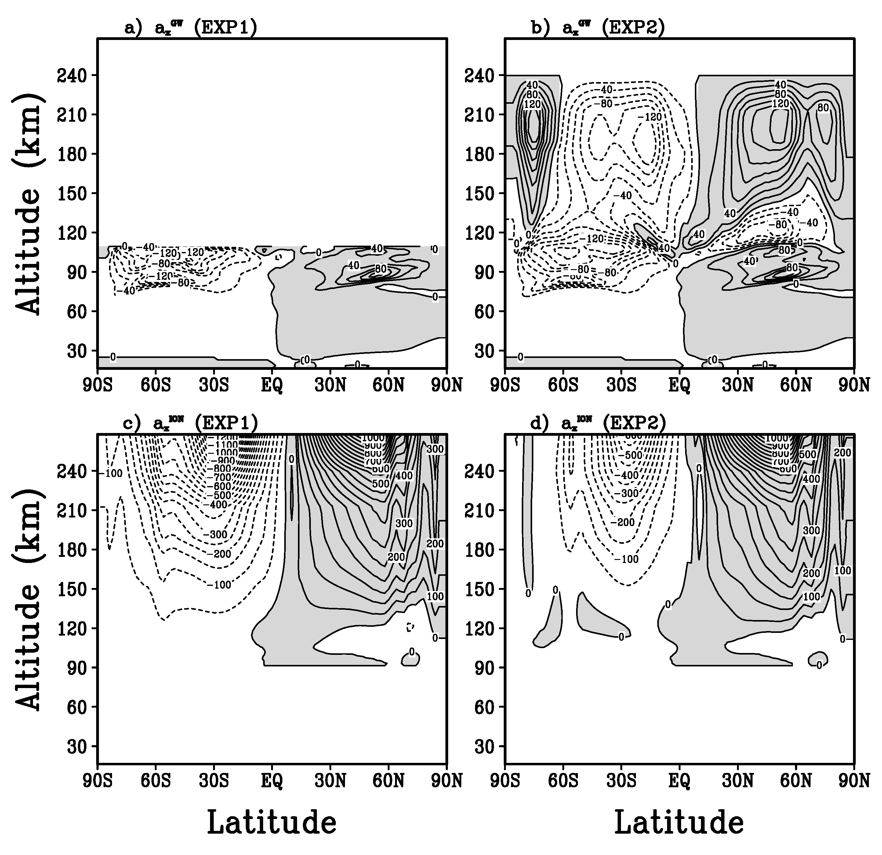
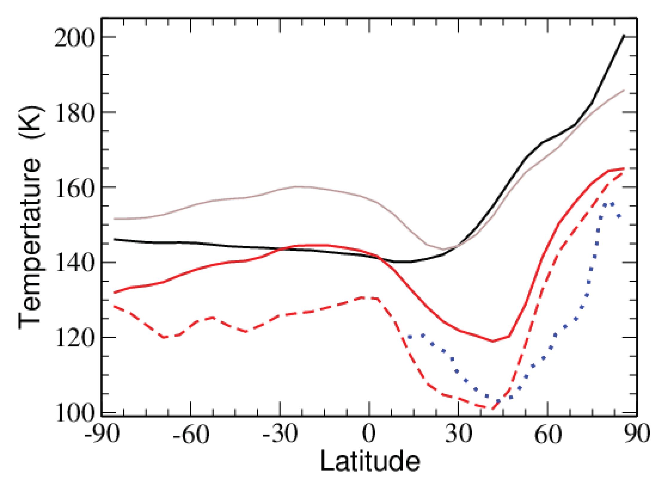
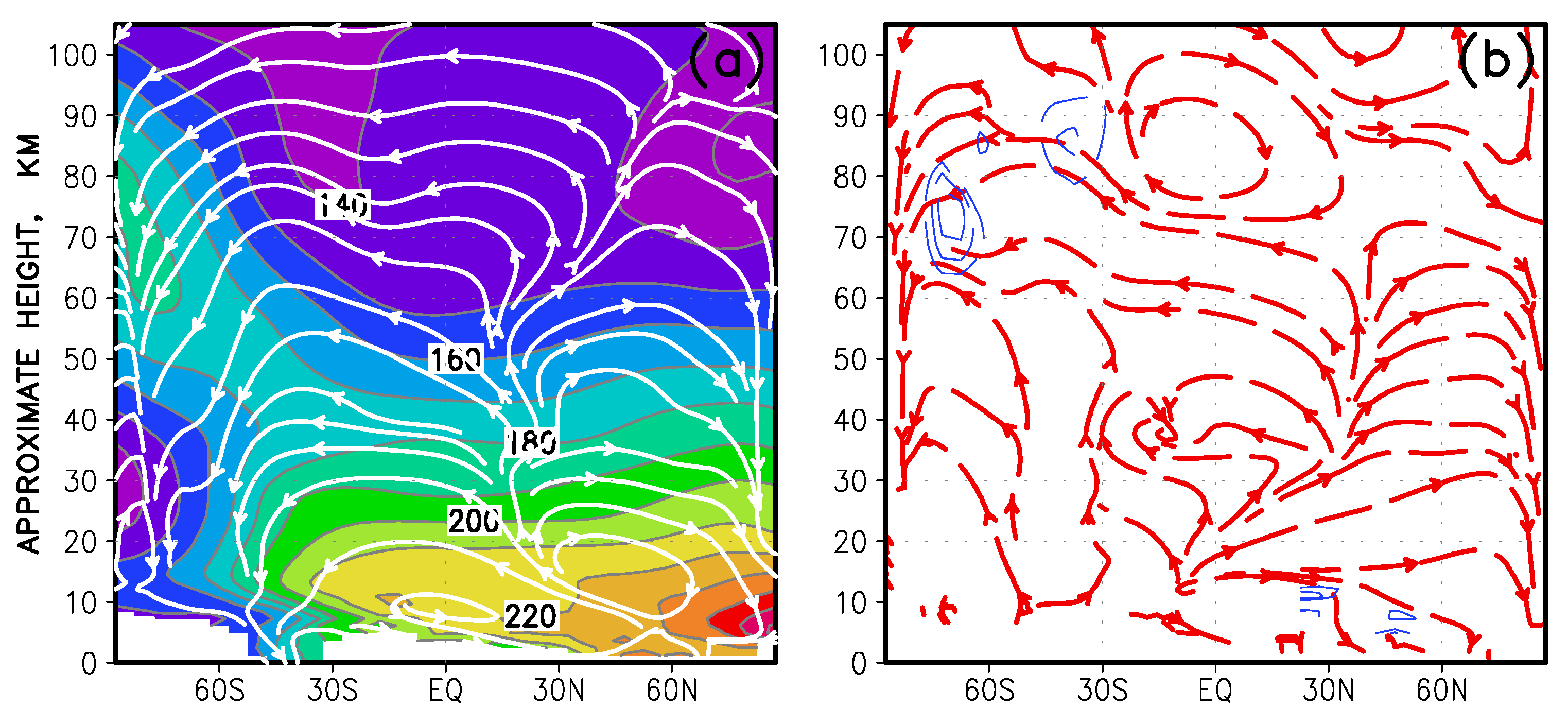
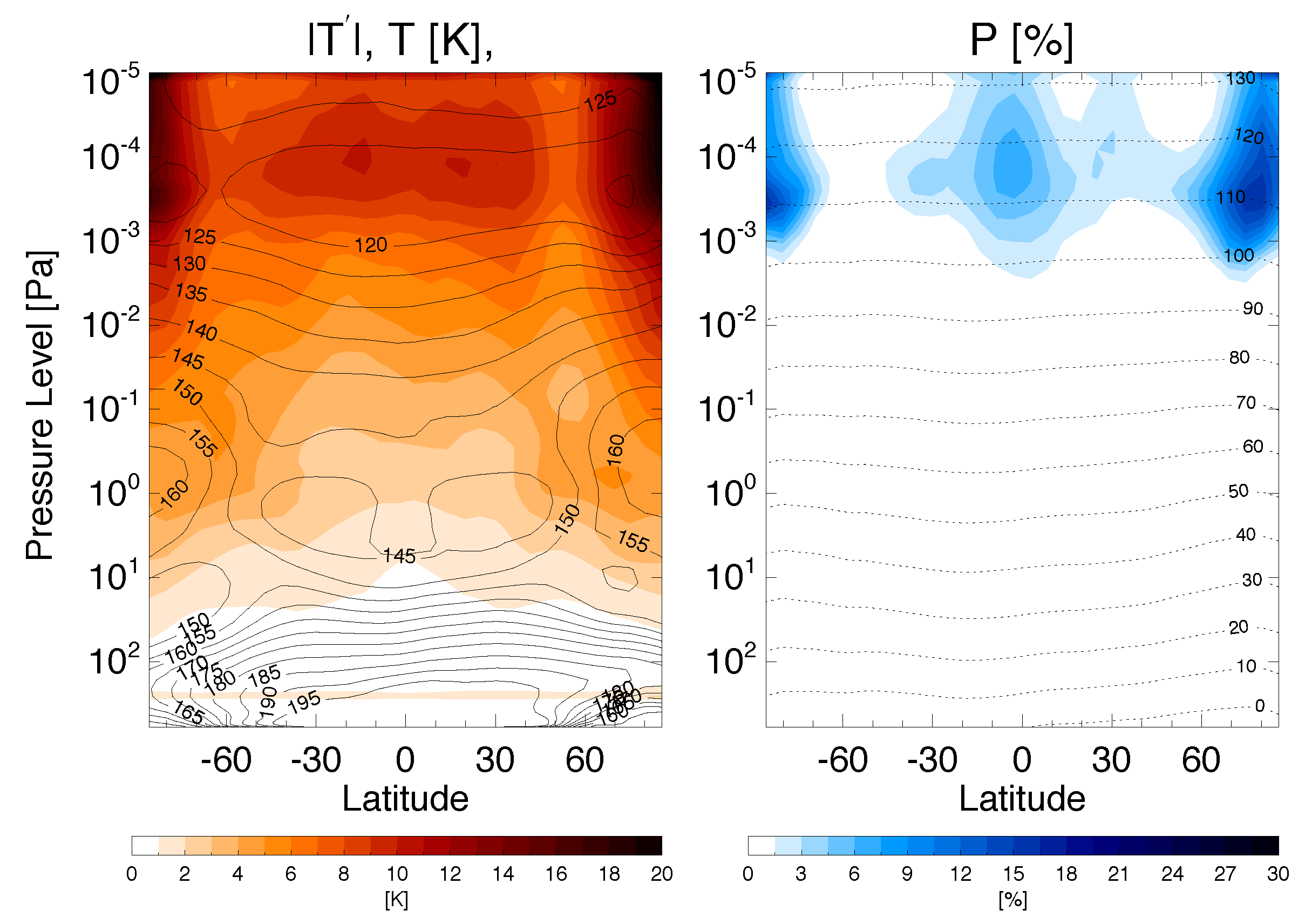
Table 1.
Characteristics of planetary atmospheres and expected maximal horizontal phase speeds of gravity waves. Jovian and Saturnian parameters are given for the stratospheric heights.
Table 1.
Characteristics of planetary atmospheres and expected maximal horizontal phase speeds of gravity waves. Jovian and Saturnian parameters are given for the stratospheric heights.
| Earth | Mars | Venus | Jupiter | Saturn | |
|---|---|---|---|---|---|
| Rotational frequency , s | 7.29 × 10 | 7.09 × 10 | 2.99 × 10 | 1.76 × 10 | 1.64 × 10 |
| Acceleration of gravity g, m s | 9.81 | 3.72 | 8.87 | 24.79 | 10.44 |
| Scale height H, km | 5.5–9 | 7.5–11.5 | 5–16 | 27 | 60 |
| Buoyancy frequency N, s | ∼2 × 10 | ∼2 × 10 | ∼2 × 10 | ∼2 × 10 | ∼2 × 10 |
| Max horizontal phase velocity, , m s | 220–360 | 300–460 | 200–640 | 1080 | 2400 |
© 2019 by the authors. Licensee MDPI, Basel, Switzerland. This article is an open access article distributed under the terms and conditions of the Creative Commons Attribution (CC BY) license (http://creativecommons.org/licenses/by/4.0/).
Share and Cite
MDPI and ACS Style
Medvedev, A.S.; Yiğit, E. Gravity Waves in Planetary Atmospheres: Their Effects and Parameterization in Global Circulation Models. Atmosphere 2019, 10, 531. https://doi.org/10.3390/atmos10090531
AMA Style
Medvedev AS, Yiğit E. Gravity Waves in Planetary Atmospheres: Their Effects and Parameterization in Global Circulation Models. Atmosphere. 2019; 10(9):531. https://doi.org/10.3390/atmos10090531
Chicago/Turabian StyleMedvedev, Alexander S., and Erdal Yiğit. 2019. "Gravity Waves in Planetary Atmospheres: Their Effects and Parameterization in Global Circulation Models" Atmosphere 10, no. 9: 531. https://doi.org/10.3390/atmos10090531
Note that from the first issue of 2016, this journal uses article numbers instead of page numbers. See further details here.