Recent Trends in Maintenance Costs for Façades Due to Air Pollution in the Oslo Quadrature, Norway


NILU-Norwegian Institute for Air Research, Instituttveien 18, Box 100, NO-2027 Kjeller, Norway
Atmosphere 2019, 10(9), 529; https://doi.org/10.3390/atmos10090529
Submission received: 6 August 2019
/
Accepted: 3 September 2019
/
Published: 8 September 2019
(This article belongs to the Special Issue Effects of Policy, Mitigation Measures and Economic Recession on Air Quality Trends)
Abstract
:This study assesses changes since 1980 in the maintenance cost of the façades of the historical 17th to 19th century buildings of the Oslo Quadrature, Norway, due to atmospheric chemical wear, including the influence of air pollution. Bottom up estimations by exposure–response functions for an SO2 dominated situation reported in the literature for 1979 and 1995 were compared with calculations for the present (2002–2014) multi-pollutant situation. The present maintenance cost, relative to the total façade area, due to atmospheric wear and soiling was found to be about 1.6 Euro/m2 per year. The exposure to local air pollution, mainly particulate matter and NOx gases, contributed to 0.6 Euro/m2 (38%), of which the cost due to wear of renderings was about 0.4 Euro/m2 (22%), that due to the cleaning of glass was 0.2 Euro/m2 (11%), and that due to wear of other façade materials was 0.07 Euro/m2 (5%). The maintenance cost due to the atmospheric wear was found to be about 3.5%, and that due to the local air pollution about 1.1% of the total municipal building maintenance costs. The present (2002–2014) maintenance costs, relative to the areas of the specific materials, due to atmospheric wear are probably the highest for painted steel surfaces, about 8–10 Euro/m2, then about 2 Euro/m2 for façade cleaning and the maintenance of rendering, and down to 0.3 Euro/m2 for the maintenance of copper roofs. These costs should be adjusted with the importance of the wear relative to other reasons for the façade maintenance.

1. Introduction
Air pollution and its impact on built structures has decreased in European urban areas during the latest decennia [1,2]. A question which is now more often raised, is whether the pollution remains a significant issue for the maintenance of building façades and windows. This paper discusses this question for the case of the Oslo Quadrature, Norway.
The first mainly wooden town of Oslo was built around year 1000, and burned down in 1624. The new city of Christiania was then built on the other side of the bay to the west, protected behind the Akershus castle. This city is today often the called “the Christiania Quadrature”, or, after the name of the city was changed in 1924, the “Oslo Quadrature”. Nearly all the buildings in the Oslo Quadrature have some protection status.
This work presents estimations of near present (years 1979 to 2014) trends and variation in maintenance and cleaning costs due to atmospheric wear, including the influence of air pollution, of the historic building façades in the Oslo Quadrature. The term “atmospheric wear” will be used in the following discussion for the chemical weathering, corrosion, and soiling processes on building façades. Of special interest was whether the maintenance costs due to the present local multi-pollutant situation are different from those reported in the literature for an assumed SO2 (sulfur dioxide) dominated situation in 1995. The costs were calculated by a so-called “bottom up” method, applying exposure response functions (ERFs), and represent situations when the atmospheric wear is the reason for the maintenance.
Since the beginning of modern industrialization, air pollution was observed to be an increasing health problem, and also to deteriorate and soil façades and built structures in industrial and urban areas [3,4]. From about the 1960s, it was realized that long-range transport of air pollution contributed to increasing overall pollution and acid rain [5]. The winds and weather transported acidic air pollutants to Norway from emission sources in the UK and European continent. The low alkaline buffer capacity in the Norwegian environment made the situation worse. Degrading effects of air pollution and acid rain on sensitive materials and cultural heritage monuments were reported and created an outcry [6]. However, one evaluation, of causes for the degradation of the stones of the Nidaros cathedral in Trondheim, concluded that after about 1990 the impact of air pollution on the church had been moderate as compared to other European locations, but added that the concentration and impact of SO2 was higher from before 1900 until about 1980 [7].
The observed accelerated atmospheric wear and damage to buildings and cultural heritage in Europe was caused mainly by acid rain and the deposition of SO2- and black carbon-containing particles [4]. From 1979 to 1995 there was a continuing decrease in the burning of sulfur-containing oil for residential heating in Oslo. Flue gas filtering of sulfuric emissions from industry, together with changes in the European industrial sector, associated especially with the large political and economic changes from about year 1990, contributed to the very significant reductions in SO2 emissions [1]. Today, the air pollution in European, and Norwegian, cities mostly comes from traffic and domestic heating. This change in emission sources has created a new air pollution mix, which is dominated by nitrogen oxides (NOx), particle matter pollution (PM), and, in some instances, tropospheric O3 (ozone). In some areas, mainly in Central and South Eastern Europe, annual mean concentration values of SO2 above 10 µg/m3 are still observed [1].
In the 1990s, the maintenance costs of façades in Europe due to local air pollution were estimated and reported in several bottom up studies. The pollution costs were derived from relationships between the observed damage on experimental samples chosen to represent façades, the assessed tolerable damage of façades before maintenance (the response), the pollution exposure, and the cost for the maintenance. The estimations were performed for both polluted and unpolluted, so called background, situations, to obtain results for the excess cost due to the local, for example, urban, air pollution [8,9,10]. The non-anthropogenic background pollution could be, for example sulfuric and particle emissions from volcanos, chloride-aerosol from sea-spray, and ozone from natural photolysis processes in the atmosphere [11]. Anthropogenic air pollution transported over a long-range to a wide area would also be included in the background pollution around a city. The distinction between the local and background pollution allowed the assessment of the separate impact and costs due to the locally emitted air pollution, which could be controlled by the local or national authorities, who would also experience the benefits. The emissions of the long-range transported pollutants were addressed by international negotiations and conventions [12]. Some studies also used a “top down” approach starting from records of the overall building renovation expenditures [13]. The costs were reported per square meter of building/monument surface per year (e.g., Euro/m2 per year), but also as cost/inhabitants per year (e.g., Euro/person per year), per concentration equivalent (e.g., Euro/person per year per µg/m3), and per emitted amount of the pollutant (e.g., Euro/kg SO2 or PM10 = concentration of particles with average aerodynamic diameter less than 10 µm). One overview of cost estimates of the damage to people’s health and built structures in Europe due to SO2 emissions [13] showed that the costs to the built structures were 1–4% of the health costs. A recent Swedish assessment found about similar costs (of about 1–6 Euro in villages and small towns, up to 60–80 Euro in large towns) per kilo emission of damages to health by exposure to PM10 from non-combustion road dust and of soiling of façades by total PM10 [14] (p. 91).
A bottom up study of maintenance costs of the façades of 17th to 19th century buildings in the Oslo Quadrature due to air pollution was performed in the end of the 1990s [15]. This study was based on exposure–response functions (ERFs) for materials and surface coatings, established through research in the EU-REACH [15,16] and ICP-materials projects (the International Co-operative Programme on Effects on Materials including Historic and Cultural Monuments, within the Convention on Long-range Transboundary Air Pollution, CLRTAP) [17]. These ERFs included the dominating impact of the dry deposition of SO2 together with the acid rain effect. The study compared estimates for the maintenance costs due to air pollution in 1979 and 1995, and calculated probable cost savings due to the reduction in air pollution over these years.
In the study by [15], it was found that the maintenance cost for a selection of façades facing the roads of the historical buildings in the Oslo Quadrature due to air pollution, including materials evaluated to be inert to air pollution, such as granite stone, had been reduced from about 1.7 Euro/m2 per year in 1979 to be about 1.4 Euro/m2 per year in 1995 (in 2019 prices). Of this, the cost due to the local air pollution (over background) was found to have been reduced from about 0.3 Euro/m2 per year (18%) in 1979 to only 0.05 Euro/m2 per year (about 4%) in 1995. These were even lower values than those found in other studies of European cities in the 1990s [13] (p. 152). The study by [15] concluded that from 1979 to 1995, the maintenance costs due to air pollution were reduced to low levels, barely over the background level.
In the situation from the 1990s, with a change in the air pollution mix in the urban atmosphere, an effort was made to establish a set of new ERFs to describe the possible deterioration impact on façades due to different air pollutants (other than SO2), and improve estimates for the atmospheric wear and costs in the “new multi-pollutant situation”. This work was carried out in the ICP-materials project and the associated EU projects Multi Assess [18] and CultStrat [19]. More focus was now given to the impact on cultural heritage, which was evaluated to be the more vulnerable part of the built environment. This work resulted in the establishment of ERFs for a smaller range of (four) different materials [20] and for the soiling of opaque surfaces [21] and glass [22,23]. The new ERFs facilitated more realistic assessments of the present maintenance costs due to air pollution, and comparison with the values and trends for the earlier years when the SO2 concentrations were higher.
Since the assessment of [15] for the year 1995, the assumption has mainly been that the local weathering and corrosion costs in Oslo are very low (insignificant), and that the long-range transport and background values of pollution and acid rain have decreased. This hypothesis, that the cost due to the atmospheric wear, including the influence of air pollution on buildings in the center of Oslo, remains low today, was tested in this work with new calculations by the ERFs for the multipollutant situation. Environmental data, which represent the recent situation in the Oslo Quadrature, were used. The results for the “present” multi-pollutant situation were compared with the costs in 1979 and 1995 reported by [15], calculated by ERFs for an SO2 dominated situation, and with the average costs for all the European ICP-materials stations [24,25].
Section 2 reports air pollution values and trends in the center of Oslo and its rural surroundings (the background). Section 3 gives the theoretical background for the understanding of the impact of air pollution on the deterioration of façades, their maintenance tolerances, practices, and costs. Section 4 describes the applied method for the bottom up calculations by ERFs of the recent atmospheric wear cost of the façades of the historical buildings in the Oslo Quadrature, and gives the input data for the environment in the center of Oslo, the façade materials, and their maintenance situations. Section 5 reports the results from the calculations. Section 6 discusses uncertainties and compares the estimated present (2002–2014) weathering costs with those reported for 1995 and with the typical total maintenance costs for municipal buildings in Norway.
2. The Recent Air Pollution Situation in the Oslo Quadrature and Rural Surroundings of Oslo
Measurements of air pollution started in Oslo at the end of the 1950s. The maximum concentrations were recorded in the first years of the 1960s, with about 400 µg/m3 SO2 and 150 µg/m3 “smoke” [26]. In 1979, the average annual concentration of SO2 in the inner city of Oslo was measured to be between 55 and 65 µg/m3 [27,28]. In 1995, it was measured to be below 10 µg/m3 everywhere in the city [15]. The background level of SO2 in the study by [15] was set to a concentration of 1 µg/m3. Figure 1 shows annual average concentration values of NO2 (nitrogen dioxide) and PM10 measured on air quality stations around the Oslo Quadrature, from 2003 to 2017 [29]. There was some decrease in values of PM10 and NO2 since year 2003, but with differences between stations and depending also on the introduction of new stations in the years from 2008 to 2010. It should be noted that the concentrations of PM10 and NO2 were probably somewhat higher in 1995 than in 2003, as can be seen for the station “Kirkeveien” in [30], and thus that some of the atmospheric wear on the façades in Oslo in 1995 should have been explained by the exposure to these pollutants.
Figure 2 shows pollution values measured since 1973 on the Norwegian EMEP (European Monitoring and Evaluation Programme) rural background station Birkenes in southern Norway [31].
Figure 2 shows a decreasing contribution from the long range transported and rural background pollution to the local air pollution in Oslo. The figures indicate a reduction in the contribution of the background pollution to the average atmospheric wear of façades in Oslo, and that calculations of the wear over the years from 2003 to 2014 could represent the present situation, in 2019, with a possible slight overestimation.
3. Theoretical
It is important that the method for the bottom up calculations by ERFs, of maintenance cost for the façades in the Oslo Quadrature due to atmospheric wear, represents the impact of the air pollution, the façade deterioration mechanisms, and the maintenance tolerances, practices, and costs in Oslo. The “maintenance tolerance” was defined here as the deteriorated, as compared to newly maintained, condition when the maintenance will typically take palace.
3.1. The Impact of Air Pollution
Building façades are exposed to particulate and gaseous pollutants by wet deposition in precipitation and dry deposition from air. Pollution deposited on the façade surfaces will generally increase the amount of adsorbed and absorbed water and the time of wetting. Pollutants that are dissolved in the surface water can react and deteriorate the façade material. Due to the consequent material loss, weakening, and other possible damages, maintenance will be needed. The ERFs applied in this work (Appendix A) describe uniform deterioration of façade surfaces due to multi-pollution deposition and reaction.
3.2. Façade Deterioration Mechanisms
Façades will undergo deterioration by mechanisms including combinations of physical, chemical, and biological processes. Air pollution is particularly involved in chemical deterioration. Uniform façade materials, such as metals and some stones, can deteriorate by slow, nearly even, thinning of the material. An oxidized corrosion patina develops on most metal surfaces. Over time (years), the corrosion will slow down to a constant rate with loss of metal through a patina layer of fixed thickness. The thinning of a uniform stone can happen by surface weathering and erosion, without much change in the surface characteristics, but patinas can form on stones too. The ERFs describe such uniform processes, which may be only the first phase of the atmospheric wear of the material surfaces. Patinas can be a protection, or they can change the degradation mechanism and accelerate the erosion, as in the well-known cases of the formation of voluminous porous and moisture-trapping rust layers on steel and black crusts on limestone, and subsequent exfoliation [8]. Many different processes, often related to water in its different phases and forms, and to environmental fluctuations, will contribute to the degradation of façade surfaces over their lifetime [32].
Many of the façades of the historical buildings in the Oslo Quadrature are covered with painted renderings. Paints applied on lime renderings were traditionally lime-based and permeable to the diffusion of water. Lime paints are recommended for application on renderings and would today mostly be used for the old buildings in the center of Oslo. The initial atmospheric weathering mechanism of such paints is similar to the underlying lime rendering, and resembles that of the limestone described by the ERF used in this work (Section 4.1 and Appendix A). Renderings and mortars consist of mainly carbonates, silicates, and alumina–silicates, mostly with calcium, and including solid fillers in different amounts, compositions, and grain sizes. The inert fillers, such as sand or ground limestone, increase the amount of material and improve the use, especially as mortars. Mortars typically contain a larger amount of filler material of larger particle sizes than the protective surface coatings of renderings. This improves the support and cementing of bricks and stones in walls [33].
The exposure of a lime-containing rendering or mortar surface to the air and its wetting will result in some amount of more or less uniform chemical dissolution, leaching, and weakening. The calcium carbonate (CaCO3) in the renderings and mortars is, as for limestone, susceptible to accelerated dissolution in a polluted and acidic environment. Physical expansion and contraction cycles due to wetting and drying, frost and thaw, pore crystallization and dissolution of salts, and temperature fluctuations contribute to the weakening and damage. Finally, the rendering or mortar cannot any longer hold together or stick to a substrate or other surface, and micro-cracks or crevices appear. This is a critical point in the deterioration. The cracking often happens at some non-uniformity in the surface. This can be due to, for example, variations in application thickness, geometric features, such as corners and angles, or solid inclusions, which are more important for mortars. Many different biological organisms, such as bacteria, fungi, lichens, mosses, and larger plants, can grow on and affect the deterioration process. Bio-growth can protect surfaces, but often contributes to their weakening and subsequent accelerated damage [34]. The breaking of the protective shell of a rendering or of the bonding of a mortar allows more access of the atmospheric influences to weaker points in the structure, with consequently more rapid leaching, weakening, and accelerated deterioration (Figure 3).
ERFs were used in this work to assess the material wear until the damage would be considered intolerable or the protective function of the material was compromised, and the resulting maintenance cost. For a rendering or mortar this is likely to be when some physical disintegration, such as cracking, appears in the material. In many cases, it is probably most cost efficient to do maintenance just before such physical damages appear. The mechanisms for the further deterioration, after the first damages to the rendering and/or mortar, would be very different for walls with painted lime rendering and limestone. The further deterioration of a compromised, e.g., cracked, material cannot be assessed with the ERFs.
Strong cements, other than those based on lime, and plastic-based paints, were used in Oslo from the second half of the 20th century. The resulting stiffness and non-permeability to water later created many problems. Problems have appeared due to non-compatibility of materials, the hindering of the natural hardening process in underlying lime mortars and renderings, and the trapping of water behind the paints. This accelerated deterioration happens mainly by physical processes, which are mostly unrelated to the slow deterioration of the solid cements and paints themselves [35]. The calculations of maintenance cost in this work do not represent such situations.
Materials, other than the metals and rendering, with a large presence in the buildings in the Oslo Quadrature are mainly wood, tile, brick, and glass. The deterioration of wood is usually mostly by biological wood rot and partly physical processes due to dimensional changes and cracking. Tiles, brick, and modern glass are relatively inert materials with slow deterioration. In general, such surfaces are more degraded by physical forces related to climate and water than by air pollution, and they could (as all types of façades) be damaged by the degradation of the supporting elements and the building structures. The atmospheric wear on these surfaces would mostly be by soiling, which could create a need for cleaning. Soiling due to air pollution is an accumulating process, which is represented by the ERFs applied in this work (Appendix A).
3.3. Maintenance Tolerances, Practices, and Costs
For the condition of a façade to be maintained, active intervention is needed at regular intervals. It was assumed in this work that the maintenance will take place when the wear of the façade surface has reached an intolerable extent, and that the aim is to preserve the physical condition over time. The wear would usually be intolerable when the integrity of the façade material is compromised and the degradation accelerates, for example, at the breakthrough of a metal sheet or surface coating. It could also be when the condition is considered unacceptable, such as for the soiling of windows. Accelerated wear or physical disintegration due to postponed or neglected maintenance, work faults, possible intentional changes to the façades, or perceptions of their (possibly changing) significance were not considered. Generally, with larger degrading influences from the environment more frequent maintenance is required. The maintenance cost of a façade due to atmospheric wear depends on the maintenance tolerance and the periodic maintenance cost.
No multi-pollutant ERF was available for renderings. The available ERF, for the weathering of Portland limestone, was therefore used for the renderings. It was assumed that the maintenance of a limestone rendering would happen when it had weakened to a condition where some small amount of physical damage had appeared, and that this condition could be represented by some uniform recession of a Portland limestone surface in the same atmosphere. This recession depth was set to 100 µm, suggested by [18] to cause deterioration needing maintenance of limestone ornament surfaces. Unfortunately, a direct experimental comparison of the degradation rates of lime-containing rendering and Portland limestone was not available.
It was assumed that the maintenance of a plain metal façade (zinc, carbon steel or copper) would happen after a period of atmospheric exposure, which caused certain a uniform recession similar to experimental metal samples. A galvanized layer on steel is typically 50 µm thick. The corrosion of this zinc layer would, however, not be uniform overall. The maintenance would generally happen when the galvanizing is broken through rather than fully corroded away. This would be at an average recession less than 50 µm. Values for the recession before maintenance, of 20 µm for the maintenance, and 30 µm for the replacement of the galvanized sheet, and 60 µm for the maintenance of the galvanized profiles, were used by [15]. The situation would be different for a zinc metal sheet and massive zinc used in, for example, monuments. A recession depth of 80 µm before maintenance of zinc monuments was suggested by [18]. In this work, recession depths of 20 µm and 80 µm before maintenance were applied, with the assumption that the situation would usually be in between. The corrosion rate of carbon steel is several times that of zinc [36]. Carbon steel used in building structures is nearly always galvanized and/or painted. Untreated carbon steel would seldom be used in situations of aesthetic importance. An untreated carbon steel surface rusts quickly and unevenly. However, due to its significant and predictable atmospheric corrosion response, carbon steel is often used as an experimental indicator material. For any usage the maintenance tolerance would, due to the higher corrosion rate, probably need to be larger than for zinc. No suggested value for the maintenance tolerance was available in the literature. A hypothetical maintenance tolerance of carbon steel surfaces of 200 µm recession was used in this work.
The time for cleaning interventions, and thus the cleaning costs for façades and windows, depends on the tolerated amount of soiling before cleaning. Cleaning practices will vary. It may be considered much more critical that frontal façades and windows, which should appeal to the public, are clean. The cleaning of, for example, rendered façades may be neglected until other more critical damages appear and overall maintenance or replacement is needed. The response to soiling could thus be different kinds of cleaning-maintenance operations.
The costs for maintenance work on façades varies depending on the kinds of surfaces and finishes. For example, the maintenance of cultural heritage façades with ornamentation would often require conservation specialists, at a much higher cost than if commercial companies could do the work with more standard procedures. The maintenance tolerance would affect the maintenance cost. With a low tolerance, the cost of repeated maintenance actions carried out more frequently and a delayed need for replacement of, for example, metal sheets or limestone renderings, could be less than for less frequent maintenance but earlier replacement.
The Discussion section will evaluate how the exposure situation, the materials, maintenance tolerances, and work costs of the façades in the Oslo Quadrature may be different from the model situation, and how that could affect the estimates for the maintenance cost due to atmospheric wear, including the influence of air pollution, which are reported in the Results section.
4. Methods
4.1. Exposure–Response Functions and Maintenance Cost Estimations
The estimations of maintenance costs due to atmospheric wear were made with available ERFs for a multi-pollutant situation. At moderate SO2 concentrations of 0–20 µg/m3, the ERFs for the multi-pollutant situation did not give significantly different results from those for the SO2 dominated situation, but explained more of the response by different, often local, air pollutants, like NO2 and PM10 [20]. The ERFs represented the atmospheric weathering-corrosion and soiling responses of a number of indicator materials, which could represent the façades in the Oslo Quadrature. The ERFs described the weathering of Portland limestone, representing lime renderings in this work, the corrosion of carbon steel and copper, and the soiling of white painted steel and modern glass in positions sheltered from rain and sunlight. The specific ERFs are given in Appendix A Equations (A1)–(A10). The general expression of the ERFs applied for the atmospheric corrosion and weathering Equations (A1)–(A4) is:
where R is the surface recession (m) of the material due to the environmental impact, P is the amount, usually the concentration in air (µg/m3), of some pollutant, n is the number of pollution terms, T (°C) is the temperature, H is the humidity, which can be given, for example, as the relative air humidity (%), Prec is the precipitation amount (usually in mm/year), pH is the acidity in the precipitation, and t (days or years) is the time of exposure with some order dependency, x or y.
The ERFs included a selection of the pollutant parameters: SO2, H+ (acidity in precipitation), PM10, NO2, O3, and Cl− (chloride), depending on the material. The expression for the pollution terms can vary from quite complex dependencies on the temperature and humidity to a simple linear dependence on time. Some different variations in the formulations were: the multiplication of the concentration terms for SO2 and O3 in the function for copper [20], the multiplication of the concentration values for NO2 and O3 to express nitric acid (HNO3), and the inclusion of the chloride concentration in rainwater in the last term in an equation for the corrosion of aluminium [15]. The time dependence was determined from four years of experimental exposures. In the cost calculations, extrapolation was usually made to longer lifetimes.
The total maintenance costs due to air pollution, Ct (Euro/m2 per year), the maintenance costs due to the background air pollution, Cb, and due to the local air pollution, Cp, were calculated from Equations (2)–(4):
where f (Euro/m2) is the cost of a maintenance or cleaning operation, and tt and tb (years) are the maintenance or cleaning intervals in the present ambient and background ambient atmospheres. tt and tb were calculated from the ERFs, from a defined maintenance tolerance (R), and the values for the environmental parameters in different air pollution situations. The estimations were made for the years 2002–2014, and could represent the “present” (year 2019). In accordance with the reporting of environmental data in the ICP-materials project, the reported years represented the start year for annual periods beginning in October that year and ending in October the next year.
The methods for calculating the costs by Equations (1)–(4) were described in more detail in [10,15,24,25,37]. In this work, the façade maintenance cost due to the atmospheric wear and soiling in Oslo were calculated for traffic, urban background, and rural background situations, from Equations (A1)–(A10) and Equations (2)–(4), using the environmental data given in Section 4.2. The “traffic situation” would typically be close to trafficked roads, whereas the “urban background situation” would typically be some distance away from such roads. The “rural background situation” would be outside of the city away from local pollution sources. The atmospheric wear costs for zinc were recalculated from [24]. The cost values for the soiling of white painted steel and modern glass were recalculated from [25]. “European averages”, calculated for all the stations with available data in the ICP-materials database for the years 1987–2014 [38,39], were reported to offer a simple comparison to the results for Oslo. The “European average” costs for carbon steel and copper were calculated in this work from Equations (A1) and (A2) and Equations (2)–(4). The “European averages” for Portland limestone and zinc were recalculated from [24], and for the cleaning from [25].
In addition, maintenance cost estimates made by ERFs for an SO2 dominated situation were presented for zinc (Equation (A11)), for the years 1987–2014, and for an inventory of ten different materials representing building façades in the Oslo Quadrature, for the years 1979 and 1995 [15]. The ERFs for the SO2 dominated situation included SO2 and H+, and in addition O3 for one material, copper.
The cost values for the inventory of façades in the Oslo Quadrature were recalculated from [15].
The recalculations were performed from values reported in the units of “% of one maintenance investment/year” and “Euro/m2 per year”, and partly as costs over background rather than the total and background costs reported here. Maintenance cost prices (Euro/m2) evaluated to be representative, or be a good basis for discussion, of façade maintenance costs in Oslo in 2019 (Table 1), were applied in the recalculations.
4.2. Façade Materials, Maintenance Situations, and Environmental Data
Figure 4 shows façades of historic buildings on and close to the main square of the Oslo Quadrature.
The painted renderings dominate the façades. Galvanized (zinc covered) steel surfaces and copper roofing are the main metallic surfaces. The estimated atmospheric wear and cleaning cost for the façades were described by the maintenance situations for the façades, as defined by the façade materials, the damage process (weathering/corrosion or soiling), the estimation year(s), the maintenance practices and costs, and the values for the environmental parameters needed to do the calculations by the ERFs, as given in Table 1 and Table 2. The tables are included here as summary references to the input parameters and values, which can be consulted as needed through the reading.
The values for the maintenance tolerances given in Table 1 were from the referenced literature and according to the description in Section 3.3. The values for the maintenance costs (Euro/m2) were obtained from the referenced literature and recalculated to 2019 prices by using the increase in labor cost in Norway of 155% from 1995 to 2019 [42]. The costs were based on reporting from different western European countries (France, England, Sweden, Czech Republic, and Norway) [13,14,41]. Cleaning is a relatively simple operation and the cleaning cost should be approximately correct for Oslo. The maintenance costs due to atmospheric wear will probably vary greatly between façades, buildings and work operations. It was decided to use the approximate average of European costs reported in the literature for a variation of single maintenance operations, of about 100 Euro/m2 [25]. However, this did not include costs for more complex maintenance with several consecutive work operations, including cost items such as the scaffolding, which would often be needed.
The values for the concentration of the air pollutants included in the ERFs (Annex A) were available from measurements performed at several air quality stations in Oslo, including one ICP-materials exposure station, which was the only station where pH in precipitation was measured. The approximate averages of the annual values of the pollutant concentrations measured at the stations around the center of Oslo were used in this work for the “T = traffic situation in the center of Oslo”. The average annual values for the pollutant concentrations measured at the ICP-materials urban background station in Oslo were used for the “UB = urban background situation in the center of Oslo”. A clearly significant difference in the pollution values in the urban traffic and the background situations was only observed for NO2 (Table 2). The averages of the annual values for the concentrations of the pollutants measured in the years from 2002 to 2014 at the rural background station Birkenes (Figure 2) in southern Norway were used for the “RB = rural background situation”. Chloride deposition was not measured at any of the stations. Considering that the Oslo Quadrature is located by the inner Oslo fjord, within one km from the shoreline, and that de-icing salts are used on roads in and around the city in the winter, a somewhat higher chloride deposition could be expected on the façades than in an inland natural background situation. However, the inner Oslo fjord is not a coastal location. The winds over the fjord are generally not much higher than inland and the waves and surf, which releases sea salt, are usually small. Most of the façades are, in addition, sheltered from the winds coming directly form the fjord by the terrain and other buildings. It was therefore decided to use a relatively low value for the chloride deposition, of 5 mg/m2 day. This would represent the approximate annual average sea salt deposition (of 2.5 mg/m2 day) some hundred meters from a coastline at low wind speeds (<3 m/s), considering also possible sheltering by trees and buildings [43] and a similar added amount of deposition from de-icing salt. The background value for the chloride deposition was set to zero to report a full measure for this “indicator for the chloride effect” on the carbon steel.
A significant part of the acidity measured today in southern Norway is still from long-range transboundary transport, which accounts for the lower value (of pH) reported in the ICP-materials database at the more southern location of station of Birkenes than Oslo [38,39]. The aim of this work was to assess the contribution of the air pollution in Oslo to the maintenance cost of the façades of buildings in the Oslo Quadrature, as compared to a rural situation outside of the city, without considering variations in long-range transport. There were no other measured values for acidity in rainwater available from stations closer to Oslo (than Birkenes). It was therefore decided to use a value of pH = 5.3 for the acidity in rainwater in the rural background (in the rural area close to the city), as compared to the value of pH = 4.7 which was measured at the Oslo ICP-materials urban background station, and the value of pH = 5.0 which was measured at the Birkenes station, as the average of the five years of measurement from year 2002 to 2014 [38,39]. The annual average values for the climate (temperature, precipitation amount, and relative humidity), measured at the central Oslo meteorological station at Blindern from year 2002 to 2014 and reported to ICP-materials [38,39], were used in all the calculations.
5. Results
Figure 5 shows the results for the estimation of the maintenance and cleaning costs of the building façades in the Oslo Quadrature in the years from 1979 to 2014 due to atmospheric wear, including the influence of air pollution. The figure includes a complete comparison of the calculated costs by the ERFs for the noted, and differently colored (in text and outline), materials and pollution situations over the evaluation years. The initial impression of the figure may be somewhat confusing, but every displayed point (on the curves) is simply the calculated maintenance cost for one material in one year in one of the pollution situations given by the legend and colored text. Thus, each legend entry in grey represents all the similarly outlined curves of different color. The main purpose of the figure is to compare the values for the SO2 dominated situation in 1979 and 1995 and for zinc since 1987 with those estimated for Portland limestone, carbon steel, copper, and for the cleaning of white painted surfaces and glass, for the multi-pollutant situation, from 2002 to 2014. For Portland limestone, carbon steel, and the cleaning there were no observable trends in the results in the multi-pollutant situation, but significant variation between the years. For the sake of presentation and comparison, it was therefore decided to show the average periodic costs (straight horizontal lines) from 2002 to 2014 for each of these materials.
The upper part of Figure 5A compares the values in 1979 and 1995 with maintenance due to weathering-corrosion. The lower part of Figure 5B compares the same values in 1979 and 1995 with cleaning costs due to soiling and haze. By the legend and colored text, Figure 5 gives the main conditions for the estimations related to the pollution situations (traffic, urban, and rural background situations) and the maintenance tolerances (R) applied in the estimations for the many materials. The display of all the results in the two connected diagrams, Figure 5A,B gives a quick impression of how the values for the maintenance cost estimates for the “present” (2002–2014) period compare to the recent past (1979–1995). As the single materials were not directly comparable, except for galvanized sheet and zinc, this seemed to be the best way to give an overall comparative view of the estimated maintenance costs and trends. The crosses on the curves show the measurement/estimation years. For simplicity, Figure 5B only shows the lowest and highest maintenance costs calculated for individual materials in 1979 and 1995. The “European average” costs for copper were similar to the values in the center of Oslo and are not shown.
The main result seen in Figure 5A is that the present (2002–2014) estimated maintenance costs due to atmospheric wear are in the same overall range as from 1979 to 1995. The estimated maintenance cost of painted steel in 1995 due to atmospheric wear, shown in Figure 5, was about four times higher than for any other material. As an ERF for the multi-pollutant situation did not exist for painted steel, no calculation was made for this material for the 2002–2014 period. Considering, however, the relative similarity of the cost estimates for other materials since 1979, the situation, with much higher cost for the maintenance of the painted steel, would probably be similar for the years after 1995. The maintenance cost due to air pollution after 2002 for metallic surfaces (zinc, copper, and carbon steel, without including a chloride effect) remains low with an impact of the local air pollution, which seems only very slightly above that of the rural background pollution for these materials. At the lower maintenance tolerance for zinc, of 0.2 mm recession, and when the very significant chloride effect was included for the carbon steel, the present (2002–2014) maintenance costs were estimated to be two to three times that of the most relevant single façade material, galvanized steel, in 1995. The present maintenance cost for Portland limestone (see Discussion), which could represent lime renderings, was estimated to be significantly higher than in 1995, but still much lower than for painted steel.
Figure 5B shows that the cleaning cost, especially for glass/windows, may today generally be higher than the corrosion costs (Figure 5A, see also Discussion). Except for the much higher values calculated for the carbon steel corrosion for the European ICP-materials averages, the cost values for these averages were about similar to the values for Oslo, as is also shown by comparison to values reported in [25]. The reason for the lower steel corrosion in Oslo is the sensitivity of carbon steel to SO2 and the lower measured SO2 concentration in Oslo (Table 1, [38,39]). Contrary to the large variation between years in the cost values for the single station in Oslo, the European ICP-materials averages indicate a trend towards lower maintenance costs due to atmospheric wear of façades over the period 2002 to 2014.
Figure 5 further shows higher estimated cost over background for the maintenance of Portland limestone (Figure 5A) and cleaning of soiled surfaces (Figure 5B) in the multi-pollutant situation than for any material in the SO2 dominated situation in 1995. Table 3 and Table 4 in the Discussion section give the cost values for 1979, 1995, and averages from 2002 to 2014, shown in Figure 5.
6. Discussion—Uncertainties
Some aspects related to the impact of the air pollution on experimental samples and façades, and the measures for the maintenance costs, will be discussed. The present (2002–2014) maintenance costs due to the atmospheric wear will then be compared with the costs in 1995 and with the total building maintenance cost.
6.1. The Impact of Air Pollution on Experimental Samples
The applied ERFs represent the average of the measured atmospheric impact on material samples at a selection of European exposure stations. It is worth investigating how the situation in Oslo is represented by this average. Figure 6 shows the responses by the ERFs calculated from the environmental values measured at the Oslo ICP-materials urban background station, and the respective measured first year surface wear of experimental samples at the station. Results from the ERF for the soiling of white painted steel Equation (A5) are not shown in Figure 6, as data from Oslo were not used in the development of this ERF. This ERF was developed in the 1990s based on exposures in European cities with high air pollution: London in the UK, Katowice in Poland, and Athens in Greece [21].
The results for the multi-pollutant ERFs are only shown from 2002, as PM10 values for Oslo were only available from that year, based on correlation with particle deposition [22]. The same ERF for zinc in an SO2 dominated situation was used for all the years. As the ERFs were developed by statistical methods from measured environmental and corrosion data, some differences between the calculated and the measured values for the wear at single stations is expected. This difference is an indication of how well the ERFs represent the observed situation at that station. Figure 6 shows that for Oslo there was no systematic error in the wear calculated by the ERF for Portland limestone, but significant uncertainty in the prediction for single years. The zinc function systematically underestimated the loss of glass-blasted zinc exposed from 2002 to 2014, but not in the years 1997 and 2000, and overestimated that of ground samples, except in 1987 and 1992. The carbon steel and haze functions overestimated the responses measured on these materials.
The zinc function was developed for ground zinc in the SO2 dominated situation. Glass-blasted zinc has a somewhat rougher surface and higher corrosion rate, as can be seen for the years 2000 and 2008, when the corrosion of these different surface finishes was compared experimentally [36]. The larger presence of different pollutants relative to SO2 after 2000 may be another reason for the underestimation of the corrosion of glass-blasted zinc from 2002. A new multi-pollutant function was developed for zinc [20], but more recent correlations within ICP-materials [44] indicate that this inclusion of additional pollutant terms is uncertain.
Metals are, generally, sensitive to chloride corrosion. This is important for, for example, painted steel surfaces. When damages appear in the paint film the degradation will happen much more quickly in a chloride containing environment. Chloride deposited on stone façades can increase the erosion caused by salt crystallization and dissolution. Chloride was not included in the ERFs used in Figure 6. The corrosion of carbon steel, which is the metal most sensitive chloride exposure, was overestimated. This shows that the chloride effect in the urban background in Oslo is probably small. De-icing salts are used on many roads in Oslo during the winter, and the exposure of façades and wear due to exposure to de-icing salts could still be significant in some situations.
The overestimation for carbon steel could be due to longer periods of cold and dry weather in Oslo giving less corrosion than the European average, and/or differences in the composition of PM10 in Oslo as compared to other ICP-materials locations. Oslo has several winter months during the year with temperatures below freezing and snow. This may reduce the corrosion of metals as compared to the European average, but could possibly increase the physical erosion of stones and other materials, related to frost, thaw, and humidity cycles. PM10 consists of a range of possible particle sizes and compositions, which will vary between locations, and which could have different corrosion effects. Oslo has substantial emissions of fine particles from residential wood burning on cold winter days and of re-suspended road dust on days with dry and cold weather in the winter and spring. This emission often happens together with temperature inversions, which traps the pollutants in stable air over the city and gives the highest concentrations of PM10 though the year. It may be that the exposure to this PM10 in Oslo is relatively less corrosive and soiling than the average European PM10 exposure.
The ERF for the soiling of white painted steel only correlates the soiling with the PM10 concentration and the experimental correlations were rough [21]. Climate factors were not included. This was expected to give more uncertainty in calculations by this ERF. The fraction of black soot from diesel engines and industry in the measured PM10 was probably a major reason for the observed experimental soiling. PM10 in Oslo is probably different from a theoretical European average, and contains less black carbon than the experimental situations, in Athens, London, and Prague, in the 1990s.
The comparisons in Figure 6 show that the maintenance costs reported in Figure 5 for the carbon steel without chloride exposure and the cleaning of glass were probably overestimated, with a factor of about two. If this is due to less impact of PM10 in Oslo, then the cleaning costs for the white painted steel in Figure 5 were probably also overestimated.
6.2. Comparison of Atmospheric Wear on Experimental and Façade Materials and Measures of Maintenance Costs
The applied ERFs represent a selection of façade materials. It is worth questioning whether the sample materials represent the façade materials over their lifetimes and how the mainly uniform measured weathering on the sample materials represents the variation in the weathering on the façades in the Oslo Quadrature.
There will be variations in weathering depending on the exposure orientation of façades. The experimental metal samples were exposed in open exposure at 45 degrees to the horizontal. The limestone samples were exposed vertically in open exposure. The glass samples were exposed vertically and sheltered from rain and sunlight. As roofs are more commonly made from metal sheet, whereas renderings and glass are usually applied on walls, the experimental sample orientation should represent the façades.
The atmospheric wear of uniform façade material, like bare metals (zinc and carbon steel) and probably also brick and tile, will probably be quite similar to experimental samples. Still, the surfaces of, for example, the galvanized zinc façades in the Oslo Quadrature would be different from glass blasted and ground zinc, and their corrosion could be systematically different from the experimental samples. Based only on the difference between the glass blasted and ground zinc samples, and assuming that the first-year corrosion of the galvanized façades was in the same range, the uncertainty in the maintenance cost estimates for the zinc façades could be in the range of about −75 to +100% of the reported values. However, this uncertainty was not very important for the overall cost evaluation, as the present estimated maintenance costs of zinc façades in Oslo due to the atmospheric wear were low. This variation does, however, indicate significant general uncertainty in the reported cost estimates, depending on the surface properties. The extrapolation by the ERFs to longer lifetimes than in the experimental exposures (four years) gives additional uncertainty.
An ERF for the weathering of Portland limestone was used to indicate the maintenance costs for limestone renderings, which are significantly different from Portland limestone. It was assumed that the chemical mechanism which weakens the rendering until it cracks was similar to the weathering of limestone, and that a certain leaching of the limestone could represent the “cracking point” for the rendering. The cracking point was set to 0.1 mm uniform leaching of a Portland limestone surface. Although the initial weathering processes and leaching of limestone and lime renderings have similarities, the application of this maintenance tolerance for limestone ornaments (of 0.1 mm) to lime renderings is clearly uncertain. The relatively high maintenance cost for Portland limestone shown in Figure 5 is an indication and warning about the sensitivity of the renderings. The mechanism for the degradation of Portland limestone versus renderings is, however, not sufficiently understood to give a precise evaluation. The cleaning of façades with rendering may be less relevant than atmospheric weathering, as the replacement of renderings would probably often be the single maintenance response. In the possible case of cleaning of the non-white façades of the historic buildings, the tolerance for soiling before cleaning may be higher, and the cleaning cost due to the atmospheric impact then lower, than that shown for the white painted façades in Figure 5. Thus, the evidence is not sufficient to conclude that the atmospheric wear costs for the lime renderings were different in the multi-pollutant situation from 2002 to 2014 than they were in 1995.
The variation in the weathering on the larger and more complex surfaces of buildings will generally be larger than on smaller samples, which may lead to different wear characteristics and maintenance responses. Such local variations are not considered in the estimations with the ERFs. The starting point for any particular evaluation of damage would usually be understand if the degraded part of a façade or other element was in some way differently exposed to higher environmental loads or other damaging influences. For example, there would be local variations in the concentrations of NO2 and PM10 depending on such factors as the distance from the traffic, the form of the street canyons, and local emissions from residential wood burning. The sheltering of different parts of the façades could significantly affect the weathering. Areas sheltered from rain can be subject to more degradation due to dry deposition and the accumulation of corroding pollutants, whereas non-sheltered areas may be more affected by rain wetting and washing. The experimental exposure situation of the modern glass samples was clearly different from that of most ordinary windows, which are usually exposed to some rain-washing. What the impact of rain-washing is on the observed haze on windows as compared to the calculations by the ERF, and on the perception about needed cleaning, seems to be not well known. Quicker than average wear on critical points of a construction may lead to local repairs and an earlier need for general maintenance than expected from the average corrosion and weathering. It may be difficult to assess how this could affect the overall maintenance cost, but it would probably be towards higher costs.
It is worth questioning what the maintenance costs for the façades, as given in Table 1, represent and how correct they are for the year 2019. The maintenance work on façades will usually consist of several steps, such as diagnosis, cleaning, repair, consolidation, and protection. In some cases, the maintenance could be considered a one step process, such as for façade and window cleaning. In other instances, façade cleaning would be the first step before further maintenance actions. The extensive conservation of more complex ornamented façades or monuments could include more steps and different processes and be very expensive. The maintenance cost due to the atmospheric wear reported in this work indicates the expected cost for relatively simple one-stage maintenance operations. For complex maintenance operations the cost would probably be higher.
This discussion shows the many challenges with comparison between weathering and soiling of experimental samples and façades with variations in material properties and degradation rates, and in determining the condition and costs for maintaining them. The cost due to atmospheric wear of façades, including the influence of air pollution, that was reported in this work should therefore be considered indications of the costs. They are suited to reporting trends. The absolute values are more uncertain. The uncertainty represented by the different single input parameters to the cost estimations by the ERFs should be evaluated in each concrete case. It may be wise to make calculations for a range of maintenance tolerances and report a range of costs, as for zinc in Figure 5.
Lastly, it is important to note that façades are often maintained for reasons other than the atmospheric chemical and microphysical wear, and soiling, which was estimated by the ERFs applied in this work. The atmospheric wear may be the major reason for the maintenance of façades in some situations, for example, along trafficked roads. Other reasons for façade maintenance may be different degradation processes affecting the building and the façades, such as various physical processes related to water exposure and penetration, cracking due to structural movements and loads, vandalism, or even changes in aesthetic perceptions unrelated to the physical condition. The degradation will usually happen by a combination of mechanisms. The relative importance of the atmospheric wear for the maintenance could vary between 0 (uniform atmospheric wear, including the influence of air pollution, is not important) and 1 (uniform atmospheric wear, including the influence of air pollution, determines the cost). Even if it can be difficult to determine the relative importance of degradation processes, the value of this factor could be suggested by performing case specific condition evaluations and studies of the decision processes leading to the maintenance actions. However, such analyses were beyond the scope of this work.
6.3. Comparison of Cost in 1995 and 2019
Table 3 shows the materials inventory from the study by [15], of the façades facing the street in the Oslo Quadrature, of eight buildings from between 1626 and 1800, and another eight buildings from between 1800 and 1914. The table gives an impression of the types and relative amounts of surface materials of façades from before 1914, even if the inventory clearly depends on the selection of the buildings. If, for example, the building in Figure 4b had been included (the buildings in Figure 4a,c were included), then a larger surface area of brick would have been in the inventory.
Table 4 shows the calculated maintenance costs due to atmospheric wear in the multi-pollution situation in the period 2002–2014, in 2019 prices.
The cleaning cost of glass and carbon steel in 2002–2014 was adjusted to half the value shown in Figure 5, the atmospheric wear cost of renderings, as represented by Portland limestone, was assumed to be similar to the cost for rendering in 1995, and it was considered that the cost for possible façade cleaning could probably be represented by the average cost found for maintenance of the façade materials, all in accordance with the discussion in Section 6.1. The background costs were adjusted similarly. The addition of the costs for the window cleaning increased the atmospheric wear cost of the historical façades in the Oslo Quadrature by about 15%, from 1.4 Euro/m2 per year, calculated by the SO2 dominated ERFs in 1995 (Table 3), to 1.6 Euro/m2 per year, calculated for the present multi-pollutant situation (2002–2014) (Table 4). Clearly, they cleaned windows in 1995 too, and this approximate cost could have been included in the total for 1995.
The cost due to the local air pollution was estimated to be a significantly larger part of the total maintenance cost due to the atmospheric load and wear of some materials in 2002–2014 than in 1995. When including the window cleaning in the 2002–2014 period, the maintenance cost due to the local air pollution increased to about 15% (0.26 Euro/m2 per year) of the total cost, as compared to 5% (0.07 Euro/m2 per year) without the window cleaning and in 1995. When including the adjusted value for the Portland limestone as a substitute for maintenance of the 50% of the façade area with renderings, the cost due to the local air pollution increased to about 40% (0.62 Euro/m2 per year) (Table 4). This significant difference between the reported values for 1995 and those calculated for the present (2002–2014) was due to the experimentally observed degrading influences of NOx gases and particulate air pollution (PM10).
6.4. Comparison with Total Building Maintenance Cost
The total costs for maintenance, including technical installations of public buildings in Norwegian municipalities, have been reported to be in the range from 90 to 115 NOK/m2 gross floor area [45]. With an increase in work cost of about 40% since the reporting year 2004 [42], the approximate maintenance cost in 2019 would be 140 NOK, or about 15 Euro/m2 floor area. Assuming three story buildings in the inventory from [15] (see Figure 4) of 10 m height with an average depth from the street of 10 m [46], the total square meter gross floor area would be: the total façade area of 19,058 m2 times three, equals 57,174 m2 (= the façade area (19,058 m2) / façade height (10 m) × Building depth (10 m) × 3 floors). The total present (2002–2014) overall atmospheric weathering cost, including the influence of air pollution, was estimated to be about 1.6 (1.62) Euro/m2 façade per year (Table 4). Assuming no change in the atmospheric loads since the period 2002–2014, the maintenance cost due to the atmospheric wear, including air pollution, in 2019 would be about 3.5% (1.62 × 19,058)/(15 × 57,174) of the total maintenance costs, which would amount to about 30,000 Euro/year (15 × 57,174 × 0.035%) for the 16 buildings. The local air pollution was estimated to account for 38% of this, or about 1.3% (0.38 × 3.5%) of the total maintenance cost, equal to about 11,150 Euro/year (15 × 57,174 × 0.013%). It may be that the maintenance costs for the façades, including the required preparations and multiple work operations, are higher than the 100 Euro/m2 façade per year assumed in this estimation (Table 1). On the other hand, the total maintenance cost may be higher for these protected buildings than the 100 Euro/m2 gross floor area per year reported for the typical municipal buildings. Some part of the cost would be due to different deterioration or evaluations than those related to the atmospheric façade wear. There are surely differences between cases and variations in costs. Separate cases could be evaluated with more precision based on detailed observations of the extents, causes, and reported reasons for the deterioration and maintenance operations, including the work costs.
Possible adjustment (AV) of the reported values (RV), of maintenance cost for the façades in the Oslo Quadrature due to the present atmospheric wear, including the influence of air pollution (Table 4), could be made for different work costs and the relative importance for the maintenance of the atmospheric wear, by the following calculation:
Adjusted value (AV) = RV × the observed maintenance work cost relative to that used here in Table 1 × the factor relevance of uniform atmospheric wear (between 0 and 1). The percentage cost for the atmospheric wear relative to the total maintenance cost per m2 gross floor area could then be easily recalculated by replacing the value of 15 Euro/m2 gross floor area used in the calculation: AV/(15 × 3), with a corrected total cost (different from 15 Euro). For different maintenance tolerances, a recalculation by the ERFs would be needed.
7. Conclusions
The main conclusions from this study of maintenance cost due to atmospheric wear and soiling of the façades of the historic buildings in the Oslo Quadrature, including the influence of air pollution, are distinguished by four points below, about: (1) maintenance cost due to atmospheric wear and soiling for the total façade area and compared to the total maintenance costs for the buildings; (2) the maintenance cost due to atmospheric wear and soiling of single façade materials; (3) the effect of chloride exposure on the façade maintenance costs; (4) the variation in façade maintenance costs for single façade materials and associated uncertainty in the estimations. Lastly, the concluding paragraph gives an overall evaluation of the importance of multi-pollutant exposure situation for the present and future maintenance cost for the façades in the center of Oslo.
- The total maintenance cost due to atmospheric wear and soiling in the present multi-pollutant situation is about 1.6 Euro/m2 per year, with the local air pollution costing about 0.6 Euro/m2 total façade area per year, or 40% (38%). Of this local air pollution cost, the cost due to wear of renderings is about 0.4 Euro/m2 per year (22%), cost due to the cleaning of glass about 0.2 Euro/m2 per year (11%), and cost due to wear of the other façade materials about 0.07 Euro/m2 per year (5%). The maintenance cost due to the atmospheric wear was found to be about 3.5%, and that due to the local air pollution 1.3%, of the total maintenance costs for the buildings, including their technical installations, which would amount to about 30,000 and 11,150 Euro/year for the 16 buildings;
- The present (2002–2014) maintenance cost per square meter of specific façade material due to atmospheric wear, including the influence of air pollution, is probably highest for painted steel surfaces, about 8–10 Euro/m2 per year. Among the other façade materials, this cost was indicated to be highest for lime renderings, about 3.1 Euro/m2 per year. The uncertainty in this estimate was large, due to the applied comparison with Portland limestone, so a difference from the cost of 1.9 Euro/m2 per year found in 1995 could not be determined. The costs for the cleaning of sheltered modern glass were evaluated to be about 2 Euro/m2 per year and of the other façade surfaces about 1.6 Euro/m2 per year. This takes into account that the soiling impact of PM10 in Oslo seems to be less than for the average of European experimental locations. The cleaning costs would clearly vary depending on the local exposure situations, as in trafficked roads, backyards, or the urban background. For renderings and painted façades it should be considered if maintenance actions other than cleaning, for example, replacement and repainting, could be the response to the wear. The maintenance costs for metallic surfaces (zinc, carbon steel, and copper) due to air pollution, excepting possible exposure to chloride, were found to be similar to those reported for 1995, below about 1 Euro/m2 per year, with the lowest cost for copper, of about 0.25 Euro/m2 per year. A possibly slight continuing trend of reductions in the maintenance costs for the metallic surfaces since 1995 was indicated;
- The estimations showed a significant possible effect of chloride exposure, which could increase the cost for the maintenance of carbon steel surfaces in the center of Oslo from about 0.25 to 2 Euro/m2 per year. No such chloride impact was measured on experimental samples on an urban background station in Oslo, which indicates that the wear from sea salt chloride of the façades in the Oslo Quadrature is probably small. However, local exposure to de-icing salts could significantly increase maintenance costs;
- It was found that the variation in the maintenance cost due to atmospheric wear, depending on the type of zinc surfaces and their maintenance tolerance, might be on the level of a possible chloride effect, of about 2 Euro/m2 per year with an uncertainty of about −75 to +100%. This is an indication of general uncertainty of the cost estimates, depending on variations in surface properties of the façade materials. Other differences between experimental samples and façade materials and changes during the lifetimes of the façades could give additional uncertainty.
The results indicate that the present (2002–2014) multi-polluted urban atmosphere in the center of Oslo is a significant contributor to the total maintenance cost for historic façades. This is especially so for sensitive surfaces with low cleaning/maintenance tolerances, such as glass and façades which are easily soiled, lime-containing renderings and mortars, and fine stonework and ornamentation. For metallic surfaces, the contribution of local air pollution to the maintenance need and costs has been very small to insignificant since 1995. The main reason for the remaining influence of air pollution is the still significant emissions of particulate matter and NOx gases. Thus, some savings in the maintenance cost for façades could still be obtained by reducing these emissions. The future will show how opposite trends, like the significant electrification of the vehicles and the rapid urban development and growth in Oslo, will affect the local air pollution values and impacts.
Author Contributions
The author (T.G.) have had long duration engagement with the ICP-materials project (http://www.corr-institute.se/icp-materials) within which measurements of the atmospheric wear and soiling of experimental materials, and of environmental parameters took place, and where the basis for the cost assessments methodology was developed. The author have the full responsibility for the application of these data and the methodology in this work. Conceptualization, methodology, validation, formal analysis, investigation, resources, data curation, writing—original draft preparation, writing—review and editing, visualization, supervision, project administration and funding acquisition: T.G.
Funding
This research was performed with support from the Norwegian Environment Agency, to NILU-Norwegian Institute for Air Research as partner in ICP-materials, and from NILU.
Acknowledgments
The basis for this work is the 30 years of field work, analysis and reporting by the partners in the International Co-operative Programme on Effects on Materials, including Historic and Cultural Monuments (ICP-materials). The ICP-materials programme was started in 1985 to provide a scientific basis for protocols and regulations to be developed within the Convention on Long-range Transboundary Air Pollution under the United Nations Economic Commission for Europe (UNECE). The author thanks all present and past ICP-materials partners for their invaluable work over all these years, which today make works like this possible.
Conflicts of Interest
The authors declare no conflict of interest.
Appendix A
This appendix contains the formulations of the exposure–response functions (ERFs) which were applied in the calculations in this work.
For the multi-pollutant situation, the following ERFs were applied.
For the recession of carbon steel, [20]:
where RH60 = (Rh − 60) when Rh > 60, otherwise 0, and f(T) = 0.15(T − 10) when T < 10 °C, otherwise −0.054(T − 10). The part for the chloride contribution was added based on the description in [47] (p. 127).
For the recession of copper, [20]:
where RH60 = (Rh − 60) when Rh > 60, otherwise 0, and f(T) = 0.15(T − 10) when T < 10 °C, otherwise −0.054(T − 10).
For the recession of Portland limestone [20]:
where [HNO3] can be approximated by [25]:
For the soiling of sheltered white painted steel [21,40]:
where ΔR is the loss of reflectance (%) relative to the reflectance of the non-soiled surface, R0 (%) at time zero, [PM10] is the concentration of PM10 (particles with aerodynamic diameter ≤ 10 µm) in µg/m3, and t the time of exposure (days). The constant (=3.96 × 10⁻⁶) then have the unit m3/µg × t.
For the soiling of modern glass, the average of the result calculated with equations for the haze development on sheltered modern glass was used, as reported by [22]:
and by [23]:
In the Equations (A6), (A9) and (A10), t is the time (days). [SO2], [NO2], [PM10] are the concentrations in air (µg/m3) of sulfur dioxide, nitrogen dioxide, and particles with average aerodynamic diameter ≤ 10 µm.
For the recession of zinc in the SO2 dominated situation the following ERF was applied [20]:
where f(T) = 0.062(T − 10) when T < 10°C, otherwise −0.021(T − 10).
References
- EEA. Air Quality Statistics. Available online: https://www.eea.europa.eu/data-and-maps/dashboards/air-quality-statistics (accessed on 25 June 2019).
- EEA. Annual Mean NO2 Concentrations Observed at (sub)Urban Background Stations. Available online: https://www.eea.europa.eu/data-and-maps/daviz/annual-mean-no2-concentration-observed-6#tab-googlechartid_chart_21 (accessed on 25 June 2019).
- Brimblecombe, P.; Grossi, C. Milennium-long damage to building materials in London. Sci. Total Environ. 2009, 407, 1354–1361. [Google Scholar] [CrossRef] [PubMed]
- Brimblecombe, P. The Effects of Air Pollution on the Built Environment. In Air Pollution Reviews; Imperial College Press: London, UK, 2003; Volume 2, Available online: https://archive.org/details/PeterBrimblecombeTheEffectsOfAirPollutionOnTheBluit (accessed on 14 February 2019).
- Hettlingh, J.-P.; Bull, K.; Chrast, R.; Gregor, H.-D.; Grennfelt, P.; Mill, W. Air Pollution effects drive abatement strategies. In Clearing the Air, 25 Years of the Convention of Long-Range Transboundary Air Pollution; Sliggers, J., Kakebeeke, W., Eds.; United Nations: Geneva, Switzerland, 2004; Volume 5, pp. 59–83. [Google Scholar]
- Dahlin, E.; Kjeldsberg, P.A. 100 Dager Med Luftangrep; Project Report; Riksantikvaren: Trondheim, Norway, 1990; Available online: https://www.riksantikvaren.no/en/ (accessed on 25 June 2019). (In Norwegian)
- Storemyr, P. Fra “Luftangrep” til klimaendring: Forvitring på Nidarosdomen i historisk og politisk kontekst. In Nidarosdomen—Ny Forskning på Gammel Kirke; Bjørlykke, K., Ekroll, Ø., Syrstad Gran, B., Eds.; Nidaros Domkirkes Restaureringsarbeiders Forlag: Trondheim, Norway, 2010; pp. 164–191. Available online: https://www.academia.edu/6006620/Fra_Luftangrep_til_klimaendring_Forvitring_p%C3%A5_Nidarosdomen_i_historisk_og_politisk_kontekst (accessed on 25 June 2019)(In Norwegian, Summary in English).
- Kucera, V.; Henriksen, J.; Knotkova, D.; Sjostrom, C. Model for calculations of corrosion cost caused by air pollution and its application in three cities. In Progress in the Understanding and Prevention of Corrosion; Costa, J.M., Mercer, A.D., Eds.; Inst. of Materials: London, UK, 1993; Volume 1, pp. 24–32. [Google Scholar]
- Cowell, D.; Apsimon, H. Estimating the cost of damage to buildings by acidifying atmospheric pollution in Europe. Atmos. Environ. 1996, 30, 2959–2968. [Google Scholar] [CrossRef]
- Tidblad, J.; Faller, M.; Grøntoft, T.; Kreislova, K.; Varotsos, C.; De la Fuente, D.; Lombardo, T.; Doytchinov, S.; Brüggerhoff, S.; Yates, T. Economic Assessment of Corrosion and Soiling of Materials Including Cultural Heritage. UN/ECE International Co-Operative Programme on Effects on Materials, Including Historic and Cultural Monuments. Report no. 65. 2010. Available online: http://www.corr-institute.se/icp-materials/web/page.aspx?refid=18 (accessed on 25 June 2019).
- Pénard-Morand, C.; Annesi-Maesano, I. Air pollution from sources of emissions to health effects. Breathe 2004, 1, 109–119. Available online: https://breathe.ersjournals.com/content/breathe/1/2/108.full.pdf (accessed on 14 June 2019). [CrossRef]
- Sliggers, J.; Kakebeeke, W. Clearing the Air, 25 Years of the Convention of Long-Range Transboundary Air Pollution; United Nations: Geneva, Switzerland, 2004; Volume 5, pp. 59–83. [Google Scholar]
- Rabl, A.; Spadaro, J.V.; Holland, M. How Much Is Clean Air Worth? Calculating the Benefits of Pollution Control; Cambridge University Press: Cambridge, UK, 2014. [Google Scholar]
- Söderqvist, T.; Barregård, L.; Johansson, N.; Molnár, P.; Nordänger, S.; Staaf, H.; Svensson, M.; Tidblad, J.; Wallström, J. Effektkedjor och Skadekostnader som Underlag för Revidering av ASEK-Värden för Luftföroreningar, Trafikverket, TRV 2016/2932. 2017. Available online: https://www.trafikverket.se/contentassets/773857bcf506430a880a79f76195a080/forskningsresultat/effektkedjor3.pdf (accessed on 25 June 2019). (In Swedish).
- Henriksen, J.F.; Anda, O.; Ofstad, T. Case Study of «Kristiania Kvadraturen» in Oslo. EU Project ENV4-CT98 0708 Reach Rationlized Economic Appraisal of Cultural Heritage; NILU OR 26/2001; Norwegian Institute for Air Research: Kjeller, Norway, 2001; Available online: https://www.nilu.no/wp-content/uploads/dnn/26-2001-jfh.pdf (accessed on 25 June 2019).
- Tidblad, J.; Kucera, V.; Mihalov, A.A. Statistical Analysis of 8 Year Materials Exposure and Acceptable Deterioration and Pollution Levels. UN/ECE International Co-Operative Programme on Effects on Materials, Including Historic and Cultural Monuments. Report no. 30. 1998. Available online: http://www.corr-institute.se/icp-materials/web/page.aspx?refid=18 (accessed on 25 June 2019).
- ICP. 2019. Available online: http://www.corr-institute.se/ICP-Materials/ (accessed on 25 June 2019).
- Kucera, V. EU Project Multi Assess. Deliverable 0.2, Publishable Final Report. 2005. Available online: http://www.corr-institute.se/icp-materials/web/page.aspx?refid=35 (accessed on 25 June 2019).
- Kucera, V. EU Project CultStrat. Publishable Final Activity Report. 2007. Available online: http://www.corr-institute.se/icp-materials/web/page.aspx?refid=35 (accessed on 25 June 2019).
- Kucera, V.; Tidblad, J.; Kreislova, K.; Knotkova, D.; Faller, M.; Reiss, D.; Snethlage, R.; Yates, T.; Henriksen, J.; Schreiner, M.; et al. UN/ECE ICP-materials Dose-response Functions for the Multi-pollutant Situation. Water Air Soil Pollut. Focus 2007, 7, 249–258. [Google Scholar] [CrossRef]
- Watt, J.; Jarrett, D.; Hamilton, R. Dose-Response functions for the soiling of heritage materials due to air pollution exposure. Sci. Total Environ. 2008, 400, 415–424. [Google Scholar] [CrossRef] [PubMed]
- Lombardo, T.; Ionescu, A.; Chabas, A.; Lefèvre, R.-A.; Ausset, P.; Candau, Y. Dose–response function for the soiling of silica–soda–lime glass due to dry deposition. Sci. Total Environ. 2010, 408, 976–984. Available online: https://www.sciencedirect.com/journal/science-of-the-total-environment/vol/408/issue/4 (accessed on 25 June 2019). [CrossRef] [PubMed]
- Verney-Carron, A.; Dutot, A.L.; Lombardo, T.; Chabas, A. Predicting changes of glass optical properties in polluted atmospheric environment by a neural network model. Atmos. Environ. 2012, 54, 141–148. [Google Scholar] [CrossRef]
- Grøntoft, T. Maintenance costs for European zinc and Portland limestone surfaces due to air pollution since the 1980s. Sustain. Cities Soc. 2018, 39, 1–15. [Google Scholar] [CrossRef]
- Grøntoft, T.; Verney-Carron, A.; Tidblad, J. Cleaning Costs for European Sheltered White Painted Steel and Modern Glass Surfaces Due to Air Pollution Since the Year 2000. Atmosphere 2019, 10, 167. [Google Scholar] [CrossRef]
- Lindberg, W. Den alminnelige luftforurensningen i Norge; Røykskaderåde: Oslo, Norway, 1968; pp. 9–23. (In Norwegian) [Google Scholar]
- Larssen, S.; Hoem, K. Overvåkning av Luftkonsentrasjoner fra Biltrafikk 1989. Målinger i Oslo 1980-89. NILU Rapport 58/90, O-8413. 1990, pp. 34–72. Available online: https://www.nb.no/items/URN:NBN:no-nb_digibok_2009071000069 (accessed on 25 June 2019). (In Norwegian).
- Larssen, S.; Hagen, L.O. Air Quality in Norwegian Cities; NILU OR 69/98; Norwegian Institute for Air Research: Kjeller, Norway, 1998. (In Norwegian) [Google Scholar]
- Luftkvalitet Info. 2019. Available online: http://www.luftkvalitet.info/Libraries/Rapporter/oslo_historisk.sflb.ashx (accessed on 25 June 2019). (In Norwegian).
- McInnes, H.; Laupsa, H. Historiske Beregninger for Oslo for 1995/96, 1998 og 2001. NILU OR 06/2003; Norwegian Institute for Air Research: Kjeller, Norway, 2003; Available online: https://www.nilu.no/wp-content/uploads/dnn/06-2003-hmc.pdf (accessed on 28 June 2019). (In Norwegian)
- Aas, W.; Fiebig, M.; Solberg, S.; Yttri, K.E. Monitoring of Long-Range Transported Air Pollutants in Norway, Annual Report; NILU report 10/2018; Norwegian Environment Agency, Report M-1064; Norwegian Environment Agency: Oslo, Norway; Norwegian Institute for Air Research: Kjeller, Norway, 2018. [Google Scholar]
- Brimblecombe, P. Damage to Materials and Buildings in a Changing Urban Climate. In Global Environmental Change. Handbook of Global Environmental Pollution; Freedman, B., Ed.; Springer: Dordrecht, The Netherlands, 2014; Volume 1. [Google Scholar]
- Lambert, J.B. Traces of the past. In Unraveling the Secrets of Archaeology though Chemistry; Perseus Publishing: Cambridge, MA, USA, 1998; pp. 30–32. [Google Scholar]
- Pinna, D. Coping with Biological Growth on Stone Heritage Objects Methods, Products, Applications and Perspectives; Apple Academic Press: New York, NY, USA, 2017. [Google Scholar]
- Berntsen, H. Fasader—Puss og Overflatebehandling Velg Riktige Løsninger og Produkter. Murbyen Oslo. Et Bygningsvernsenter for Oslos Murgårder. 2019. Available online: https://www.murbyenoslo.no/slik-gjoer-du-vedlikehold-av-murgaard/fasader (accessed on 25 June 2019). (In Norwegian).
- Tidblad, J.; Kreislová, K.; Faller, M.; De la Fuente, D.; Yates, T.; Verney-Carron, A.; Grøntoft, T.; Gordon, A.; Hans, U. ICP-materials Trends in Corrosion, Soiling and Air Pollution (1987–2014). Materials 2017, 10, 969. [Google Scholar] [CrossRef] [PubMed]
- Grøntoft, T. Conservation-restoration costs for limestone façades due to air pollution in Krakow, Poland, meeting European target values and expected climate change. Sustain. Cities Soc. 2017, 29, 169–177. [Google Scholar] [CrossRef]
- Tidblad, J.; Grøntoft, T.; Kreislová, K.; Faller, M.; De la Fuente, D.; Yates, T.; Verney-Carron, A. Trends in Pollution, Corrosion and Soiling 1987–2012. UN/ECE International Co-Operative Programme on Effects on Materials, Including Historic and Cultural Monuments. Report no. 76. 2014. Available online: http://www.corr-institute.se/icp-materials/web/page.aspx?refid=18 (accessed on 25 June 2019).
- Grøntoft, T.; Ferm, M. Trend Exposure Programme 2014–2015. Environmental Data Report. October 2014 to October 2015. UN/ECE International Co-Operative Programme on Effects on Materials, Including Historic and Cultural Monuments. Report no. 81. 2017. Available online: http://www.corr-institute.se/icp-materials/web/page.aspx?refid=18 (accessed on 25 June 2019).
- Watt, J.; Tidblad, J.; Kucera, V.; Hamilton, R. (Eds.) The Effects of Air Pollution on Cultural Heritage; Springer: New York, NY, USA, 2009; pp. 105–127. [Google Scholar]
- Drdácký, M.; Sližková, Z.; Langhammer, P.; Yates, T.; Swabey, A.; Doytchinov, S.; Grøntoft, T. Estimation of Cost for Conservation/Renovation Works for Materials and Elements Considering Regional Diversities, EU Project, CULT-STRAT (SSPI-CT-2004-501609), Deliverable no. 10. 2006. Available online: http://www.corr-institute.se/icp-materials/web/page.aspx?refid=35 (accessed on 25 June 2019).
- Statsitics Norway, StatBank, Index of Labour Costs. Statistisk Sentralbyrå. 2019. Available online: https://www.ssb.no/en/statbank/table/07251/ (accessed on 25 June 2019).
- Grontoft, T.; Svenningsen, G. Windborne Sea Salt Aerosol Fluxes and Deposition Inland from Ocean Shorelines—Measurements and Modelling of Climate Change Effects. In Proceedings of the Climate Change and Cultural Heritage, Ravello International Workshop, Strasbourg, France, 14–16 May 2009. [Google Scholar]
- ICP. Oral Communication within ICP-Materials. In Proceedings of the Annual ICP-Materials Meeting, Hämeenlinna, Finland, 10–12 May 2017. [Google Scholar]
- Askeland, A.; Jødahl, G. Kartlegging av Kommunenes Utgifter til Vedlikehold av Sine Bygninger. Utredning for Kommunal-og Regionaldepartementet. Forum for Offentlige Bygg og Eiendommer (FOBE). March 2006. Available online: https://www.regjeringen.no/globalassets/upload/kilde/krd/rap/2006/0006/ddd/pdfv/276882-fobe.pdf (accessed on 25 June 2019). (In Norwegian).
- Google Earth Pro. Available online: https://www.google.com/earth/versions/ (accessed on 27 May 2019).
- Sabbioni, C.; Brimblecombe, P.; Cassar, M. (Eds.) The Atlas of Climate Change Impact on European Cultural Heritage: Scientific Analysis and Management Strategies; Anthem Press: London, UK, 2010. [Google Scholar]
Figure 1.
Annual average concentrations of PM10 and NO2 measured at air quality stations in Oslo, and legally binding limits, for the years 2003 to 2017. The values of PM10 and NO2 measured at each station are represented by bars with the same color as the triangles representing the geographical position of the stations on the map.

Figure 2.
Trends of major air pollutants and acidity in precipitation measured on the Norwegian EMEP (European Monitoring and Evaluation Programme) background station Birkenes in southern Norway. Annual volume weighted mean concentrations of wet (mg/L), and dry (mg/m2), deposited sulfur and nitrogen.

Figure 3.
Initial and probably accelerating deterioration of a rough sand-containing rendering applied on the uneven surface of the building seen in Figure 4d, with protruding parts of stones from the wall under the rendering.
Figure 3.
Initial and probably accelerating deterioration of a rough sand-containing rendering applied on the uneven surface of the building seen in Figure 4d, with protruding parts of stones from the wall under the rendering.

Figure 4.
Buildings from 17th century Oslo. Top: from Christiania square, the main square in Oslo after 1624, (a) the oldest half-timbered house in Oslo, from the 1640s, (b) the oldest house in Oslo, from 1626, built by the council chief, (c) the first council house, built in 1641, and (d) the Christiania upbringing-house for poor children (1778–1917), built in 1640. Façade Materials: walls with painted lime rendering (a,c), brick (b), and rough unpainted sand-containing rendering (d); chimneys with unpainted rendering and brick (d); stained wood beams in walls (a) and painted wooden window frames and doors; glazed and unglazed (d) roof tiles; galvanized and painted metal elements.

Figure 5.
Building maintenance and cleaning costs in center Oslo since 1979, due to atmospheric wear, including the influence of air pollution, calculated by available exposure–response functions (ERFs) for a selection of materials. Comparison between reported values for the SO2 dominated situation in 1979 and 1995 (both in A and B) and estimated values for the multi-pollutant situation for maintenance due to weathering-corrosion (A) and soiling (B). Every displayed point (on the curves) is the calculated cost for one material in one year in one of the pollution situations given by the legend and colored text. Each legend entry in grey thus represents all the similarly outlined curves of different color. The curves represent the materials noted by the accompanying text in the same color. It should be noted that an assessment of, and adjustment to, most realistic values for the respective maintenance cost in the Oslo quadrature is made in the Discussion, Section 6.

Figure 6.
Response results calculated by ERFs (Appendix A) from environmental values and measured after one year of exposure of experimental samples at the ICP-materials station in Oslo.
Figure 6.
Response results calculated by ERFs (Appendix A) from environmental values and measured after one year of exposure of experimental samples at the ICP-materials station in Oslo.


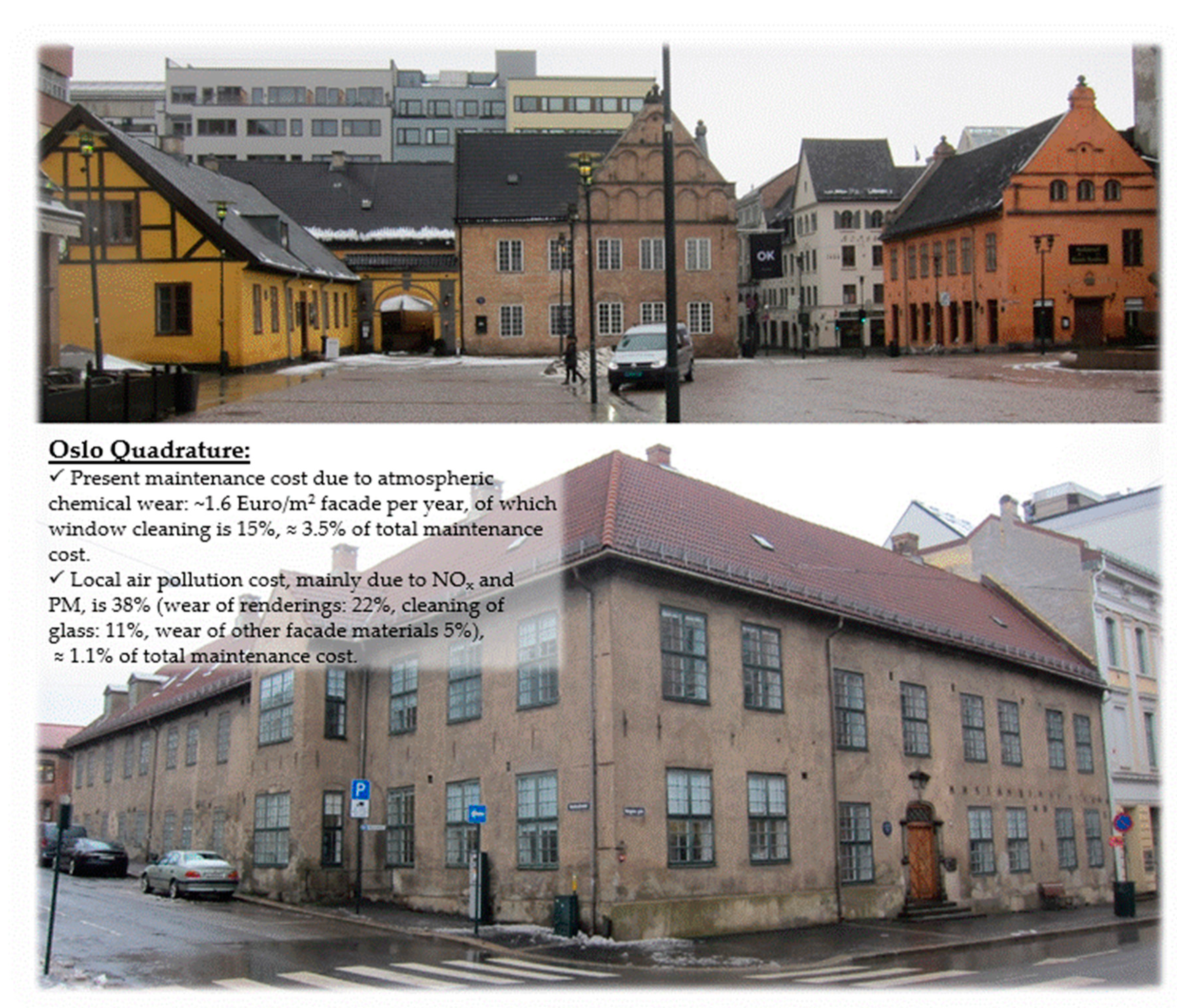
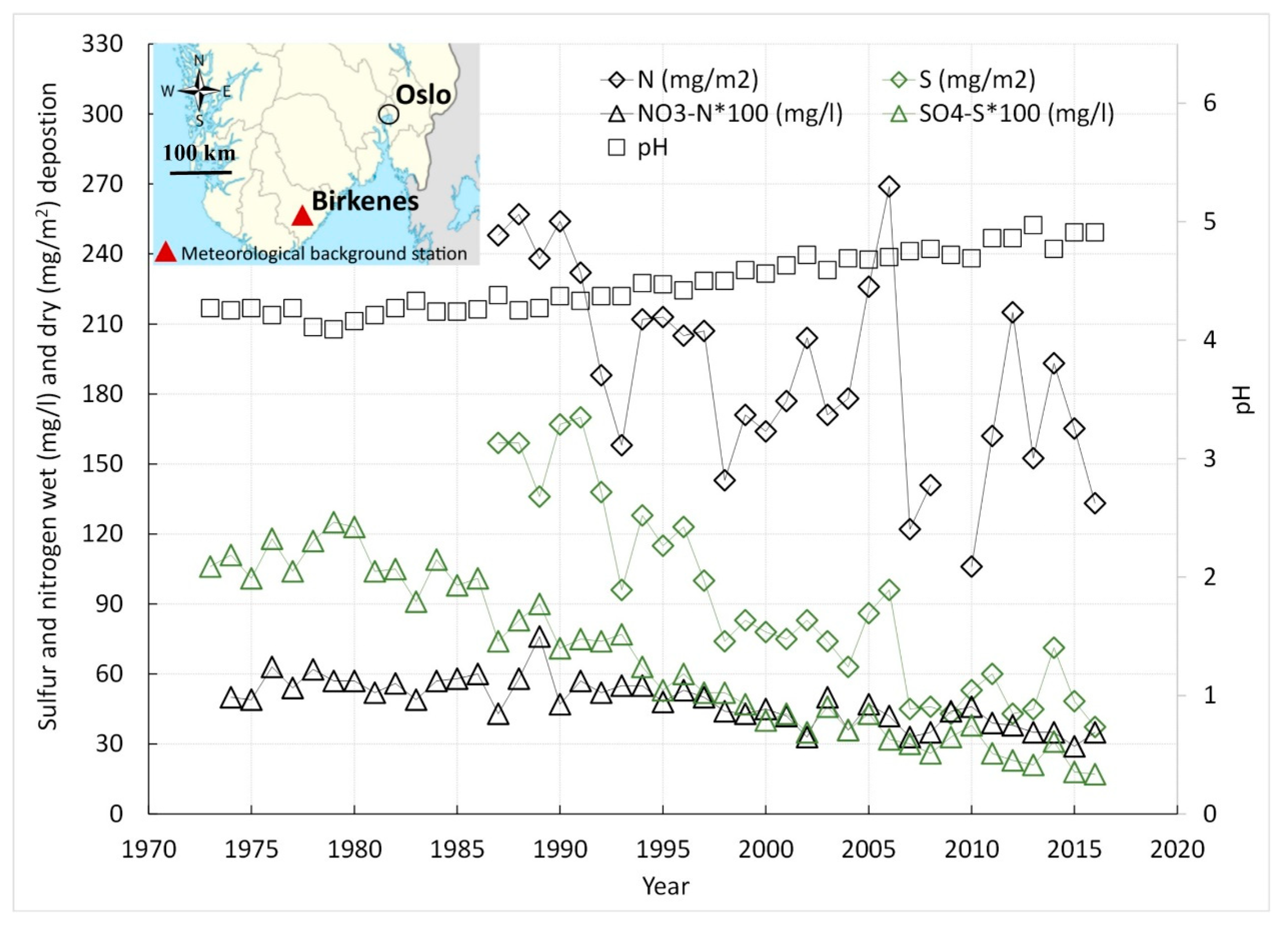
Table 1.
Maintenance cost situations for building façades in the center of Oslo, defined by the ERFs (exposure–response functions) applied for the cost estimations, the type of façade materials and wear process, the estimation years, the maintenance tolerances, and the maintenance costs.
Table 1.
Maintenance cost situations for building façades in the center of Oslo, defined by the ERFs (exposure–response functions) applied for the cost estimations, the type of façade materials and wear process, the estimation years, the maintenance tolerances, and the maintenance costs.
| ERFs | SO2 Dominated Situation | Multi-Pollutant Situation | |||||
|---|---|---|---|---|---|---|---|
| Response material in the ERFs (Footnotes are references to applied ERFs) | The façade materials of 16 buildings in the Oslo Quadrature 1 | Zinc 2 | Portland limestone ornament 2 | Carbon steel 2 | Copper sheet 2 | White painted steel (sheltered) 3 | Modern glass (sheltered) 4 |
| Wear process, W = Weathering, C = Corrosion, S = Soiling | W; C | W: C | W | C | C | S | S |
| Years | 1979; 1995 | 1987–2014 | 2002–2014 | 2002–2014 | 1997–2014 | 2002–2014 | 2002–2014 |
| Maintenance tolerance (R) (µm, % in the case of soiling) | Galvanized sheet: 20-60; Copper roofing: 100; Other materials: Direct lifetime functions without R | Galvanized sheet and monument: 20 1 to 80 5 | 100 5 | 200 6 | 100 1 | 35% loss of reflectance 7 | 3% haze 8 |
| Maintenance costs (Euro/m2, 2019 prices), M = Maintenance, M-C = Maintenance-cleaning, R = replacement | 22–145; Average = 70; Painted rendering (M) = 69; Painted steel and brick (M) = 83; Copper roofing(R) = 124. | 100 9 (M) | 100 9 (M) | 100 9 (M) | 100 9 (R) | 32 10 (M-C) | 2.6 11 (M-C) |
1 [15], all the data in the first column, 2 [20], 3 [21], 4 [22,23], 5 [20], 6 Applied in this work on the assumption that the tolerance for corrosion of carbon steel would be about twice that of zinc. 7 [40], 8 Average first year value over all ICP-materials measurement stations from year 2002 to 2014., 9 An average value for CH surfaces based on [25,41] rounded to 100 Euro was used. 10 [13,14], 11 [25,42].
Table 2.
Values for the air pollutants in the assessed pollution situations in the Oslo Quadrature, defined by the ERFs applied for the cost estimations and the type of façade materials.
Table 2.
Values for the air pollutants in the assessed pollution situations in the Oslo Quadrature, defined by the ERFs applied for the cost estimations and the type of façade materials.
| ERFs | SO2 Dominated Situation | Multi-Pollutant Situation | |||||
|---|---|---|---|---|---|---|---|
| Response material in the ERFs (Footnotes are references to applied ERFs) | The façade materials of 16 Oslo Quadrature buildings 1 | Zinc 2 | Portland limestone ornament 2 | Carbon steel 2 | Copper sheet 2 | White painted steel (sheltered) 3 | Modern glass (sheltered) 4 |
| Pollutants. Annual average concentration (µg/m3), T = Traffic situation, UB = Urban background, RB = Rural background, NR = Not reported, - = Not included in ERFs. | |||||||
| Sulfur dioxide (SO2) | T: 43.4–36.9 RB: 1 | UB: 14.4–0.6 RB: 0.25; | T, UB: 2 RB: 0.25 | T, UB: 2 RB: 0.25 | T, UB: 2 RB: 0.25 | - | T, UB: 2 RB: 0.25 |
| Acidity in precipitation (H+, mg/L), (pH) | T: 0.05 RB: 0.025 | UB: 0.033–0.003 (4.5–5.5) RB: 0.005(5.3) | T, UB: 0.011 (5.0) RB: 0.005 (5.3) | T, UB: 0.011 (5.0) RB: 0.005 (5.3) | T, UB: 0.011 (5.0) RB: 0.005 (5.3) | - | - |
| Chloride, (Cl−, mg/m2·day) | - | - | - | T, UB: 5 RB: 0 | - | - | - |
| Nitrogen dioxide (NO2) | NR (Used to generate O3 values) | - | T: 40 UB: 29 RB: 1.3 | - | - | - | T: 40 UB: 29 RB: 1.3 |
| Ozone (O3) | T: NR RB: 40 | - | T, UB: 35 RB: 60 | - | T, UB: 35 RB: 60 | - | - |
| Particles larger than 10 µm in diameter (PM10) | - | - | T, UB: 21.3 RB: 6 | T, UB: 21.3 RB: 6 | - | T, UB: 21.3 RB: 6 | T, UB: 21.3 RB: 6 |
Table 3.
The materials inventory for the façades of 16 buildings in the Oslo Quadrature, with reported maintenance cost in 1995, according to [15], in 2019 prices (Euro/m2 per year). The values were, in many instances, kept with two digits to show differences, even if this overstated the precision. (i) = materials considered to be inert by [15]. (n.i) = not included in the cost assessment by [15]. * = material for which the cost is shown in Figure 5.
| Material (i = Considered Inert by [15]) | Material Type: M = Metallic, S = Stone/Mineral-Ogical, W = Wooden, O = Other Organic | Area (m2) | Maintenance Cost Due to Atmospheric Wear in 1995 in 2019 Prizes (Euro/m2 per year) | ||
|---|---|---|---|---|---|
| Total Costs | Back-Ground Costs | Local Pollution Cost | |||
| Tile * | S | 895 | 1.4 | 1.4 | 0 |
| Tile, glazed * | S | 2874 | 1.4 | 1.4 | 0 |
| Brick * | S | 15 | 1.4 | 1.4 | 0 |
| Wood, painted | W | 529 | 2.6 | 2.4 | 0.2 |
| Rendering, untreated | S | 108 | 1.88 | 1.81 | 0.1 |
| Rendering, painted * | S | 8213 | 1.94 | 1.9 | 0.04 |
| Stone, mainly granite (i) | S | 1187 | |||
| Glass (i) | S | 2170 | |||
| Aluminium, painted | O, M | 45 | 1.63 | 1.61 | 0.02 |
| Galvanized steel * | M | 78 | 0.8 | 0.5 | 0.3 |
| Galvanized steel, painted | M | 1046 | 1.94 | 1.9 | 0.04 |
| Steel, painted * | O, M | 229 | 11.0 | 10.3 | 0.7 |
| Stainless steel (i) | M | 22 | |||
| Zinc monument (n.i) | M | 50 | |||
| Copper * | M | 1581 | 0.27 | 0.24 | 0.03 |
| Brass (n.i) | M | 16 | |||
| Average, all materials | 19,058 | 1.39 | 1.32 | 0.07 (5%) | |
| Average, degrading materials | 15,603 | 1.69 | 1.61 | 0.08 (5%) | |
Table 4.
Maintenance cost due to atmospheric wear, including multi-pollution exposure, in the period 2002–2014, in 2019 prices. When adjustments were made according to the discussion (see Section 6.1 and Section 6.2) the original value calculated by the ERFs (Figure 5) is given in the brackets. The values for Portland limestone, zinc, and the cleaning of glass are averages for the two situations shown in Figure 5 (Euro/m2 per year). T = Traffic situation, UB = Urban background situation, R0.2 and R0.8 are the cost estimates at recession tolerances of 0.2 and 0.8 mm, as shown in Figure 5.
| Material (i = Considered Inert by [15]) | Material Type: M = Metallic, S = Stone/Mineral-Ogical, W = Wooden, O = Other Organic | Area (m2) | Maintenance Cost Due to Atmospheric Wear (2002–2014) in 2019 Prizes (Euro/m2 per year) | ||
|---|---|---|---|---|---|
| Total Costs | Back-Ground Costs | Local Pollution Cost | |||
| Portland limestone (T + UB/2) | S | - | 1.9 (3.1) | 0.9 (1.5) | 1.0 (1.6) |
| Carbon steel w/ chloride exposure | M | - | 2.0 | 0.3 | 1.7, 1.5 due to Cl |
| Carbon steel without chloride exposure | M | - | 0.25 (0.5) | 0.15 (0.3) | 0.1 (0.2) |
| Zinc (R0.2 + R0.8/2) | M | - | 1.3 | 1.1 | 0.2 |
| Copper | M | 0.3 | 0.2 | 0.1 | |
| Glass, cleaning (T + UB/2) | S | - | 2.0 (4.0) | 0.3 (0.6) | 1.7 (3.4) |
| White painted steel, cleaning | O | - | 1.6 (2.3) | 0.4 (0.6) | 1.2 (1.7) |
| Average, all materials | |||||
| +cleaning of glass | 19,058 | 1.62 | 1.35 | 0.26 (16%) | |
| +Portland limestone as substitute for rendering | 19,058 | 1.62 | 1.0 | 0.62 (38%) | |
| Average, degrading materials | |||||
| +cleaning of glass | 17,773 | 1.73 | 1.45 | 0.28 (16%) | |
| +Portland limestone as substitute for rendering | 17,773 | 1.73 | 1.07 | 0.66 (38%) | |
© 2019 by the author. Licensee MDPI, Basel, Switzerland. This article is an open access article distributed under the terms and conditions of the Creative Commons Attribution (CC BY) license (http://creativecommons.org/licenses/by/4.0/).
Share and Cite
MDPI and ACS Style
Grøntoft, T. Recent Trends in Maintenance Costs for Façades Due to Air Pollution in the Oslo Quadrature, Norway. Atmosphere 2019, 10, 529. https://doi.org/10.3390/atmos10090529
AMA Style
Grøntoft T. Recent Trends in Maintenance Costs for Façades Due to Air Pollution in the Oslo Quadrature, Norway. Atmosphere. 2019; 10(9):529. https://doi.org/10.3390/atmos10090529
Chicago/Turabian StyleGrøntoft, Terje. 2019. "Recent Trends in Maintenance Costs for Façades Due to Air Pollution in the Oslo Quadrature, Norway" Atmosphere 10, no. 9: 529. https://doi.org/10.3390/atmos10090529
Note that from the first issue of 2016, this journal uses article numbers instead of page numbers. See further details here.