Cloud Processing of Aerosol Particles in Marine Stratocumulus Clouds

Abstract

Cloud processing of aerosol particles is an important process and is, for example, thought to be responsible for the so-called “Hoppel-minimum” in the marine aerosol particle distribution or contribute to the cell organization of marine boundary layer clouds. A numerical study of the temporal and spatial scales of the processing of aerosol particles by typical marine stratocumulus clouds is presented. The dynamical framework is inspired by observations during the VOCALS (Variability of the American Monsoon System Ocean-Cloud-Atmosphere-Land Study) Regional Experiment in the Southeast Pacific. The 3-D mesoscale model version of DESCAM (Detailed Scavenging Model) follows cloud microphysics of the stratocumulus deck in a bin-resolved manner and has been extended to keep track of cloud-processed particles in addition to non-processed aerosol particles in the air and inside the cloud drops. The simulation follows the evolution of the processing of aerosol particles by the cloud. It is found that within one hour almost all boundary layer aerosol particles have passed through at least one cloud cycle. However, as the in-cloud residence times of the particles in the considered case are only on the order of minutes, the aerosol particles remain essentially unchanged. Our findings suggest that in order to produce noticeable microphysical and dynamical effects in the marine boundary layer clouds, cloud processing needs to continue for extended periods of time, exceeding largely the time period considered in the present study. A second model study is dedicated to the interaction of ship track particles with marine boundary layer clouds. The model simulates quite satisfactorily the incorporation of the ship plume particles into the cloud. The observed time and spatial scales and a possible Twomey effect were reproduced.

1. Introduction

Aerosol particles are an essential part of the Earth’s atmosphere. They cover sizes from a few nanometers up to tens of micrometers in diameter and are suspended in and transported by air. They are emitted directly as particles at the ground (primary particles) or formed in the atmosphere by gas-to-particle conversion [1]. Aerosol particles are removed from the atmosphere either by gravitational settling (dry deposition) or their incorporation into drops and ice particles and formation of precipitation (wet deposition). Their sizes and chemical composition are largely determined by their formation mechanism [2], comprising salts, organic or biological compounds as well as silicates. Often, their chemical composition is used as a fingerprint to identify the source region of observed aerosol particles [3].

It is commonly accepted that aerosol particles change in size and composition [4,5] due to condensation of gases, coagulation as well as cloud processes [6]. In particular, cloud processing is believed to be an important process in aerosol particle modification. Part of the particulate population can serve as cloud condensation nuclei (CCN) or ice nucleation particles (INP) and are incorporated into the hydrometeors upon their formation [7]. Subsequent uptake of gases and liquid phase chemical reactions, as well as collisions among hydrometers release altered aerosol particles in the air upon cloud hydrometeor evaporation. This evaporation happens at cloud dissipation but also during cloud evolution at the cloud edges and its frequency of occurrence and spatial extension is rather poorly understood and will certainly vary with cloud type and environment.

The long persistence, for example, of marine stratocumulus decks seems to suggest that their drops, and the (particulate or dissolved) pollution mass therein have rather long lifetimes. This assumption, however, is quite incorrect, as even in long-lived clouds renewal and exchange processes can be quite rapid.

Wood [8] in his review summarizes our understanding of marine stratocumulus clouds. He indicates the influence of aerosol particles on cloud droplet distribution, cloud albedo and drizzle formation and states that aerosols in turn are strongly modified by the cloud processes. As [9] suggests, the aerosol particles and the cloud induced changes are the principal driver for the organization of cells in the marine boundary layer. Large-eddy simulations [10,11] have demonstrated that drizzle, initiated by low aerosol concentrations in model simulations, can trigger the formation of open cellular structures. The process is supposed to be accelerated by the steady depletion of the aerosol concentration by coalescence scavenging, that further increases drizzle until a super-clean state is reached [12].

In [13,14] the bi-modal form of marine aerosol particle spectra is studied, and it is attributed to cloud processing. In [13] it is proposed that on the average, aerosol particles participate in 10–20 nonprecipitating cloud cycles over a 3–10 day period, growing to a size of about 0.1 µm before being removed by precipitation scavenging in a rain cloud.

Thus, given the potential importance of cloud processing, the current study aims to shed some light on the temporal and spatial scales of the cycling of aerosol particles in those marine stratocumulus clouds.

In contrast to previous model studies in a similar context (e.g., [11]) our study focuses on the processes at a short time and a small spatial scale, complementing studies, e.g., of [15]. The dynamical framework was largely inspired by observations taken in stratocumuli in the tropical southeast Pacific, such as observed during the VOCALS Regional Experiment [16], in order to provide a realistic context. In particular, we used the thermodynamics and aerosol parameters observed during the C-130 Flight RF06 [17] for a region of open cells with an observed cloud cover of around 60%.

2. Model Description and Initialization

The meso-scale model used for this study is a 3D non-hydrostatic model [18] coupled with the Detailed Scavenging Model DESCAM [7] using a bin-resolved microphysics approach [19]. In contrast to all other bin-resolved studies of a similar dynamical context (e.g., [15]), our model follows explicitly the scavenged aerosol particle mass in the drops and releases them to replenish the ambient aerosol spectrum in case of a complete droplet evaporation.

For the detailed microphysics module, we used the extension of the model that allows to distinguish two different types of aerosol particles [20]. Two aerosol particle size density distribution functions $f_{APa,itype}\left(r\right)$, where $r$ is the moist radius of the aerosol particle of itype = 1 or 2, were considered in the air and their time evolution is calculated from:

$$\frac{\partial f_{APa,ityp}\left(r\right)}{\partial t}={\frac{\partial f_{APa,ityp}\left(r\right)}{\partial t}|}_{dyn}+{\frac{\partial f_{APa,ityp}\left(r\right)}{\partial t}|}_{act/deact}+{\frac{\partial f_{APa,ityp}\left(r\right)}{\partial t}|}_{con/eva}+{\frac{\partial f_{APa,ityp}\left(r\right)}{\partial t}|}_{AP,coll,d}$$

as well as two mass density distribution functions for aerosol particles of itype = 1 and 2 inside the drops $g_{APd,ityp}\left(a\right),$ where a is the drop radius, and their time evolution is calculated from:

$$\frac{\partial g_{APd,ityp}\left(a\right)}{\partial t}={\frac{\partial g_{APd,ityp}\left(a\right)}{\partial t}|}_{dyn}+{\frac{\partial g_{APd,ityp}\left(a\right)}{\partial t}|}_{act/deact}+{\frac{\partial g_{APd,ityp}\left(a\right)}{\partial t}|}_{con/eva}+{\frac{\partial g_{APd,ityp}\left(a\right)}{\partial t}|}_{AP,coll,d}+{\frac{\partial g_{APd,ityp}\left(a\right)}{\partial t}|}_{d,coal}+{\frac{\partial g_{APd,ityp}\left(a\right)}{\partial t}|}_{d,break}$$

As indicated by the subscripts in both equations, the different terms treat dynamical changes: ${()|}_{dyn}$; activation of drops and their deactivation back to aerosol particles: ${()|}_{act/deact}$; evolution involving phase changes due to water vapor diffusion: ${()|}_{con/eva}$, as well as collision process for: ${()|}_{AP,coll,d}$ aerosol/drop collision and ${()|}_{d,coal}$ for drop/drop collision; and finally breakup of drops: ${()|}_{d,break}$. The mathematical treatment of the different microphysical terms can be found in [7].

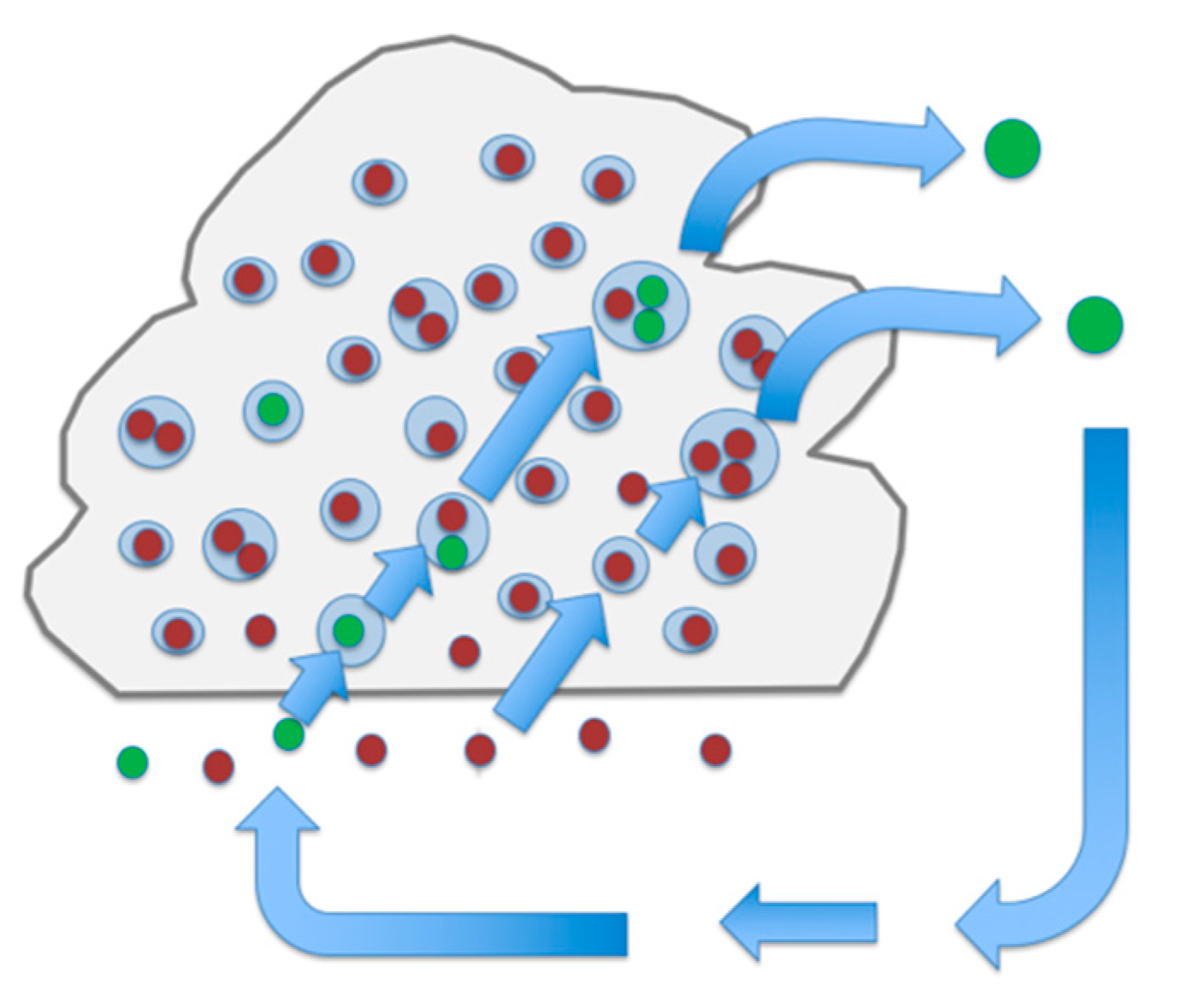
The itype = 1 aerosol particles were the marine boundary layer particles of the initial background conditions (later also called “pristine” particles, indicated in red in Figure 1). They served as CCN for the forming clouds. The itype = 2 aerosol particles were all those that evaporated after having been inside a cloud drop (later also called “processed” particles, indicated in green in Figure 1), regrouping all scavenged aerosol mass into the released particle. They are now treated separately and can later serve also again as CCN, for example. This method allows to follow in detail the fate of the boundary layer aerosol and its cycling through the stratocumulus clouds, in contrast to all previous studies in the literature. As the cloud region is relatively low and warm, no ice phase processes occur.

In a second study, we studied another typical mixing process occurring in marine stratocumulus clouds, associated to ship tracks. We applied the identical setup as before to study the mixing and processing of aerosol particles that were released by an emission line of ship track aerosol (itype = 2), as was observed, for example, during the MAST (Monterey Area Ship Track) experience [21]. The explicit modelling allows to study in detail the mixing of a pollution line into a cloudy marine boundary layer and verify the mixing capacity of the model through comparison with observations, for example, regarding the signature of the plume width.

Due to the rather sophisticated and expensive treatment of the microphysics, the modelling simulation was restricted to only a few hours. Thus, no large-scale changes were considered, even though the model holds a simplified radiation code [22].

In the configuration for simulating a typical shallow marine stratocumulus deck, the model domain covers a volume of 6.4 × 6.4 × 3 km³, with a horizontal grid resolution of Δx = Δy = 50 m and a vertical of Δz = 20 m. The time step Δt is selected to be 1–1.5 s, with a time splitting for the rapid condensation processes. The initial conditions were adapted from [23] (their Figure 1) using a uniform vertical thermodynamic profile with a constant adiabatic temperature of θ = 288 K and a constant water vapour mixing ratio of 7.8 g/kg. Only between 1 km and the inversion at 1500 m potential temperature was slightly increased and humidity decreased, in order to keep the initial atmosphere just below saturation. At the ground a surface latent heat flux of 115 W m⁻² and a surface sensible heat flux = 15 W m⁻² were imposed, within the range of the observed values [17], and random perturbations of 0.1 K and 0.2 g/kg for potential temperature and water vapour mixing ratio were added. No horizontal wind was considered, which corresponds to a model domain drifting along in a large-scale homogeneous environment, moving at a uniform horizontal windspeed.

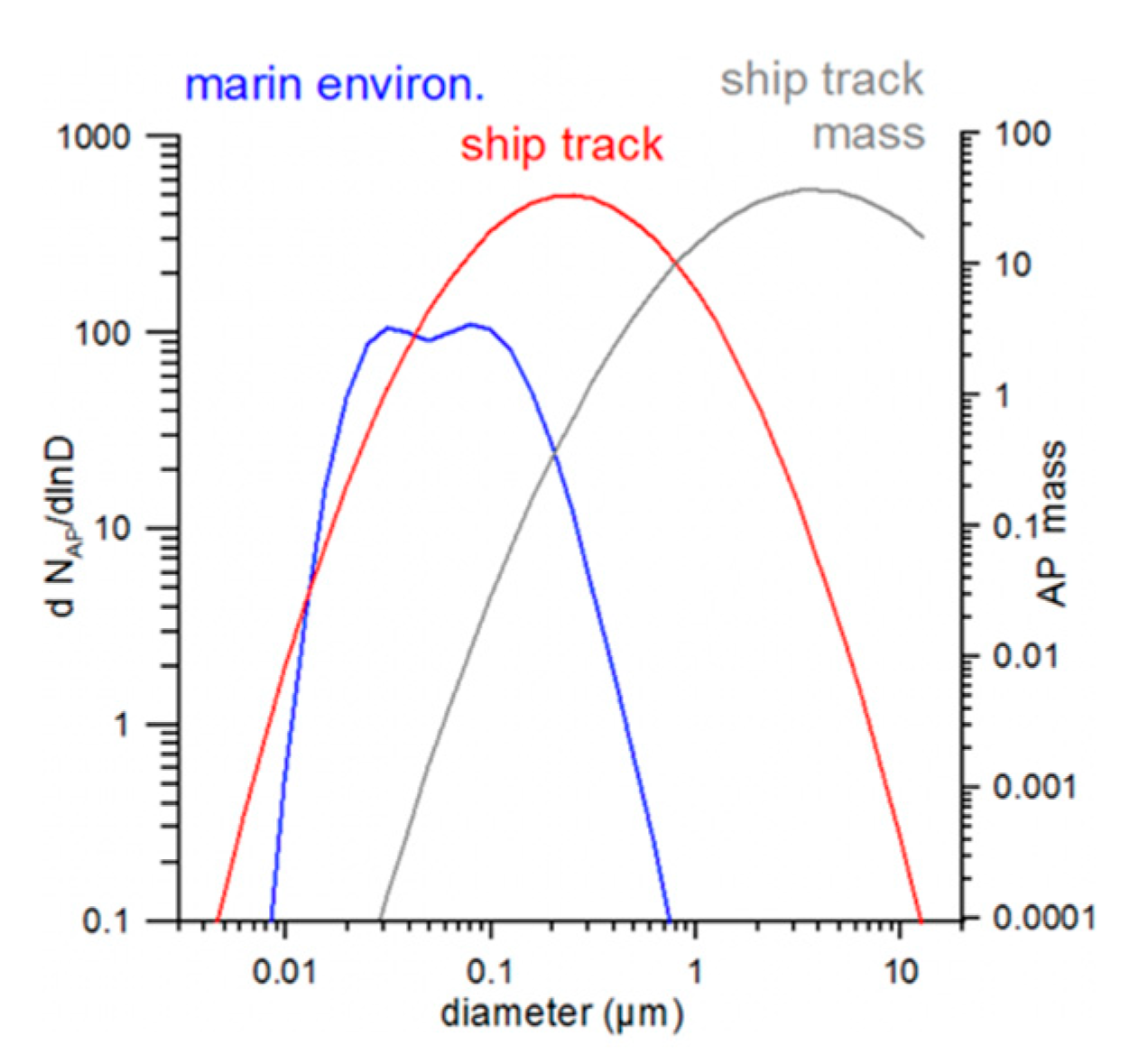
The initial background aerosol particle size distribution (itype = 1) was fitted to the observations of [17] at 1584 m (their Figure 15a) using a superposition of two lognormal distributions for the number of dry aerosol particles N_AP of radius r:

$$\frac{d{N}_{AP}}{d\ln r}={\displaystyle \sum _{i=1}^2\frac{n_i}{\sqrt{2\pi }\log {\sigma }_i\ln 10}}\exp (-\frac{{[\log r/R_i]}^2}{2{(\log {\sigma }_I)}^2})$$

With the values: n₁ = 80 cm⁻³, n₂ = 137 cm⁻³, R₁ = 0.014 µm, and R₂ = 0.04 µm, log σ₁ = 0.146 and log σ₂ = 0.216, the total number concentration is 220 cm⁻³ (Figure 2, blue curve). This particle distribution was observed above the boundary layer, even though observations were equally made inside the boundary layer. We refrained, however, from using those, as they are probably already affected by cloud presence, as will become obvious later. The aerosol particles were initialized constant over the entire domain.

For the ship-track calculations, an additional plume aerosol (itype = 2) with a total of 1200 cm⁻³ (n_p = 1200 cm⁻³, R_p = 0.12 µm, log σ_p = 0.416) was added in the second vertical grid box above ground (between 20 and 40 m) in the center grid line (X = 3 km; Δx = 50 m; Y = 0.8–5.6 km) of the domain (Figure 2, red and gray curve) during 15 s. These aerosol particles are less numerous and slightly bigger than observed by [21], as they are assumed already homogeneous in a grid box of 50 × 50 × 20 m³, and thus somewhat dispersed with respect to the chimney exhausts that were observed.

3. Results and Discussion

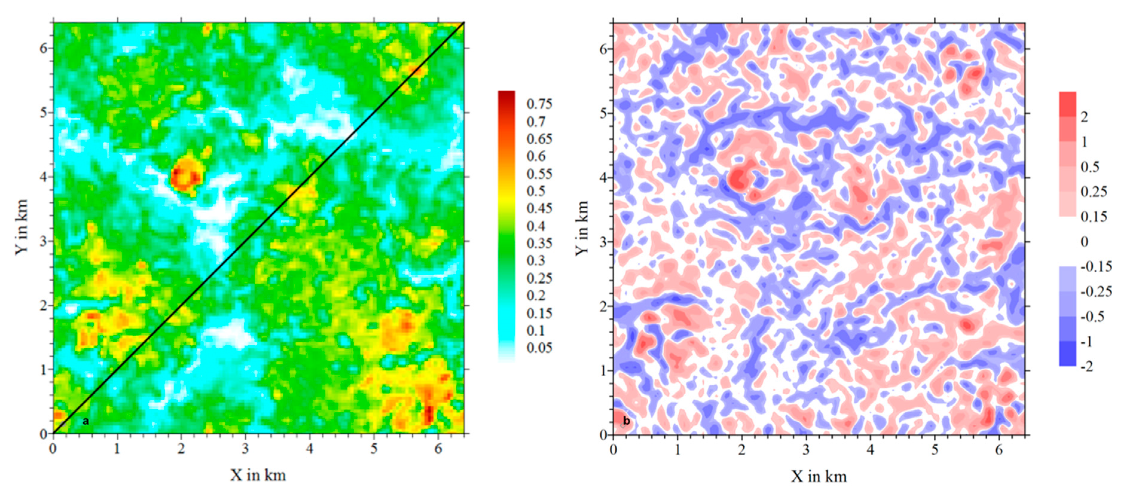
After 120 min of simulation time, a stable situation is reached where cloud cover varies around 65% in agreement with the observations of [17]. A spin-up influence of 2–3 h is also reported by [11]. At 200 min the stratocumulus field just below the inversion is displayed in Figure 3. The liquid water content (Figure 3a) is generally below 0.5 g m⁻³ in agreement with the values reported by [17], with maxima as high as 0.7 g m⁻³ in isolated locations. These regions of high liquid water content correlate to the regions of maximum positive vertical velocity (Figure 3b). Several cells exist, driven by the imposed surface fluxes.

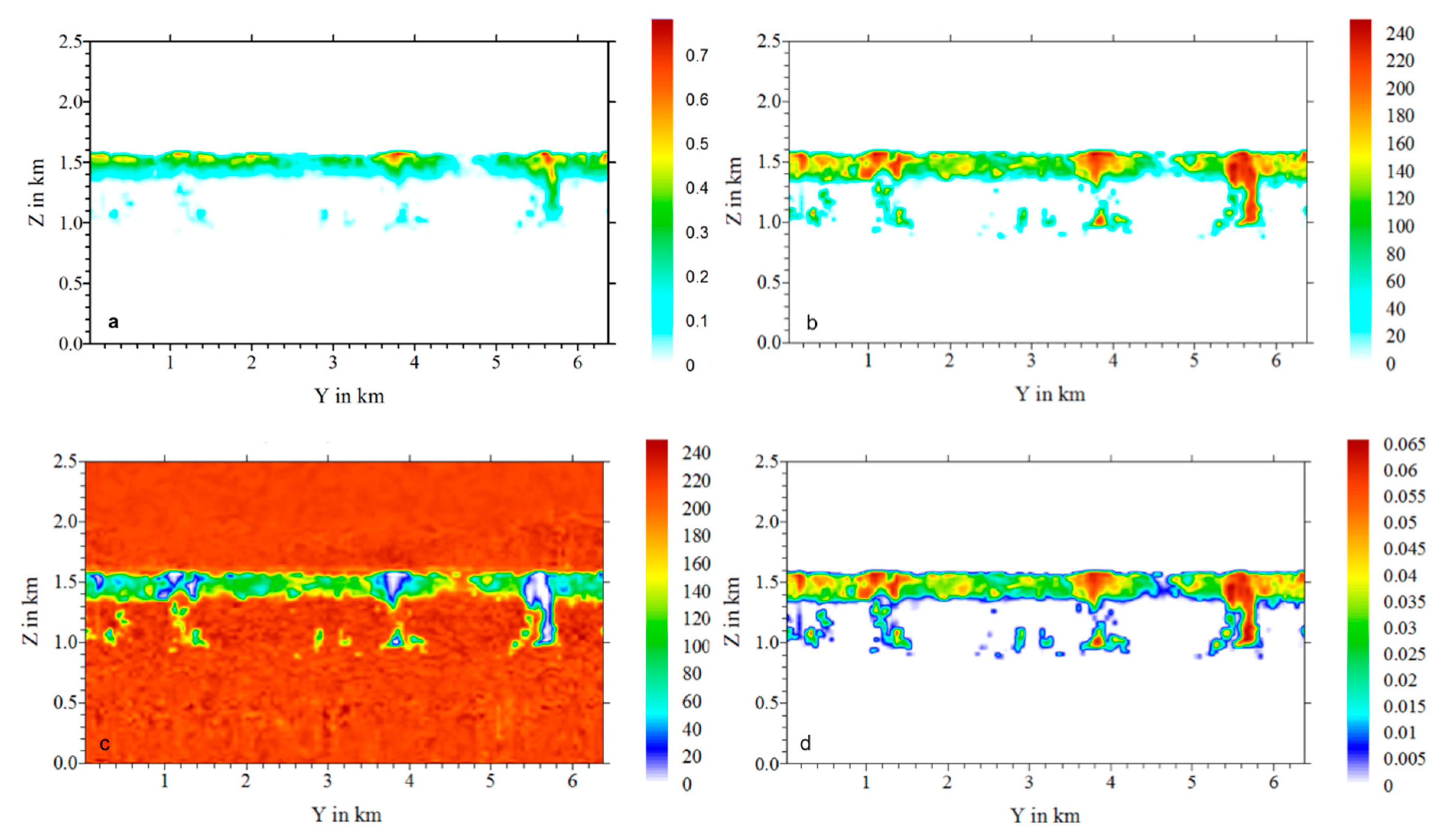
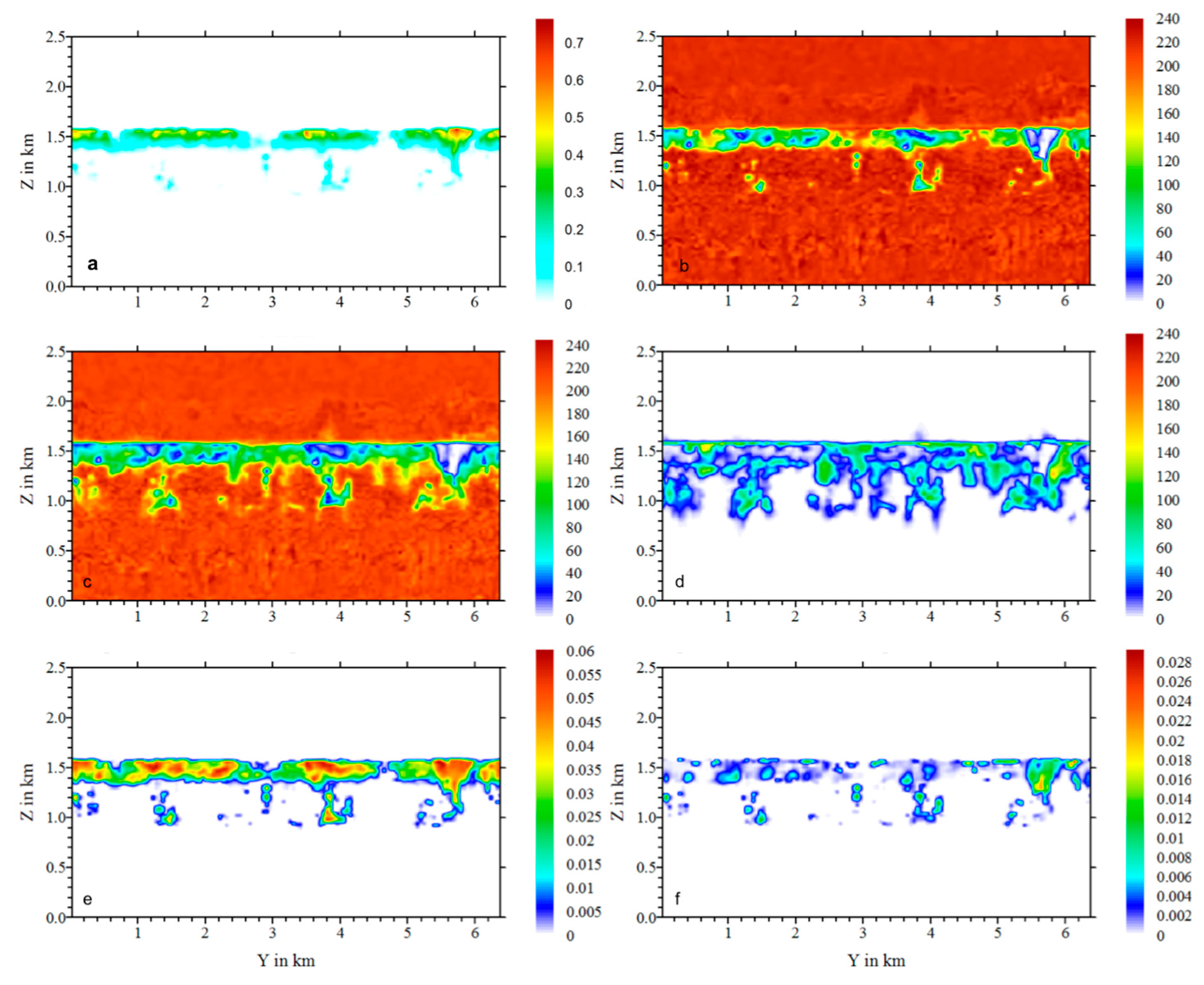
Figure 4 displays some microphysical parameters along the vertical cross section indicated in Figure 3a (black line), but it is projected onto the Y-direction for easier reference. Figure 4a for the liquid water content supports an average value below 0.5 g m⁻³ with a cloud top limited by the height of the inversion. Cloud base can extend down to 1 km while most cloud water can be found in the 300 m just below cloud top, in agreement with [17]. The number of drops (Figure 4b) in the cloud varies with liquid water content and vertical velocity (Figure 3). The highest number concentrations exceeding 200 cm⁻³ are found in the regions of maximum Liquid water content (LWC), while in general drop concentrations are around 100 cm⁻³, exceeding the observed values during this particular VOCALS flight (<50 cm⁻³), while in other similar flights values up to 100 cm⁻³ were also documented.

Figure 4c displays the total number of aerosol particles in the ambient air. The red color represents the initial background particle concentration of 220 cm⁻³ while inside the cloud layer the number concentration has decreased to values below 100 cm⁻³ due to nucleation of droplets. In the regions of high LWC, less than 20 cm⁻³ stay outside the cloud drops in the air, in agreement with the observations of [17]. Figure 4d displays the uptaken aerosol particle mass which can now be found inside the cloud drops.

The cloud at 200 min (Figure 3 and Figure 4) represents the starting point for the following studies. From here on, in the simulation a second aerosol particle type (itype = 2) was opened which accumulates all aerosol particles that are from now on released back into the air after drop evaporation. In the following, these particles are called “processed” particles and they allow to study the evolution of the number and mass of particles that were cycled through a cloud.

The situation after 5 min is given in Figure 5. Figure 5a,b correspond to Figure 4a,c and confirm a globally stable cloud situation. However, Figure 5b for the total number of aerosol particles in the air is now composed of the sum of “pristine” (itype = 1) particles (Figure 5c) and “processed” (itype = 2) particles (Figure 5d) which have already transited in these 5 min of simulation time through one or more cloud stages. The maxima in Figure 5d reach values of 140 cm⁻³, indicating that locally already half of the aerosol number population has been activated into a cloud drop. These particles can be found above 800 m, thus close to the lowest cloud base. Figure 5e and f show the scavenged aerosol mass in the drops of “pristine” (Figure 5e) and already “processed” particles (Figure 5f). The mass contribution of the “processed” particles to the overall uptaken particulate mass on the average is around 10%.

Figure 6a–d shows the same information 35 min later. We note that the ambient aerosol particle concentration of “pristine” and “processed” particles is now affected almost down to the sea surface, even though the geometry of the clouds themselves, as can be perceived from Figure 6c–d, has not changed much and cloud base stays above 900 m. Comparing Figure 6a,b shows that locally almost all particles have already been inside the cloud drops (>200 cm⁻³). In addition, the “processed” aerosol particle mass inside the drops indicates that most of the particle mass has gone through previous cloud events.

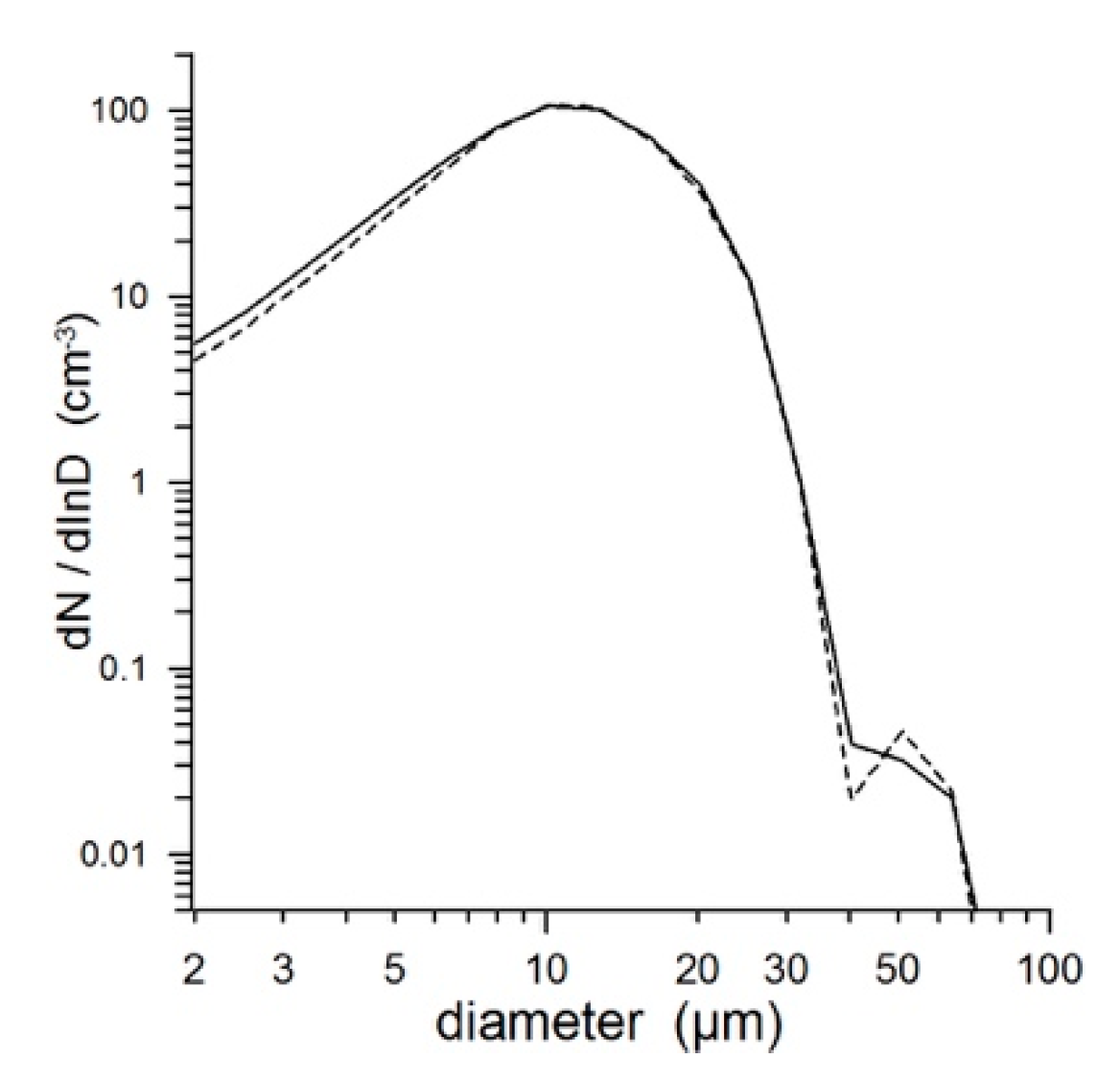
A study of the drop and aerosol particle spectra in the model during the simulation, however, has revealed almost no evolution. Figure 7 shows the mean drop size distribution, averaged over all grid points with a liquid water content exceeding 0.5 mg m⁻³. One curve (dashed line) shows the mean spectrum at the beginning of the processing study (200 min) while the solid one shows the situation 40 min later. The very similar curves show that almost no collision-coalescence broadening of the drop spectum could be observed during this time. Thus, even though Figure 6 demonstrates that a rapid cycling of the aerosol particles through the cloud is happening, the individual particles are in fact affected only very little. Their residence time in the liquid phase is so short (on the order of minutes assuming an average updraft of 1m s⁻¹ (Figure 3b) and a cloud depth of 300m (Figure 4a)) that the drops stay small and almost no collision and coalescence is happening. Thus, the cloud condensation nuclei are released after drop evaporation almost at the same size as they entered the cloud. Very few larger drops have been formed, as the little maximum in the drop size distribution between 40 and 60 µm diameter in Figure 7 shows. However, over the studied time intervals (up to 4 h of simulation), no significant drizzle formation could be observed.

In a second set of simulations, we studied the capacities of the marine boundary layer to mix and process aerosol particles of different origin. Here, the second considered aerosol type (itype = 2) are plume particles as released by ship exhausts [20].

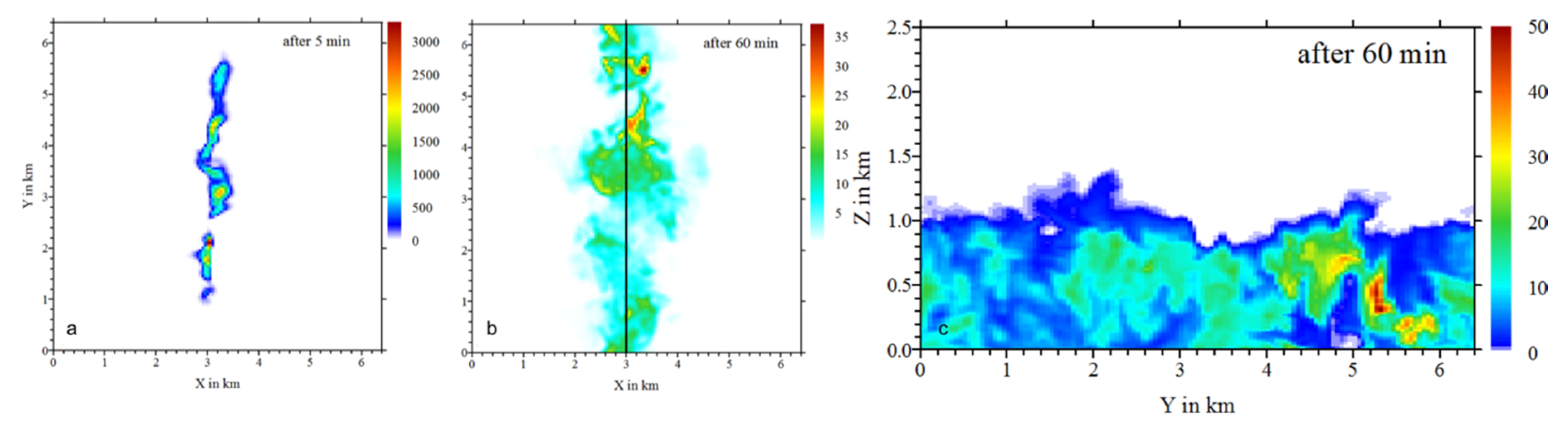
The additional aerosol particles follow a log-normal distribution, as given in Figure 2 by the red curve with a total of 1200 particles cm⁻³. Starting from the same initial state as presented in Figure 3 and Figure 4, these particles are introduced along a line of grid boxes in the middle of the domain during 15 s (see Section 2). Figure 8a gives a horizontal cross section at the height of the release grid box after 5 min. The release line is still very well defined and overall air motion has only somewhat mixed the initial concentrations.

After 1 h of simulation time (Figure 8b,c), the plume has widened horizontally from 50 m to over 2 km, in agreement with observation of [24]. Dilution has decreased the number concentrations to values below 35 cm⁻³. The mixing in an almost neutral boundary layer, however, has transported the particles also vertically. There seems to be a net limit to the transport as the plume number concentrations (Fig.8c) above roughly 1 km are mostly zero. However, as discussed above, the transport continues above 1 km. Here, the large plume particles (see Figure 2 red and gray curve) have been activated into cloud drops.

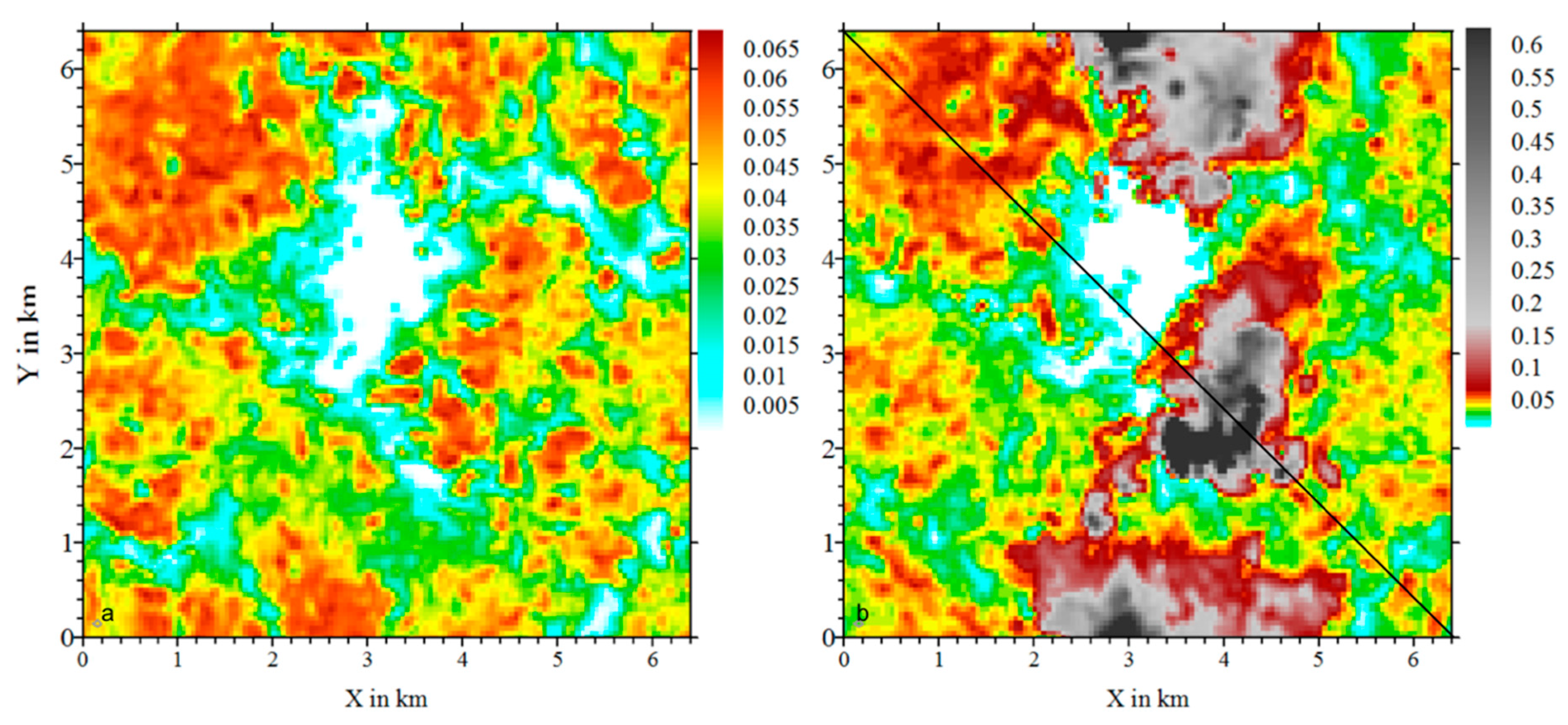
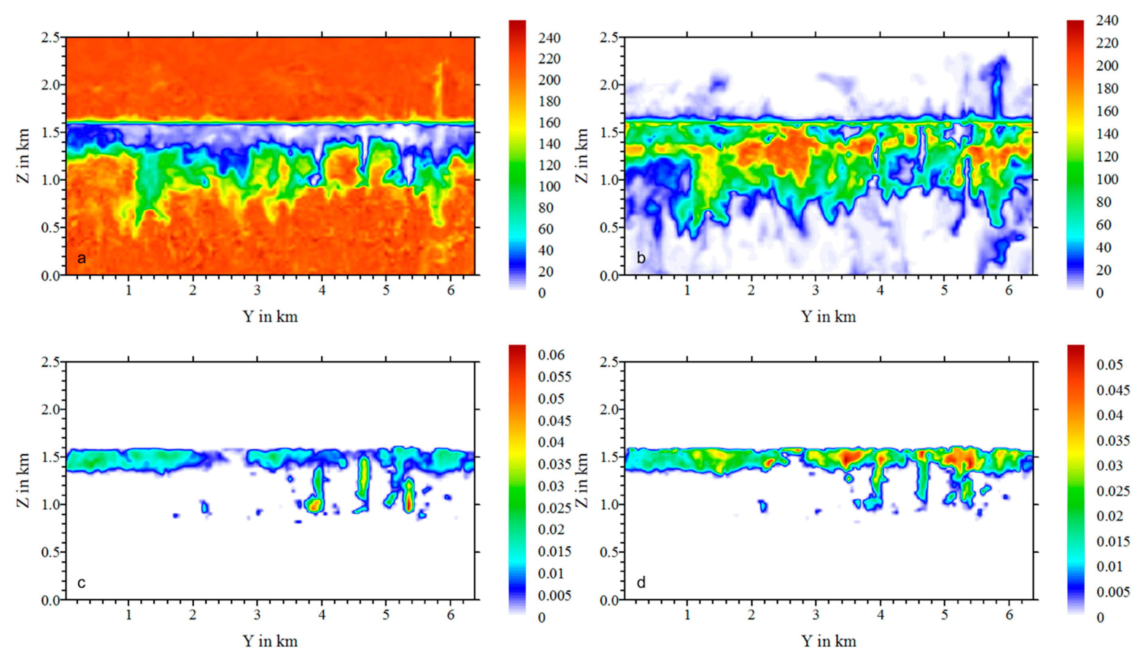
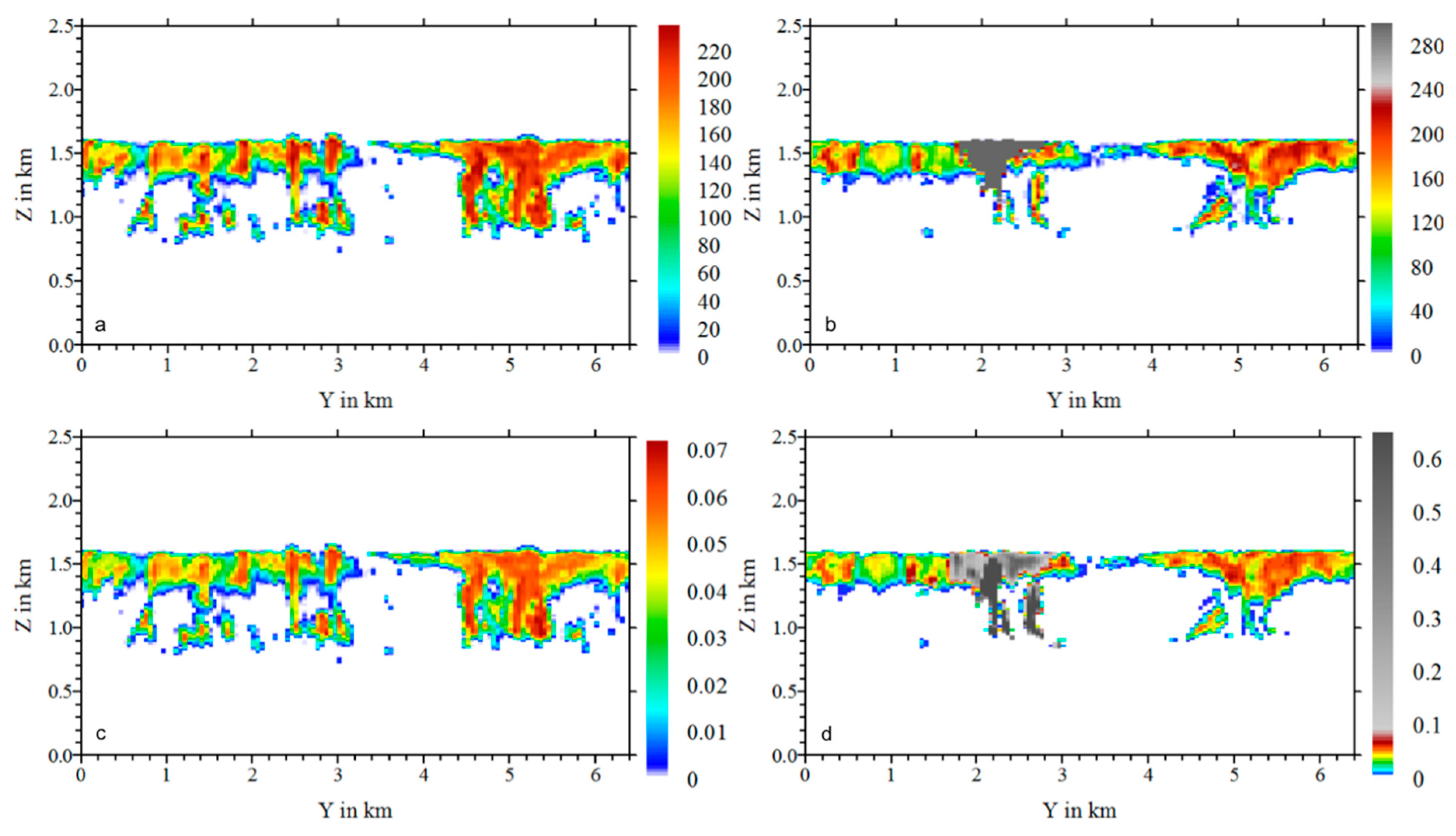
Figure 9a,b present a horizontal cross section of the aerosol particle mass inside the cloud drops at 1520 m. Here, the signature of the plume aerosols is clearly evident. Mass concentrations are 10 times higher than the background concentrations and clearly show the increase of mass due to the plume particles in a region of 3 km width in the X-direction, along the release line. Figure 10 shows the vertical cross section along the black line in Figure 9b where we note an increase of the number concentration of drops by around 50 particles cm⁻³ (Figure 10b) with respect to the background cloud (Figure 10a), in agreement with observations of [20], and an increase in the pollution mass in the drops (Figure 10c,d).

4. Conclusions

A small-scale numerical study of the processing of aerosol particles by marine stratocumulus clouds is presented. The dynamical framework is based on the observations during the VOCALS Regional Experiment [16] in the Southeast Pacific to guarantee realistic meteorological conditions. The 3-D mesoscale model version of DESCAM follows cloud microphysics of the stratocumulus deck in a bin-resolved manner and has been extended to keeping track of two types of aerosol populations in the air and inside the cloud drops.

The aerosol particle spectrum in the boundary layer was initialized with the spectrum observed in the free troposphere with 220 cm⁻³. The formed cloud deck shows an average liquid water content, a vertical extension and a cloud cover within the observed values. The number of drops formed exceeds somewhat the observed values, probably due to the fact that the initial aerosol particle spectrum (observed in the free troposphere) held more particles than observed during this particular VOCALS flight in the boundary layer (100–150 cm⁻³). The model was able to simulate a rapid cycling of the aerosol particles through the cloud affecting almost all particles in the boundary layer within less than an hour. However, with residence times in the liquid phase on the order of a few minutes, the individual particles were much less affected than expected and almost no coalescence effect was observed. During the simulated hour, the aerosol particle spectrum did not broaden, and no “Hoppel”-minimum [13] was yet formed. Furthermore, no formation of drizzle-sized drops was simulated and drop sizes stayed well below 100 µm diameter. Sensitivity studies varying the boundary layer particle spectrum as model input did not change these conclusions.

In the current configuration and with simulation times on the order of only some hours, the stratocumulus cloud, even though very thoroughly cycling the aerosol particle population, did not reduce the number concentration or increase the size of the particles. Considering this small effect of cloud cycling on the aerosol particle population, boundary layer cloud residence times extending towards the longer time estimates of [13] (10 days) seem more realistic to achieve a modification of the aerosol population, while their suggestion of 10 to 20 cloud cycles seems to be largely underestimated. The simulated time scales were not able to change the organization of the boundary layer in cells as has been suggested by [9] for much larger domain sizes and simulation times. Thus, we can conclude that the cycling of aerosol particles through marine stratocumulus clouds for several hours is a lot more rapid than expected, affecting the entire boundary layer, but also a lot less efficient with respect to the broadening of the size distribution of the aerosol particles.

The second study of the mixing of a ship track plume in the presence of the marine stratocumulus deck demonstrated that overall the model performs correctly. The dispersion of the plume in space and time agrees with the available observations [20] and an increase in the number of droplets in the plume track was modelled, suggesting the observed “Twomey effect” [25] as modelled by [26].

Obviously, the cycling times of aerosol particles through clouds depend significantly on the dynamics and thermodynamics of the studied cloud. Here, only a certain type of marine boundary layer clouds was modelled, and the reported behavior is limited to the conditions that were studied. In order to generalize certain findings, different types of clouds in different geographical locations need to be investigated. More findings can be expected when comparing the microphysical response of different clouds with the transition times of individual air parcels through the cloud. In the future, the technique of following different types of particles thorough the cloud phase and the associated mixing will also be used to study other cloud effects due to distinguishable aerosol particle population, such as used for planned and inadvertent pollution events.