Article

An Assessment of the Role of Ice Hydrometeor-Types in WRF Bulk Microphysical Schemes in Simulating Two Heavy Rainfall Events over Southern Nigeria

by
Oluseyi Ezekiel Akinola
1,2 and
Yan Yin
1,*
1
Collaborative Innovation Center on Forecast and Evaluation of Meteorological Disasters/Key Laboratory for Aerosol-Clouds-Precipitation of CMA, Nanjing University of Information Science and Technology, Nanjing 210044, China
2
Department of Physics and Engineering Physics, Obafemi Awolowo University, Ile-Ife 220005, Nigeria
*
Author to whom correspondence should be addressed.
Atmosphere 2019, 10(9), 513; https://doi.org/10.3390/atmos10090513
Submission received: 31 July 2019 / Revised: 23 August 2019 / Accepted: 26 August 2019 / Published: 31 August 2019

Abstract

:
The role of ice hydrometeor-types in bulk schemes available in the Weather Research and Forecasting (WRF) model has been assessed in this study to simulate two heavy rainfall events reported over the southern part of Nigeria. This has been done with a view to provide necessary information on the convective cloud hydrometeor types and compositions in the area to improve heavy rainfall forecasts with the selection of appropriate bulk microphysical schemes. Results from the statistical validation of the simulated rainfall by different schemes showed that for the first event, the WSM5 scheme with less dense snow ice particles performed relatively better than other schemes like WSM6, Morrison with graupel (MORR_G), and Morrison with hail (MORR_H), while the WDM6 scheme performed least effectively when compared to TRMM data. Conversely, the second event showed that a WDM6 scheme with graupel as dense ice particle performed better than other schemes. Further analysis using a spatial distribution plot of simulated rainfall over the area of study shows that for both cases, almost all the schemes fail to capture the intensity and location of the heavy rainfall shown by TRMM data. In addition, the surface accumulated rainfall area average of all schemes for the first (second) event shows an underestimation (overestimation). Vertical profile plots of mass mixing ratios of different ice hydrometeor compositions showed that the WSM5 scheme contains a greater mass of snow than other type ice particles for both cases, while the hydrometeor path calculation of total mass content showed the WSM5 scheme having more snow mass content than other schemes during the period of analysis in both cases. A pressure-time plot of the differences between simulated air temperature and water vapor of the WSM5 scheme showed that WSM5 simulated the higher air temperature that was needed and water vapor at the mid and upper troposphere more than other schemes. In conclusion, results from this study has shown that less dense ice particle (e.g., snow) and high dense ice particle (e.g., graupel and hail) type-bulk schemes can both be suitable for simulating heavy rainfall events that are produced by convective system(s) that are common in the area.

1. Introduction

In the tropical West African (WA) region, rainfall mainly occurs through West African Monsoon (WAM) systems that starts from March in the Gulf of Guinea in the southern part through to around October in the Sahel region. The mechanism that drives the rainfall is mainly convection systems [1], partly due to the day time heating and night time cooling effects that are prominent in the region. Like other parts of the world, occasional heavy rainfall events that often causes excessive flooding are recorded in WA as well [2]. The majority of the past studies on the incidence of heavy rainfall in WA region and Nigeria particularly have mostly considered its social [3,4,5], ecological [6], and climatological [7] impacts. Very few scientific diagnostic studies, particularly those involving the use of a mesoscale model to study the cloud properties composition that produced such a heavy downpour, are available. Research on the cloud types and its composition over this region have been studied during the last two major international field campaign namely; the African Monsoon Multidisciplinary Analyses (AMMA) [8] and Dynamics Aerosol Chemistry Cloud Interactions in West Africa (DACCIWA) [9,10] held in the Sahel and South Western African (SWA) region, respectively. The results from these fields campaign have provided representative information on the identified hotspot of the region which would help to drive global and regional model development in the region.
A mesoscale model on the other hand, can be used to forecast extreme events like heavy rainfall over different parts of the world at short to the long time ranges. Such studies have been conducted over WA too, but most of them did not address cloud hydrometeor compositions of the various bulk schemes in WRF as being partly responsible for why there are differences between the simulated and observed precipitation values. There is therefore a need to undertake such study to provide additional information on cloud types and hydrometeor compositions to weather forecasters over the region, especially the southern part of Nigeria where excessive heavy rainfall is often recorded. The southern part of Nigeria is a coastal area that borders the Gulf of Guinea and Atlantic Ocean (Figure 1). In addition, the area lies in the rain belt region where heavy rainfall is more often recorded than in other parts of the country.
Improvement in weather and climate forecasting with mesoscale models has been achieved, although there is more work to be done, especially with the uncertainty of the complex nature of representing cloud and precipitation processes in those models. The progress made is possible because of the increase in computer power that enables the representation of complex cloud and precipitation microphysics processes within different schemes in the mesoscale model. Most schemes represent cloud and precipitation as either being warm or cold (warm or ice microphysics).
Although the Nigerian Meteorological Agency (NIMET) occasionally forecast heavy rainfall over the southern part of Nigeria, very few of these events have been studied and reported in the literature. This has limited the amount of heavy rainfall cases we can used as a sample to achieve the objective of this study. However, we have considered two previously reported and studied heavy rainfall events as a representative sample. The first heavy rainfall event considered in this study was simulated earlier by reference [11]. The study was aimed at evaluating the performance of the WRF model to forecast heavy rainfall over Nigeria. The study concluded that the rainfall simulated rainfall with the WRF model agreed with some rain gauge stations over Nigeria. Also, the model was able to simulate well the synoptic situations that prevailed during the heavy rainfall. Furthermore, Akinsanola and Aroninuola, (2016) [12] used reanalysis data from the European Centre for Medium-range Weather Forecast (ECMWF) to diagnostically evaluate this particularly heavy rainfall. They found that the heavy rainfall is limited to the south of latitude 9° N and the pre-event days witnessed a strong moisture convergence (divergence) in the lower (middle) troposphere, thereby favoring the upward movement of convectively unstable moist air over almost all the study area. In addition, they suggested that the observation of the African easterly jet (AEJ) at 700 hPa and tropical easterly jet (TEJ) at 200 hPa in the south may have further enhanced the heavy rainfall. Other studies [13] have also identified these two phenomena to be responsible for mesoscale convective systems during the WAM.
The second rainfall event was recorded during the June–July, 2016 DACCIWA extensive field campaign over southern West Africa, which covers part of our study area. This rainfall, according to [14] was caused by “an intense mesoscale convective system in the Guinea Coast region” causing one of the highest ever recorded rainfall amount of about 223.5 mm at a Nigerian southern city of Abakaliki on 12 June 2016. The study only provided a meso-and synoptic scale factors for detailed analysis using a combinations of reanalysis, satellite, and radiosonde datasets. They concluded that over the Nigerian area that is an extremely moist environment, “the mesoscale convective system (MCS) strongly intensified and initiated the formation of a lower-tropospheric vortex thereby causing the MCS to decelerate, resulting in a high rainfall accumulation at the Abakaliki station”. For a full detail description of the rainfall event, see reference [14]. The Level-3 gridded rainfall product of the Global Precipitation Measurement (GPM) called the Integrated Multi-Satellite Retrievals for GPM (IMERG, version 5) with a temporal and grid resolution of 30 min and 0.1° [15] was used for rainfall datasets. However, this study has used the TRMM (TMPA 3B43v7) rainfall product because other studies have justified its suitability over the study area.
We used the WRF model to perform a simulation study of this reported heavy rainfall events with a view to understanding the extent to which compositions of ice microphysics hydrometeor best reproduce the observed rainfall over the region of interest. As noted by reference [16], complex microphysical schemes do not necessarily provide more accurate results than simple schemes. This position was further echoed by [17] who suggested that microphysics schemes that could be suitable for simulating severe thunderstorms in the United States may not be appropriate for simulating warm-type heavy rainfall over the Korean Peninsula. In the context of this assertion, we used four different bulk microphysical schemes (WSM5, WSM6, WDM6 and MORR) with varying degrees of ice hydrometeor compositions to achieve our objective. First, we validated the model simulated rainfall output with TRMM rainfall data using statistical metrics. Furthermore, we evaluated the differences between schemes with mass concentration (and the same ice particle only) and with both mass concentration and number concentration. Finally, we considered the choice between densely rimed-ice particle (hail and graupel) on one hand and low dense ice crystals or snow aggregates on the other hand in simulating the observed heavy rainfall over the study area.

2. Data and Methods

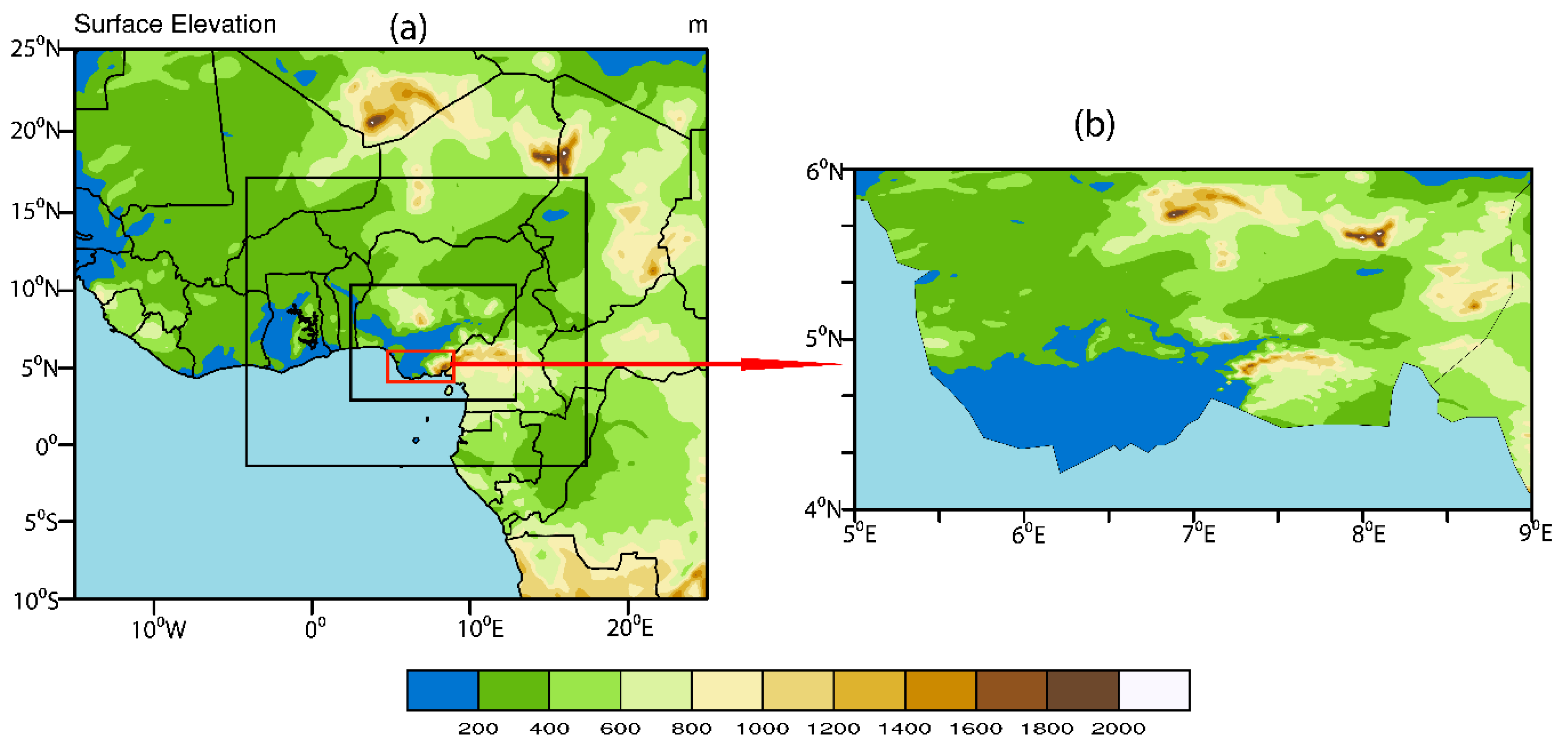
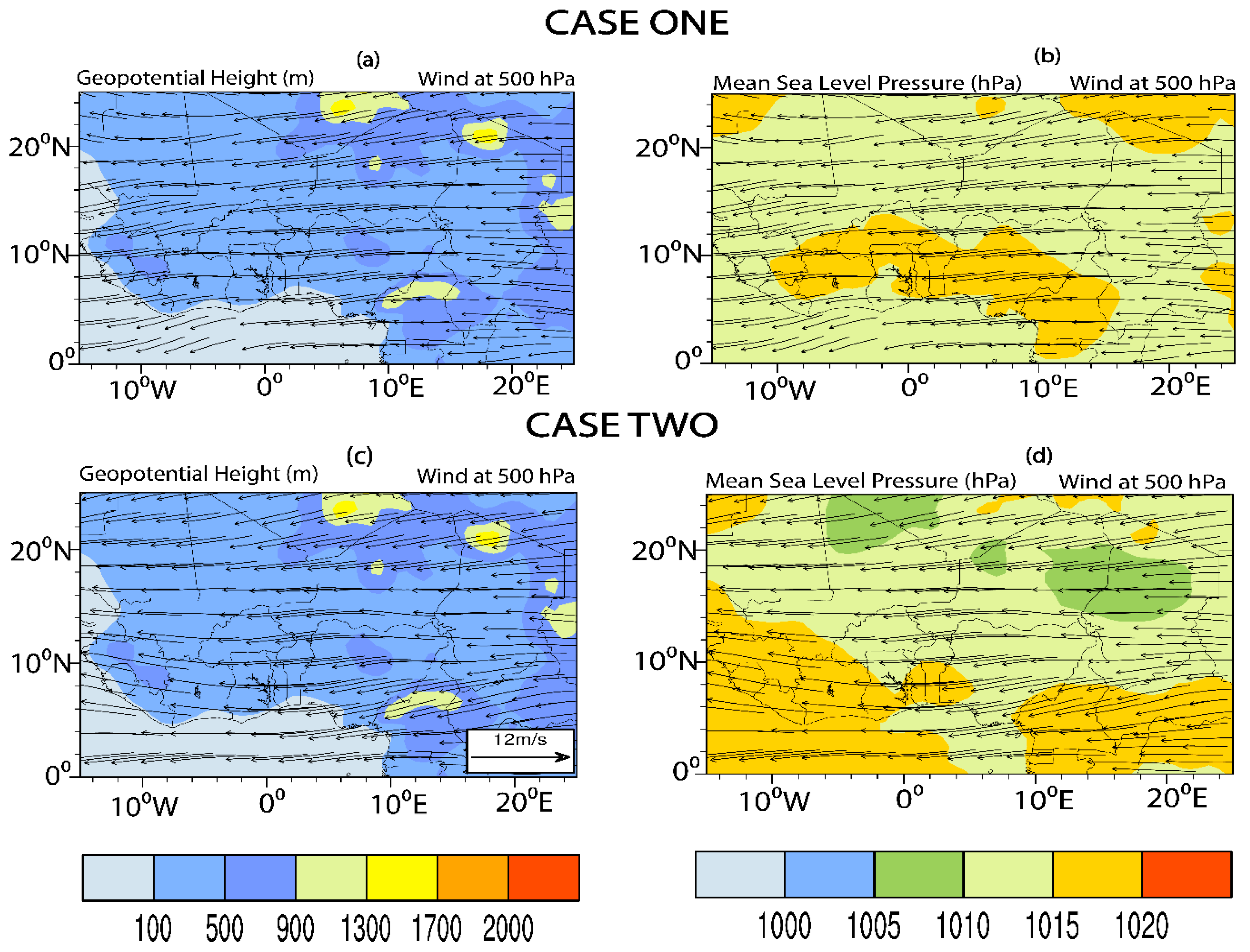
2.1. Heavy Rainfall Events Description and Synoptic Analysis

2.1.1. Case One

During the year 2012 rainy season in WA, there was an exceptionally heavy rainfall event that swept through most of the southern part of Nigeria in West Africa. The Nigerian Meteorological Agency (NIMET) and the National Emergency Agency (NEMA) both reported a huge loss of human lives and material resources to the flooding from the heavy downpour. One of the most affected parts was the southern region of the country. In fact, in 48 h, available meteorological stations recorded an accumulated rainfall amount of about 132 mm/day (Calabar) and 137 mm/day (Umuahia). Reference [12], utilized TRMM (TMPA 3B43v7) and reported that the accumulated rainfall estimates also reached 120mm/day. Considering the previous monthly rainfall record available over this area of 536.3 mm/month (Warri) [18], the downpour can be called heavy. However, due to poor network of rain gauge stations over this part of the world generally, time-tested rainfall satellite data from TRMM would be used for comparison of the simulated rainfall distributions over the domain of study. Figure 2a shows the geopotential height at 850 hPa level (blue solid contour) over the West African domain with a value of about 900 m from ECMWF era-interim data averaged at 06:00 UTC on 28 September 2012. The strong wind (12 m/s) at 500 hPa flowing from the east across our domain of interest is also expected to have contributed to the heavy rainfall later in the afternoon. Figure 2b presents the mean sea level (MSL) pressure with a value of 1020 hPa. The combined impact of these two atmospheric indices is that they created a high-pressure system over the study area and could have enhanced the heavy rainfall that came later in the day around 15:00 UTC on the 28 September, 2012.

2.1.2. Case Two

On 12 June 2016 during the extensive field campaign of DACCIWA in southern West Africa, a Nigerian station at Abakaliki city recorded one of the highest daily heavy rainfall amounts ever recorded at 223.5 mm in 24 h at a near-coastal station. Estimates from the high IMERG rainfall dataset also provide a rainfall amount of around 200 mm, which is very close and consistent with the station record. Furthermore, stations close to Abakaliki recorded substantially lower rainfall amount, making the higher value over the station a localized extreme event. Also, the rainfall was reported to have been produced by long-lived MCS and a moist lower-tropospheric vortex, which originated from the Darfur Mountains in western Sudan and moved rapidly towards the southwest with a high translation speed of 18.3 m/s arriving Nigeria on the evening of 11 June 2016 [14]. A synoptic analysis of the pre-event showing the geopotential height (850 hPa level), mean sea level pressure (850 hPa level) at 06:00 UTC, and the wind speed at 500 hPa on the 11 June 2016 are shown in Figure 2c,d. As in the CASE ONE above, the geopotential height stood at around 900 m (same value as case one), while the mean sea level pressure was at 1015 hPa. The wind at 500 hPa level was strong (12 m/s) and flowed from the east across to west covering the Gulf of Guinea.

2.2. Model Simulations Set-Up

This study used WRF version 3.8 with a ARW dynamical core. The model configuration of one-way interactive triple-nested domains with horizontal resolution and (grid points) of 27 km (174 × 166) for domain 1, 9 km (262 × 217) for domain 2 and 3 km (379 × 217) for domain 3 respectively. In the vertical, 45 levels are used. The conformal map projection is Mercator. The CASE TWO simulations were initiated at 06:00 UTC 28 and the model was integrated for up to 42 h, ending at 00:00 30 September, 2012. The simulation time for domain 1 is 20 s, domain 2 is 6.6 s, and domain 3 is 2.2 s. Both the initial and boundary conditions for ARW model simulations were taken from the National Center for Environmental Prediction (NCEP) Global Forecast System (GFS) datasets available at 1° × 1° resolution and the boundary conditions were updated every 3 h with GFS forecast. The selected period for our analysis is between 15:00 UTC on 28th to 15:00 UTC of 29th September, 2012. Figure 1 gives an overview of the nested model domain used for this study. For CASE TWO, the same model configuration was maintained but with a different initiation time starting at 06:00 UTC 11th June and integrated up to on 42 h ending at 00:00 UTC on 13 June 2016. Also, the period selected for analysis falls between 15:00 UTC on 11th and 15:00 UTC 12 June 2016. To achieve the objective of this study, five experimental simulations (each for CASE ONE and TWO) were carried out with four different bulk microphysics schemes which include WSM5 [19], WSM6 [20], WDM6 [21], and Morrison 2-mom [22]. The WSM5 and WSM6 are both single-moment bulk schemes and they primarily predict the mass mixing ratio of hydrometeors (i.e., cloud water, rain, snow, cloud ice and graupel). The difference between the two schemes is the addition of a high density rime-ice particle graupel to WSM6. The WDM6 scheme predicts both mass mixing ratio (e.g., cloud water, rain, snow, cloud ice and graupel) and number concentration of cloud droplets, cloud ice and cloud condensation nuclei (CCN). WDM6 is classified as partial 2-Moment scheme because it treats only the warm-rain hydrometeors as 2-Moment type while the ice-phase hydrometeor is treated as a 1-Moment type. Its initial value of the cloud condensation nuclei i.e., CCN for the scheme is given as 108 m−3. The Morrison 2-M scheme predicts the mass ratios of (cloud water, rain, snow, cloud ice and graupel) and their respective number concentrations. In addition, the Morrison scheme default high density graupel could be interchanged with hail particle as well as the dense ice type. Table 1 provides the summary of mass mixing ratio and number concentration of variables of all the bulk schemes.
Other physics options used in the simulations include Yonsei University Scheme (YSU) for Planetary Boundary Layer [23] with the Kain-Fritsch Cumulus scheme [24], which was used in the first two domains. In our third domain with 3 km horizontal spatial resolution, simulations were carried out using explicit convection. The Rapid Radiative Transfer Model (RRTM) long wave radiation scheme [25], Dudhia shortwave radiation scheme [26], and Noah scheme for land surface processes [27] were used for longwave, shortwave, and land surface processes, respectively, and they remain unchanged throughout the simulations.

2.3. Dataset Used for Model Validation

The West African region is perhaps one of the most atmospheric data sparse regions of the world due to having inadequate meteorological and synoptic weather stations. Therefore, the usage of station data sets for example, rainfall, is very rare in studies involving model validation over the region. However, the availability of high grade and time-tested satellite rainfall data from the TRMM (Tropical Rainfall Measurement Mission) [28] are often used to replace the inadequate station data. In situ data obtained directly from weather stations still remains the best data for model validation. However, TRMM rainfall data sets have been used for different studies e.g., African Monsoon climatology [29] and many other studies over the region and other parts of Africa and the world. For example, reference [30] used TRMM rainfall data to validate their simulation of an extreme rainfall event over Douala, Cameroon. The TRMM satellite has many rainfall products; here we have used the TRMM 3B42 version 7 stored at 3 h and 0.25° × 0.25° temporal and spatial resolution, respectively. Since the rainfall model output and the TRMM rainfall data do not have the same spatial resolutions, we used the first-order conservative remapping methods [31] to remap the model output to TRMM spatial resolution for easy comparison.

2.4. Methods Used for Model Evaluations

Several statistical evaluation methods are often used to assess model performance. Selection of the most appropriate one to use is often decided by the way the method helps to provide the information needed to answer the relevant questions. In this case, we are interested in evaluating the performance of different schemes with TRMM data to ascertain the ability of these schemes in simulating accumulated surface precipitation over the study area. We selected the following two statistical methods for our validation analysis: the mean bias (MB) and root mean square error (RMSE). These validation statistics have been used in different studies and we will not repeat the derivation of the equations here.
The mean bias (MB) shows the mean for over or underestimation of predictions. The units of measurement are the same as the quantities being considered.
M B = i = 1 n ( O i S i ) n
where S i is the simulated value(s) from the model in our case, O i is the observation value(s) and n is the number of data point used for the calculations.
Root mean square error (RMSE) is also considered for statistical evaluation. RMSE indicates how close the observed data values are to the model’s simulated values. The units of measurement are the same.
R M S E = i = 1 n ( O i S i ) 2 n

3. Results

3.1. Evaluation of WRF Simulated Rainfall

The results of the different statistical metrics used to validate 24 h of surface accumulated precipitation from the 15:00 UTC on 28 September to 15:00 UTC on 29 September 2012 for the two heavy rainfall events from both the simulated and observed data are shown in Table 2. For CASE ONE, it is evident from the results that all the schemes reported an underestimation of the area-averaged accumulated observed rainfall. The least mean bias (MB) value among the schemes was recorded by WSM5 (4.91 mm/day), and WDM6 scheme has the highest mean bias value as −8.56 mm/day while for the other schemes, the MORR_G value is −8.20 mm/day, MORR_H is −8.56 mm/day, and WSM6 scheme value is −7.73 mm/day. The RMSE values of all the schemes is WSM5 (1.74 mm/day), WSM6 (2.83 mm/day), WDM6 (3.03 mm/day) while MORR_G and MORR_H have 3.02 mm/day and 2.90 mm/day, respectively. The mean bias values show that for the accumulated rainfall simulated by the various schemes used in the study, the WSM5 gives the highest area-average accumulated rainfall amount while the WDM6 scheme gives lowest rainfall amount during the period of our study. Other schemes’ accumulated rainfall amount is in between the two schemes. The results of RMSE also confirmed that WSM5 scheme gives the least error among the schemes, which explains its very low RMSE value, while WDM6 gives the highest error. Conversely for CASE TWO, WDM6 scheme recorded the least mean bias of −0.58 mm/day while WSM5 has the highest mean bias of −14.61 mm /day followed by MORR_H (−13.01 mm/day), WSM6 (−6.82 mm/day) and MORR_G scheme with −2.70 mm/day. The results also show the RMSE for the schemes in CASE TWO gives WDM6 value to be 0.20 mm/day making it the least value. This is followed by MORR_G with RMSE value of 0.96 mm/day, WSM6 (2.41 mm/day), MORR_H (4.60 mm/day) and WSM5 (5.16 mm/day).
The above results show that two different schemes perform relatively better for each case used for the evaluation. For CASE ONE, WSM5 has the least mean bias error and least RMSE while for CASE TWO, WDM6 scheme has both the least mean bias and RMSE values. In addition to these two results, one area of convergence is the fact that WSM5 scheme in both cases simulated the highest amount of surface accumulated rainfall, although for the CASE TWO, it overestimated the value from TRMM datasets. The data analyzed only covers the period of our analysis as stated above.

3.2. Role of Ice Hydrometeor on Surface Rainfall Simulations

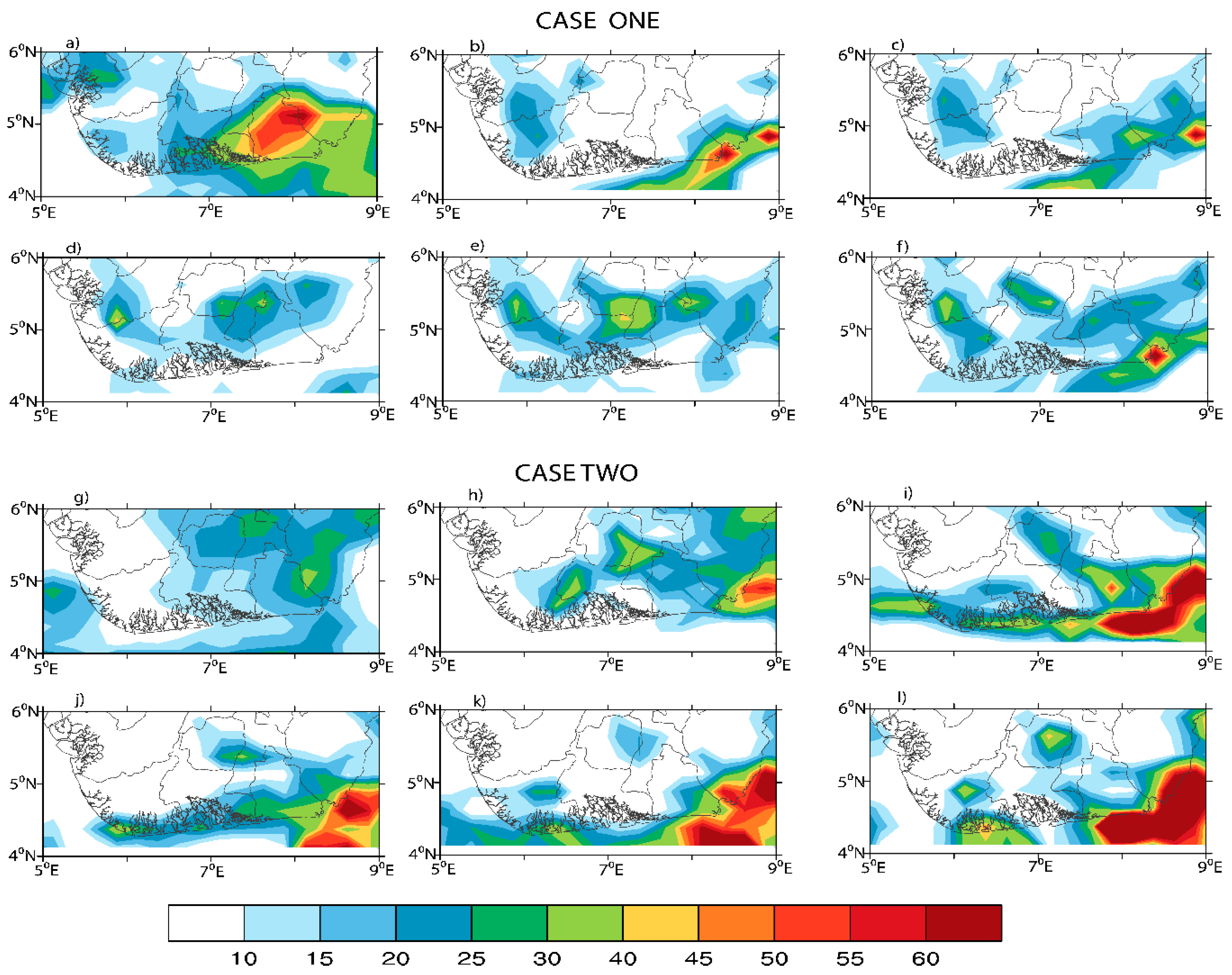
3.2.1. Spatial Distribution of Simulated Heavy Rainfall

The results from using the WRF model to simulate the heavy rainfall events over the southern part of Nigeria with four different cloud microphysical schemes for both cases are shown in Figure 3a–i. Due to insufficient surface rain gauge data over the region and the country in particular, we have used the TRMM 3B42 v.7 as validation data to compare our results from the different schemes. The validation was done after interpolating the rainfall amount datasets from high resolution WRF simulation outputs to the coarse TRMM dataset. Other studies over the region have tested the suitability of the TRMM datasets for comparison with WRF rainfall outputs. For CASE ONE shown in Figure 3a–f, the heavy rainfall recorded and averaged over the (5° N–9° E, 4° N–6° N) area was not captured very well by any of the schemes. The location of the heavy rainfall simulated by MORR_G scheme showed that it fell on the ocean rather than the on continent, as recorded by the TRMM dataset. Other schemes like MORR_H, WSM6, WDM6 and WSM5 showed substantial rainfall distributions, but the intensity is lower when compared with the TRMM. In all, the WSM5 scheme simulated the highest amount of area average heavy rainfall (17.32 mm/day) whereas the amount simulated by MORR_G is 14.03 mm/day, MORR_H (13.68 mm/day), WDM6 (13.67 mm/day) and WSM6 (14.50 mm/day), respectively. The average was for the duration of our analysis only. However, for CASE TWO shown in Figure 3g–i, the performance of the various schemes was different. The TRMM dataset plot given in Figure 3g, showed generally substantial rainfall distributions with lower intensity compared to all the schemes. Like in CASE ONE results, the highest amount of rainfall is simulated by WSM5 scheme while others like WSM6, WDM6, and MORR_H also simulated higher amounts of rainfall but mainly outside of the continental area where the TRMM data showed better rainfall distribution. The only scheme that simulated the continental rainfall distribution as shown by TRMM data is MORR_G, but it still failed to simulate the rainfall distribution over the ocean as shown by TRMM data 3(g). Finally, the total area average of accumulated rainfall simulated by each of the schemes showed that WSM5 is 29.18 mm/day, WSM6 (21.40 mm/day), WDM6 (15.14 mm/day), MORR_H (27.58 mm/day) and MORR_G (17.27 mm/day). The results from these two cases are different from each other with only one area of convergence, which is the simulation of highest accumulated total surface rainfall amount given by WSM5 scheme. The average was for the duration of our analysis only.
For CASE ONE, to show the difference between hail and graupel ice particle, we compared the MORR_G to MORR_H schemes, it was discovered that the distribution of the simulated rainfall by MORR_G is more intense around a particular area while the MORR_H had more distributed lower rainfall values. Replacing the default graupel ice particles in MORR scheme with the hail particle as the rime ice particle changes the rainfall intensity and spread as shown in the Figure 3c. Conversely, the CASE TWO spatial plots given by Figure 3g–l showed that MORR_H scheme 3i simulated more intense heavy rainfall over the ocean which captured the distribution as shown by TRMM dataset, although the intensity of TRMM is lower than the scheme. On the other hand, the MORR_G scheme 3h captured the distribution of rainfall on the continent better than on the ocean when compared to the TRMM dataset.
This process can be explained by considering the fact that graupel density is 400 kg/m3 and hail is 900kg/m3 but the difference is in their velocity–diameter (V–D) relationship which makes hail have shorter suspension time because of its larger fall speed compared to graupel in the atmosphere. For example, the V–D for hail is given as V = 114.5D0.5 while graupel is V = 19.3D0.37. Therefore, for every given same size of hail and graupel available in a cloud, the hail would quickly fall out. According to reference [32], once hail passes through the melting level, a lot of it melts and converts to rain, thereby contributing to the intensity of rainfall over the area. This could be responsible for the spread in rainfall distribution over the study area by MORR_H than MORR_G schemes.
For CASE ONE and TWO, the rainfall simulated by WSM6 scheme showed more spread and a more intense rainfall distribution than the WDM6 scheme although both of them show the same ice species mixing ratios (ice, cloud and graupel) with the additional number provided by the WDM6 scheme. The result is different to other studies over different parts of the world. For example, reference [33] simulated heavy warm-type rainfall over Korea Peninsula, they concluded that WDM6 scheme simulated rainfall more effectively than the WSM6 scheme. Reference [32] also simulated a mesoscale convective system over US Great Plain with the two schemes and they concluded that WDM6 scheme performs better, especially with rainfall from medium–to–heavy rainfall. According to reference [34], the enhancement to the warm rain physics in the WSM6 scheme made it suitable for strengthening heavy rain activity. In addition to this, the WDM6 scheme also provides cloud condensation nuclei (CCN). We speculated that it may have played a crucial role in the underestimation of the simulated rainfall. The area of our study is known for its oil exploration and gas flaring [35,36] which makes it one of the most polluted parts of Africa due to an abundance of aerosols concentration. According to reference [37], when cloud droplets and aerosols interact, they form numerous but smaller, droplets for a given liquid water content resulting in larger cloud albedo called the first indirect effect. Reference [38] further opined that the resulted decrease in cloud droplet sizes could result in the precipitation processes being delayed and reduced, which is now referred to as the second indirect effect. Since the focus of this study is not on aerosol-cloud interactions, that area is left for another study. The performance of WDM6 and WSM6 schemes over this region is further examined with the analysis of vertical profiles and hydrometeor paths later for both cases.
Furthermore, to test how graupel particles in (WSM6 and WDM6) contributed to the simulation of the observed heavy rainfall events, an earlier version WSM5 scheme was used. The WSM5 scheme is mixed-phase type scheme updated to WSM6 scheme with the addition of graupel as additional predictable variable to make it a more complex scheme. WSM5 scheme has snow as its dense ice particle. From our results given is Figure 3e,f,k,l, WSM5 scheme simulation of the heavy rainfall is intense and spread out when compared to the WSM6 scheme and even WDM6 for both cases, even though for CASE TWO, they both fail to capture the simulation on the continent as shown by the TRMM dataset. As stated earlier, graupel V–D makes it have a longer residency time than other ice hydrometeors. For CASE ONE however, the general performance of all the bulk microphysics used totally underestimated the observed rainfall while results from CASE TWO showed that all the schemes used (MORR_H, MORR_G, WDM6, WSM6 and WSM5) overestimated the rainfall estimates from TRMM rainfall dataset over the selected location used in this study. The inconsistencies in the results from the two cases showed that simulating physical phenomenon like heavy rainfall which can be produced by different physical mechanisms like MCSs, tropical cyclone and hurricanes among others using mesoscale WRF models with cloud and precipitation microphysical schemes is still a challenging task. It further shows that the proper representation of cloud and precipitation properties and processes in cloud models is very crucial in modeling studies, as well as proper diagnostic study of the microphysical compositions of such a phenomenon and the producing mechanisms. Future studies should use rain gauge as well as and radar datasets, which are presently not available over the region for validation purposes. Therefore, the spatial distribution of the simulated aggregated rainfall as shown above (Figure 3) has limited applications.

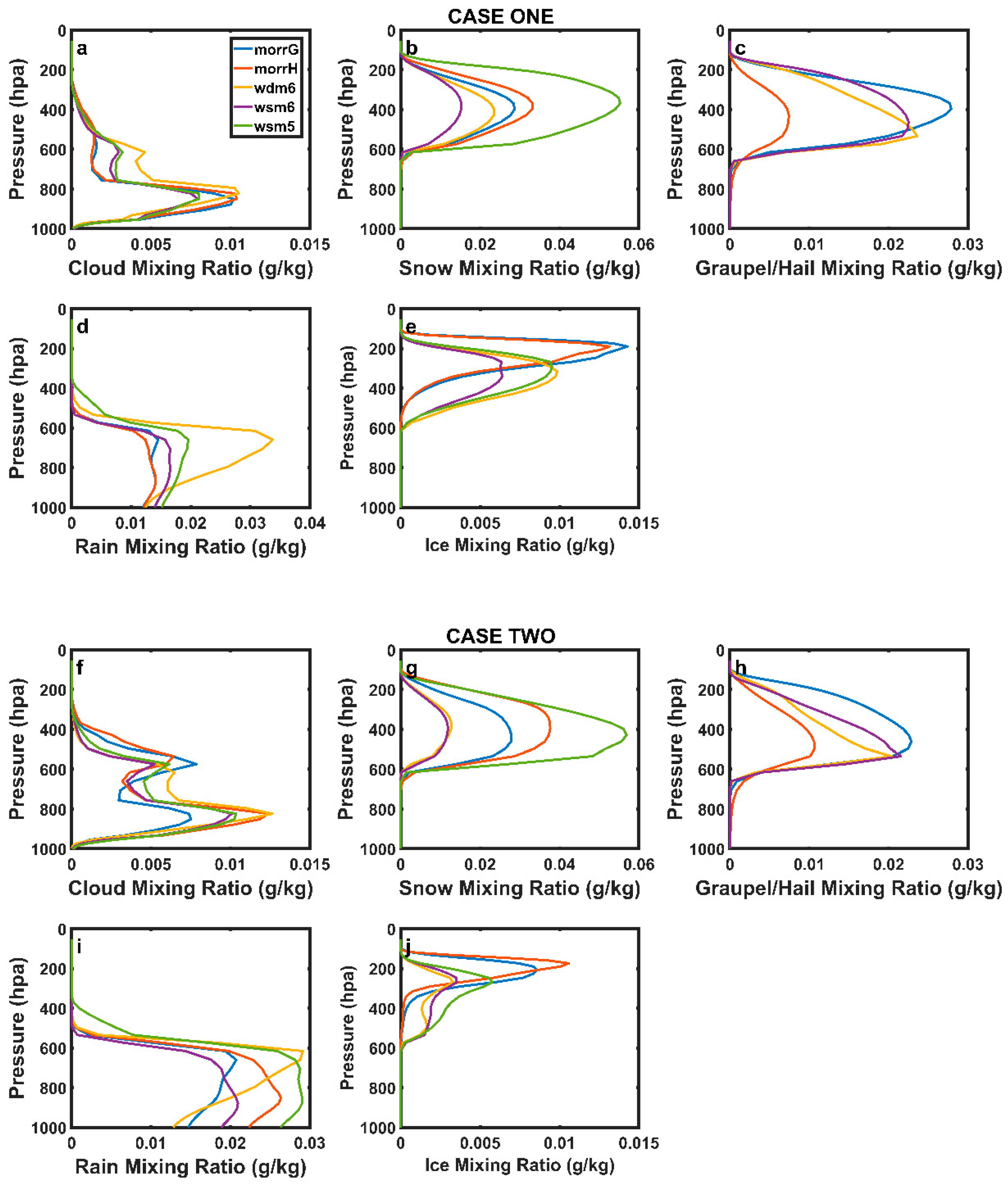
3.2.2. Area Average Vertical Hydrometer Compositions

The performance of different bulk schemes with varying ice hydrometeor categories in simulating two cases of heavy rainfall over southern Nigeria as shown by the spatial distributions of the resulting precipitation needs to be further analyzed. Here, we presented the area averaged from different hydrometeor mixing ratios prognosis by each of the bulk schemes used. The data used was averaged over the study area (5° N–9° E, 4° N–6° N) for 24 h period for the two cases. The vertical profile plots, Figure 4a–j provide insights into the vertical variabilities in the magnitude of the various hydrometeors prognosis based on each scheme. For CASE ONE, Figure 4a shows the cloud mixing ratio of all the schemes used and how they varied vertically. The high concentration of the cloud mass in the lower troposphere may have impacted the rainfall produced by all the schemes. For example, MORR_G, MORR_H and WDM6 schemes simulated more cloud mass in the lower troposphere (about 0.01g/kg) compared to WSM6 and WSM5 schemes (0.0075 g/kg). This is contrasted to how MORR_G and MORR_H schemes simulated cloud mass at mid-troposphere which is far lesser (0.0025 g/kg). Unlike the CASE ONE above, virtually all the schemes simulated more cloud mass in the mid troposphere for the CASE TWO shown as Figure 4f, although the values vary with MORR_H and WSM6 schemes cloud mass value of about (0.005 g/kg), while MORR_G has about 0.008 g/kg. The simulated cloud mass by MORR_H and WDM6 at the lower troposphere for CASE TWO is larger than CASE ONE reaching a value of about 0.013 g/kg. Persistence cloud cover could be resulted from delay in precipitation processes from initiation. In addition, collision-coalescence is the main warm-rain formation mechanism [39] which operates in clouds containing droplets irrespective of whether they are above or below 0 °C.
Figure 4b,g shows the snow mixing ratio from all the schemes in both cases ONE and TWO, it could be seen that WSM5 produced more snow while WSM6 scheme produced the least snow and the other three schemes are intermediate. As was stated before, the density of snow and its V–D relationship could have been responsible for this outcome.
Figure 4e,j shows the ice mixing ratio profile of the bulk schemes for both cases used in the study. Both MORR_G and MORR_H schemes exhibit a much larger amount of cloud ice in the upper troposphere but much smaller amounts of snow slightly above the mid-troposphere. As stated by reference [40], the basic dynamic mechanism of hydrometeors advection in a typical mesoscale convective system (MCS) is the relative flow from the convective core to the outer region in the upper level. Reference [32] demonstrated this in the simulation of MCS over Southern Great Plain in the USA, by using a MORR scheme. Our results have further confirmed the ability of MORR (H and G) in simulating upper-level ice-phase hydrometeors because of its larger upper-level horizontal wind speed than other schemes. According to reference [32], the high horizontal wind speed and small hydrometeor fall speed could be responsible for the ice-phase particle to spread out into larger region. The ice-phase hydrometeors of WDM6 and WSM6 are however different from MORR (G and H) in both cases. However, the amount of ice masses simulated by the two schemes in CASE ONE, Figure 4e are much larger than that simulated by the schemes for CASE TWO. In fact, compared to ice mixing ratio profile from the WSM6 scheme, the WDM6 scheme exhibited a larger amount of ice cloud mass than the WSM6 scheme. Also, WSM6 exhibited less snow compared to WDM6. However, in CASE TWO, both WSM6 and WDM6 schemes exhibited almost equal amount of ice mass as shown in Figure 4j.
The fact is that both WSM6 and WDM6 utilized temperature-dependent intercept parameters for the snow and mass-dependent cloud ice number concentration, unlike the other schemes [17]. The snow mass mixing ratio of WSM5 scheme exhibited a larger amount compared to other schemes. As said before that snow in WSM5 schemes could melt and directly produce rain water. This could thus be responsible for the scheme ability to simulate more accumulated precipitation than other schemes. The graupel mixing ratio is shown in Figure 4d,h for all the schemes in both cases. MORR_G scheme exhibited a larger graupel amount than the duo of WDM6 and WSM6, which also prognosis graupel as a dense rime ice particle for simulating cloud and precipitation. The hail mixing ratio from MORR_H scheme exhibited a lower mass amount compared to the MORR_G scheme. For the rain mixing ratios, while in CASE ONE all the schemes exhibited rather intermediate rain mixing ratio values in the mid-troposphere except for WDM6 schemes with a much larger ratio value, the CASE TWO rain ratios from all schemes show a much larger values Figure 4i. In conclusion, the WSM5 scheme in both cases produced the largest rain mixing ratio values at the surface. This further confirmed that the WSM5 scheme simulated relatively more surface accumulated rainfall amount over the study area.

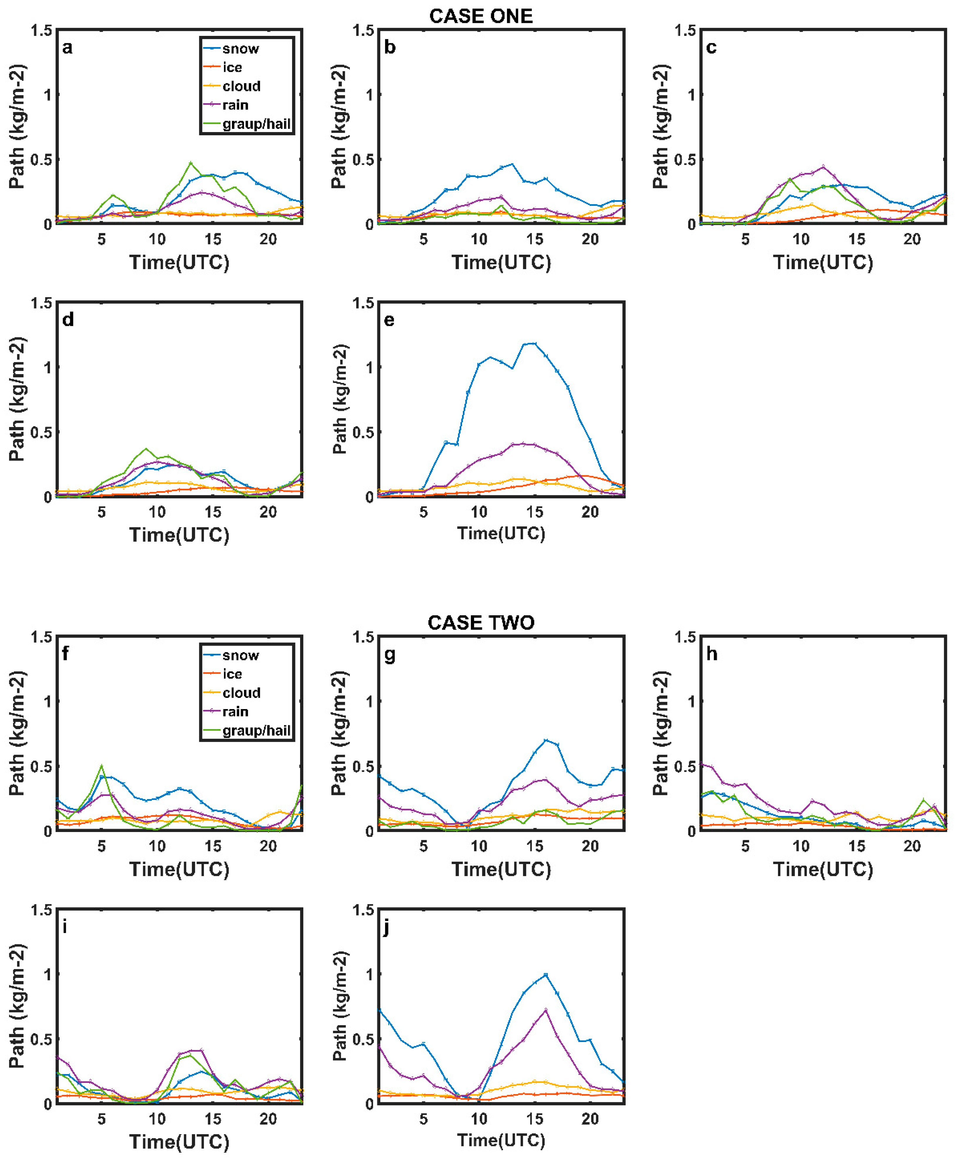
3.2.3. Hydrometeor Path Calculations

The change in results produced by different ice hydrometeors (hail, graupel, snow, and ice) in bulk schemes used in the simulation of heavy rainfall events over our study area need further examination. The hydrometeor numbers and distributions are analyzed using the hydrometeor path (HP) calculation. HP is used to represent the total mass content of the sum of the hydrometeors over the whole depth of an atmospheric column [41] and is given as:
H P = 0 z p i q   d z
where q represents the hydrometeor types (e.g., cloud, ice, rain, snow, graupel, hail), p i is the air density at sea level given as 1.22 kg/m3 and z is the model level of integration.
The time series of the calculated area averaged hydrometeor path of all the schemes for both cases are shown in Figure 5a–j. The analysis is done in two parts: graupel–hail and snow–graupel. For graupel–hail, the calculated HP of MORR_G and MORR_H are examined to provide further insight as to why simulations done with graupel as a dense rime ice particle simulated heavy rainfall amounts that were more than that of hail as a dense rime ice. For CASE ONE, Figure 5a shows that the calculated path of graupel in MORR_G is larger with a maximum value of about 0.5 kg/m2 compared to hail in MORR_H Figure 5b with a path maximum value of about 0.1 kg/m2. Furthermore, the path of the total rainfall is also impacted by the amount of snow in the atmosphere at a particular period since it can be collected by aggregation as it falls through by both hail and graupel. Snow density is 100 kg/m3 with a V–D value of 11.72D0.41, thereby making snow have a lower fall speed compared to hail and graupel. The contribution of snow to heavy rainfall by MORR_G scheme may not have been possible because both graupel and snow almost have the same HP maximum value of 0.5 kg/m3 making it possible for graupel to collect some snow particles by the process of aggregation as it falls. After the path of snow and graupel peaked, they both dropped in value but the snow still maintained a higher value into the later time. The drop seen in the HP of graupel may be responsible for the quick simulation of the rainfall as all the graupel particles could have fallen out before they get to the continental area, as shown by the TRMM plot in Figure 3a. This is evident from Figure 5a above because there is a reduction in rain mass mixing ratio with graupel mass particle drop in MORR_G scheme. On the other hand, hail in MORR_H scheme has a lower HP value of about 0.1 kg/m3 compared to graupel (0.5 kg/m3). Hail, as a high dense rimed ice particle, falls out quickly than snow with a peak PH value of almost about 0.5 kg/m3. This we speculated could be responsible for the slightly lower rainfall recorded for MORR_H scheme with the addition of snow HP value since hail could also collect snow by the aggregate process while falling. Consistently with results from spatial distribution of rainfall as shown in Figure 3c, MORR_H scheme shows better spatial distributions compared to MORR_G scheme in simulating the heavy rainfall studied with a slightly lower total accumulated rainfall area average. Also for CASE TWO, the time series plot of calculated HP for graupel–hail part followed a similar pattern as CASE ONE as shown in Figure 5f,g although with some variations in the magnitude of the simulated HP values. For example, the HP of graupel from MORR_G scheme has a maximum value of about 0.5 kg/m3 within the first 5 h into the simulation, the calculated HP for hail from the MORR_H maintained a lower value of around 0.1 kg/m3, however, the HP for rain showed a higher value, thus making the MORR_H produce more surface accumulated rainfall than MORR_G scheme. This is contrary to CASE ONE where the latter produced more surface rainfall. In addition, as noted in the CASE ONE above and also observed in the CASE TWO, the total amount of rainfall is impacted by the total amount of snow mass available in the atmosphere at a particular time.
Furthermore, the HP for snow–graupel of CASE ONE in Figure 5d shows that the calculated WSM6 scheme HP for snow was lower than HP of graupel until around 10 h into the considered time of our analysis (11:00 pm local time of 28 September) before the graupel HP dropped, making the rain mass mixing ratio also drop. As explained in the graupel–hail comparison above, the V–D relationship of graupel and its density make it fall out quickly when compared to snow, thereby possibly reducing the mean precipitation as time goes by as seen in Figure 5d above. Another reason why the precipitation simulated by WSM6 scheme is lower than WSM5 scheme is due to the process of conversion from cloud particles to graupel and the melting process needed to produce precipitation that could be longer because in WSM5, cloud particles can convert directly and quickly to precipitation [19]. In addition, the calculated HP of snow hydrometer in WSM5 scheme has a unique value of about 1.2 kg/m3 at 11:00 UTC before falling drastically down. For CASE TWO, time series plot of the calculated HP for snow–graupel part of the analysis is shown in Figure 5h,i. A similar pattern as shown in CASE ONE is also observed in CASE TWO, either the calculated HP of snow in WSM5 scheme reached a high value of about 1.0 kg/m3 at 17:00 UTC before dropping down.
The WSM5 scheme is a mixed-phase scheme with snow as the dense rimed ice. The higher precipitation observed from WSM5 scheme could be attributed to the melting of snow at subsistence level where cooling is enhanced. Melting and freezing processes in WSM5 scheme occur within the deeper layer [19]. Also, the ability of snow to accrete cloud particles helps in producing more rain water below the freezing level [19]. Therefore, the higher value of snow HP as shown in Figure 5e,j above may have been responsible for the recorded higher rainfall simulation value over the area of study.

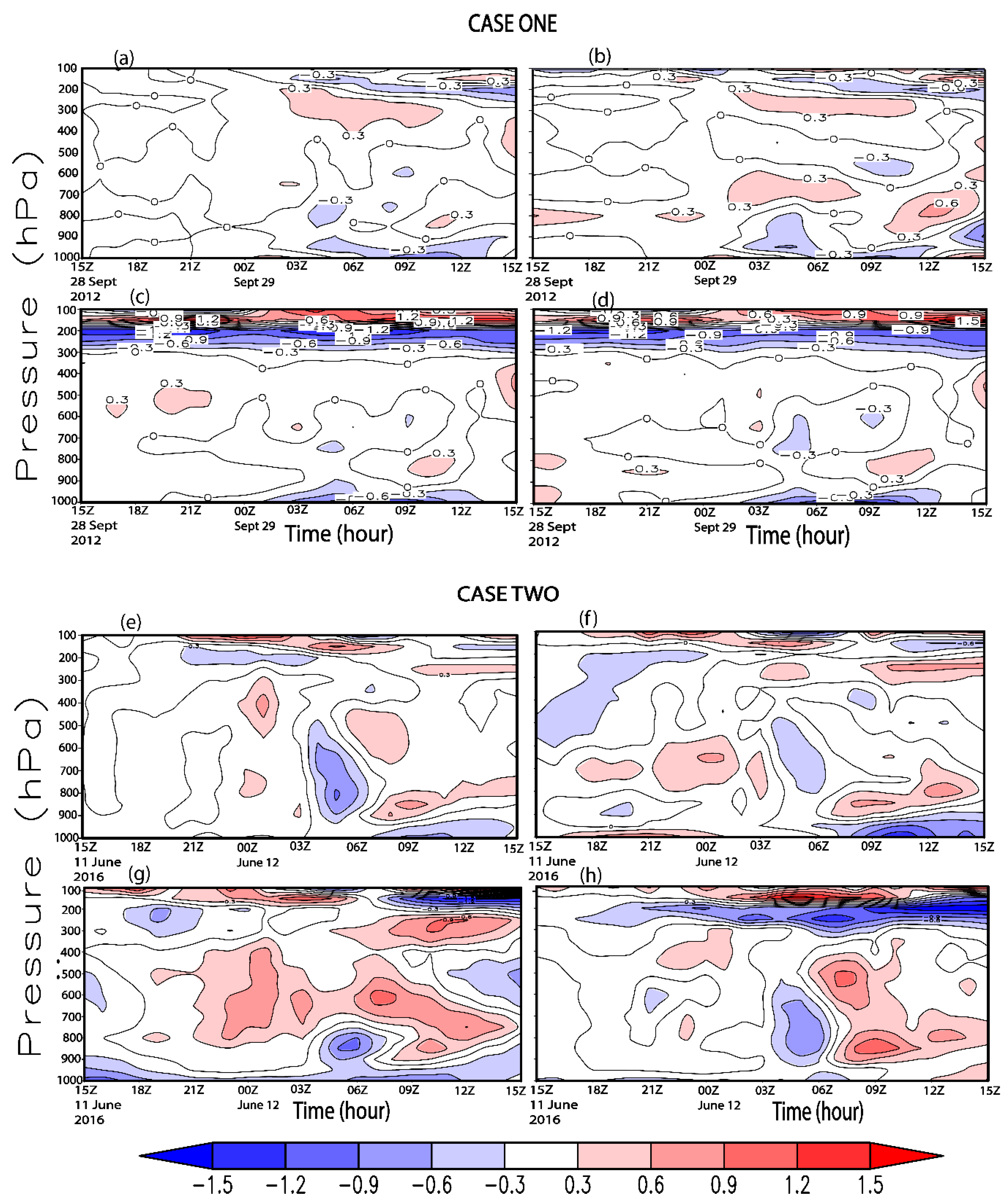
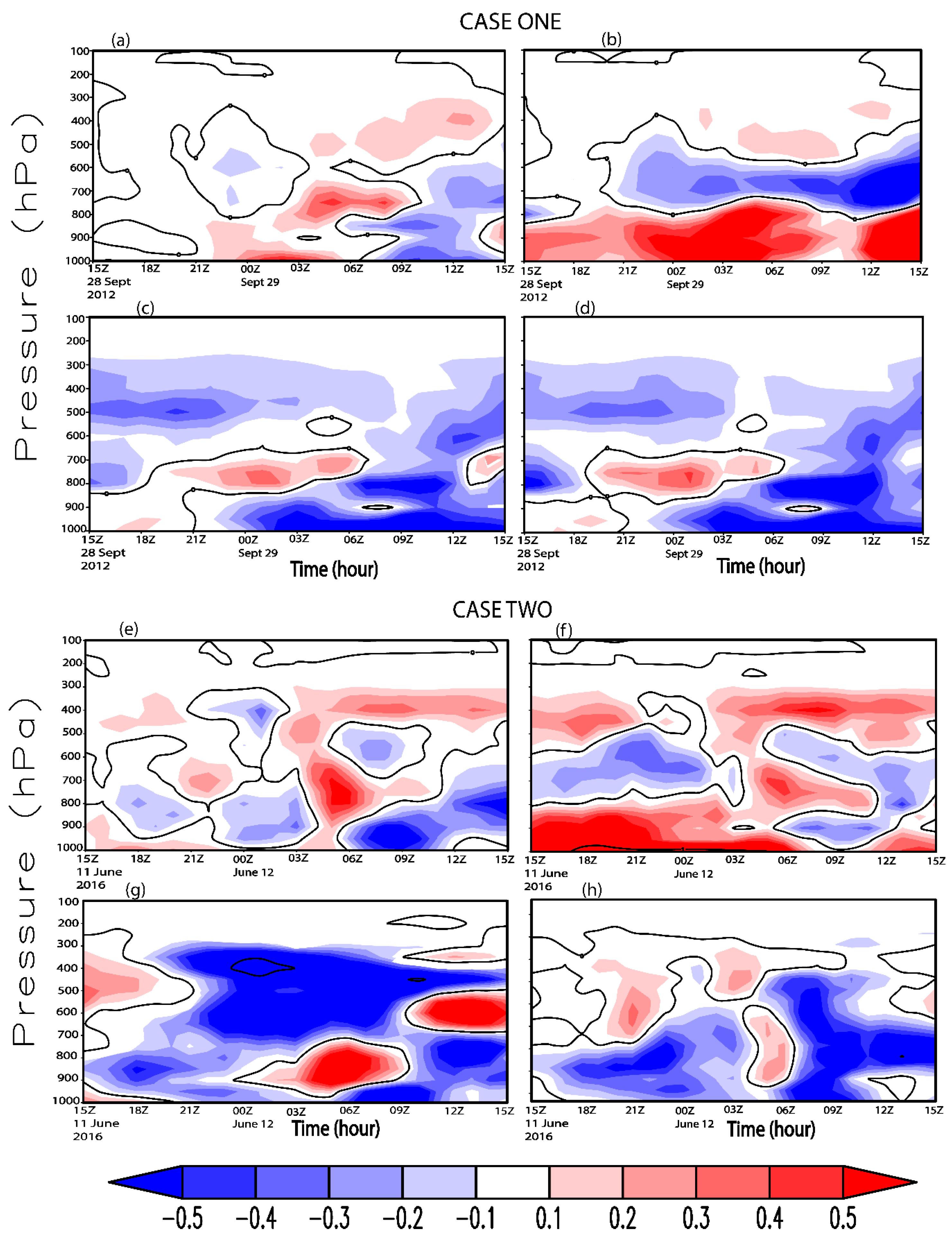
3.2.4. Analysis of the Scheme Simulated Air Temperature and Water Vapor

The ability of the WSM5 scheme in better simulating the highest surface accumulated precipitation than other schemes used for the simulation of the heavy rainfall over the study area is closely examined by considering the air temperature and water vapor simulated by the schemes. The differences between these two variables are plotted and analyzed below. For CASE ONE, Figure 6a shows the difference between air temperature simulated by WSM5 scheme and WSM6 scheme. In the upper troposphere between 200–400 hPa, WSM5 simulated more heating than WSM6. However, CASE TWO scenario given in Figure 6e shows the difference in the value of air temperature simulated by WSM6 and WSM5 schemes. A sizeable number of the heating falls between upper, mid- and lower troposphere of the study area, with some cooling occurring within the mid- to lower tropospheric part. According to reference [21], such heating at that level increases the ice phase particles, which could induce longwave heating. The observed cooling at mid-troposphere could also have been due to enhance ice melting. The resulting increase and decrease in ice-phase particles help to stabilize the large-scale environment that could induce a reduction in local maximum precipitation and its horizontal wide spread distribution. The time-pressure plot of the difference between WSM5 and WDM6 schemes for CASE ONE showed similar characteristics to the plot in Figure 6a. Similarly, a mixture of cooling and heating processes observed in CASE ONE above (Figure 6a) is similar to the CASE TWO as shown in Figure 6f. More heating by WSM5 may have increased ice particles at the upper troposphere but at the mid-troposphere, both heating and cooling are observed with the intensity of the heating being greater than for cooling. We speculated that this could indicate that the ice particles may not have undergone melting at the mid-troposphere thereby reducing the possibilities of converting to precipitation before reaching the surface. The ice particles may have reached the surface in another form rather than precipitation. This could have been responsible for the poor performance of the WDM6 scheme in simulating the surface heavy rainfall. The duo of MORR_G and MORR_H plots for CASE ONE showed that WSM5 simulated enhanced heating at the upper most troposphere (100–200 hPa) and cooling at the (200–300 hPa). The almost nonexistent sufficient heating or cooling at the mid and lower troposphere could have shown that the produced ice particles at the upper troposphere may not have undergone transformation (rimming or aggregation) that lead to the production of precipitation at the surface. However, for CASE TWO, the air temperature plots for the MORR_G and MORR_H schemes shown in Figure 6g,h produced more heating than cooling for MORR_G than in MORR_H scheme in the mid to lower troposphere when compared to CASE ONE. This sufficient heating as well as cooling may have made the performance MORR_G simulate the observed heavy rainfall adequately as it could have enabled the ice particles to undergo sufficient transformation to form rainfall at the surface.
On the other hand, Figure 7a shows the differences in simulated water vapor between WSM5 and WSM6 for CASE ONE. It shows that WSM5 and WSM6 produced almost equal water vapor at the upper-troposphere causing a dry upper atmosphere which means that more water vapor is converted to the ice phase. Similar upper atmosphere dryness is observed in the plot of the differences between WSM5 and WDM6 schemes, as shown in Figure 7b. The same water vapor production between WSM5 and WSM6 schemes were also observed in the CASE TWO shown in Figure 7e as well for the WSM5 and WDM6 schemes shown in Figure 7f showing upper troposphere dryness. However, in the CASE ONE scenario, the observed enhancement of water vapor at the mid-troposphere followed by lower troposphere showed that WSM5 produced less water vapor at the mid-troposphere compared to WDM6 but produced more water vapor at the surface. However for CASE TWO, the intensity of the observed water vapor produced by WSM5 in the mid- troposphere compared to that of WSM6 and WDM6 schemes is lower. This is shown by the mixture of equal proportion of cooling and heating at the mid–and lower troposphere.
The plots for differences between the MORR_G and MORR_H schemes and WSM5 are shown in Figure 7c,d) for CASE ONE. The results show that WSM5 produced less water vapor for consumption to be able to convert it to ice particle at the different levels of the troposphere. The observed heating/dryness at the upper-lower troposphere could be difficult to explain as the in three-dimensional framework because the interactions between each microphysics could result in changes to the large scale environment [19]. Similar results are also obtained for the CASE TWO as shown in Figure 7g,h.

4. Discussion

The advancement in the representation of cloud and precipitation processes in microphysical schemes has provided an opportunity for the modeling and forecasting community to increase accuracy to a higher level in the modeling and forecasting of major physical phenomena like heavy rainfall. However, previous studies [32,33,41,42,43,44] have shown mixed results as to whether microphysical schemes with complex configuration performed better than schemes with a simple configuration. This is so because according to reference [33] the performance of microphysics schemes depends on the climate regimes as well as the targeted phenomena. Therefore, this study was conducted using some selected bulk schemes in WRF model with different ice particles configuration to further highlight this fact by using two reported heavy rainfall events over the southern Nigeria as case studies, while the TRMM rainfall dataset was used for validation purposes only.
The results from CASE ONE showed that WSM5 scheme simulated the highest rainfall amount than other schemes used when compared to TRMM data. Although the WSM5 scheme has been updated to a more complex WSM6 scheme with the addition of a graupel particle, its performance was still below that of the WSM5 in our study. In addition, the performance of WSM6 scheme in simulating better surface accumulated rainfall have also been highlighted e.g., [43,44]. However, our study set out to provide further insights into the role of less dense snow ice particle or dense graupel ice particle in simulating a heavy rainfall event. The maximum rainfall produced by WSM5 could be attributed to the availability of sufficient snow ice particles present in the precipitating cloud that could be converted to rain water directly without further processes (rimming or aggregation) once it passes through the melting point as it falls down. This is a major weakness of the WSM5 scheme and is the main reason why it was updated to WSM6 scheme. Although WSM6 has the second highest amount of simulated rainfall in our study (14.50 mm/day) as can be seen in Table 2, we suggested that its inability to simulate the highest amount of rainfall could be because the precipitating cloud did not possess much of the graupel particle which is the dominant ice particle in the scheme. Furthermore, previous studies e.g., [23,32] have also stated that graupel dominated schemes have shorter cloud residency time resulting into highly localized surface precipitation maximum in both time and space. Also, WSM5 scheme simulated an appropriate amount of longwave heating and less water vapor at upper-, lower-and mid-troposphere, thereby enhancing ice melting processes hence, inducing ice particles to undergo sufficient transformation to form rain water at the surface. This may have been partially responsible for the high amount of rainfall simulated by WSM5 scheme.
On the other hand, CASE TWO study showed that WDM6 scheme gave the highest amount of simulated rainfall than other schemes. Similar results have been obtained in studies involving evaluation of microphysical schemes to simulate warm-type heavy rainfall over Korea Peninsula [33]. The main ice particle in WDM6 scheme is graupel, making it a complex scheme compared to WSM5 scheme in CASE ONE. The WDM6 performance perhaps may be attributed to the possibility of the precipitating cloud having a large number of graupel particles undergoing conversion processes thereby aiding the formation of more rain water at the surface. Also, as stated above, the very short life span of graupel particles make it to rain out quickly leading to the formation of localized maximum precipitation. In addition, the results from both cases about the suitability of hail or graupel in MORR scheme to simulate the heavy rainfall was different. The divergence in the results could be attributed to the densities of these two ice species as well as the complex nature of the MORR scheme in their representation these ice species which is beyond the scope of this present work.
Future studies over the study area would be directed towards using a combination of satellite, radar and in-situ measurement which are presently not available, to validate model simulated outputs to help in improving the model skills for forecasting purposes and other applications. In addition, although mesoscale convective systems are a major mechanism that produce the heavy rainfall such as the type simulated in this study, precipitation can also be localized due to the micro climate of the area favoring such heavy rainfall precipitating. These factors may have an influence on the compositions of ice hydrometeors available in the precipitating cloud. Finally, reference [33] stated that apart from the uncertainty from the microphysics schemes which may have contributed to the difference between the simulated rainfall and observation, other factors like initial conditions and physical processes like land surface or radiation schemes could also have contributed to the forecast errors, but they are not considered in our study.

5. Conclusions

In this study, we have assessed the possible role played by ice hydrometeors in some commonly use bulk microphysics to simulate two reported heavy rainfall events over the southern part of Nigeria during the 2012 and 2016 rainy seasons. The selected bulk schemes used varying categories of ice-phase particles from graupel, hail, ice crystals, and snow aggregates to represent cloud microphysical and precipitation processes. Hence, it makes the selection of the “most appropriate” bulk scheme for weather and climate forecasting over different regions of the world. Therefore, we conducted the study to provide insights into this crucial aspect of weather and climate forecasting using two reported heavy rainfall events over the southern Nigeria as case studies.
Different analyses conducted showed different results for the two heavy rainfall events simulated in this work. In CASE ONE, WSM5 scheme with less dense snow as rime ice particle was able to simulate the accumulated surface rainfall relatively better than others. While in CASE TWO, the WDM6 scheme performed relatively better than other schemes, it underestimated the total surface accumulated rainfall from TRMM. WDM6 contains graupel as its dense rime ice particle. The mixed-phase WSM5 scheme became more complex scheme in WSM6 with the addition of graupel particles as an additional predictive variable. This slow down process in snow and cloud particles direct conversion into rain water may be responsible for WSM6 inability to forecast heavy rainfall as shown in the two cases. In addition, while the WDM6 scheme showed relatively good performance in simulating the surface accumulated in CASE TWO, the major challenge is its inability to simulate correctly the location and perhaps the intensity of the heavy rainfall as shown by the TRMM dataset. Finally, we speculated that the performance of these schemes may also be depended on the various physical mechanisms responsible for the generation of the heavy rainfall. For example, CASE TWO heavy rainfall produced by MCS showed that the WDM6 scheme is almost able to reproduce the total surface accumulated rainfall, which is similar to the result reported by reference [32] in the US Great Plains.
The results from this study have further strengthened the assertion by reference [16] that complex microphysical schemes do not necessarily perform better than simple schemes. Furthermore, it shows that the representation of clouds and precipitation processes in mesoscale numerical models is still not perfect especially in bulk schemes, while considerable improvement has been achieved with bin microphysics schemes which cannot still be used in weather and climate forecasting due to the huge computational resources required.
Based on the above facts, there is a need for weather forecasters in different regions of the world to evaluate different microphysical schemes used in mesoscale forecast models for different meteorological phenomena and its associated dynamics producing such phenomena in their region. This would help in the selection of a more appropriate bulk scheme for simulating such phenomena.

Author Contributions

This study was conceived, planned and designed by O.E.A. All simulations, calculations, data analysis and manuscript drafting was done by O.E.A. and was reviewed, modified and approved by Y.Y.

Acknowledgments

This work was supported by grants from the National Natural Science Foundation of China (41590873). Era-interim datasets used were sourced from ECMWF (https://apps.ecmwf.int/datasets/data/interim-full-daily) and TRMM rainfall dataset from NASA (http://mirador.gsfc.nasa.gov/). The authors also thank NCAR for making the WRF model software available free of charge for use in this work. The first author is grateful to the Federal Republic of Nigeria through the Tertiary Education Trust Fund (TETFUND) for providing funding for his PhD degree and also to the Obafemi Awolowo University, Ile-Ife, Nigeria for granting the study leave to undertake the program. The high performing computer (HPC) used for this work is provided by the Nanjing University of Information Science and Technology, Nanjing, China. The comments and suggestions provided by the three anonymous reviewers and academic editor to improve the earlier version of the manuscript are highly appreciated.

Conflicts of Interest

The authors declare no conflict of interest.

References

  1. Omotosho, J.B. The separate contributions of line squalls, thunderstorms and the monsoon to the total rainfall in Nigeria. J. Climatol. 1985, 5, 543–552. [Google Scholar] [CrossRef]
  2. Panthou, G.; Vischel, T.; Lebel, T.; Blanchet, J.; Quantin, G.; Ali, A. Extreme rainfall in West Africa: A regional modeling. Water Resour. Res. 2012, 48, W08501. [Google Scholar] [CrossRef]
  3. Agada, S.; Nirupama, N. A serious flooding event in Nigeria in 2012 with specific focus on Benue State: A brief review. Nat. Hazards 2015, 77, 1405–1414. [Google Scholar] [CrossRef]
  4. Nkwunonwo, U.C.; Malcolm, W.; Brian, B. Flooding and Flood Risk Reduction in Nigeria: Cardinal Gaps. J. Geogr. Nat. Disaster 2015, 5, 136. [Google Scholar] [CrossRef]
  5. Ubachukwu, N.N.; Emeribe, C.N. The 2012 flooding in selected parts of Isoko South, Delta State: Assessment of Soico-Economic Impacts, Mediterranean. Mediterr. J. Soc. Sci. 2017, 8, 353–358. [Google Scholar] [CrossRef]
  6. Babatolu, J.S.; Akinnubi, R.T.; Folagimi, A.T.; Bukola, O.O. Variability and Trends of Daily Heavy Rainfall Events over Niger River Basin Development Authority Area in Nigeria. Am. J. Clim. Chang. 2014, 3, 1–7. [Google Scholar] [CrossRef] [Green Version]
  7. Egbebiyi, T.S. Future Changes in Extreme Rainfall Events and African Easterly Waves over West Africa. Master’s Thesis, Department of Environmental and Geographical Science, University of Cape Town, Cape Town, South Africa, 2016, unpublished. [Google Scholar]
  8. Bouniol, D.; Dalanoe, J.; Duroure, C.; Protat, A.; Giraud, V.; Penide, G. Microphysical characterization of West African MCS anvils. Q. J. R. Meteorol. Soc. 2010, 136, 323–344. [Google Scholar] [CrossRef]
  9. Dione, C.; Lohou, F.; Lothon, M.; Adler, B.; Babić, K.; Kalthoff, N.; Pedruzo-Bagazgoitia, X.; Bezombes, Y.; Gabella, O. Low Level Cloud and Dynamical Features within the Southern West African Monsoon. Atmos. Chem. Phys. Discuss. 2018. [Google Scholar] [CrossRef]
  10. Adler, B.; Babić, K.; Kalthoff, N.; Lohou, F.; Lothon, M.; Dione, C.; Pedruzo-Bagazgoitia, X.; Andersen, H. Nocturnal low-level clouds in the atmospheric boundary layer over southern West Africa: An observation-based analysis of conditions and processes. Atmos. Chem. Phys. Discuss. 2018, 2018, 1–31. [Google Scholar] [CrossRef]
  11. Ibrahim, S.; Afandi, G. Short-range Rainfall Prediction over Egypt using the Weather Research and Forecasting Model. Open J. Renew. Energy Sustain. Dev. 2014, 2014, 56–70. [Google Scholar] [CrossRef]
  12. Akinsanola, A.A.; Aroninuola, B.A. Diagnostic Evaluation of September 29, 2012 Heavy Rainfall Event over Nigeria. J. Climatol. Weather Forecast. 2016, 4, 155. [Google Scholar] [CrossRef]
  13. Diongue, A.; Lafore, J.-P.; Redelsperger, J.-L.; Roca, R. Numerical study of a Sahara synoptic weather system: Initiation and mature stages of convection and its interactions with the large-scale dynamics. Q. J. R. Meteorol. Soc. 2002, 128, 1899–1927. [Google Scholar] [CrossRef]
  14. Maranan, M.; Fink, A.H.; Knippertz, P.; Francis, S.D.; Akpo, A.B.; Jegede, G.; Yorke, C. Interactions between Convection and a Moist Vortex Associated with and Extreme Rainfall Event over Southern Africa. Mon. Weather Rev. 2019, 147, 2309–2328. [Google Scholar] [CrossRef]
  15. Hou, A.Y.; Kakar, R.K.; Neeck, S.; Azarbarzin, A.A.; Kummerow, C.D.; Kojima, M.; Oki, R.; Nakamura, K.; Iguchi, T. The global precipitation measurement mission. Bull. Am. Meteorol. Soc. 2014, 95, 701–722. [Google Scholar] [CrossRef]
  16. Straka, J.M. Cloud and Precipitation Microphysics: Principle and Parameterizations; Cambridge University Press: New York, NY, USA, 2009; p. 392. [Google Scholar]
  17. Hong, S.-Y. Comparison of heavy rainfall mechanisms in Korea and the central US. J. Meteorol. Soc. Jpn. Ser. II 2004, 82, 1469–1479. [Google Scholar] [CrossRef]
  18. Akinbobola, A.; Okogbue, E.C.; Ayansola, A.K. Statistical Modeling of Monthly Rainfall in Selected Stations in Forest and Savannah Eco-climatic Regions of Nigeria. J. Climatol. Weather Forecast. 2018, 6, 226. [Google Scholar] [CrossRef]
  19. Hong, S.-Y.; Dudhia, J.; Chen, S.-H. A revised approach to ice microphysical processes for the bulk parameterization of clouds and precipitation. Mon. Weather Rev. 2004, 132, 103–120. [Google Scholar] [CrossRef]
  20. Hong, S.-Y.; Lim, J.-O.J. The WRF single-moment 6-class microphysics scheme (WSM6). J. Korean Meteorol. Soc. 2006, 42, 129–151. [Google Scholar]
  21. Lim, K.-S.S.; Hong, S.-Y. Development of an effective double moment cloud microphysics scheme with prognostic cloud condensation nuclei (CCN) for weather and climate models. Mon. Weather Rev. 2010, 138, 1587–1612. [Google Scholar] [CrossRef]
  22. Morrison, H.; Thompson, G.; Tatarskii, V. Impact of cloud microphysics on the development of trailing stratiform precipitation in a simulated squall line: Comparison of one-and two-moment schemes. Mon. Weather Rev. 2009, 137, 991–1007. [Google Scholar] [CrossRef]
  23. Hong, S.-Y.; Noh, Y.; Dudhia, J. A new vertical diffusion package with an explicit treatment of entrainment processes. Mon. Weather Rev. 2006, 134, 2318–2341. [Google Scholar] [CrossRef]
  24. Kain, J.S. The Kain-Fritsch convective parameterization: An update. J. Appl. Meteorol. 2004, 43, 170180. [Google Scholar] [CrossRef]
  25. Mlawer, E.J.; Taubman, S.J.; Brown, P.D.; Iacono, M.J.; Clough, S.A. Radiative transfer for inhomogeneous atmosphere: RRTM, a validated correlated-k model for the longwave. J. Geophys. Res. 1997, 102, 16663–16682. [Google Scholar] [CrossRef]
  26. Dudhia, J. Numerical study of convection observed during the Winter Monsoon Experiment using mesoscale two-dimensional model. J. Atmos. Sci. 1989, 46, 3077–3107. [Google Scholar] [CrossRef]
  27. Chen, F.; Dudhia, J. Coupling an advanced land surface–hydrology model with the Penn State–NCAR MM5 modeling system. Part I: Model implementation and sensitivity. Mon. Weather Rev. 2001, 129, 569–585. [Google Scholar] [CrossRef]
  28. Huffman, G.J.; Bolvin, D.T.; Nelkin, E.J.; Wolff, D.B.; Adler, R.F.; Gu, G.; Hong, Y.; Bowman, K.P.; Stocker, E.F. The TRMM Multisatellite Precipitation Analysis (TMPA): Quasi-Global, Multiyear, Combined-Sensor Precipitation Estimates at Fine Scales. J. Hydrometeorol. 2007, 8, 38–55. [Google Scholar] [CrossRef]
  29. Gbode, I.E.; Dudhia, J.; Ogunjobi, K.O.; Ajayi, V.O. Sensitivity of different physics schemes in the WRF model during a West African monsoon regime. Theor. Appl. Climatol. 2018, 136, 733–751. [Google Scholar] [CrossRef] [Green Version]
  30. Tanessong, R.S.; Vondou, D.A.; Djomou, Z.Y.; Igri, P.M. WRF high resolution simulation of an extreme rainfall event over Douala (Cameroon): A case study. Model. Earth Syst. Environ. 2017, 3, 927–942. [Google Scholar] [CrossRef]
  31. Jones, P.W. First- and Second-Order Conservative Remapping Schemes for Grids in Spherical Coordinates. Mon. Weather Rev. 1999, 127, 2204–2210. [Google Scholar] [CrossRef]
  32. Pu, Z.; Lin, C.; Dong, X.; Krueger, K.S. Sensitivity of Numerical Simulations of a Mesoscale Convective System to Ice Hydrometeors in Bulk Microphysical Parameterization. Pure Appl. Geophys. 2018, 176, 2097–2120. [Google Scholar] [CrossRef]
  33. Song, H.-J.; Sohn, B.-J. An Evaluation of WRF microphysics Schemes for Simulating the Warm-Type Heavy Rain over the Korean Peninsula. Asia Pac. J. Atmos. Sci. 2018, 54, 225–236. [Google Scholar] [CrossRef]
  34. Hong, S.-Y.; Lim, K.-S.S.; Lee, Y.-H.; Ha, J.-C.; Kim, H.-W.; Ham, S.-J.; Dudhia, J. Evaluation of the WRF double-moment 6-class microphysics scheme for precipitating convection. Adv. Meteorol. 2010, 2010, 707253. [Google Scholar] [CrossRef]
  35. Ite, A.E.; Ibok, U.J. Gas Flaring and Venting Associated with Petroleum Exploration and Production in the Nigeria’s Niger Delta. Am. J. Environ. Prot. 2013, 1, 70–77. [Google Scholar] [CrossRef]
  36. Giwa, S.O.; Adama, O.O.; Akinyemi, O.O. Baseline black carbon emissions for gas flaring in the Niger Delta region of Nigeria. J. Nat. Gas Sci. Eng. 2014, 20, 373–379. [Google Scholar] [CrossRef]
  37. Towney, S. Pollution and the planetary albedo. Atmos. Environ. 1974, 8, 1251–1256. [Google Scholar]
  38. Albrecht, B.A. Aerosols, cloud microphysics, and fractional cloudiness. Science 1989, 245, 1227–1231. [Google Scholar] [CrossRef] [PubMed]
  39. Song, H.-J.; Sohn, B.-J.; Hong, S.-Y.; Hashino, T. Idealized numerical experiments on the microphysical evolution of warm-type heavy rainfall. J. Geophys. Res. 2017, 122, 1685–1699. [Google Scholar] [CrossRef]
  40. Houze, R.A.; Biggerstaff, M.I.; Rutledge, S.A.; Smull, B.F. Interpretation of Doppler weather radar displays of midlatitude mesoscale convective systems. Bull. Am. Meteorol. Soc. 1989, 70, 608–619. [Google Scholar] [CrossRef]
  41. Efstathiou, G.A.; Zoumakis, N.M.; Melas, D.; Kassomenos, P. Imapct of Precipitating Ice on the Simulation of a Heavy Rainfall Event with Advanced Research WRF using Two Bulk Microphysics Schemes. Asia Pac. J. Atmos. Sci. 2012, 48, 357–368. [Google Scholar] [CrossRef]
  42. Van Weverberg, K.; Vogelmann, A.M.; Lin, W.; Luke, E.P.; Cialella, A.; Minnis, P.; Khaiyer, M.; Boer, E.R.; Jensen, M.P. The role of cloud microphysics parameterization in the simulation of mesoscale convective system clouds and precipitation in the tropical western Pacific. J. Atmos. Sci. 2013, 70, 1104–1128. [Google Scholar] [CrossRef]
  43. Wu, D.; Dong, X.; Xi, B.; Feng, Z.; Kennedy, A.; Mullendore, G.; Gilmore, M.; Tao, W.-K. Impacts of microphysical scheme on convective and stratiform characteristics in two high precipitation squall line events. J. Geophys. Res. Atmos. 2013, 118, 11119–11135. [Google Scholar] [CrossRef]
  44. Kar, S.C.; Tiwari, S. Model simulations of heavy precipitation in Kashmir, India, in September 2014. Nat. Hazards 2016, 81, 167–188. [Google Scholar] [CrossRef]
Figure 1. (a) Topographical map showing the simulation nested domains (b) The enlarged. inner red rectangle (5° E–9° E, 4° N–6° N) shows the area analyzed in this study.
Atmosphere 10 00513 g001
Figure 2. (a) Geopotential Height (m) (blue solid contour) at 850 hPa with wind speed (m/s) at 500 hPa level (overlaid) (b) Mean Sea Level Pressure (yellow solid contour) at 850 hPa level and wind speed (m/s) at 500 hPa level (overlaid) over the West Africa region at 06Z 28-09-2012 (CASE ONE). (c) Geopotential Height (m) (blue solid contour) at 850 hPa with wind speed (m/s) at 500 hPa level (overlaid) (d) Mean Sea Level Pressure (yellow solid contour) at 850 hPa level and wind speed (m/s) at 500 hPa level (overlaid) at 06Z 11-06-2016 (CASE TWO).
Atmosphere 10 00513 g002
Figure 3. Spatial distributions of 24 h accumulated rainfall in mm over the study area with plot of CASE ONE. (a) TRMM data (b) MORR_G (c) MORR_H (d) WDM6 (e) WSM6 (f) WDM5 and CASE TWO (g) TRMM data (h) MORR_G (i) MORR_H (j) WDM6 (k) WSM6 and (l) WSM5.
Atmosphere 10 00513 g003
Figure 4. Area average (5 °N–9 °E, 4 °N–6 °N) of vertical profile distribution of mass mixing ratio for CASE ONE (a) cloud (b) snow (c) graupel/hail (d) rain and (e) ice and CASE TWO (f) cloud (g) snow (h) graupel/hail (i) rain and (j) ice.
Atmosphere 10 00513 g004
Figure 5. Time series of area–averaged (5° N–9° E, 4° N–6° N) hydrometeors paths of all the schemes used and their cloud hydrometeors CASE ONE (a) MORR_G (b) MORR_H (c) WDM6 (d) WSM6 and (e) WSM5 and CASE TWO (f) MORR_G (g) MORR_H (h) WDM6 (i) WSM6 and (j) WSM5.
Atmosphere 10 00513 g005
Figure 6. Pressure-time cross sections of the differences in air temperature (K) CASE ONE (a) WSM5–WSM6 (b) WSM5–WDM6 (c) WSM5–MORR_G and (d) WSM5–MORR_H and CASE TWO (e) WSM–WSM6 (f) WSM5–WDM6 (g) WSM5–MORR_G and (h) WSM5–MORR_H averaged over the heavy rainfall region (5° N–9° E, 4° N–6° N).
Atmosphere 10 00513 g006
Figure 7. Pressure-time cross sections of the differences in water vapor (g/kg) between CASE ONE (a) WSM5–WSM6 (b) WSM5–WDM6 (c) WSM5–MORR_G and (d) WSM5–MORR_H and CASE TWO (e) WSM –WSM6 (f) WSM5–WDM6 (g) WSM5–MORR_G and (h) WSM5–MORR_H averaged over the heavy rainfall region (5° N–9° E, 4° N–6° N).
Atmosphere 10 00513 g007
Table 1. Mass mixing ratio and number concentration of variables used in the study.
Bulk Scheme NameMass Mixing Ratio Prognosis VariablesNumber Mixing Ratio Prognosis Variables
WSM5Qr Qc Qi Qs
WSM6Qr Qc Qi Qs Qg
WDM6Qr Qc Qi Qs QgNn Nc Nr
MORR -2 momentQr Qc Qi Qs QgNr Nr Nc Ng
c = cloud, r = rain, i = ice, s = snow, g = graupel, Q = mixing ratio, N = number concentration and Nn = CCN number.
Table 2. Results of statistical metrics used to validate the model simulated accumulated rainfall with TRMM datasets.
CASE ONECASE TWO
TRMMMORR_GMORR_HWDM6WSM6WSM5TRMMMORR_GMORR_HWDM6WSM6WSM5
Accumulated Rainfall (mm/day)22.2314.0313.6813.6714.5017.3214.5717.2727.5815.1421.4029.18
Mean Bias (mm/day) 8.208.558.567.734.91 −2.70−13.01−0.58−6.82−14.61
RMSE (mm/day) 2.903.023.032.731.74 0.964.600.22.415.16

