Article

Characteristics of Ozone Pollution, Regional Distribution and Causes during 2014–2018 in Shandong Province, East China

1
College of Geography and Environment, Shandong Normal University, Ji’nan 250014, China
2
Institute of Information Science and Technology, Shandong Normal University, Ji’nan 250014, China
3
Shandong Province Environment Information and Monitoring Center, Ji’nan 250101, China
4
Center for Environmental Technology and Policy Research, Shandong Normal University, Ji’nan 250014, China
*
Author to whom correspondence should be addressed.
Atmosphere 2019, 10(9), 501; https://doi.org/10.3390/atmos10090501
Submission received: 18 July 2019 / Revised: 7 August 2019 / Accepted: 23 August 2019 / Published: 27 August 2019
(This article belongs to the Section Air Quality)

Abstract

:
The summer ozone pollution of Shandong province has become a severe problem in the period 2014–2018. Affected by the monsoon climate, the monthly average ozone concentrations in most areas were unimodal, with peaks in June, whereas in coastal areas the concentrations were bimodal, with the highest peak in May and the second highest peak in September. Using the empirical orthogonal function method, three main spatial distribution patterns were found. The most important pattern proved the influences of solar radiation, temperature, and industrial structure on ozone. Spatial clustering analysis of the ozone concentration showed Shandong divided into five units, including Peninsula Coastal area (PC), Lunan inland area (LN), Western Bohai area (WB), Luxi plain area (LX), and Luzhong mountain area (LZ). Influenced by air temperature and local circulation, coastal cities had lower daytime and higher nighttime ozone concentrations than inland. Correlation analysis suggested that ozone concentrations were significantly positively correlated with solar radiation. The VOCs from industries or other sources (e.g., traffic emission, petroleum processing, and chemical industries) had high positive correlations with ozone concentrations, whereas NOx emissions had significantly negatively correlation. This study provides a comprehensive understanding of ozone pollution and theoretical reference for regional management of ozone pollution in Shandong province.

1. Introduction

Ozone is a common air pollutant in the boundary layer. It is formed by photochemical reactions of volatile organic compounds (VOCs) and nitrogen oxides (NOx) under sufficient light conditions [1,2]. Sedimentation from stratospheric and cross-regional transport are also important sources of ground-level ozone [3]. As an extremely strong oxidant, ozone can regulate the life of chemical and climate-related trace materials by affecting their oxidation processes in the troposphere [4]. Long-term exposure to high ozone concentrations not only affects food crops but also increases the risk of death by damaging the respiratory and cardiovascular systems of the human body [5,6,7]. Moreover, ozone is regarded as the third-largest anthropogenic greenhouse gas [8]. Industrialization and urbanization have resulted in China’s ozone pollution becoming increasingly serious [9]. In certain areas, ozone has even replaced PM2.5 as the primary pollutant [10]. Due to its impacts on climate change, air quality, and human health, ground-level ozone is a cause of widespread concern.
In recent years, numerous studies have focused on ozone pollution in eastern China, especially in the Beijing–Tianjin–Hebei (BTH), Yangtze River Delta (YRD), and Pearl River Delta (PRD) [11,12,13]. In addition to regional studies, studies of urban ozone have also been reported, such as Wuhan, Chengdu, and Zhengzhou [14,15,16]. These studies discussed issues including the temporal and spatial distribution of ozone pollution, source and process analysis, meteorological conditions, and pollution control measures.
Shandong province is bordered by the BTH region in the north and has the second-largest population and the third-largest gross domestic product (GDP) in China by 2017. It is also one of the regions with the highest levels of pollutant emissions and air pollution in China [17]. In recent years, most studies on air pollution have focused on fine particulate matter (aerosols) and mixed pollutants [17,18,19]. Local ozone pollution has also been studied in a few areas such as Jinan (JNA), Qingdao (QD), and Mount Tai [20,21,22]. The ozone pollution in Shandong province shows an increasing trend [23], so it is necessary to study the characteristics of ozone pollution in Shandong province.
The ground-level ozone concentration is closely related to meteorological conditions [24]. For example, the wind cycle changes the transportation and accumulation of ozone [25], and solar radiation and temperature affect the biological emissions and reaction rates of the precursors [26]. It is generally believed that high temperatures, static wind, low cloud, high solar radiation, low humidity, and static weather are conducive to ozone pollution [27]; solar radiation is regarded as the particularly decisive factor for the formation of ground-level ozone [28]. In addition, local circulation by wind from valleys and sea–land breeze has also proved to be an important dynamic feature influencing ozone concentration [4]. Differences in meteorological conditions will result in different spatial and temporal distributions of ozone concentrations in different cities in one region, as confirmed in the BTH, YRD, and PRD [29,30,31].
Moreover, VOCs and NOx emitted by transportation and industries are the main sources of ground-level ozone pollution [32,33]. Solvent use and industrial processes are considered to be the main sources of VOCs in China, with the five major industries of plastics products, rubber products, chemical fiber products, the chemical industry, and oil refining accounting for 70% of industrial emissions [34]. Manufacturing, electricity production, and transportation together account for approximately 90% of the national NOx emissions [35]. Due to the complex generation mechanisms of ozone (VOC and NOx-limited), the relationship between urban ozone concentration and specific industries remains unclear [3].
Based on the characteristics of ozone concentrations from 2014–2018, this study explored the spatial distribution types of ozone pollution in Shandong province using the empirical orthogonal function (EOF) and cluster analysis method. The effects of meteorological conditions and industries on ozone pollution in different regions of Shandong province are also discussed. This study aims to address the following issues:
  • What were the temporal and spatial characteristics of ozone pollution in Shandong province during 2014–2018, and changes in the types of spatial distribution of ozone pollution?
  • How do meteorological factors affect ozone pollution in Shandong province?
  • What are the impacts of industrial structure and traffic on ozone pollution in Shandong province?

2. Methods

2.1. Study Area

Shandong province (34°22.9′ N–38°24.01′ N, 114°47.5′ E–122°42.3′ E) is in the east of the North China Plain and downstream of the Yellow River (Figure 1). Shandong is north of China’s political center (the BTH region) and south of China’s economic center (the YRD). It is roughly divided into an eastern peninsula area (bordering the Bohai Sea and the Yellow Sea and closing to the Liaodong Peninsula); central hilly area; and northern and southwestern plain areas. With a monsoon season and warm temperate climate of middle latitudes, precipitation and heat in Shandong province are concentrated in summer, and their seasonal variations are simultaneous. The prevailing wind directions are southeast in spring and summer, and northwest in autumn and winter [17,18]. As of 2017, the total population of the province exceeds 100 million and the population density was as high as 634 people per square kilometer. With several types of industries, the GDP of Shandong is the third highest in China. Shandong province is generally located in a relatively closed geographical unit surrounded by Yanshan, Taihang, and Dabie mountain, which is not conducive to the diffusion of air pollutants, therefore this region is one of the most heavily polluted areas in China [17]. The main air pollutants in the region are particulate matter (mainly in winter and spring) and ground-level ozone (mainly in summer).

2.2. Data Collection

The air quality data used in this study were from routine monitoring data of national and provincial environmental air quality monitoring stations (a total of 154; Figure 1), which are all located in urban areas (built-up area severely affected by humans) and suburban areas (non-built area that is less affected by humans and can be regarded as background points partly) [17]. Meteorological data were obtained from the National Meteorological Information Center (http://data.cma.cn/site/index.html). Total solar radiation data were obtained from the National Meteorological Center, based on observations such as ground sunshine hours, and estimated using the Hybrid model. All economic and social data were derived from the Shandong statistical yearbook of 2015–2018 or the statistical yearbooks of various cities.

2.3. Analytical Methods

To acquire the initial value and the number of clusters to be used in cluster analysis, the EOF was used to determine the characteristic distribution of ozone concentrations. The central station for cluster analysis was determined according to the pattern with the largest contribution rate of variance [36].

2.3.1. Empirical Orthogonal Function (EOF)

The EOF, also known as eigenvector analysis, is a method of analyzing structural features in matrix data and extracting the main feature quantities. This analysis can decompose the variable field with time into the spatial function, which does not change with time, and the time function that depends only on time variation. It has been widely used in the fields of meteorology, climate and ocean research [37], and has also been applied to investigate the temporal and spatial characteristics of ozone pollution, such as the 1980–2010 summers in the eastern United States and 2014 in eastern China [38,39].

2.3.2. Cluster Analysis Method

Based on the results of EOF analysis, cluster analysis was carried out on 154 monitoring stations in Shandong province. The center point and the number of clusters were determined by the feature field with the largest variance contribution, and the k-mean cluster was used for division. This method has also been widely used in the analysis of the temporal and spatial distribution of ozone pollution, e.g., the cluster analysis was used to divide Seville’s ozone pollution into suburban areas, urban areas and the monitoring area used for transportation emissions by Pavón-Domínguez [40].

3. Results

3.1. Time Feature

3.1.1. Annual Variation

The annual average hourly ozone concentration, annual maximum daily 8 h average (MDA8) ozone concentration, and 90th percentile of MDA8 in Shandong province from 2014–2018 were calculated (Table 1). The indicators all reflected an increasing trend in ozone pollution, with growth rates of 19.96%, 18.88% and 15.10%, respectively. The highest growth rates of 9.24%, 8.61% and 7.93% for the annual average hourly ozone concentration, MDA8 ozone concentration, and 90th percentile of MDA8 were observed in 2017 comparable to 2016.
Table 1 compares the ozone concentration in Shandong province with other developed regions. The results showed that ozone pollution in Shandong was slightly lower than in the BTH but higher than in the YRD and PRD and the average concentration in the central and eastern regions of China. Unlike in the YRD and PRD, the ozone concentration in Shandong province has maintained a year-on-year growth trend.
Figure S1 shows the annual average ozone concentration changes in 17 cities in Shandong in 2014–2018. The fluctuations in most regions, especially in Binzhou (BZ), Liaocheng (LC), Laiwu (LW, merged into Jinan in 2019), and Tai’an (TA), show an increasing tendency. The ozone concentration exceeding the Chinese standard for 17 cities in Shandong was calculated (Figure S2). The result showed that except for Weihai (WH), Weifang (WF) and Zaozhuang (ZZ), the ozone over-standard rate in other regions continued to rise, while BZ, LW, and LC increased significantly. The World Health Organization guideline level for ozone is 100 μg/m3 (daily MDA8) and ten cities in Shandong exceeded it for more than 200 days in 2018 (Figure S2). Compared with the data from other areas of China in 2015 and 2016, the situation in Shandong province is more serious than that in the central and eastern regions of China, the PRD, or Beijing [41,42].

3.1.2. Monthly Variation

The monthly average ozone concentration in 2014–2018 showed that the annual variation in ozone concentration in most inland areas of Shandong was unimodal (Figure 2). The peak appeared in June and the valley was in December or January. Coastal areas such as WH showed a bimodal trend, with the highest concentration in May and the second highest concentration in September.
The annual variation in the ozone concentration was influenced by climatic conditions. Most inland areas of Shandong are affected by the summer monsoon and subtropical anticyclone in June, with higher temperatures, lower humidity, and cloud over compared with July and August, which is conducive to the formation of ground-level ozone. In July and August, Shandong province is affected by the warm moist southerly winds from the ocean, so that cloud cover and precipitation increase considerably [43], and ozone production is limited. For the coastal area, due to the influence of the sea breeze, the highest temperature in summer is lower than in inland areas. In addition, the increased precipitation from June to August results in lower coastal temperatures than in inland areas. Therefore, the low concentrations of ozone were observed in coastal cities. With the subtropical high and monsoon retreating in September, cloud cover and humidity decreased, and the ozone concentration in inland areas decreased; however, ozone short-term pollution process may occur during rare high-temperature events. The ozone concentration of the coastal area showed a second peak in September. After October, with the solar radiation intensity and temperature decreasing, the ozone concentration was the lowest in winter.
Studies in other regions have also confirmed the impact of monsoon on ozone concentrations. The ozone concentrations in Beijing, the YRD, and Wuhan are all unimodal [14,44,45]. Similar to the situation in Shandong province, the peak concentrations in Beijing and the YRD occurred prior to impacts of the monsoon, while the peak concentration in Wuhan occurred after the monsoon. As for Guangxi Province in China and the Indian peninsula, which are located at low latitudes and have high temperatures throughout most of the year, have obvious bimodal types, with peaks appearing both before and after the impacts of monsoon [46,47].

3.1.3. Diurnal Variation

The ozone concentration in Shandong province was unimodal (Figure 3). The lowest concentration appeared between 6 and 7 am due to the weak process of precursor conversion to ozone at nighttime and the strong ozone depletion effect caused by NO titration and dry sedimentation [48,49]. During the daytime, the increase in precursor emissions, temperature and solar radiation results in the photolysis of NO2 dominating O3–VOC–NOx chemistry [50], which leads to an increase in the ground-level ozone concentration and a peak between 3 and 4 pm. Similar daily changes in ozone concentrations have been observed in Beijing, the YRD, India and Europe [30,42,51,52].
The nighttime ozone concentrations in coastal cities of Shandong province (WH, QD, YT, and RZ) were considerably higher than those in inland areas, while daytime ozone peaks were relatively low, and the daily disparity was much smaller than in inland areas. A similar situation was observed in Northern Europe [53], which was related to the differences in meteorological conditions between coastal and inland cities.

3.2. Spatial Characteristics

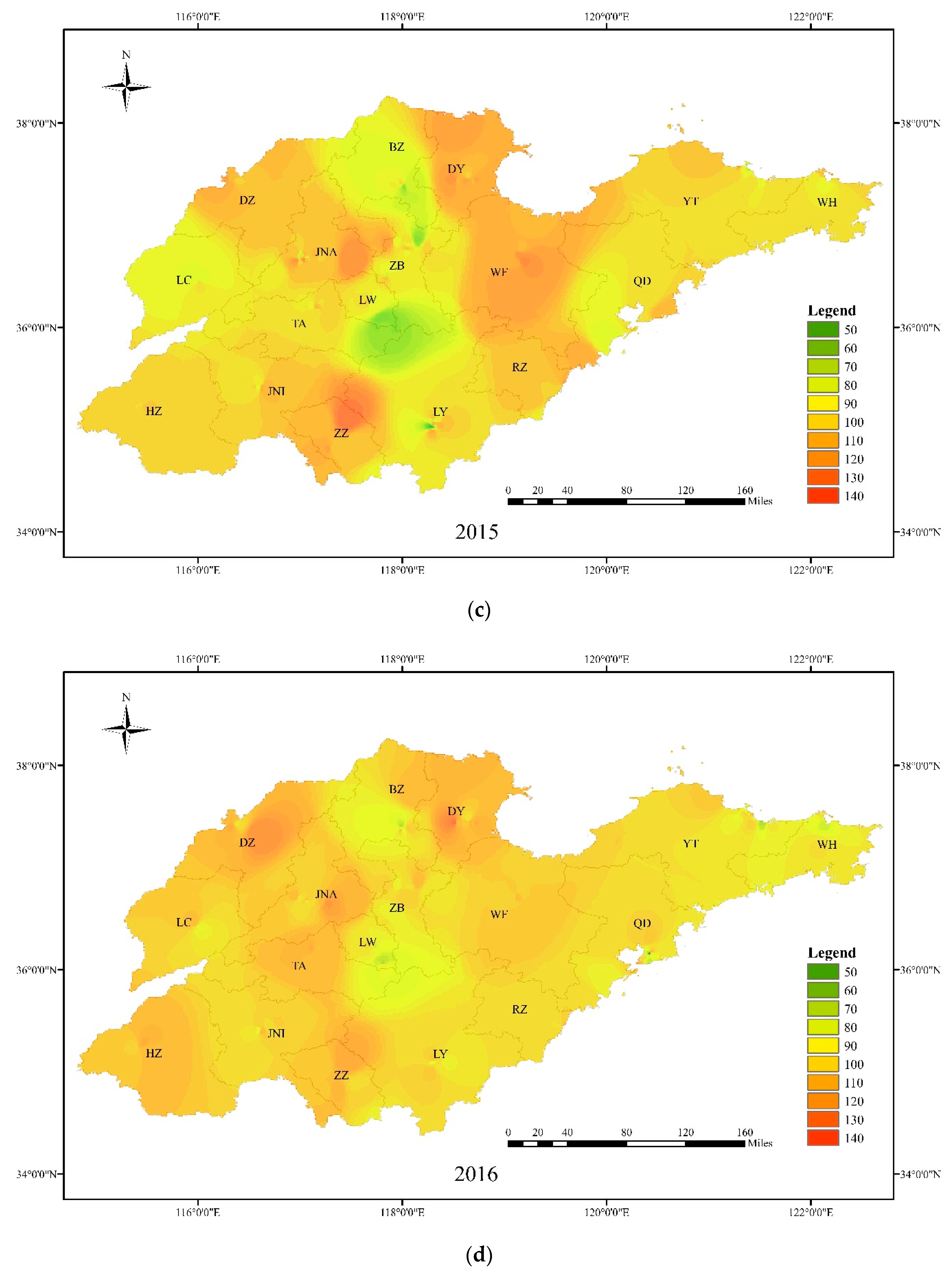
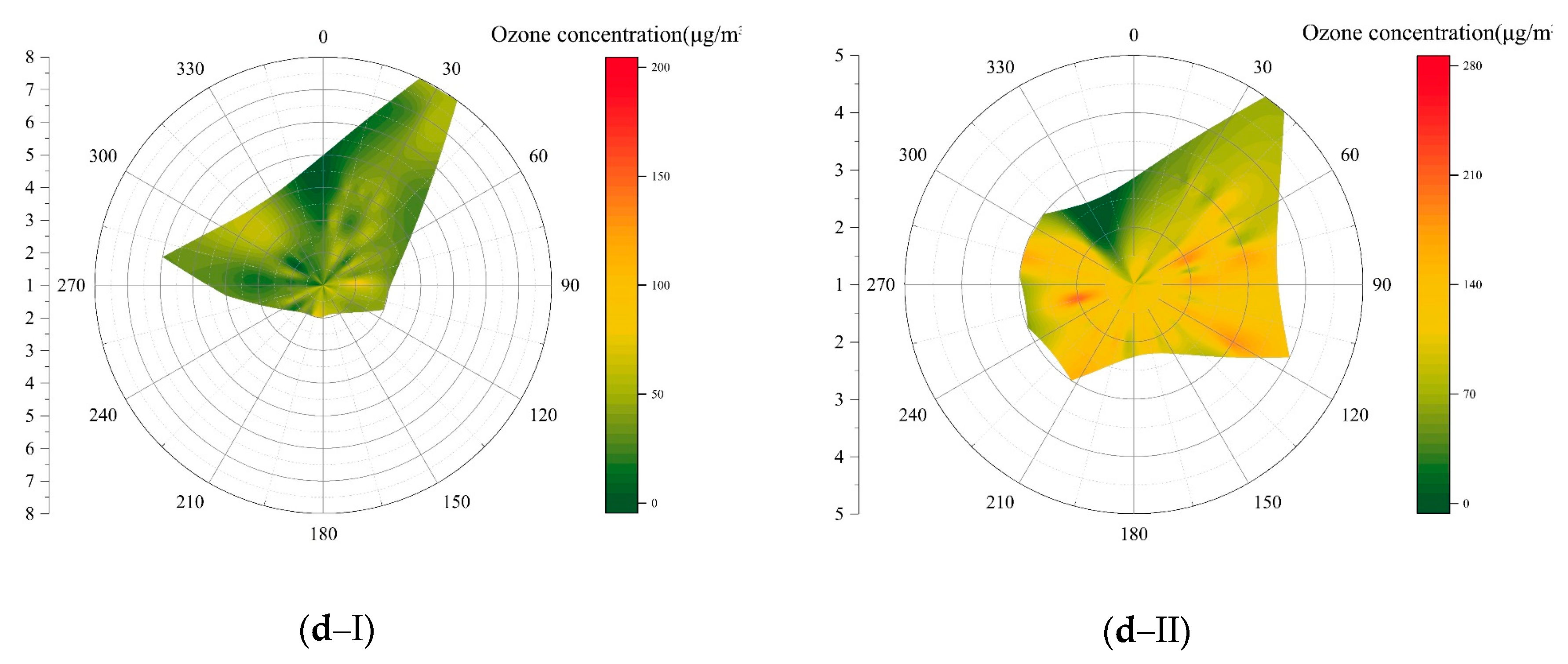
3.2.1. Spatial Distribution of Ozone Pollution in Shandong

By applying inverse distance weighting (IDW) to the MDA8 of each station, the spatial distributions of ozone pollution in Shandong from 2014–2018 were preliminarily analyzed (Figure 4). In general, the city with the most serious ozone pollution was Dongying (DY) and that with the least was WH; the results also roughly showed high concentrations of ozone in the plains and low concentrations along the Yellow Sea and the mountains. In 2014 and 2015, the high-value centers in the province appeared in DY and WF, and the difference between the cities was significant. In subsequent years, the high-value center gradually moved westward to JNA, BZ and ZZ, and the difference in pollution levels throughout Shandong province was reduced significantly.

3.2.2. EOF Analysis

The MDA8 ozone concentration in 2014–2018 was analyzed by EOF analysis, and the three modes with the largest contribution rate of variance (about 90%) were selected for key analysis (Figure 5).
The first EOF pattern (EOF1) explained 81.33% of the total variance in daily MDA8 ozone. In this pattern, the distribution of ozone was consistent throughout Shandong province. The high-value center is in the northwestern part of Shandong and the northern part of LZ, while the low-value center was in the Peninsula Coastal area, showing the distribution characteristics of high concentrations in inland areas and low concentrations in coastal areas. The time weight coefficient series corresponding to the pattern showed significant seasonal variation, and the high concentration value daytime with a positive coefficient was concentrated from May to September. The time weight coefficient was less than zero in winter, indicating low time ozone concentrations (Figure S3). This pattern is mainly caused by solar radiation, seasonal changes in temperature, and differences in VOCs and NOx emissions caused by industrial structures in different regions of Shandong.
The second EOF pattern (EOF2) explained 5.46% of the total variance in daily MDA8 ozone, showing the spatial difference in ozone distribution in Shandong. Almost exactly the opposite of the EOF1, the high-value center was in the Peninsula Coastal area in EDF2, while the low-value center appeared in the northwestern part of Shandong and the northern part of LZ. The seasonal variations of the time weight coefficient series are not obvious, and positive or negative values appeared throughout the whole year; however, the summer was slightly higher than other seasons (Figure S3). The main influencing factor of this pattern is the local circulation, and the coastal areas show different ozone distribution patterns from the inland areas under the influence of the obvious local circulation. Sea–land breeze can occur all year round but is the strongest in summer, hence the time weight coefficient was slightly higher in summer. In addition, compared with inland cities, the concentration of particulate matter in the coastal areas was lower and the atmospheric transparency was higher, which resulted in the final ozone distribution pattern.
The third EOF pattern (EOF3) explained 3.09% of the total variance in daily MDA8 ozone and showed the spatial difference of ozone distribution in Shandong. In this pattern, the high-value center appears in the LN, while the low-value center appeared in the northwestern part of Shandong and the northern part of the peninsula area, showing a decreasing trend with the increasing latitude. Similar to the EOF2, the seasonal variation of the time weight coefficient series is not obvious, but is slightly higher in summer than in other seasons (Figure S3). The main influencing factor was the regional-scale ozone transport. During summer, pollutants from southern provinces can be transported to Shandong by the prevailing southerly wind. This cross-regional transport has a significant impact on the LN, and with the increased of transmission distance, especially with the barrier of the mountains in LZ, the pollutants from the south have less impact on the northwestern part of Shandong and the northern part of the PA.
It was interesting that when the time weight coefficient of the EOF3 was large, the time weight coefficient of EOF2 tended to be lower (Figure S3) because large-scale circulation suppresses local circulation [54]. The higher variance contribution rate of EOF2 reflects that the impact of small-scale meteorological systems on the distribution of ozone in Shandong province is greater than that of large-scale systems.
Compared with other regions, the main pattern of Jiangsu province in China explains 73% of the total variance in daily MDA8 ozone, and the time weight coefficient is reduced with increasing latitude [55]. It is considered to be caused by solar radiation, seasonal changes in temperature and differences in VOCs emissions caused by different industries. The main pattern in the eastern United States only explains 73% of the total variance in daily MDA8 ozone, showing a low eigenvalue distribution in the northeast and the Midwest, which is believed to reflect the effects of polar jets from the Great Lakes [38]. India’s primary pattern explains 60% of the total variance in daily MDA8 ozone, showing the high distribution in the northwest and low distribution in the south and marine areas, which is believed to reflect the effects of the monsoon [47]. In this view, the main cause of the distribution pattern of ozone concentration in Shandong was similar to that in Jiangsu.

3.2.3. Cluster Analysis

Based on the MDA8, cluster analysis was used to classify the monitoring sites to further understand the characteristics of ozone pollution in different regions of Shandong province (Figure 6). The central stations were selected from the high load area in EOF1. Cities with similar trends in MDA8 were clustered into one cluster that represented the regional air pollution characteristics affected by large-scale circulation or regional transportation [56].
Cluster I: Peninsula Coastal area (PC), including RZ, QD, YT, and WH, located in the eastern Shandong province. The annual classification of cluster I was very stable. Maritime characteristics were obvious in this cluster and ozone concentrations showed a low peak value and a high valley value. In this cluster, the daily and annual differences in ozone concentrations were unnoticeable; however, the average hourly ozone concentration was the highest in Shandong. This feature was more prominent in the area affected more by the ocean, such as the typical representative city of Weihai.
Cluster II: Lunan inland area (LN), including HZ, JNI, LY, and ZZ, located in the south of Mount Tai. The annual classification of this cluster was also relatively stable, and the level of ozone pollution was in the middle reaches of Shandong. This cluster has a large load in the EOF3 area, indicating that it is greatly influenced by the cross-region transport of ozone from the south of the province.
Cluster III: Western Bohai area (WB), including DY, WF, and BZ, located in the eastern areas of the northern Mount Tai. The annual division of this cluster is relatively stable, and in certain years (2014, 2015) its characteristics were close to those of cluster IV. According to the 90th percentile of the MDA8, this area had the highest level of ozone pollution. Although it is coastal, the maritime nature was not obvious due to the concentrated population and industrial activity in the inland areas. Its valley value was low and peak value was the highest, which may be related to the presence of enterprises such as the petroleum and chemical industries, which emit high levels of VOCs.
Cluster IV: Luxi plain area (LX), including DZ, LC, northern JNA, northern ZB, and northern TA, located in the western areas of northern Mount Tai. The annual division of this cluster was not stable, especially for the southern part, which is a transition zone between plains and mountains. The pollution was complicated and varied with the changes of the pressure field and wind direction. The ozone pollution of this area was serious, which was related to high emissions of precursors from the concentrated population and industries.
Cluster V: Luzhong mountain area (LZ), including LW, southern JNA, southern ZB, southern TA, located in Mount Tai. The annual classification of cluster V is unstable. Ozone pollution was relatively low in these clusters. There is a lower population and fewer industrial activities in the mountains, and production activities here are mainly related to low VOCs and NOx emissions such as those from agriculture.
The spatial distribution characteristics of ozone in Shandong province were accordant with other regions with similar topography, such as China’s Sichuan Basin and California’s San Joaquin Valley, where five and six clusters were obtained respectively [56,57]. As for Jiangsu, which was dominated by plains and the population was concentrated in the inland areas, only three clusters were obtained [55]. These results confirmed that complex terrain, such as mountains and seas, made the distribution of ozone pollution more complex. Terrain affects the formation and transmission of ozone by affecting the development of mesoscale weather systems [58], and leads to the population and economic activities concentrating in areas with suitable geographical conditions; this resulted in the uneven distribution of precursors in these areas.

4. Discussion

4.1. Meteorological Factors

4.1.1. Solar Radiation

The correlation between the monthly ozone concentration and monthly local total solar radiation was calculated to explore the influence of solar radiation. Since solar radiation occurs only during the daytime, the monthly ozone concentration was the average of the MDA8.
The results showed significant correlation between solar radiation and local ozone concentration (p < 0.05) (Table S1) and the correlation coefficient increased year by year. The solar radiation-ozone concentration scatter plots in summer (May–September; Figure S4) showed that ozone pollution has deteriorated year by year, even when solar radiation conditions have been stable. The increase in emissions of ozone precursors made a large contribution to the elevated ozone concentrations.
Other studies have also shown that the ozone concentration is significantly positively correlated with solar radiation intensity [59,60]; however, most studies have discussed the daily or seasonal variations of ozone concentration, and fewer studies have focused on the relationship between interannual ozone concentration and solar radiation.

4.1.2. Air Temperature

Air temperature is another important meteorological factor affecting ground-level ozone concentrations [61], which increase approximately linearly over a temperature range of 17 °C to 32 °C [62]. Temperature can directly affect the ozone concentration by controlling the chemical reaction processes in the atmosphere [63], and can also affect the ozone dry deposition process by adjusting the absorption intensity of stomata [64]. As shown in Section 3.1, the daytime ozone concentration in coastal cities (QD, YT, WH, RZ) were lower than other inland cities, and this phenomenon can be explained by temperature differences.
Figure 7 shows the temperature distribution of two typical coastal cities (WH, YT) and two typical inland cities (JNA, located north of Mount Tai; LY, located south of Mount Tai) in 2018. Air temperatures in the two inland cities during the day were significantly higher than in the two coastal cities, especially in the afternoon. Differences of ozone concentrations in coastal and inland areas caused by temperature have also been observed in Sweden, Spain and Poland [65,66,67].

4.1.3. Local Circulation

The nighttime ozone concentrations in coastal cities (QD, YT, WH and RZ) were significantly higher than those in inland cities (Figure 3), this was related to the local circulation of coastal cities. Figure 8 shows the wind directions, wind frequency and ozone concentrations at 2 am and 2 pm in two coastal (WH, YT) and inland (JNA, LY) cities in 2018. As shown in Figure 8, the prevailing wind direction in WH and YT during the day and night changed significantly. The prevailing winds were southwest from the land at night and northeast from the sea during the day in the coastal cities, whereas there was no obvious variation in the prevailing winds during the daytime and nighttime for the two inland cities.
To the east and north of the built-up area of WH and YT is the Yellow Sea and there are mountains southwest of the two cities. The mountains increase the intensity of the local wind [64]. The downhill wind and land breeze, and the uphill wind and sea breeze are superimposed, resulting in a stronger and a longer-lasting breeze [68]. During the daytime, the sea breeze from the northeast superimposes with the uphill wind, which removed the pollutants from the city and brought pollutants to the mountainous areas. Therefore, the ozone concentrations in the coastal cities decreased. At night, downhill winds superimpose with the land breeze, so that pollutants are transported back to the built-up area, resulting in high ozone concentrations in coastal cities at night. Similar results were obtained in Italy and Portugal [54,69], confirming the impact of local circulation on the spatial distribution of ozone. Due to the overall low altitude in the mountainous areas of Shandong (the highest altitude of Mount Tai is 1545 m) [70], the wind direction in the inland cities had no obvious variation.
In addition, the properties of the underlying surface are also responsible for the differences in the distribution of coastal and inland ozone concentrations. Brian K. Blaylock et al. considered that the deposition rate of ozone on the water is lower than that on the land, so that pollutants accumulate in coastal cities at night [71]. Håkan Pleijel et al. suggested that the land surface can form a stable boundary layer by radiative cooling at night, which can strongly restrict the vertical mixing of air and result in lower ozone concentrations in inland cities [72].

4.2. Anthropogenic Factors

The industry data of Shandong province were correlated with the annual average ozone concentration. The car ownership index (COI) based on average annual cars of per unit of built-up area can reflect the impact of motor vehicle emissions. The industries that emit precursors (VOCs and NOx) are correlated with ozone concentrations and the level of industrial activity is represented by the annual industrial output. Due to the lack of statistics on VOC emissions, only the annual NOx emissions data are used to correlate with ozone concentrations.
Correlation analysis showed that the COI, petroleum processing, and chemical industries were significantly positively correlated with ozone concentration. Other manufacturing industries including chemical fiber, rubber, and plastic products were not significantly correlated with ozone concentrations, while the NOx emissions were significantly negatively correlated with ozone concentration (Table 2). Among them, the petroleum processing industries and chemical industries are important sources of VOCs emissions [73], including boiler exhaust, leakage, evaporation, etc. [74]. Although automobile exhaust emits NOx and VOCs simultaneously, the positive correlation effect of vehicle exhaust may be mainly reflected in the emissions of VOCs, because of the positive correlation between the ozone concentration and NOx.
Suggested by the correlation analysis, the abatement of VOCs sources was necessary to better control ozone pollution in Shandong province, which was consistent with the studies carried out in central and eastern China [4,21,75]. The results suggested that the effect may be remarkable to control ozone pollution from automobile exhaust, petroleum processing, and chemical industries.

5. Conclusions

We studied the ground-level ozone concentrations in Shandong province from 2014 to 2018. The annual average ozone concentration increased year by year in Shandong. Due to the frequent high temperature, and the lower humidity and cloud cover, the annual peak ozone concentrations appeared in May or June, prior to the monsoon rainy season. In September, after the monsoon impact, certain coastal cities (e.g., Weihai) showed the second highest peak. The daily ozone concentration in all cities were unimodal; however, the daily ozone variation in coastal cities was significantly smaller than that in inland cities. In terms of spatial characteristics, the EOF analysis listed three main patterns of ozone concentration distribution in Shandong. The first pattern with the largest variance contribution rate reflects the influence of solar radiation, temperature, and industries. The other two patterns show the effects of sea–land differences and cross-regional transport from the south. Using the cluster analysis method, the ozone pollution in Shandong was divided into five clusters: Peninsula Coastal area (PC), Lunan inland area (LN), Western Bohai area (WB), Luxi plain area (LX), and Luzhong mountain area (LZ).
Meteorological and anthropogenic factors had significant influence on ground-level ozone concentrations. A significant positive correlation between ozone concentrations and solar radiation was observed, and even under similar conditions of solar radiation conditions, ozone pollution is deteriorating year by year. Affected by the temperature and local circulation between typical coastal cities (WH and YT) and inland cities (JNA and LY), the ozone concentrations in coastal cities were lower during the day and higher at night than in inland cities. The correlation analysis suggested that the average car ownership, petroleum processing, and chemical industries were significantly positively correlated with the ozone concentration, and that NOx emissions were significantly negatively correlated with the ozone concentration. Therefore, controlling pollution emissions from automobiles, petroleum processing, and chemical industries is recommended to mitigate the increasing ozone pollution in Shandong province. With the EOF and cluster analysis methods, this study analyzed the spatial and temporal characteristics of ozone distribution in Shandong province in 2014–2018, filling the research gap of ozone pollution in Shandong province in eastern China. Moreover, this study made meaningful explorations of the impacts of industrial structure and traffic on ozone pollution, and provided a possible way to control ozone pollution in Shandong province.

Supplementary Materials

The following are available online at https://www.mdpi.com/2073-4433/10/9/501/s1, Figure S1. Ozone concentrations in 17 Prefectural level cities of Shandong in 2014–2018 based on different methods (a, ozone hourly average concentration; b, annual average of MDA8; c, the 90th percentile of MDA8); Figure S2. Statistics of days exceeding ozone standard in 17 Prefectural level cities of Shandong in 2014–2018. The standard is the secondary standard of Ambient air quality standards GB 3095-2012 (160 μg/m3 for daily MDA8) (a), and the WHO standard, which is the primary standard of Ambient air quality standards GB 3095-2012 (100μg/m3 for daily MDA8) (b); Figure S3. The time weight coefficients of the main modes from the empirical orthogonal function analysis; Figure S4. Scatter plot of solar radiation and ozone monthly concentration in summer (May–September) of Shandong province, Table S1 Solar radiation and ozone concentration correlation analysis results.

Author Contributions

Conceptualization, J.Z., H.L. and M.W.; Data curation, K.Q., J.D. and H.L.; Formal analysis, J.Z., J.D. and Y.S.; Funding acquisition, M.W.; Investigation, K.Q.; Methodology, J.Z. and C.W.; Project administration, M.W.; Resources, K.Q. and H.L.; Software, J.Z. and C.W.; Supervision, M.W.; Visualization, J.Z., J.D. and Y.S.; Writing—original draft, J.Z.; Writing—review and editing, H.L. and M.W.

Funding

This research was funded by the National Natural Science Foundation of China (41605113), China Postdoctoral Science Foundation (2019T120606, 2018M632713).

Acknowledgments

We thank the Shandong Province Environment Information and Monitoring Center to provide the air quality data.

Conflicts of Interest

The authors declare no conflict of interest.

References

  1. Wang, Y.; Du, H.; Xu, Y.; Lu, D.; Wang, X.; Guo, Z. Temporal and spatial variation relationship and influence factors on surface urban heat island and ozone pollution in the Yangtze River Delta, China. Sci. Total Environ. 2018, 631–632, 921–933. [Google Scholar] [CrossRef] [PubMed]
  2. Gao, W.; Tie, X.; Xu, J.; Huang, R.; Mao, X.; Zhou, G.; Chang, L. Long-term trend of O-3 in a mega city (Shanghai), China: Characteristics, causes, and interactions with precursors. Sci. Total Environ. 2017, 603, 425–433. [Google Scholar] [CrossRef] [PubMed]
  3. Teresa Pay, M.; Gangoiti, G.; Guevara, M.; Napelenok, S.; Querol, X.; Jorba, O.; Perez Garcia-Pando, C. Ozone source apportionment during peak summer events over southwestern Europe. Atmos. Chem. Phys. 2019, 19, 5467–5494. [Google Scholar] [Green Version]
  4. Wang, T.; Xue, L.; Brimblecombe, P.; Lam, Y.F.; Li, L.; Zhang, L. Ozone pollution in China: A review of concentrations, meteorological influences, chemical precursors, and effects. Sci. Total Environ. 2017, 575, 1582–1596. [Google Scholar] [CrossRef] [PubMed]
  5. Feng, Z.; Hu, E.; Wang, X.; Jiang, L.; Liu, X. Ground-level O3 pollution and its impacts on food crops in China: A review. Environ. Pollut. 2015, 199, 42–48. [Google Scholar] [CrossRef]
  6. Goodman, J.E.; Prueitt, R.L.; Sax, S.N.; Pizzurro, D.M.; Ynch, E.N.L.; Zu, K.; Venditti, F.J. Ozone exposure and systemic biomarkers: Evaluation of evidence for adverse cardiovascular health impacts. Crit. Rev. Toxicol. 2015, 45, 412–452. [Google Scholar] [CrossRef] [PubMed]
  7. Cakmak, S.; Hebbern, C.; Vanos, J.; Crouse, D.L.; Burnett, R. Ozone exposure and cardiovascular-related mortality in the Canadian Census Health and Environment Cohort (CANCHEC) by spatial synoptic classification zone. Environ. Pollut. 2016, 214, 589–599. [Google Scholar] [CrossRef] [Green Version]
  8. Zhang, Y.; Cooper, O.R.; Gaudel, A.; Thompson, A.M.; Nedelec, P.; Ogino, S.-Y.; West, J.J. Tropospheric ozone change from 1980 to 2010 dominated by equatorward redistribution of emissions. Nat. Geosci. 2016, 9, 875–879. [Google Scholar] [CrossRef]
  9. Lu, H.; Lyu, X.; Cheng, H.; Ling, Z.; Guo, H. Overview on the spatial-temporal characteristics of the ozone formation regime in China. Environ. Sci. Proc. Impacts 2019, 21, 916–929. [Google Scholar] [CrossRef]
  10. Peng, R.D.; Bell, M.L.; Geyh, A.S.; McDermott, A.; Zeger, S.L.; Samet, J.M.; Dominici, F. Emergency admissions for cardiovascular and respiratory diseases and the chemical composition of fine particle air pollution. Environ. Health Persp. 2009, 117, 957–963. [Google Scholar] [CrossRef]
  11. Gao, Y.; Zhang, M. Sensitivity analysis of surface ozone to emission controls in Beijing and its neighboring area during the 2008 Olympic Games. J. Environ. Sci. 2012, 24, 50–61. [Google Scholar] [CrossRef]
  12. Lin, X.; Yuan, Z.; Yang, L.; Luo, H.; Li, W. Impact of extreme meteorological events on ozone in the Pearl River Delta, China. Aerosol Air Qual. Res. 2019, 19, 1307–1324. [Google Scholar] [CrossRef]
  13. Xu, Z.; Huang, X.; Nie, W.; Chi, X.; Xu, Z.; Zheng, L.; Sun, P.; Ding, A. Influence of synoptic condition and holiday effects on VOCs and ozone production in the Yangtze River Delta region, China. Atmos. Environ. 2017, 168, 112–124. [Google Scholar] [CrossRef]
  14. Mbululo, Y.; Qin, J.; Hong, J.; Yuan, Z. Characteristics of atmospheric boundary layer structure during PM2.5 and ozone pollution events in Wuhan, China. Atmosphere 2018, 9, 359. [Google Scholar] [CrossRef]
  15. Tan, Z.; Lu, K.; Jiang, M.; Su, R.; Dong, H.; Zeng, L.; Xie, S.; Tan, Q.; Zhang, Y. Exploring ozone pollution in Chengdu, southwestern China: A case study from radical chemistry to O-3-VOC-NOx sensitivity. Sci. Total Environ. 2018, 636, 775–786. [Google Scholar] [CrossRef] [PubMed]
  16. Qin, L.; Gu, J.; Liang, S.; Fang, F.; Bai, W.; Liu, X.; Zhao, T.; Walline, J.; Zhang, S.; Cui, Y.; et al. Seasonal association between ambient ozone and mortality in Zhengzhou, China. Int. J. Biometeorol. 2017, 61, 1003–1010. [Google Scholar] [CrossRef] [PubMed]
  17. Yao, Y.; He, C.; Li, S.; Ma, W.; Li, S.; Yu, Q.; Mi, N.; Yu, J.; Wang, W.; Yin, L.; et al. Properties of particulate matter and gaseous pollutants in Shandong, China: Daily fluctuation, influencing factors, and spatiotemporal distribution. Sci. Total Environ. 2019, 660, 384–394. [Google Scholar] [CrossRef] [PubMed]
  18. Yang, Y.; Christakos, G. Spatiotemporal characterization of ambient PM2.5 concentrations in Shandong Province (China). Environ. Sci. Technol. 2015, 49, 13431–13438. [Google Scholar] [CrossRef]
  19. Xue, R.; Ai, B.; Lin, Y.; Pang, B.; Shang, H. Spatial and temporal distribution of aerosol optical depth and its relationship with urbanization in Shandong Province. Atmosphere 2019, 10, 110. [Google Scholar] [CrossRef]
  20. Shan, W.; Yin, Y.; Zhang, J.; Ji, X.; Deng, X. Surface ozone and meteorological condition in a single year at an urban site in central-eastern China. Environ. Monit. Assess. 2009, 151, 127–141. [Google Scholar] [CrossRef]
  21. Sun, L.; Xue, L.; Wang, T.; Gao, J.; Ding, A.; Cooper, O.R.; Lin, M.; Xu, P.; Wang, Z.; Wang, X.; et al. Significant increase of summertime ozone at Mount Tai in Central Eastern China. Atmos. Chem. Phys. 2016, 16, 10637–10650. [Google Scholar] [CrossRef] [Green Version]
  22. Yang, F.; Wang, T.; Shu, L.; Zhao, M.; Chen, P.; Li, M.; Yang, D.; Wang, J.; Xu, S. Characteristics and mechanisms for a heavy O3 pollution episode in Qingdao coastal area. Acta Scien. Circum. 2019, 1–14. [Google Scholar]
  23. Krishna, P.V.; Toshimasa, O.C.; Chris, J. Land-Atmospheric Research Applications in South and Southeast Asia, 1st ed.; Springer International Publishing: Cham, Switzerland, 2018; pp. 255–275. [Google Scholar]
  24. Otero, N.; Sillmann, J.; Schnell, J.L.; Rust, H.W.; Butler, T. Synoptic and meteorological drivers of extreme ozone concentrations over Europe. Environ. Res. Lett. 2016, 11, 024005. [Google Scholar] [CrossRef]
  25. Dawson, J.P.; Adams, P.J.; Pandis, S.N. Sensitivity of ozone to summertime climate in the eastern USA: A modeling case study. Atmos. Environ. 2007, 41, 1494–1511. [Google Scholar] [CrossRef]
  26. Tao, Z.; Williams, A.; Huang, H.C.; Caughey, M.; Liang, X.Z. Sensitivity of U.S. surface ozone to future emissions and climate changes. Geophys. Res. Lett. 2007, 34, 402–420. [Google Scholar] [CrossRef]
  27. Coates, J.; Mar, K.A.; Ojha, N.; Butler, T.M. The influence of temperature on ozone production under varying NOx conditions—A modelling study. Atmos. Chem. Phys. 2016, 16, 11601–11615. [Google Scholar] [CrossRef]
  28. Zhao, S.; Yu, Y.; Yin, D.; He, J.; Liu, N.; Qu, J.; Xiao, J. Annual and diurnal variations of gaseous and particulate pollutants in 31 provincial capital cities based on in situ air quality monitoring data from China National Environmental Monitoring Center. Environ. Int. 2016, 86, 92–106. [Google Scholar] [CrossRef]
  29. Bei, N.; Zhao, L.; Wu, J.; Li, X.; Feng, T.; Li, G. Impacts of sea-land and mountain-valley circulations on the air pollution in Beijing-Tianjin-Hebei (BTH): A case study. Environ. Pollut. 2018, 234, 429–438. [Google Scholar] [CrossRef]
  30. Liu, Z.J.; Xie, X.X.; Xie, M.; Wang, T.J.; Shu, L. Spatio-temporal distribution of ozone pollution over Yangtze River Delta region. J. Ecol. Rural Environ. China 2016, 32, 445–450. [Google Scholar]
  31. Zhang, Y.N.; Xiang, Y.R.; Chan, L.Y.; Chan, C.Y.; Sang, X.F.; Wang, R.; Fu, H.X. Procuring the regional urbanization and industrialization effect on ozone pollution in Pearl River Delta of Guangdong, China. Atmos. Environ. 2011, 45, 4898–4906. [Google Scholar] [CrossRef]
  32. Xiao, K.; Wang, Y.; Wu, G.; Fu, B.; Zhu, Y. Spatiotemporal characteristics of air pollutants (PM10, PM2.5, SO2, NO2, O3, and CO) in the inland basin city of Chengdu, southwest China. Atmosphere 2018, 9, 74. [Google Scholar] [CrossRef]
  33. Li, G.; Bei, N.; Cao, J.; Wu, J.; Long, X.; Feng, T.; Dai, W.; Liu, S.; Zhang, Q.; Tie, X. Widespread and persistent ozone pollution in eastern China during the non-winter season of 2015: observations and source attributions. Atmos. Chem. Phys. 2017, 17, 2759–2774. [Google Scholar] [CrossRef] [Green Version]
  34. Niu, H.; Mo, Z.; Shao, M.; Lu, S.; Xie, S. Screening the emission sources of volatile organic compounds (VOCs) in China by multi-effects evaluation. Front. Env. Sci. Eng. 2016, 10, 1. [Google Scholar] [CrossRef]
  35. Shi, Y.; Xia, Y.-f.; Lu, B.-h.; Liu, N.; Zhang, L.; Li, S.-j.; Li, W. Emission inventory and trends of NOx for China, 2000–2020. J. Zhejiang. Uuiv. Sci. A 2014, 15, 454–464. [Google Scholar] [CrossRef]
  36. Ding, Y.G.; Zhang, Y.C. A new cluster method for climatic classification and compartment using the conjunction between CAST and REOF. Chin. J. Atmos. Sci. 2007, 31, 129–136. [Google Scholar]
  37. Weare, B.C.; Nasstrom, J.S. Examples of extended empirical orthogonal function analyses. Mon. Weather Rev. 1982, 110, 481. [Google Scholar] [CrossRef]
  38. Shen, L.; Mickley, L.J.; Tai, A.P.K. Influence of synoptic patterns on surface ozone variability over the eastern United States from 1980 to 2012. Atmos. Chem. Phys. 2015, 15, 10925–10938. [Google Scholar] [CrossRef] [Green Version]
  39. Zhao, Z.; Wang, Y. Influence of the West Pacific subtropical high on surface ozone daily variability in summertime over eastern China. Atmos. Environ. 2017, 170, 197–204. [Google Scholar] [CrossRef]
  40. Pavon-Dominguez, P.; Jimenez-Hornero, F.J.; Gutierrez de Rave, E. Proposal for estimating ground-level ozone concentrations at urban areas based on multivariate statistical methods. Atmos. Environ. 2014, 90, 59–70. [Google Scholar] [CrossRef]
  41. Xiao-gang, H.; Jing-bo, Z.; Jun-ji, C.; Yong-yong, S. Spatial-temporal variation of ozone concentration and its driving factors in China. Environ. Sci. China 2019, 40, 1120–1131. [Google Scholar]
  42. Zhao, H.; Zheng, Y.; Li, T.; Wei, L.; Guan, Q. Temporal and spatial variation in, and population exposure to, summertime ground-level ozone in Beijing. Int. J. Environ. Res. Public Health 2018, 15, 628. [Google Scholar] [CrossRef]
  43. Wang, Z.Y.; Ding, Y.H. Climatic characteristics of rainy seasons in China. Chin. J. Atmos. Sci. 2008, 32, 1–13. [Google Scholar]
  44. Wang, Z.S.; Yun-Ting, L.I.; Chen, T.; Zhang, D.W.; Sun, F.; Sun, R.W.; Dong, X.; Sun, N.D.; Pan, L.B. Temporal and spatial distribution characteristics of ozone in Beijing. Environ. Sci. China 2014, 35, 4446. [Google Scholar]
  45. Wang, H.; Lijun, Z.; Xiaoyan, T. Ozone concentrations in rural regions of the Yangtze Delta in China. J. Atmos. Chem. 2006, 54, 255–265. [Google Scholar]
  46. Wang, Y.; Yu, C.; Tao, J.; Wang, Z.; Si, Y.; Cheng, L.; Wang, H.; Zhu, S.; Chen, L. Spatio-temporal characteristics of tropospheric ozone and its precursors in Guangxi, south China. Atmosphere 2018, 9, 355. [Google Scholar] [CrossRef]
  47. Hakim, Z.Q.; Archer-Nicholls, S.; Beig, G.; Folberth, G.A.; Sudo, K.; Abraham, N.L.; Ghude, S.; Henze, D.K.; Archibald, A.T. Evaluation of tropospheric ozone and ozone precursors in simulations from the HTAPII and CCMI model intercomparisons—A focus on the Indian subcontinent. Atmos. Chem. Phys. 2019, 19, 6437–6458. [Google Scholar] [CrossRef]
  48. Yusoff, M.F.; Latif, M.T.; Juneng, L.; Khan, M.F.; Ahamad, F.; Chung, J.X.; Mohtar, A.A.A. Spatio-temporal assessment of nocturnal surface ozone in Malaysia. Atmos. Environ. 2019, 207, 105–116. [Google Scholar] [CrossRef]
  49. Li, Q.; Gabay, M.; Rubin, Y.; Raveh-Rubin, S.; Rohatyn, S.; Tatarinov, F.; Rotenberg, E.; Ramati, E.; Dicken, U.; Preisler, Y.; et al. Investigation of ozone deposition to vegetation under warm and dry conditions near the Eastern Mediterranean coast. Sci. Total Environ. 2019, 658, 1316–1333. [Google Scholar] [CrossRef]
  50. Shu, L.; Xie, M.; Wang, T.; Gao, D.; Chen, P.; Han, Y.; Li, S.; Zhuang, B.; Li, M. Integrated studies of a regional ozone pollution synthetically affected by subtropical high and typhoon system in the Yangtze River Delta region, China. Atmos. Chem. Phys. 2016, 16, 15801–15819. [Google Scholar] [CrossRef] [Green Version]
  51. Lal, S.; Naja, M.; Subbaraya, B.H. Seasonal variations in surface ozone and its precursors over an urban site in India. Atmos. Environ. 2000, 34, 2713–2724. [Google Scholar] [CrossRef]
  52. Grigorieva, V.; Kolev, N.; Donev, E.; Ivanov, D.; Mendeva, B.; Evgenieva, T.; Danchovski, V.; Kolev, I. Surface and total ozone investigations in the region of Sofia, Bulgaria. Int. J. Remote Sens. 2012, 33, 3542–3556. [Google Scholar] [CrossRef]
  53. Andersson, C.; Langner, J.; Bergstrom, R. Interannual variation and trends in air pollution over Europe due to climate variability during 1958–2001 simulated with a regional CTM coupled to the ERA40 reanalysis. Tellus B 2007, 59, 77–98. [Google Scholar] [CrossRef]
  54. Federico, S.; Pasqualoni, L.; De Leo, L.; Bellecci, C. A study of the breeze circulation during summer and fall 2008 in Calabria, Italy. Atmos. Res. 2010, 97, 1–13. [Google Scholar] [CrossRef]
  55. Zhang, X.; Chen, W.; Huang, Y.; Qin, Y.; Qin, W.; Yang, X.; Weiqing, L.U. Temporal and spatial distribution characteristics of ozone in Jiangsu Province during 2013–2016. Environ. Monit. China 2017, 33, 50–58. [Google Scholar]
  56. Zhao, S.; Yu, Y.; Qin, D.; Yin, D.; Dong, L.; He, J. Analyses of regional pollution and transportation of PM2.5 and ozone in the city clusters of Sichuan Basin, China. Atmos. Pollut. Res. 2019, 10, 374–385. [Google Scholar] [CrossRef]
  57. Jin, L.; Harley, R.A.; Brown, N.J. Ozone pollution regimes modeled for a summer season in California’s San Joaquin Valley: A cluster analysis. Atmos. Environ. 2011, 45, 4707–4718. [Google Scholar] [CrossRef]
  58. Carvalho, A.C.; Carvalho, A.; Gelpi, I.; Barreiro, M.; Borrego, C.; Miranda, A.I.; Perez-Munuzuri, V. Influence of topography and land use on pollutants dispersion in the Atlantic coast of Iberian Peninsula. Atmos. Environ. 2006, 40, 3969–3982. [Google Scholar] [CrossRef]
  59. Wei, Z.; Bo, G.; Ming, L.; Qing, L.; She-xia, M.; Jia-ren, S.; Lai-guo, C.; Shao-jia, F. Impact of meteorological factors on the ozone pollution in Hong Kong. Environ. Sci. China 2019, 40, 55–66. [Google Scholar]
  60. Mohan, S.; Saranya, P. Assessment of tropospheric ozone at an industrial site of Chennai megacity. J. Air Waste Manag. 2019. [Google Scholar] [CrossRef]
  61. Duan, X.-T.; Cao, N.-W.; Wang, X.; Zhang, Y.-X.; Liang, J.-S.; Yang, S.-P.; Song, X.-Y. Characteristics analysis of the surface ozone concentration of China in 2015. Environ. Sci. China 2017, 38, 4976–4982. [Google Scholar]
  62. Steiner, A.L.; Davis, A.J.; Sillman, S.; Owen, R.C.; Michalak, A.M.; Fiore, A.M. Observed suppression of ozone formation at extremely high temperatures due to chemical and biophysical feedbacks. Proc. Natl. Acad. Sci. USA 2010, 107, 19685–19690. [Google Scholar] [CrossRef] [Green Version]
  63. Stathopoulou, E.; Mihalakakou, G.; Santamouris, M.; Bagiorgas, H.S. On the impact of temperature on tropospheric ozone concentration levels in urban environments. J. Earth Syst. Sci. 2008, 117, 227–236. [Google Scholar] [CrossRef]
  64. Solberg, S.; Hov, O.; Sovde, A.; Isaksen, I.S.A.; Coddeville, P.; De Backer, H.; Forster, C.; Orsolini, Y.; Uhse, K. European surface ozone in the extreme summer 2003. J. Geophys. Res. Atmos. 2008, 113, 1–16. [Google Scholar] [CrossRef]
  65. Piikki, K.; Klingberg, J.; Karlsson, G.P.; Karlsson, P.E.; Pleijel, H. Estimates of AOT ozone indices from time-integrated ozone data and hourly air temperature measurements in southwest Sweden. Environ. Pollut. 2009, 157, 3051–3058. [Google Scholar] [CrossRef]
  66. Santurtun, A.; Carlos Gonzalez-Hidalgo, J.; Sanchez-Lorenzo, A.; Teresa Zarrabeitia, M. Surface ozone concentration trends and its relationship with weather types in Spain (2001–2010). Atmos. Environ. 2015, 101, 10–22. [Google Scholar] [CrossRef]
  67. Struzewska, J.; Jefimow, M. A 15-Year Analysis of surface ozone pollution in the context of hot spells episodes over Poland. Acta Geophys. 2016, 64, 1875–1902. [Google Scholar] [CrossRef]
  68. Federico, S.; Dalu, G.A.; Casella, L.; Bellecci, C.; Colacino, M. Atmospheric convergence diabatically generated in the CBL over a mountainous peninsula. Nuovo Cimento C 2001, 24, 223–243. [Google Scholar]
  69. Sousa, S.I.V.; Alvim-Ferraz, M.C.M.; Martins, F.G. Identification and origin of nocturnal ozone maxima at urban and rural areas of Northern Portugal-Influence of horizontal transport. Atmos. Environ. 2011, 45, 942–956. [Google Scholar] [CrossRef]
  70. Gao, J.; Wang, T.; Ding, A.; Liu, C. Observational study of ozone and carbon monoxide at the summit of mount Tai (1534 m a.s.l.) in central-eastern China. Atmos. Environ. 2005, 39, 4779–4791. [Google Scholar] [CrossRef]
  71. Blaylock, B.K.; Horel, J.D.; Crosman, E.T. Impact of lake breezes on summer ozone concentrations in the Salt Lake Valley. J. Appl. Meteorol. Climatol. 2017, 56, 353–370. [Google Scholar] [CrossRef]
  72. Pleijel, H.; Klingberg, J.; Karlsson, G.P.; Engardt, M.; Karlsson, P.E. Surface ozone in the marine environment-Horizontal ozone concentration gradients in coastal areas. Water Air Soil Poll. 2013, 224, 1603. [Google Scholar] [CrossRef]
  73. Zhang, J.; Zhao, Y.; Zhao, Q.; Shen, G.; Liu, Q.; Li, C.; Zhou, D.; Wang, S. Characteristics and source apportionment of summertime volatile organic compounds in a fast developing city in the Yangtze River Delta, China. Atmosphere 2018, 9, 373. [Google Scholar] [CrossRef]
  74. Wei, W.; Lv, Z.; Yang, G.; Cheng, S.; Li, Y.; Wang, L. VOCs emission rate estimate for complicated industrial area source using an inverse-dispersion calculation method: A case study on a petroleum refinery in Northern China. Environ. Pollut. 2016, 218, 681–688. [Google Scholar] [CrossRef]
  75. Wu, R.; Xie, S. Spatial distribution of ozone formation in China derived from emissions of speciated volatile organic compounds. Environ. Sci. Technol. 2017, 51, 2574–2583. [Google Scholar] [CrossRef]
Figure 1. Study Area of Shandong province, including 17 Prefectural level cities until 2018. A total of 154 national and provincial environmental air quality monitoring stations are labeled in the figure. The bold black line indicates the boundary of Shandong province, and the gray line indicates the city boundary.
Atmosphere 10 00501 g001
Figure 2. Monthly ozone concentrations of Shandong province in 2014–2018 ((a) five years average concentration; (b) 2014 average concentration; (c) 2015 average concentration; (d) 2016 average concentration; (e) 2017 average concentration; (f) 2018 average concentration).
Atmosphere 10 00501 g002aAtmosphere 10 00501 g002bAtmosphere 10 00501 g002c
Figure 3. Diurnal variation of ozone concentrations in 17 Prefectural level cities of Shandong province in 2014–2018 ((a) five years average concentration; (b) 2014 average concentration; (c) 2015 average concentration; (d) 2016 average concentration; (e) 2017 average concentration; (f) 2018 average concentration).
Atmosphere 10 00501 g003aAtmosphere 10 00501 g003bAtmosphere 10 00501 g003c
Figure 4. Spatial distribution of ozone concentrations of Shandong province in 2014–2018 ((a) five years average concentration; (b) 2014 average concentration; (c) 2015 average concentration; (d) 2016 average concentration; (e) 2017 average concentration; (f) 2018 average concentration).
Atmosphere 10 00501 g004aAtmosphere 10 00501 g004bAtmosphere 10 00501 g004c
Figure 5. The spatial distribution of the main patterns of EOF (a, EOF1; b, EOF2; c, EOF3).
Atmosphere 10 00501 g005aAtmosphere 10 00501 g005b
Figure 6. Cluster analysis of ozone concentrations in 17 Prefectural level cities of Shandong province in 2014–2018. Five clusters were obtained including Peninsula Coastal area (PC), Lunan inland area (LN), Western Bohai area (WB), Luxi plain area (LX) and Luzhong mountain area (LZ) ((a) 2014; (b) 2015; (c) 2016; (d) 2017; (e) 2018).
Atmosphere 10 00501 g006aAtmosphere 10 00501 g006bAtmosphere 10 00501 g006c
Figure 7. Air temperature and ozone concentrations for typical coastal and inland cities of Shandong province in 2018 ((a) WH; (b) YT; (c) JNA; (d) LY).
Atmosphere 10 00501 g007aAtmosphere 10 00501 g007bAtmosphere 10 00501 g007c
Figure 8. Wind direction, frequency and ozone concentrations at 2 am and 2 pm for typical coastal and inland cities of Shandong province in 2018 ((a) WH; (b) YT; (c) JNA; (d) LY; I, 2 am; II, 2 pm).
Atmosphere 10 00501 g008aAtmosphere 10 00501 g008b
Table 1. Comparison of ground-level ozone concentration in several areas.
AreasIndexesYearOzone Concentration (μg/m3)Data Sources
Shandong provinceThe annual average hourly ozone concentration201464 This study
201565
201667
201774
201877
The annual average MDA8201497
201599
2016103
2017112
2018115
The 90th percentile of the MDA82014161
2015166
2016170
2017184
2018186
ChinaThe 90th percentile of the MDA82014140http://www.cnemc.cn/
2015134
2016138
2017149
2018151
The central and eastern regions of ChinaThe 90th percentile of the MDA82015151Reference [41]
2017172
The BTH regionThe 90th percentile of the MDA82014162http://www.cnemc.cn/
2015162
2016172
2017193
2018199
The YRDThe 90th percentile of the MDA82014154
2015163
2016159
2017170
2018167
The PRDThe 90th percentile of the MDA82014156
2015145
2016151
2017165
MDA8, The annual mean ozone concentration of the maximum daily 8 h average; BTH, Beijing–Tianjin–Hebei Area; YRD, Yangtze River Delta; PRD, Pearl River Delta.
Table 2. Analysis of correlation between human factors and ozone concentrations.
ProjectPearson Correlation CoefficientSignificance Test
Car ownership index (COI)0.2630.03 *
Petroleum processing0.310.013 *
Chemical industries0.3440.006 **
Chemical fiber0.080.552
Rubber and plastic products0.1730.174
Ordinary machinery0.050.698
Special equipment0.1170.359
Electrical machinery and equipment manufacturing−0.2390.059
Electricity, heat production, and supply−0.0790.538
NOX−0.5770.015 *
Correlation significant, ** p < 0.01, * p < 0.05.

