Temperature Changes in the Maloti-Drakensberg Region: An Analysis of Trends for the 1960–2016 Period

1
Faculty of Natural and Agricultural Sciences, QwaQwa Campus, University of the Free State, Private Bag X13, Phuthaditjhaba 9866, Free State, South Africa
2
Afromontane Research Unit (ARU), QwaQwa Campus, University of the Free State, Private Bag X13, Phuthaditjhaba 9866, Free State, South Africa
*
Author to whom correspondence should be addressed.
Atmosphere 2019, 10(8), 471; https://doi.org/10.3390/atmos10080471
Submission received: 26 June 2019
/
Revised: 31 July 2019
/
Accepted: 2 August 2019
/
Published: 16 August 2019
(This article belongs to the Section Meteorology)
Abstract
:Nature has been adversely affected by increasing industrialization, especially during the latter part of the last century, as a result of accelerating technological development, unplanned urbanization, incorrect agricultural policies and deforestation, which have contributed to the elevated concentration of the greenhouse gases (GHGs) in the environment. GHG accumulation has an adverse impact on meteorological and hydro-meteorological parameters, particularly temperature. Temperature plays a prominent and well-known role in evaporation, transpiration and changes in water demand, and thus significantly affects both water availability and food security. Therefore, a systematic understanding of temperature is important for fighting food insecurity and household poverty. Variations in temperature are often assessed and characterized through trend analysis. Hence, the objective of this paper is to determine long-term trends in mean monthly maximum and minimum air temperatures for the Maloti-Drakensberg region. The Mann–Kendall test, a non-parametric test, was applied on mean air temperature for the 1960–2016 period. A significant rising trend (p < 0.001) was detected with a yearly change in the long term annual mean maximum and mean minimum temperature by 0.03 °C/annum and 0.01 °C/annum, respectively. This knowledge has important implications for both the state of the environment and livelihoods in the region, since its use can be useful in planning and policymaking in water resource management, biodiversity conservation, agriculture, tourism and other sectors of the economy within the region.
1. Introduction
Recently, the warming of the climate system (i.e., the increase of mean temperature) has been concluded in many researches carried out at different regions of the world [1]. The rise in global temperature caused by natural, as well as anthropogenic drivers, is unequivocal [2].
Africa is among the most vulnerable regions projected to be affected by climate change and variability, due to its low adaptability to the projected climate change impacts [2]. As the Earth warms, climate and weather variability will increase. Global warming will have significant consequences on the rate of occurrence and severity of extreme weather events, which are projected to increase in the rest of this century; this will result in serious consequences for human and natural systems and is expected to have many adverse impacts on the environment [3].
Since the early 1980s, atmospheric temperature has increased significantly in the equatorial and southern parts of Eastern Africa, where the average seasonal temperatures have risen over the past 50 years. The higher temperatures and more frequent heat waves between 1961 and 2008 have been observed in countries bordering the western part of the Indian Ocean [4]. This is consistent with the conclusion of [5] who reported that the frequency of temperature extremes increased significantly during the period 1961–2000. Extreme rainfall events have become more frequent since the end of the 1950s and 1970s [6]. The warming of the climate system, the increase in climate variability and changes in frequency and severity of extreme events can result in significant effects on the spread and distribution of pests, weeds and crops, and livestock diseases [7].
A combination of drought followed by heavy rainfall has led to the spreading of diseases such as rift valley fever and blue tongue in East Africa and the African horse’s disease in South Africa [8]. However, while climate change-related problems may affect the whole world, the mountain regions are expected to be more vulnerable than other regions [9] due to the fact that mountain regions are extremely sensitive by nature. Kohler, Wehrli and Jurek [10] maintain that large mountain ranges could be considered as climatic barriers, whose boundaries could shift due to climate change, with dire consequences for ecosystems, especially through habitat changes, as well as through increased frequency of occurrence of natural hazards and disruption of economic activities and land uses. Mountain climates often exhibit spatially complex patterns [11]. This is most evident in their effect on vertical gradients of microclimates, species distribution, availability of natural resources such as water, soil and biological resources and land uses. The elevation distribution of these conditions is expected to change with climate change, making them even more complicated in the future. For instance, elevation gradients of species are expected to shift as a result of climate change [12]. Unfortunately, due to the inaccessible nature of mountains there is a dearth of research on mountains and how they might be affected by climate change. Yet, there is need for this information since mountains are a platform for various economical activities such as agriculture, mining and tourism, as well as infrastructure that might be vulnerable to climate change and climate variability [10]. One of the factors limiting research in mountain regions is the paucity of climate data. In mountain regions, most of the meteorological stations are located in valleys, leaving slopes and peaks underrepresented [13,14]. This situation is particularly evident in the Maloti-Drakensberg region, which is the focus of the current study.
2. The Study Area
The current study was undertaken in the Maloti-Drakensberg region (the region lies between 28.49° and 31.38° S and between 27.04° and 29.72° E) with an area of around 39,750 km2 (see Figure 1). The Maloti-Drakensberg region comprises mountain ranges that rise to the altitude of about 3473 m above sea level (masl) in the northeast and dip down to a height of 1213 masl in the south. The region is ecologically complex and is characterized by rare ecosystems and endemic species. It is also characterized by a diversity of land uses, including agriculture, tourism and mining. In this region, the agricultural growing season starts from October to December (OND). The region consists of the major catchments on which Lesotho and South Africa rely on for water supply, namely the Thukela River Basin, which drains eastwards into the India Ocean, and the Sequ-Orange River Basin, which drains westward into the Atlantic.
3. Data Sets and Methods
Gridded maximum and minimum monthly temperature time series data for the study area was downloaded from Climate Explorer (available from https://climexp.knmi.nl) for the period 1960–2016. The data were obtained from the Climate Research Unit Time-Series (CRU-TS) at a resolution of 0.5° × 0.5°, and included annual average maximum and minimum temperatures used in this paper, as shown in Figure 2 and Figure 3, respectively. The average annual temperature for a certain year was calculated by dividing the sum of the average temperatures value of all the annual months by twelve.
Suitability of the Mann–Kendall (MK) Trend Test for Long-Term Trends Detection in Hydro-Meteorological Data
Numerous studies have used the MK test assess trends in climate time series data. The application of the MK test for assessing time series of climate data does not require the data to be normally distributed [15]. An example of hydrological applications of the Mann–Kendall trend test is provided by [16,17] who used the MK test to detect the trends and variability of 18 hydrological variables. Other researchers used the test to detect the trend in hydroclimatic parameters, for instance: precipitation and drought [18]; pollutants, temperature and humidity [19]; and drought indices [20]. Another example where the MK test was applied is the research that was undertaken in northeast India by [21], which assessed trends in temperature data. Yunling and Yiping [22] used monthly air temperature and precipitation data series from 19 stations along the Lancang River (China) for the period 1960–2000 to assess climate change trends.
It is obvious that the MK test’s popularity has increased over the years. This popularity stems from a number of advantages that it offers, some of which were highlighted by [23], including the following. Firstly, the test does not require the assumption of normality of data. Secondly, it is based on the median rather than the mean. The median is less sensitive than the mean to outliers. Thirdly, no prior transformation of data is required when using the test.
Despite its advantages and popularity, the MK test has not yet been widely used in assessing trends in temperature. Yet temperature is a key variable that can influence other meteorological variables. Hence, [24] argued that temperature has an influence on almost all hydrologic variables. When temperature increases, relative humidity decreases (and vice versa). Temperature also regulates evapotranspiration, and accordingly chances of precipitation as well.
The following four steps were taken in performing trend analysis:
The first step involved the application of the Lowess regression analysis. The Lowess regression test was applied on the annual average maximum and minimum data series to identify patterns over time. Lowess regression is a nonparametric technique. It has advantages over parametric tests because it can reveal trends and cycles in data that might not be easy to model with parametric tests.
The application of the Mann–Kendall (MK) [4,25] trend test was the second step. The MK trend test was applied on monthly, seasonal and annual temperature data series. The MAKESENS software was used to perform the test. The MAKESENS software was developed by [26]. It can compute both the trend and magnitude of changes in temperature. MAKESENS has been coded to firstly, detect monotonic increasing or decreasing trends existence, and secondly to determine the change magnitude using Sen’s slope estimation method [27].
The Mann–Kendall test statistic equations are given below:
where xj and xk are the average annual values for years j and k, j > k, respectively, n is the number of years.
where sgn (xj − xk) is the sign function
The variance of S denoted by VAR(S) is computed as:
where q denotes number of tied groups and tp represents the data values length in the pth group. The Z values of S and VAR(S) are calculated as follows:
Z with positive values reveals increasing trends while negative Z values indicate decreasing trends. The third step involved the use of Sen’s slope estimator method.
Estimation of the trend magnitude (i.e., annual change) is calculated by using Sen’s method proposed by [28] and extended by [29].
The Sen’s method uses a linear model to estimate the slope of the trend as follows:
where F(t) defined as a continuous monotonic positive or negative increasing function of time, Q is the slope estimate and B is a constant.
Initially the slopes of all data value pairs are calculated as follows:
As the numbers of slopes Qi will be as many as N = n(n − 1)/2, n = number of time series years.
Then the median of these N values of Qi is the Sen’s estimator of slope as:
The final step required the application of the sequential t-test for analyzing regime shift (STARS) algorithm. The STARS algorithm was developed by [30] and is now widely used as a sequential model for change point detection in time series. Howard, Jarre, Clark and Moloney [31] stated that since the STARS algorithm relies on sequential analysis, this criterion differentiates it from the statistical empirical models used for point abruption detection. Based on the previously mentioned criterion, Rodionov and Overland [32] have shown that the STARS algorithm prevents weak performance towards the end of the time series. The STARS algorithm includes the regime shift index (RSI), which estimates the cumulative sum of normalized anomalies related to the critical level that has been determined by STARS (for more details see [30]).
The RSI equation is:
where, tcur represents the current time of the probation period, l is the cut-off length (e.g., number of years) of the regimes to be tested, xi is the value of the variable being tested, is the critical mean value of x, n is the number of years since the start of a new regime and Std denotes the average standard deviation for all one-year intervals in the time series. If the index becomes negative or positive at any time during the during the period under test from tcur to tcur + (l – 1) the index becomes negative or positive, the null hypothesis about the occurrence of a shift in the mean at time tcur is rejected, and the value xcur is included in the “current” regime. Otherwise, the time tcur is announced as a change point, c, referred to as a new regime [30].
4. Results and Discussion
For the period of 1960–2016, monthly, seasonal and average annual trends for maximum and minimum temperatures were analyzed using the MK test and Sen’s slope estimator method. The change point detection and RSI for maximum and minimum temperatures were defined by the STARS algorithm. Descriptive statistics of the annual average for maximum and minimum temperatures in the Maloti-Drakensberg region are summarized in Table 1 and Table 2, respectively. Variability of temperature in the region is indicated by the coefficient of variability (CoV) of 3.3% for maximum temperature and 5.1% for minimum temperature. The small value of CoV for the maximum and minimum temperatures indicates that the temperature in Maloti-Drakensberg has been relatively stable. Values of variance, skewness and kurtosis for the data were also estimated. Variance provides information about how far the variable value (maximum and minimum temperatures in this study) is located from its mean value. Results from the kurtosis test are shown in Table 1 and Table 2, which have negative values of −0.49 and −0.08 for maximum and minimum temperatures, respectively. Kurtosis is a measure that defines the shape of the probability function (e.g., oval or flat) compared to the normal distribution form. The lower negative value indicates that the variable probability function is slightly flatter than the normal distribution bell shape. The skew values were approximately 0.44 and 0.05, as shown in Table 1 and Table 2, respectively, which illustrate that the variable symmetrical distribution shape is located proportionally to the left and right of the mean value with a longer tail to the right for maximum temperature (higher value).
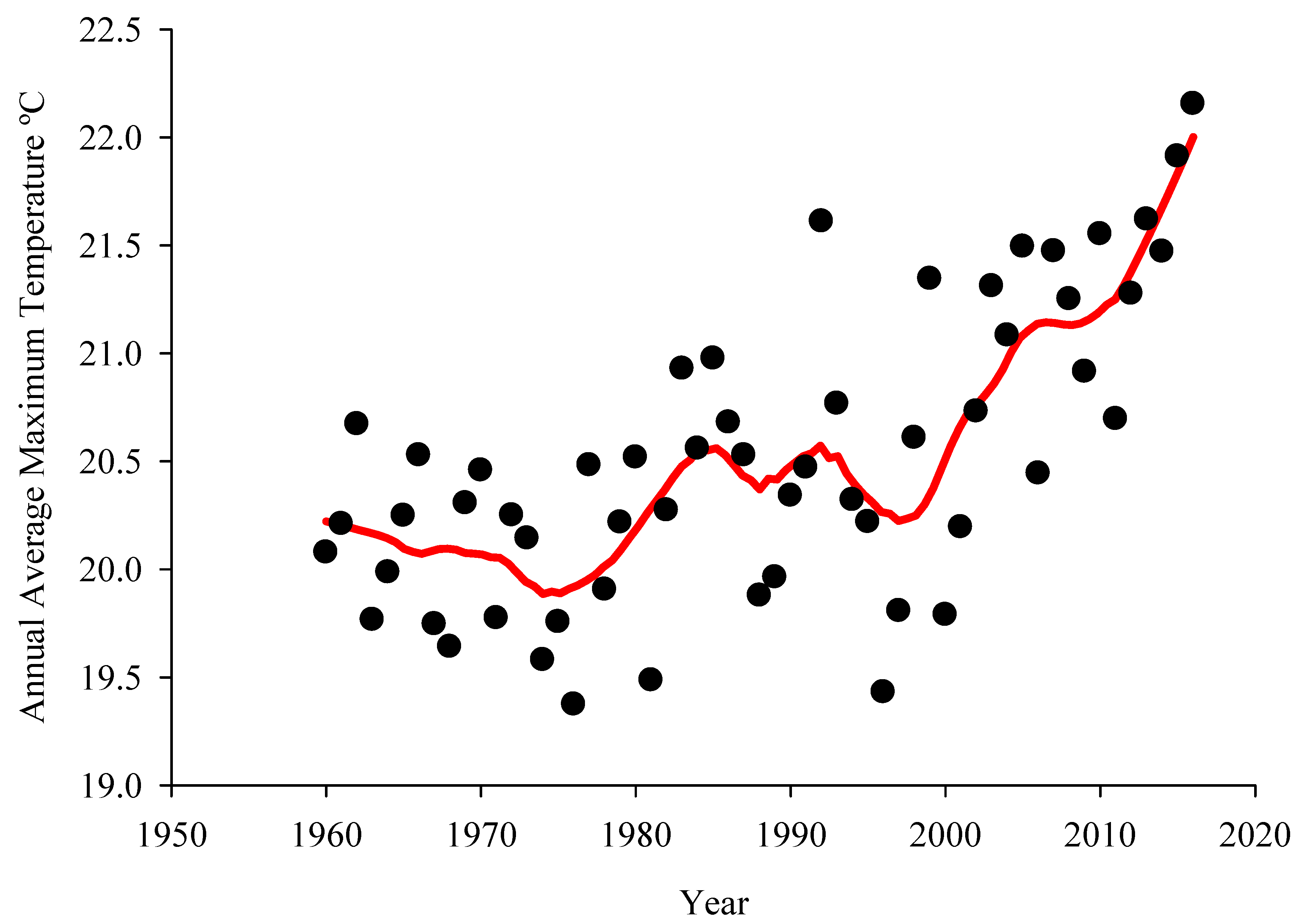
4.1. The Lowess Regression Curve
The Lowess regression curve [33] was applied to the annual average data series to picture the patterns over time. Figure 4 shows no significant trend for the first two decades in the maximum temperature, marginally increased after the first twenty years up to year 1985 followed by a decreasing trend thereafter up to year 1998. In the new millennium the trend has shown steep increasing up to the end of time series period span. Figure 5 shows the Lowess regression curves for the minimum temperature data series. Its curve depicts some similarity with the maximum temperature trend. Figure 5 shows a significant increasing trend from 1972 to 1986, after which the trend gradually decreased until 2011 when it started to increase again.
4.2. MK Test
4.3. Trend Analysis
Figure 6 and Figure 7 show the graphic variations of the trends for the annual average and OND maximum temperature while Figure 8 and Figure 9 depict the variability of annual average and OND minimum temperatures for the same period, respectively. As shown in Table 3, the results show a positive statistically significant trend for maximum temperature at all temporal scales. The exception is December, whose trend is not statistically significant. Similarly, the annual trend of maximum temperature is statistically significant (p = 0.001) at all time scales. The same applies for winter maximum temperatures, as shown in Table 3. This suggests that maximum temperatures have increased over the years. However, trends in minimum temperatures for the period between 1960 and 2016 are only statistically significant during the December, January and February months of the summer season and for May and June, during the winter season. This suggests that changes in minimum temperature have been mostly affected during the sub-seasons when temperature is either at its highest or lowest in the year. Nevertheless, annual trends of maximum temperature, just like minimum temperature, are statistically significant (p = 0.001). Sen’s slope of annual mean maximum and annual mean minimum temperature was 0.026 °C/annum and 0.009 °C/annum, respectively.
With regard to the start of the agricultural growing season, October–December (OND), results from the Sen’s slope analysis of temperature for the period of 1960–2016 are presented in Table 3 and Table 4, for maximum and minimum temperatures, respectively. A positive trend was noticed in the growing seasons for both maximum and minimum temperatures. The positive Sen’s slope indicates a rising trend in temperature, year-by-year (Figure 7 and Figure 9). The maximum seasonal temperature for OND was statistically significant at p = 0.01 (Sen’s slope = 0.019; as change per year). For minimum seasonal temperature for OND, the Sen’s slope results exhibited that the temperature had an increased trend (Sen’s slope = 0.008; as change per year, significant level greater than 1%). Significantly, the lesser calculated p-value of the temperature has statistical significance at 1%.
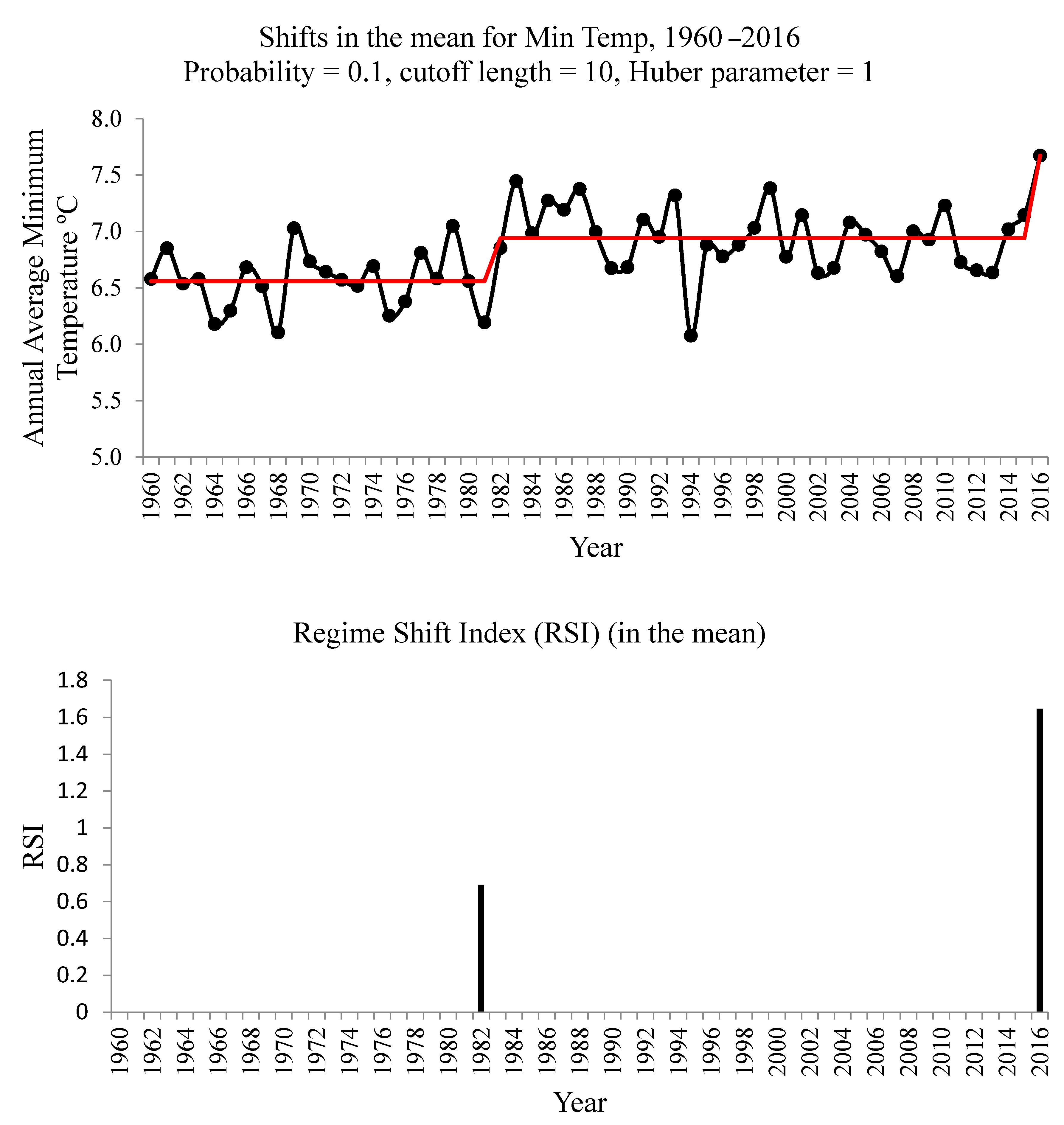
4.4. Change Point Detection
A regime shift index (RSI) component of the STARS algorithm [30] was used to assure the occurrence and statistical significance of abrupt changes in the temperature data sets. The RSI value is unitless which highlights the magnitude of the shift(s), while its sign serves as indicator for the direction of change (see [30] for more information). The findings from the STARS algorithm on the average annual data revealed that both temperature variables (maximum and minimum temperatures) had an abrupt change. These results not only emphasize the rapid warming in the Maloti-Drakensberg region, but also provide evidence of an abrupt temperature shift (three shifts) around 1983, 2003 and 2015 (Figure 10). In case of minimum temperature, it can be noticed that the annual average minimum temperature had two shifts, the first one in 1982 and the second in 2016 (Figure 11).
The changes highlighted in the results of this study have important implications for both the state of the environment and livelihoods in the Maloti-Drakensberg region. Firstly, increasing temperature will lead to increased evapotranspiration and lead to water shortages in the region. Variations in meteorological variables, especially temperature, will affect evapotranspiration, relative humidity and hydrologic variables [24,34]. Thus, temperature has an effect on other meteorological variables. Consequently, increased evapotranspiration could be reducing water yield from wetlands, rivers and water reservoirs, limiting water supply in Qwaqwa, one of South Africa’s most densely populated rural areas. Secondly, increased evapotranspiration has an effect on phenology [35] and reduces pasture in an environment where the majority of rural people rely on livestock holding for livelihood due to the scarcity of land for crop farming. Temperature increases may also lead to habitat changes and cause loss of species in the region or changes in species composition, for instance through bio-invasion. Thirdly, loss of vegetation cover due to excessive evapotranspiration promotes soil erosion and siltation of water bodies. This has serious implications for the water supply in downstream communities, with dire consequences for industry, tourism and agriculture, which are the backbone of South Africa’s economy. Secondary effects resulting from increased temperature in the Maloti-Drakenberg region include the increased costs of industrial and agricultural products as water scarcity increases, making these products, including food, more expensive. Another important secondary effect is loss of jobs in industry, tourism and agriculture, thus worsening levels of unemployment and poverty, which are already high. Fourthly, an increase in temperature has direct implications for habitats and ecosystems, especially in mountain areas whose environments are sensitive to disturbances. While temperature changes can lead to the proliferation of some species, they can be detrimental to others, thus affecting species composition and diversity, as well as food and value chains systems within the region. Such changes can also affect rural livelihoods, which are normally directly dependent on resources from the natural environment for food, herbal medicines and many other products.
5. Conclusions
This study used the Mann–Kendall test to examine trends in temperature changes between 1960 and 2016. Annual average minimum–maximum temperatures for the Maloti-Drakensberg Region were analyzed for variability and trends for this 57-year period. The analyses were done at three levels, namely annual, monthly and the January−March JFM sub-season (growing season) levels. The results indicate that climate change has occurred in the region. The Z values derived from the Mann–Kendall test indicate a positive trend, suggesting an increase in temperature during the study period. The results show a positive statistically significant trend (p = 0.001) for maximum temperatures at all temporal scales. However, trends in minimum temperatures for the entire study period were only statistically significant (p = 0.01) for the JFM summer sub-season and for the winter months of May and June. This suggests that changes in minimum temperature have largely occurred during the sub-seasons when temperature is either at its highest or lowest in the year. Sen’s slope values for annual mean maximum and annual mean minimum temperature were 0.026 °C/annum and 0.009 °C/annum, respectively. A positive trend was noticed during the October–December (OND) sub-season for both maximum and minimum temperatures, which was statistically significant at p = 0.01. However, this was not the case for minimum seasonal temperature for this sub-season (p > 0.1). The results from the STARS algorithm (change point detection method) revealed an abrupt change for both the maximum and minimum temperatures. These results do not only imply rapid warming in the Maloti-Drakensberg region, but also provide evidence of abrupt temperature shifts (three shifts) around 1983, 2003 and 2015. In the case of annual average minimum temperatures, two shifts were noticed, the first one in 1982 and the second in 2016. The results reported above have important implications for the hydrological cycle as well as for tourism, agriculture and other key sectors of the economy in the Maloti-Drakensberg region. In this region, farmers have to find alternative adaptation practices, including suitable times for sowing, irrigation and harvesting their crops. Since biological systems are sensitive to a warming climate, upslope shifts in montane species composition are expected to take place. We conclude that environmental monitoring should be undertaken in order to provide policy makers and local communities with information about the warming climate to enable them to plan and develop adaptation measures that will help the region to cope with envisaged environmental changes.
Author Contributions
Conceptualization, A.A.M and G.M.; methodology, A.A.M.; software, A.A.M.; validation, A.A.M.; formal analysis, A.A.M.; investigation, A.A.M and G.M.; resources, G.M.; data curation, A.A.M.; writing—original draft preparation, A.A.M.; writing—review and editing, G.M.; visualization, A.A.M.; supervision, G.M.; project administration, G.M.
Funding
This research received no external funding.
Acknowledgments
We wish to express our appreciation to the Climatic Research Unit for making the raw temperature data freely available for this study. The data was extracted from Climate Explorer; without this data, this study would have been impossible. This work was supported by the University of the Free State-Afromontane Research Unit.
Conflicts of Interest
The authors declare no conflicts of interest.
References
- Croitoru, A.E.; Piticar, A. Changes in daily extreme temperatures in the extra-Carpathians regions of Romania: Extreme temperature changes in extra-Carpathians areas of Romania. Int. J. Climatol. 2013, 33, 1987–2001. [Google Scholar] [CrossRef]
- IPCC. Climate Change 2007: Synthesis Report. Contribution of Working Groups I, II and III to the Fourth Assessment Report of the Intergovernmental Panel on Climate Change; Core Writing Team, Pachauri, R.K., Reisinger, A., Eds.; IPCC: Geneva, Switzerland, 2007; p. 104. [Google Scholar]
- IPCC. Managing the Risks of Extreme Events and Disasters to Advance Climate Change Adaptation. A Special Report of Working Groups I and II of the Intergovernmental Panel on Climate Change; Field, C.B., Barros, V., Stocker, T.F., Qin, D., Dokken, D.J., Ebi, K.L., Mastrandrea, M.D., Mach, K.J., Plattner, G.-K., Allen, S.K., et al., Eds.; Cambridge University Press: Cambridge, UK; New York, NY, USA, 2012; p. 582. [Google Scholar]
- Vincent, L.A.; Aguilar, E.; Saindou, M.; Hassane, A.F.; Jumaux, G.; Roy, D.; Booneeady, P.; Virasami, R.; Randriamarolaza, L.Y.A.; Faniriantsoa, F.R.; et al. Observed trends in indices of daily and extreme temperature and precipitation for the countries of the western Indian Ocean, 1961–2008. J. Geophys. Res. 2011, 116, D10108. [Google Scholar] [CrossRef]
- New, M.; Hewitson, B.; Stephenson, D.B.; Tsiga, A.; Kruger, A.; Manhique, A.; Gomez, B.; Coelho, C.A.S.; Masisi, D.N.; Kululanga, E.; et al. Evidence of trends in daily climate extremes over southern and west Africa. J. Geophys. Res. 2006, 111, D14102. [Google Scholar] [CrossRef]
- Niang, I.; Ruppel, O.C.; Abdrabo, M.A.; Essel, A.; Lennard, C.; Padgham, J.; Urquhart, P. Africa. In: Climate Change 2014: Impacts, Adaptation, and Vulnerability. Part B: Regional Aspects. Contribution of Working Group II to the Fifth Assessment Report of the Intergovernmental Panel on Climate Change; Barros, V.R., Field, C.B., Dokken, D.J., Mastrandrea, M.D., Mach, K.J., Bilir, T.E., Chatterjee, M., Ebi, K.L., Estrada, Y.O., Genova, R.C., et al., Eds.; Cambridge University Press: Cambridge, UK; New York, NY, USA, 2014; pp. 1199–1265. [Google Scholar]
- Thornton, P.K.; Ericksen, P.J.; Herrero, M.; Challinor, A.J. Climate variability and vulnerability to climate change: A review. Glob. Chang. Biol. 2014, 20, 3313–3328. [Google Scholar] [CrossRef] [PubMed]
- Baylis, M.; Githeko, A. The Effects of Climate Change on Infectious Diseases of Animals (Department of Trade and Industry, London); Review for UK Government Foresight Project, Infectious Diseases—Preparing for the Future Office of Science and Innovation; Government Office for Science: London, UK, 2006. [Google Scholar]
- Mukwada, G.; Manatsa, D. Spatiotemporal analysis of the effect of climate change on vegetation health in the Drakensberg Mountain Region of South Africa. Environ. Monit. Assess. 2018, 190, 358. [Google Scholar] [CrossRef] [PubMed]
- Kohler, T.; Wehrli, A.; Jurek, M. Mountains and Climate Change: A Global Concern; Sustainable Mountain Development Series; Centre for Development and Environment (CDE), Swiss Agency for Development and Cooperation (SDC) and Geographica Bernensia: Bern, Switzerland, 2014; p. 136. [Google Scholar]
- Palazzi, E.; Mortarini, L.; Terzago, S.; von Hardenberg, J. Elevation-dependent warming in global climate model simulations at high spatial resolution. Clim. Dyn. 2019, 52, 2685–2702. [Google Scholar] [CrossRef]
- Bishop, T.R.; Robertson, M.P.; van Rensburg, B.J.; Parr, C.L. Elevation-diversity patterns through space and time: Ant communities of the Maloti-Drakensberg Mountains of southern Africa. J. Biogeogr. 2014, 41, 2256–2268. [Google Scholar] [CrossRef]
- Masson, D.; Frei, C. Spatial analysis of precipitation in a high-mountain region: Exploring methods with multi-scale topographic predictors and circulation types. Hydrol. Earth Syst. Sci. 2014, 18, 4543–4563. [Google Scholar] [CrossRef]
- Capitani, C.; Garedew, W.; Mitiku, A.; Berecha, G.; Hailu, B.T.; Heiskanen, J.; Hurskainen, P.; Platts, P.J.; Siljander, M.; Pinard, F.; et al. Views from two mountains: Exploring climate change impacts on traditional farming communities of Eastern Africa highlands through participatory scenarios. Sustain. Sci. 2019, 14, 191–203. [Google Scholar] [CrossRef]
- Hashimoto, H.; Nemani, R.R.; Bala, G.; Cao, L.; Michaelis, A.R.; Ganguly, S.; Wang, W.; Milesi, C.; Eastman, R.; Lee, T.; et al. Constraints to Vegetation Growth Reduced by Region-Specific Changes in Seasonal Climate. Climate 2019, 7, 27. [Google Scholar] [CrossRef]
- Hamed, K.H. Trend detection in hydrologic data: The Mann–Kendall trend test under the scaling hypothesis. J. Hydrol. 2008, 349, 350–363. [Google Scholar] [CrossRef]
- Burn, D.H.; Hag Elnur, M.A. Detection of hydrologic trends and variability. J. Hydrol. 2002, 255, 107–122. [Google Scholar] [CrossRef]
- Gocic, M.; Trajkovic, S. Analysis of changes in meteorological variables using Mann-Kendall and Sen’s slope estimator statistical tests in Serbia. Glob. Planet. Chang. 2013, 100, 172–182. [Google Scholar] [CrossRef]
- Chaudhuri, S.; Dutta, D. Mann–Kendall trend of pollutants, temperature and humidity over an urban station of India with forecast verification using different ARIMA models. Environ. Monit. Assess. 2014, 186, 4719–4742. [Google Scholar] [CrossRef] [PubMed]
- Zarei, A.R.; Moghimi, M.M.; Mahmoudi, M.R. Parametric and Non-Parametric Trend of Drought in Arid and Semi-Arid Regions Using RDI Index. Water Resour. Manag. 2016, 30, 5479–5500. [Google Scholar] [CrossRef]
- Jain, S.K.; Kumar, V.; Saharia, M. Analysis of rainfall and temperature trends in northeast India. Int. J. Clim. 2013, 33, 968–978. [Google Scholar] [CrossRef]
- He, Y.; Zhang, Y. Climate Change from 1960 to 2000 in the Lancang River Valley, China. Mt. Res. Dev. 2005, 25, 341–348. [Google Scholar] [CrossRef]
- Duhan, D.; Pandey, A. Statistical analysis of long term spatial and temporal trends of precipitation during 1901–2002 at Madhya Pradesh, India. Atmos. Res. 2013, 122, 136–149. [Google Scholar] [CrossRef]
- Sonali, P.; Nagesh Kumar, D. Review of trend detection methods and their application to detect temperature changes in India. J. Hydrol. 2013, 476, 212–227. [Google Scholar] [CrossRef]
- Mann, H.B. Nonparametric tests against trend. Econometrica 1945, 13, 245–259. [Google Scholar] [CrossRef]
- Salmi, T.; Määttä, A.; Anttila, P.; Ruoho-Airola, T.; Amnell, T. Detecting Trends of Annual Values of Atmospheric Pollutants by the Mann–Kendall Test and Sen’s Slope Estimates—The Excel Template Application MAKESENS. Publications on Air Quality 31: Report Code FMI-AQ-31. 2002. Available online: http://www.fmi.fi/kuvat/MAKESENS_MANUAL.pdf (accessed on 22 May 2018).
- Gilbert, R.O. Statistical Methods for Environmental Pollution Monitoring; Van Nostrand Reinhold: New York, NY, USA, 1987. [Google Scholar]
- Sen, P.K. Estimates of the regression coefficient based on Kendall’s Tau. J. Am. Stat. Assoc. 1968, 63, 1379–1389. [Google Scholar] [CrossRef]
- Hirsch, R.M.; Slack, J.R.; Smith, R.A. Techniques of trend analysis for monthly water quality data. Water Resour. Res. 1982, 18, 107–121. [Google Scholar] [CrossRef] [Green Version]
- Rodionov, S.N. A sequential algorithm for testing climate regime shifts: Algorithm for testing regime shifts. Geophys. Res. Lett. 2004, 31, L09204. [Google Scholar] [CrossRef]
- Howard, J.; Jarre, A.; Clark, A.; Moloney, C. Application of the sequential t-test algorithm for analysing regime shifts to the southern Benguela ecosystem. Afr. J. Mar. Sci. 2007, 29, 437–451. [Google Scholar] [CrossRef] [Green Version]
- Rodionov, S.; Overland, J. Application of a sequential regime shift detection method to the Bering Sea ecosystem. ICES J. Mar. Sci. 2005, 62, 328–332. [Google Scholar] [CrossRef]
- Cleveland, W.S. Robust Locally Weighted Regression and Smoothing Scatterplots. J. Am. Stat. Assoc. 1979, 74, 829–836. [Google Scholar] [CrossRef]
- Huo, Z.; Dai, X.; Feng, S.; Kang, S.; Huang, G. Effect of climate change on reference evapotranspiration and aridity index in arid region of China. J. Hydrol. 2013, 492, 24–34. [Google Scholar] [CrossRef]
- Richardson, A.D.; Keenan, T.F.; Migliavacca, M.; Ryu, Y.; Sonnentag, O.; Toomey, M. Climate change, phenology, and phenological control of vegetation feedbacks to the climate system. Agric. For. Meteorol. 2013, 169, 156–173. [Google Scholar] [CrossRef]
Figure 1.
Maloti-Drakensberg Region.
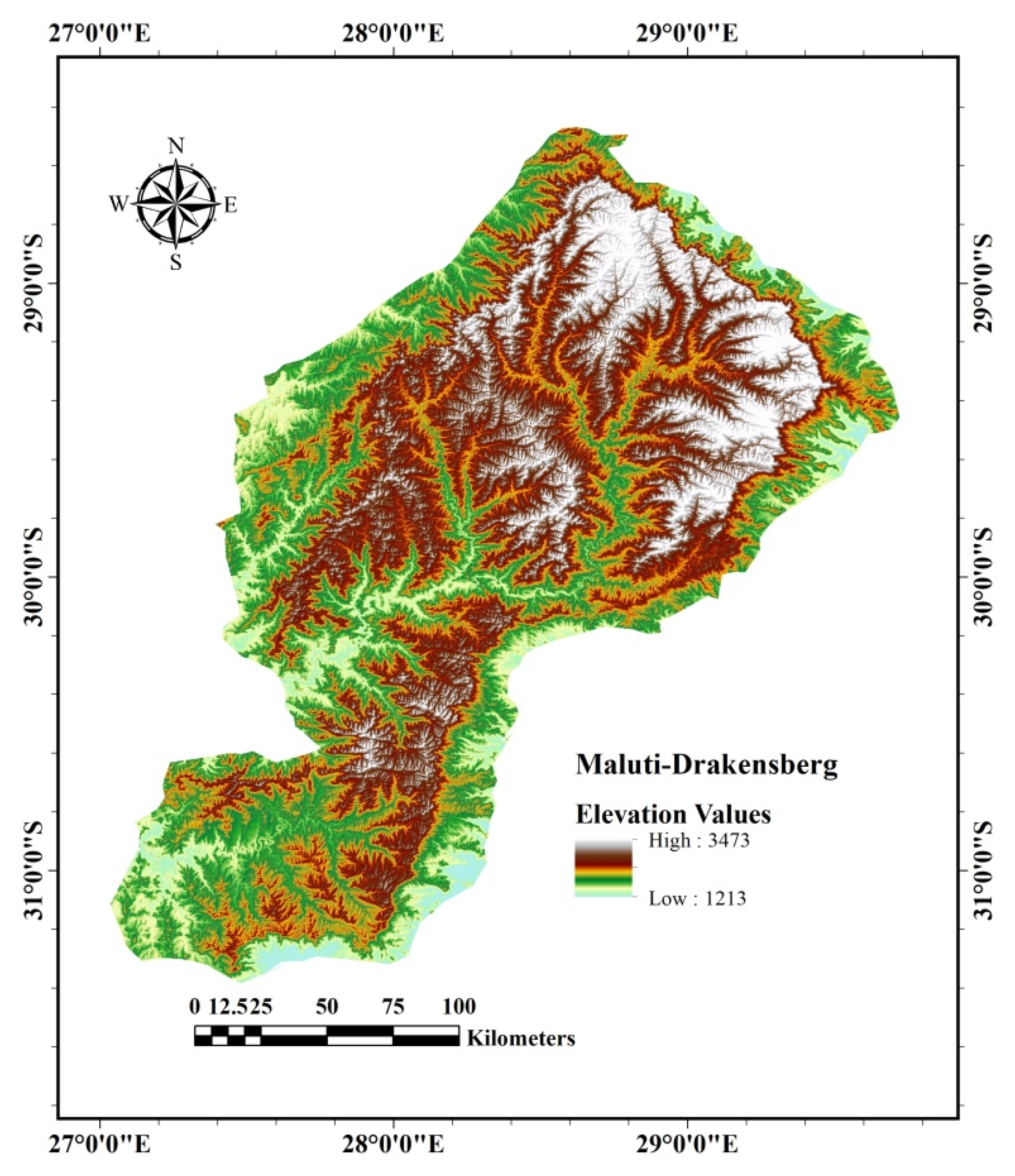
Figure 2.
Annual average maximum temperature for the period 1960–2016.
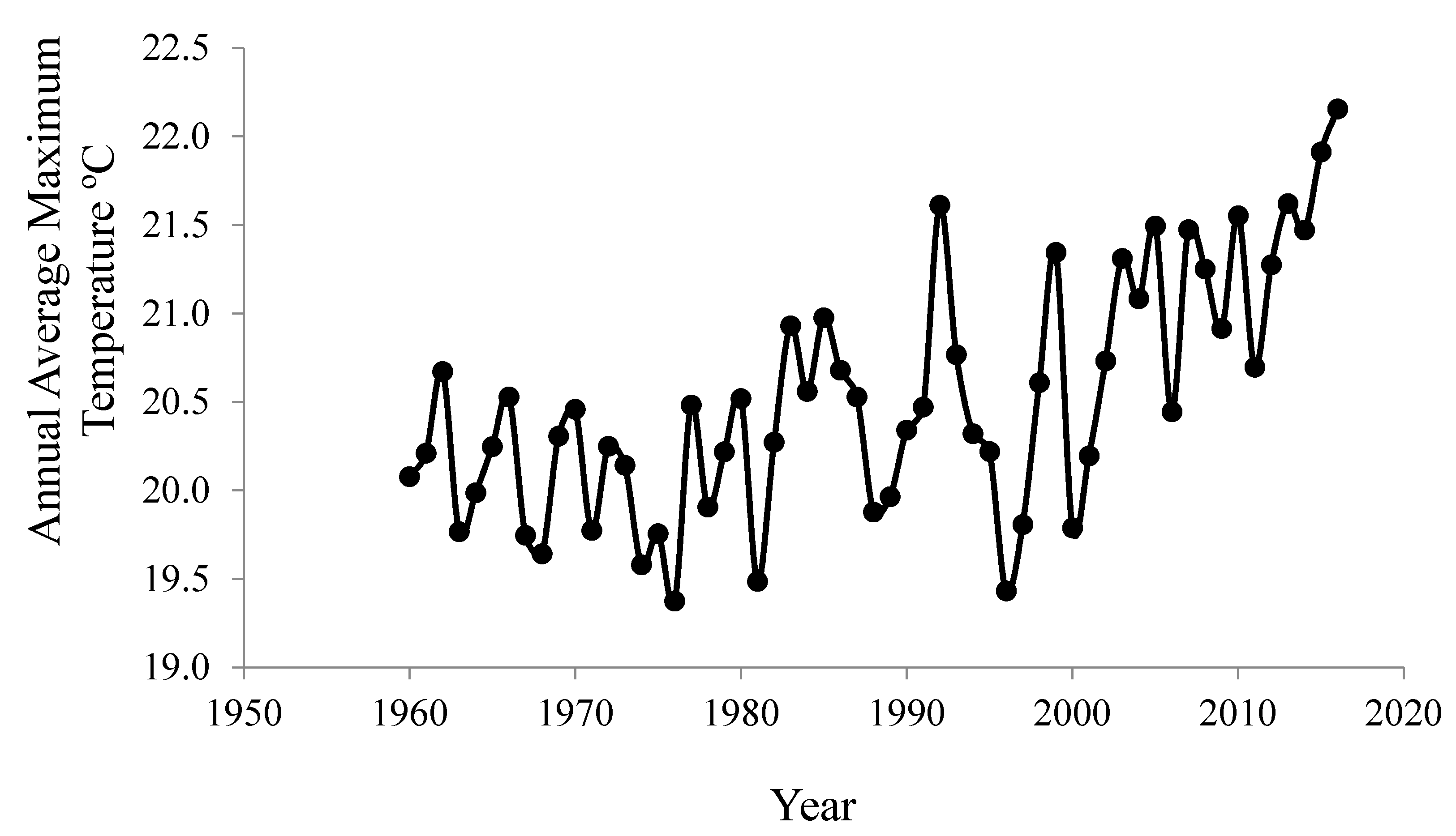
Figure 3.
Annual average minimum temperature for the period 1960–2016.

Figure 4.
Lowess regression line for the annual average maximum temperature of Maloti-Drakensberg for the period 1960–2016.
Figure 4.
Lowess regression line for the annual average maximum temperature of Maloti-Drakensberg for the period 1960–2016.

Figure 5.
Lowess regression line for the annual average minimum temperature of Maloti-Drakensberg for the period 1960–2016.
Figure 5.
Lowess regression line for the annual average minimum temperature of Maloti-Drakensberg for the period 1960–2016.

Figure 6.
Mann–Kendall and linear regression slopes of annual average maximum temperature for Maloti-Drakensberg for the period of 1960–2016.
Figure 6.
Mann–Kendall and linear regression slopes of annual average maximum temperature for Maloti-Drakensberg for the period of 1960–2016.

Figure 7.
Mann–Kendall and linear regression slopes of season, October–December (OND), annual average maximum temperature for Maloti-Drakensberg for the period of 1960–2016.
Figure 7.
Mann–Kendall and linear regression slopes of season, October–December (OND), annual average maximum temperature for Maloti-Drakensberg for the period of 1960–2016.

Figure 8.
Mann–Kendall and linear regression slopes of annual average minimum temperature for Maloti-Drakensberg for the period of 1960–2016.
Figure 8.
Mann–Kendall and linear regression slopes of annual average minimum temperature for Maloti-Drakensberg for the period of 1960–2016.
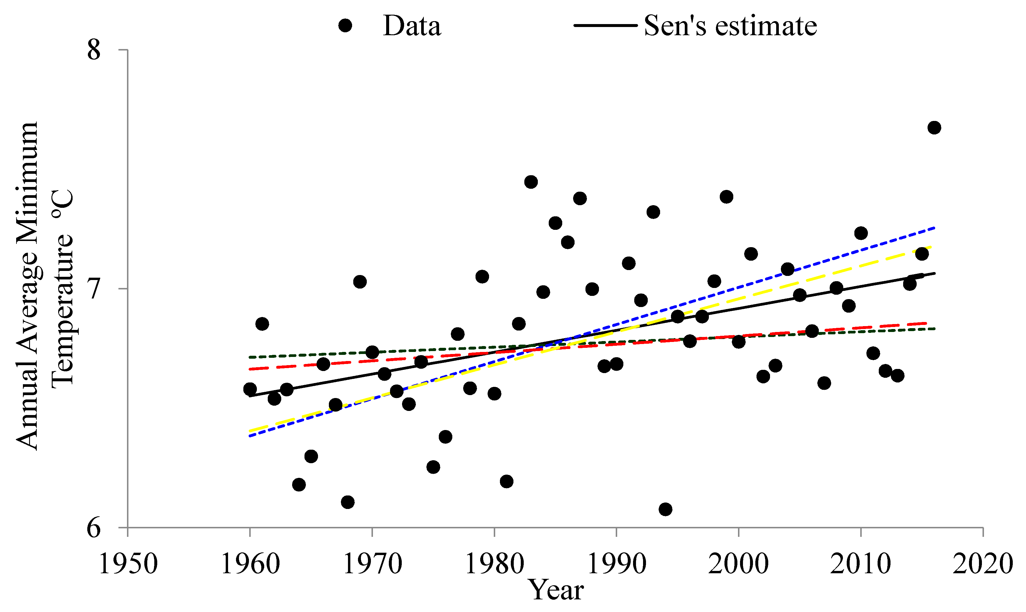
Figure 9.
Mann–Kendall and linear regression slopes of season OND annual average minimum temperature for Maloti-Drakensberg for the period of 1960–2016.
Figure 9.
Mann–Kendall and linear regression slopes of season OND annual average minimum temperature for Maloti-Drakensberg for the period of 1960–2016.
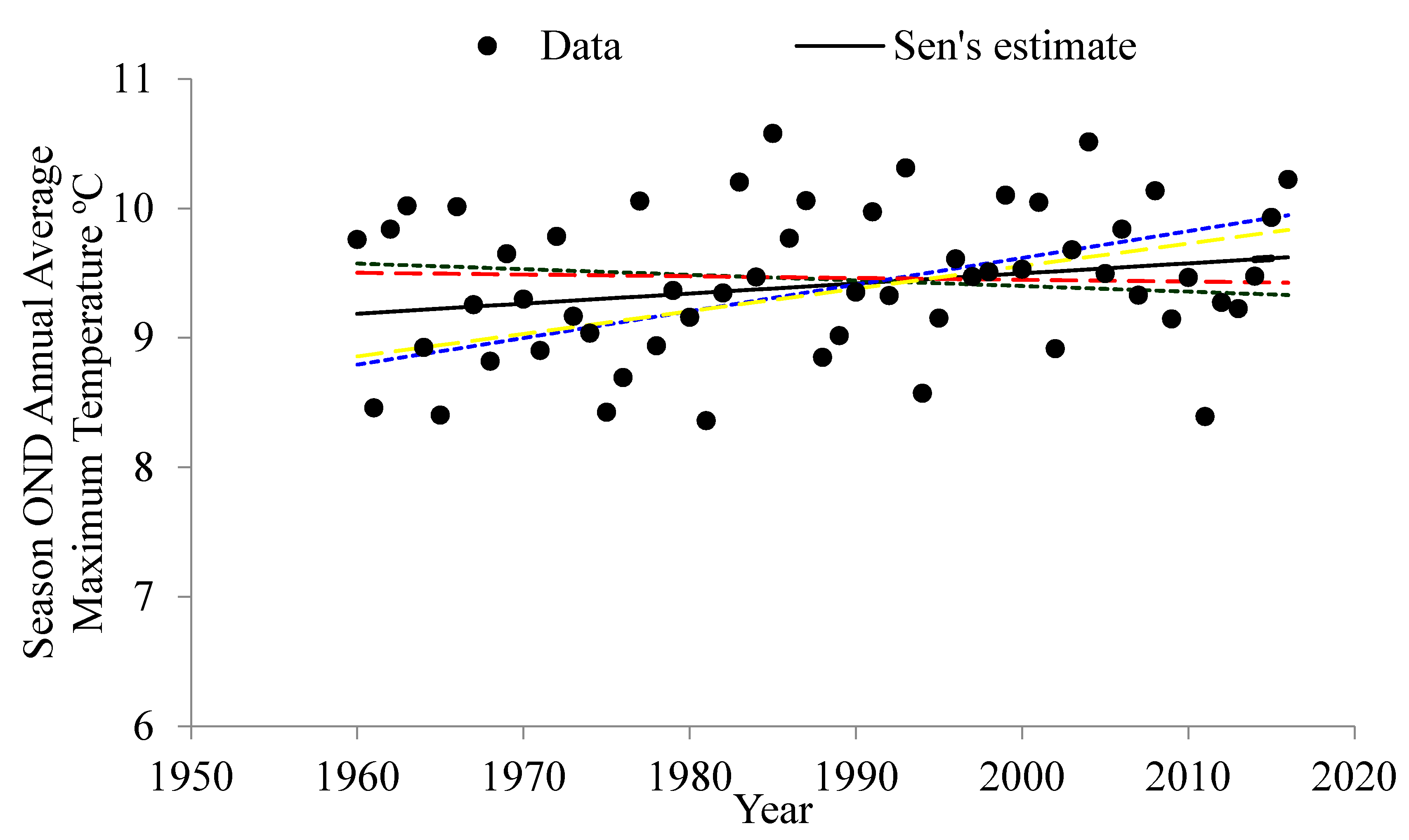
Figure 10.
Red line in the upper diagram is the stepwise trend showing regime shifts in the mean of the annual average maximum temperature detected by the sequential t-test for analyzing regime shift (STARS) method; black solid bars in the lower diagram are the RSI magnitude.
Figure 10.
Red line in the upper diagram is the stepwise trend showing regime shifts in the mean of the annual average maximum temperature detected by the sequential t-test for analyzing regime shift (STARS) method; black solid bars in the lower diagram are the RSI magnitude.
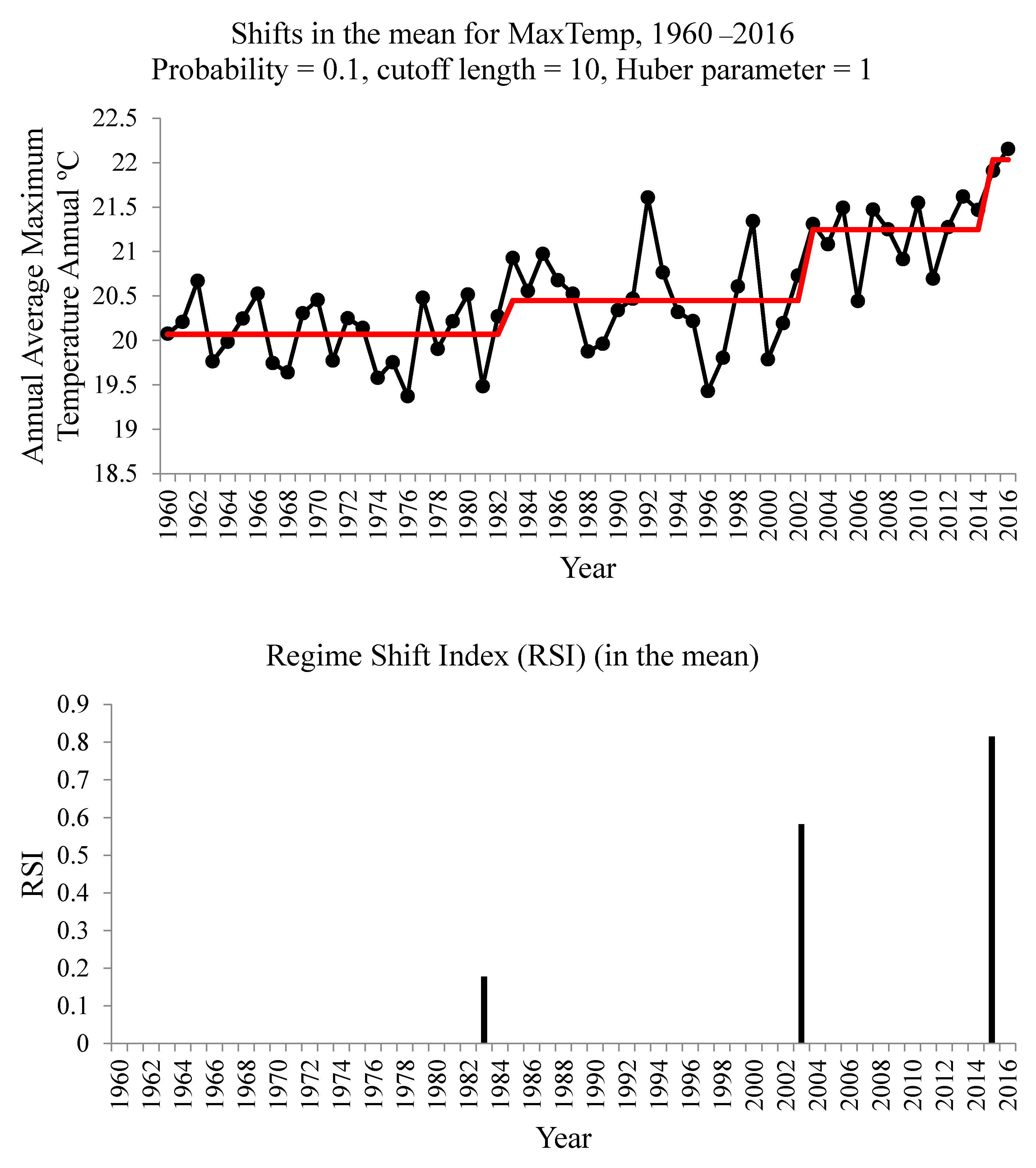
Figure 11.
Red line in the upper diagram is the stepwise trend showing regime shifts in the mean of the annual average minimum temperature detected by the STARS method; black solid bars in the lower diagram are the RSI magnitude.
Figure 11.
Red line in the upper diagram is the stepwise trend showing regime shifts in the mean of the annual average minimum temperature detected by the STARS method; black solid bars in the lower diagram are the RSI magnitude.

Table 1.
Annual average maximum temperature summary statistics.
| Statistic Description | Temperature Data |
|---|---|
| Amount of data | 57 |
| Maximum value | 22.15 |
| Minimum value | 19.37 |
| Sum | 1169.18 |
| Mean | 20.51 |
| Std.error | 0.09 |
| Variance | 0.45 |
| Stand. Dev Median Skewness Kurtosis Coeff. Var | 0.67 20.46 0.44 –0.49 3.28% |
Table 2.
Annual average minimum temperature summary statistics.
| Statistic Description | Temperature Data |
|---|---|
| Amount of data | 57 |
| Maximum value | 7.67 |
| Minimum value | 6.08 |
| Sum | 388 |
| Mean | 6.81 |
| Std.error | 0.05 |
| Variance | 0.12 |
| Stand. Dev Median Skewness Kurtosis Coeff. Var | 0.35 6.78 0.05 –0.08 5.1% |
Table 3.
Annual average maximum temperature trend analysis.
| Mann–Kendall Trend | Sen’s Slope Estimate | ||||||||||||||
|---|---|---|---|---|---|---|---|---|---|---|---|---|---|---|---|
| Time Series | Start Year | End Year | N | Test Z | Significance | Q | Qmin99 | Qmax99 | Qmin95 | Qmax95 | B | Bmin99 | Bmax99 | Bmin95 | Bmax95 |
| January | 1960 | 2016 | 57 | 2.58 | + | 0.018 | −0.010 | 0.044 | −0.003 | 0.038 | 24.93 | 25.45 | 24.35 | 25.31 | 24.52 |
| February | 1960 | 2016 | 57 | 2.66 | ** | 0.031 | 0.001 | 0.061 | 0.009 | 0.054 | 23.50 | 24.43 | 22.70 | 24.36 | 22.82 |
| March | 1960 | 2016 | 57 | 0.92 | ** | 0.035 | 0.003 | 0.063 | 0.010 | 0.055 | 21.97 | 22.89 | 21.11 | 22.61 | 21.38 |
| April | 1960 | 2016 | 57 | 1.58 | ** | 0.038 | 0.008 | 0.067 | 0.016 | 0.060 | 18.68 | 19.52 | 17.85 | 19.33 | 17.96 |
| May | 1960 | 2016 | 57 | 3.21 | *** | 0.048 | 0.027 | 0.067 | 0.033 | 0.061 | 15.81 | 16.32 | 15.38 | 16.19 | 15.57 |
| June | 1960 | 2016 | 57 | 2.02 | *** | 0.031 | 0.012 | 0.052 | 0.018 | 0.048 | 13.92 | 14.50 | 13.34 | 14.40 | 13.44 |
| July | 1960 | 2016 | 57 | 0.90 | * | 0.017 | −0.003 | 0.041 | 0.003 | 0.035 | 14.64 | 15.24 | 14.16 | 15.04 | 14.33 |
| August | 1960 | 2016 | 57 | 1.08 | * | 0.023 | 0.000 | 0.048 | 0.006 | 0.042 | 16.56 | 17.20 | 15.91 | 17.06 | 15.96 |
| September | 1960 | 2016 | 57 | −0.32 | + | 0.019 | −0.006 | 0.045 | 0.000 | 0.038 | 19.94 | 20.56 | 19.20 | 20.48 | 19.39 |
| October | 1960 | 2016 | 57 | 1.15 | *** | 0.030 | 0.008 | 0.058 | 0.013 | 0.052 | 20.73 | 21.30 | 19.7178 | 21.093 | 19.9275 |
| November | 1960 | 2016 | 57 | −0.12 | ** | 0.022 | 0.000 | 0.042 | 0.005 | 0.037 | 22.156 | 22.6259 | 21.581 | 22.626 | 21.6809 |
| December | 1960 | 2016 | 57 | 1.99 | 0.008 | −0.016 | 0.032 | −0.011 | 0.025 | 24.189 | 24.7835 | 23.6275 | 24.597 | 23.724 | |
| ANNUAL | 1960 | 2016 | 57 | 3.34 | *** | 0.026 | 0.015 | 0.038 | 0.018 | 0.035 | 19.881 | 20.1143 | 19.4974 | 20.032 | 19.5687 |
| OND | 1960 | 2016 | 57 | 1.63 | ** | 0.019 | 0.004 | 0.035 | 0.008 | 0.031 | 22.46 | 22.8045 | 21.9308 | 22.728 | 22.0821 |
*** if trend at α = 0.001 level of significance; ** if trend at α = 0.01 level of significance; * if trend at α = 0.05 level of significance; + if trend at α = 0.1 level of significance; If the cell is blank, the significance level is greater than 0.1.
Table 4.
Annual average minimum temperature trend analysis.
| Mann–Kendall Trend | Sen’s Slope Estimate | ||||||||||||||
|---|---|---|---|---|---|---|---|---|---|---|---|---|---|---|---|
| Time Series | Start Year | End Year | N | Test Z | Significance | Q | Qmin99 | Qmax99 | Qmin95 | Qmax95 | B | Bmin99 | Bmax99 | Bmin95 | Bmax95 |
| January | 1960 | 2016 | 57 | 2.58 | ** | 0.014 | 0.000 | 0.028 | 0.004 | 0.025 | 12.10 | 12.55 | 11.83 | 12.44 | 11.87 |
| February | 1960 | 2016 | 57 | 2.66 | ** | 0.018 | 0.001 | 0.033 | 0.005 | 0.030 | 11.66 | 12.08 | 11.31 | 11.99 | 11.37 |
| March | 1960 | 2016 | 57 | 0.92 | 0.007 | −0.011 | 0.024 | −0.006 | 0.021 | 10.45 | 11.12 | 9.88 | 10.95 | 10.00 | |
| April | 1960 | 2016 | 57 | 1.58 | 0.015 | −0.010 | 0.033 | −0.003 | 0.028 | 6.56 | 7.26 | 6.04 | 7.02 | 6.09 | |
| May | 1960 | 2016 | 57 | 3.21 | ** | 0.021 | 0.004 | 0.039 | 0.010 | 0.035 | 2.69 | 3.14 | 2.12 | 3.06 | 2.23 |
| June | 1960 | 2016 | 57 | 2.02 | * | 0.014 | −0.005 | 0.032 | 0.000 | 0.027 | −0.29 | 0.22 | −0.83 | 0.15 | −0.65 |
| July | 1960 | 2016 | 57 | 0.90 | 0.008 | −0.013 | 0.027 | −0.008 | 0.023 | −0.15 | 0.35 | −0.59 | 0.24 | −0.50 | |
| August | 1960 | 2016 | 57 | 1.08 | 0.009 | −0.013 | 0.027 | −0.007 | 0.023 | 1.94 | 2.50 | 1.24 | 2.36 | 1.40 | |
| September | 1960 | 2016 | 57 | −0.32 | −0.003 | −0.023 | 0.017 | −0.018 | 0.011 | 5.53 | 6.09 | 4.91 | 5.93 | 5.16 | |
| October | 1960 | 2016 | 57 | 1.15 | 0.009 | −0.011 | 0.030 | −0.006 | 0.024 | 7.59 | 8.13 | 6.89293 | 7.9534 | 7.05845 | |
| November | 1960 | 2016 | 57 | −0.12 | −0.001 | −0.017 | 0.015 | −0.014 | 0.011 | 9.4359 | 9.86805 | 9.01978 | 9.7777 | 9.10037 | |
| December | 1960 | 2016 | 57 | 1.99 | * | 0.010 | −0.003 | 0.024 | 0.000 | 0.021 | 10.833 | 11.232 | 10.4194 | 11.125 | 10.4911 |
| ANNUAL | 1960 | 2016 | 57 | 3.34 | *** | 0.009 | 0.002 | 0.016 | 0.003 | 0.014 | 6.5524 | 6.7152 | 6.3862 | 6.6624 | 6.40689 |
| OND | 1960 | 2016 | 57 | 1.63 | 0.008 | −0.004 | 0.021 | −0.001 | 0.017 | 9.192 | 9.5759 | 8.79038 | 9.5068 | 8.85775 | |
*** if trend at α = 0.001 level of significance; ** if trend at α = 0.01 level of significance; * if trend at α = 0.05 level of significance; + if trend at α = 0.1 level of significance; If the cell is blank, the significance level is greater than 0.1.
© 2019 by the authors. Licensee MDPI, Basel, Switzerland. This article is an open access article distributed under the terms and conditions of the Creative Commons Attribution (CC BY) license (http://creativecommons.org/licenses/by/4.0/).
Share and Cite
MDPI and ACS Style
Mohamed, A.A.; Mukwada, G. Temperature Changes in the Maloti-Drakensberg Region: An Analysis of Trends for the 1960–2016 Period. Atmosphere 2019, 10, 471. https://doi.org/10.3390/atmos10080471
AMA Style
Mohamed AA, Mukwada G. Temperature Changes in the Maloti-Drakensberg Region: An Analysis of Trends for the 1960–2016 Period. Atmosphere. 2019; 10(8):471. https://doi.org/10.3390/atmos10080471
Chicago/Turabian StyleMohamed, Abdelmoneim Abdelsalam, and Geoffrey Mukwada. 2019. "Temperature Changes in the Maloti-Drakensberg Region: An Analysis of Trends for the 1960–2016 Period" Atmosphere 10, no. 8: 471. https://doi.org/10.3390/atmos10080471
Note that from the first issue of 2016, this journal uses article numbers instead of page numbers. See further details here.