Projections of Alpine Snow-Cover in a High-Resolution Climate Simulation
by
 , , , ,
Samuel Lüthi
1 ,
,
Nikolina Ban
1,*,†,
Sven Kotlarski
2,
Christian R. Steger
1,
Tobias Jonas
3 and
Christoph Schär
1 1
Institute for Atmospheric and Climate Sciences, ETH Zürich, 8006 Zurich, Switzerland
2
Federal Office of Meteorology and Climatology, MeteoSwiss, Zurich Airport, 8058 Zurich, Switzerland
3
WSL Institute for Snow and Avalanche Research SLF, 7260 Davos, Switzerland
*
Author to whom correspondence should be addressed.
†
Current address: Universitaetsstr. 16, 8092 Zürich, Switzerland.
Atmosphere 2019, 10(8), 463; https://doi.org/10.3390/atmos10080463
Submission received: 15 July 2019
/
Revised: 29 July 2019
/
Accepted: 1 August 2019
/
Published: 13 August 2019
(This article belongs to the Special Issue Cryosphere in and around Regional Climate Models)
Abstract
:The recent development of high-resolution climate models offers a promising approach in improving the simulation of precipitation, clouds and temperature. However, higher grid spacing is also a promising feature to improve the simulation of snow cover. In particular, it provides a refined representation of topography and allows for an explicit simulation of convective precipitation processes. In this study we analyze the snow cover in a set of decade-long high-resolution climate simulation with horizontal grid spacing of 2.2 km over the greater Alpine region. Results are compared against observations and lower resolution models (12 and 50 km), which use parameterized convection. The simulations are integrated using the COSMO (Consortium for Small-Scale Modeling) model. The evaluation of snow water equivalent (SWE) in the simulation of present-day climate, driven by the ERA-Interim reanalysis, against an observational dataset, reveals that the high-resolution simulation clearly outperforms simulations with grid spacing of 12 and 50 km. The latter simulations underestimate the cumulative amount of SWE over Switzerland over the whole annual cycle by 33% (12 km simulation) and 56% (50 km simulation) while the high-resolution simulation shows a spatially and temporally averaged difference of less than 1%. Scenario simulations driven by GCM MPI-ESM-LR (2081–2090 RCP8.5 vs. 1991–2000) reveal a strong decrease of SWE over the Alps, consistent with previous studies. Previous studies had found that the relative decrease becomes gradually smaller with elevation, but this finding was limited to low and intermediate altitudes (as a 12 km simulation resolves the topography up to 2500 m). In the current study we find that the height gradient reverses sign, and relative reductions in snow cover increases above 3000 m asl, where important parts of the cryosphere are present. In addition, the simulations project a transition from permanent to seasonal snow cover at high altitudes, with potentially important impacts to Alpine permafrost. This transition and the more pronounced decline of SWE emphasize the value of the higher grid spacing. Overall, we show that high-resolution climate models offer a promising approach in improving the simulation of snow cover in Alpine terrain.
1. Introduction
Snow cover in the Northern Hemisphere has significantly decreased since the middle of the 20th century [1]. This decrease was around 1.6% per decade for March and April and 11.7% for June over the period from 1967–2012. Also, permafrost temperatures have been increasing in most regions of the Northern Hemisphere since the 1980s, which led to reductions in permafrost thickness and spatial extent [1]. This trend is projected to further increase [1]. Consistent with these hemispheric trends, Alpine snow cover showed marked decreases. Even though snow depth, duration of continuous snow cover, and number of snowfall days increased gradually from the 1930s until the early 1980s, these indicators significantly decreased towards the end of the century [2]. This observed reduction can be attributed to the increased temperature since changes in precipitation remained rather small [3]. This trend is more pronounced at lower elevations, where winter temperatures are generally closer to the melting point. By the end of the century, Alpine snow volumes are projected to drop by 90%, 50%, and 30% for altitudes of 1000 m, 2000 m, and 3000 m, respectively [4]. In a recent study using an ensemble of regional climate models (RCMs), results show a reduction of 40–80% by mid-century for sites below 1500 m under an SRES A1B emission scenario [5]. For elevations between 2000–2500 m, reductions amount to 10–60% by mid-century and 30–80% by the end of the century, depending upon the model considered. This decrease leads to strong changes in the Alpine snow climate and poses major ecological and socio-economic challenges. Snow cover is an important part of the Alpine climate system as it alters surface energy fluxes by isolating the underlying ground through its comparably low thermal conductivity. More importantly, it increases the surface albedo which cools the surface by backscattering shortwave radiation. This highly non-linear snow-albedo feedback is one of the most important positive feedbacks in the climate system [6]. For ecology, snow cover is essential as not only the seasonal vegetation cycle but also hibernating animals depend strongly on the timing of the snow season [7]. Especially in the Alps, snow cover plays also a major economic role. Factors such as the length of the snow season or the snow reliability are crucial for the profitability of Alpine tourist destinations [8]. Moreover, snow functions as a key storage of water for hydropower, which accounts for more than half of the Swiss electricity production [9]. As an additional effect, declining snow cover and melting of permafrost can lead to new areas being affected by landslides and rock-fall hazards [10].
Thanks to the increase in the computational power in recent years, high-resolution regional climate models—models with horizontal resolutions of 1–4 km—are being used for climate change simulations [11,12,13,14]. The higher resolution allows to switch off the parametrization for convection, thereby enabling an improved representation of clouds and moist convection. In addition, higher resolution allows a better representation of complex mountainous topography. This aspect is especially promising for the simulation of snow, as previous studies concluded that the capability of climate models in simulating snow cover is considerably limited due to their horizontal resolution [5,15,16]. A higher resolution allows to better capture topographically influenced processes, such as winter inversions and cold air pools that are relevant for snow preservation. In the Alps, a higher grid spacing also allows to represent elevation levels above 3000 m, nearly up to 4000 m. This is a major advantage, as the climate change impact on the cryosphere depends considerably on surface elevation [17], and substantial parts of snow, permafrost and glaciers are present at high elevations.
Up to now, most of the studies using high-resolution models focused on precipitation and clouds, and little research was conducted for snow, especially over Europe. Based on these identified gaps, we here address the following research questions:
- Do kilometer–scale regional climate simulations provide an added value in terms of snow cover representation in Alpine terrain?
- How is Alpine snow cover expected to change by the end of the 21st century based on high resolution regional climate simulations?
To answer these questions, we use the set of simulations presented in [11,12] and previously analyzed for precipitation, but not for snow. The following section gives an overview of data sets and the different model runs. In Section 3.1 we are assessing the added value of higher horizontal resolution in simulating snow by comparing observational data of snow water equivalents (SWE) against three runs of the same model using different grid spacings (2.2 km, 12 km, and 50 km). In Section 3.2, we analyze the climate change signal of Alpine SWE, snowfall and temperatures and we assess the influence of horizontal grid spacing. Finally, we discuss our results in Section 3.4 and conclude the study in Section 4.
2. Data and Methods
2.1. Model Data
The model data utilised for this study encompasses output from several existing simulations of the non-hydrostatic COSMO model (Consortium for Small-Scale Modeling) [18,19,20]. Details of the model set-up may be looked up in Ban et al. [11] while here only a brief overview of the main features is presented.
The COSMO model is designed for limited-area weather forecasts and for regional climate simulations (i.e., for the application as an RCM) at horizontal resolutions from 0.5 to 200 km. The small grid scale of the 2.2 km resolution allows to resolve deep convection explicitly. In the 12 km and the 50 km model experiment, convection is parameterized using the Tiedtke mass-flux scheme with moisture convergence closure [21]. Time steps of 90 and 300 s are applied for the 12 and the 50 km simulation, respectively, while for the 2.2 km simulation a temporal discretization of 20 s is used. The model is horizontally discretized on a rotated latitude-longitude grid. Vertically, a pressure-based hybrid coordinate with 60 levels is used (40 levels for the 50 km simulation). The levels range from the surface to the top of the atmosphere at 20 hPa and have a vertical grid spacing from 20 m near the surface up to 1.2 km at the top.
In the COSMO model, snow is represented as a single layer whose mass budget is determined by snowfall, sublimation, runoff and soil infiltration. Drifting snow, which leads to lateral redistribution and typically enhances sublimation, is not considered in the model. Likewise, retention of surface meltwater or rainfall within the snowpack by refreezing or as irreducible water in temperate snow is neglected. The fractional snow coverage of a grid cell is parameterized as a linear function of the snow water equivalent. Snow density is restricted to a range of 50–400 kg m−3 and changes due to compaction and snow metamorphism, which is assumed to be a function of snow temperature, and accumulation of fresh snow. Snow albedo varies in the range of 0.4 to 0.7 and decreases linearly, which represents the aging of snow, and increases with snowfall accumulation. The snow albedo for forest-covered grid cells is computed as an area-weighted mean of the open-area snow albedo and the constant albedo-values for deciduous and evergreen forest [22].
Due to computational costs, the 2.2 km simulation covers only the greater Alpine region, whereas the 12 and the 50 km simulations cover almost entire Europe. Figure 1 shows the analysis domain of this study and the capability of the three simulations in representing the orography. As customary in high-resolution climate modelling, all simulations are only run for a ten-year period due to the high computational costs. As a consequence, natural variability plays a more important factor than in traditional climate simulations where usually 20–30 year periods are considered. The simulations are run over three different time periods. Table 1 summarizes the various simulations and model properties. The period from 1998–2007 is used to evaluate the model with the respective observational data sets. Furthermore, the 2.2 and the 12 km simulation are run over a control period from 1991–2000 and a scenario period from 2081–2090, assuming the RCP8.5 scenario for greenhouse gas concentrations. For the evaluation period, the simulations are driven by lateral boundary conditions from the ERA–Interim reanalysis. During the control and the scenario period, the boundary conditions for the 12 km simulation are provided by the global climate model MPI-ESM-LR [23]. For all periods the 2.2 km simulation is driven by the respective 12 km simulation. We hence employ a double one-way nesting procedure: the 12 km simulation is driven by reanalysis data and global model output at the lateral boundaries (Era-Interim or MPI-ESM-LR) and, in turn, provides boundary forcing for the nested 2.2 km experiment. The 50 km experiment is directly driven by Era-Interim (see Table 1). For more information on the rationale behind regional climate modelling and on the respective nesting techniques we refer to the recent work by Giorgi [24].
In order to properly spin-up the soil-moisture, the 12 km simulations have been initialized 5 years and the 2.2 km simulation 2 months, prior to the analysis periods (i.e., the first 5 years or 2 months, respectively, are discarded for the analysis). As the snow cover may accumulate the climate effects of past years, it is also important to briefly discuss how snow is initialized. When the 2.2 km simulations are initialized, data for snow cover, soil moisture and soil temperature are provided by the respective point in time of the driving 12 km simulation (which uses an extended spin-up period). Note that, as the vertical range of topography reaches higher up in the 2.2 km simulation, the snow at very high altitudes will not be initialized realistically. Also, the snow model lacks a glacier module, i.e., there is no transformation from snow to firn and permanent ice, and there are no lateral ice fluxes. To investigate the sensitivity of our analysis to the applied modeling strategy, we have monitored the snow-cover evolution over the entire duration of the simulations. Even for the highest altitude range considered in our study (3000–3500 m), spin-up effect are seen only in the first two years, and will thus not significantly affect the main results.
2.2. Observational Data
Validation of the simulated snow cover was performed with observational data from 203 stations of the Swiss national snow monitoring networks. To allow direct comparison of these data to results from the various RCM simulations, the station data were mapped to each model orography individually following Steger et al. [5]. The mapping involved four steps:
- First, measured snow depth data were converted to SWE using a snow density model based on methods presented by Martinec and Rango [25]. This model describes accumulation and densification of the snowpack layer by layer. Here, we used a recalibrated version of their original model using data from over 10,000 snow profiles presented in Jonas et al. [26].
- Then, for each day, the station data was detrended allowing non-linear SWE profiles.
- Next, the detrended SWE values were interpolated to the model orography using a 3-dimensional Gaussian filter weighting approach described in Jrg-Hess et al. [27]. Optimized filter widths were identified using a leave-one-out validation approach.
- Finally, a subgrid scaling was applied to account for the influence of topography on snow distribution and redistribution in mountainous terrain. To this end, slope- and aspect-dependent correction functions were trained using a set of high-resolution snow depth maps from airborne lidar acquisitions in the European Alps as presented in Grünewald et al. [28], and applied at a 25 m spatial resolution.
This procedure ensured that the final SWE grids accurately represent areal mean snow amount from measurements obtained on flat field sites. Note, however, that due to the improved representation of higher elevations with increasing horizontal resolution and the predominantly positive SWE-elevation-gradients, the spatially averaged SWE amount is much larger in the 2.2 km and the 12 km observational reference than in the 50 km counterpart.
In an application using a 1 km orography [29], the above approach was shown to produce SWE grids that were highly consistent with independent satellite observations of snow cover fraction. While the monitoring sites were generally well distributed in space, stations were, however, considerable sparser at elevations above 2700 m asl. Given the non-linear height dependence of SWE, observational data on high elevation levels are therefore subject to large uncertainties. This is a common issue on high elevation levels [30,31,32]. Also, many stations—typically those in Swiss winter tourism destinations—are shut down during the summer period. This leads to a smaller data availability during the summer months which reduces the data quality. Therefore, data for August and September had to be excluded from the evaluation.
Furthermore, model validation could only be performed for Switzerland since the SWE reference data were restricted to that area. Nevertheless, Hantel and Hirtl-Wielke [33] have shown that snow cover sensitivities are similar throughout the whole Alps. Hence, we assume that the results from our model validation are transferable to an Alpine-wide range, given that the topography of Switzerland covers nearly the whole Alpine elevation range.
2.3. Methods
As outlined above, we here present both an evaluation and a climate change analysis. Model evaluation assesses the capability of the simulations in representing historical SWE in Switzerland as represented by the observational data set. For this purpose the RCM is driven by ERA-Interim data and the simulations cover the ten year time period from 1998–2007. For the evaluation we focus mainly on the spatial pattern, the annual cycle and the elevation profile of SWE. As mentioned in Section 2.2, insufficient observations are available during August and September. Thus, these two months had to be excluded from the evaluation.
The climate change analysis focuses on SWE changes over the Greater Alpine region between the 10 year control period 1991–2000 (CTRL) and the scenario period 2081–2090 (SCEN) assuming the RCP8.5 emission scenario and only employing the 2.2 and 12 km horizontal resolutions. Both the CTRL and the SCEN run are driven by lateral boundary conditions from the global climate model MPI-ESM-LR. Note that due to the fact that only ten-year long periods are considered, internal climate variability could in principle contribute to the identified climate change signals. However, 12 km simulations are also available for extended 30-year periods (1976–2005 and 2071–2100), and comparison reveals similar climate-change signals in terms of temperature and precipitation changes [12]. We thus expect that the short integration period has only a minor effect on the projections. In addition, the assessment of resolution effects is not affected by the duration of the simulations.
To a large part, the analysis has been performed by investigating absolute differences, both for the evaluation and the climate change analysis. However, to also investigate relative differences, cumulative SWE values have been used (Figures 3 and 6) or thresholds have been applied (Figure 5) to limit the effects of small SWE values. To quantify the climate change impact, percentage changes (Figures 8 and 9) and absolute differences (Figure 10) have been used.
3. Results
3.1. Evaluation of Snow Water Equivalent
3.1.1. Seasonal Mean Snow Water Equivalent
The spatial pattern of seasonal means for the three simulations and observations at 2.2 km resolution over Switzerland is shown in Figure 2. We here show the 2.2 km version of the observational reference as this version includes most of the topographic details and likely best reflects the true SWE distribution. ERA@2 shows a realistic spatial snow distribution with high values of SWE in the center of the Alps and lower values within the valleys and the Swiss plateau. While ERA@12 indicates higher SWE values over the Alpine ridge, ERA@50 simulates a too homogeneous spatial distribution over Switzerland. The more realistic pattern of ERA@2 can be explained by its more detailed representation of topography, which is the same topography as used for constructing the 2.2 km observational reference dataset (see Section 2.2). ERA@12 and especially ERA@50 show smaller values than ERA@2. This is due to the fact that the 2.2 km simulation has more grid-points at higher elevation levels, and thus better represents temperatures below the melting point, while the 12 km and especially the 50 km simulation do not reach high enough to simulate sub-zero temperatures for much of the year. This affects especially the topographically more complex Alpine area, and explains the generally lower SWE values for ERA@12 and especially ERA@50. ERA@2 shows a large bias in the central Alpine domain compared to the observations. This bias is partly explained by the large uncertainties of the observational data at high elevation levels, but also by the known overestimation of precipitation of high-resolution models at high altitudes [11,12]. However, ERA@2 keeps higher amounts of SWE even during the summer months, which is closer to reality than the interpolated data from the observational data set. This is also confirmed by Hantel et al. [34] who located the median Alpine summer snow line for the time horizon 1961–2010 at 3100 m asl. At the coarser grid spacings (simulated and observed), Switzerland is completely snow free during summer.
3.1.2. Annual Cycle of Snow Water Equivalent
The annual cycle of SWE (Figure 3), shows that ERA@2 is able to reproduce the 2.2 km observations well. As observed, the average amount of SWE peaks in early March before the melting period starts. However, the model shows earlier onset of snow during autumn and early winter and earlier melting in spring. The earlier melting in spring could be partially explained by the neglect of refreezing or storage of liquid water in the snow pack [35]. This process is not accounted for in the COSMO snow model but plays an important role in reality. The plateau of SWE levels from March until May is a result of continuous accumulation of snow at high elevation levels and melting at lower elevation. As ERA@12 and ERA@50 have fewer grid points at high altitudes, the two simulations are less capable to simulate this plateau effect.
While ERA@12 is still capable in reproducing the shape of the annual cycle of the observations at the 12 km scale, ERA@50 shows large differences. Both underestimate the average SWE amount substantially throughout the whole snow season. Also, both simulations reveal a too early snow ablation in spring, which results in a nearly snow free Switzerland by early May and early June for ERA@50 and ERA@12, respectively. In terms of the average cumulative amount of SWE (Figure 3 middle and bottom), ERA@2 shows a remarkable performance with less than one percentage difference by the end of the annual cycle. ERA@12 and ERA@50 underestimate the average cumulative amount by roughly the same absolute amount which leads to a relative bias of −33% and −56%, respectively.
3.1.3. Height Profile of Snow Water Equivalent
Figure 4 shows the vertical profile of SWE for the three simulations and observations over Switzerland. The vertical profile of SWE is calculated as an average across grid points that are within the same 100 m elevation band. One key advantage of the smaller grid spacing becomes obvious: the smaller the grid spacing, the better the resolution of the Alpine elevation profile (see Figure 4, right-hand panel). In the simulation with the 2.2 km grid-spacing, elevations up to nearly 4000 m asl are present, while the highest grid-point for the 12 and the 50 km simulation are at 2958 and 2102 m asl, respectively.
While all three simulations are capable of representing the observational values during DJF and ON, larger biases occur during MAM and JJ, especially for ERA@12 and ERA@50. The large MAM biases of nearly one order of magnitude can be linked to the premature ablation of snow. On the other hand, the small biases in autumn might be favoured by the early onset of snow, that compensates for the general underestimation of SWE in these simulations. As previously touched on in Section 3.1, ERA@2 shows very large SWE amounts at elevations above 2500 m. Again, this large difference is presumably not only a result of the known overestimation of precipitation at high altitudes (and, hence, of winter snow accumulation), but also due to the large uncertainties of the observational data set at these high elevation levels.
3.2. Climate Change Signal of Alpine Snow Water Equivalents
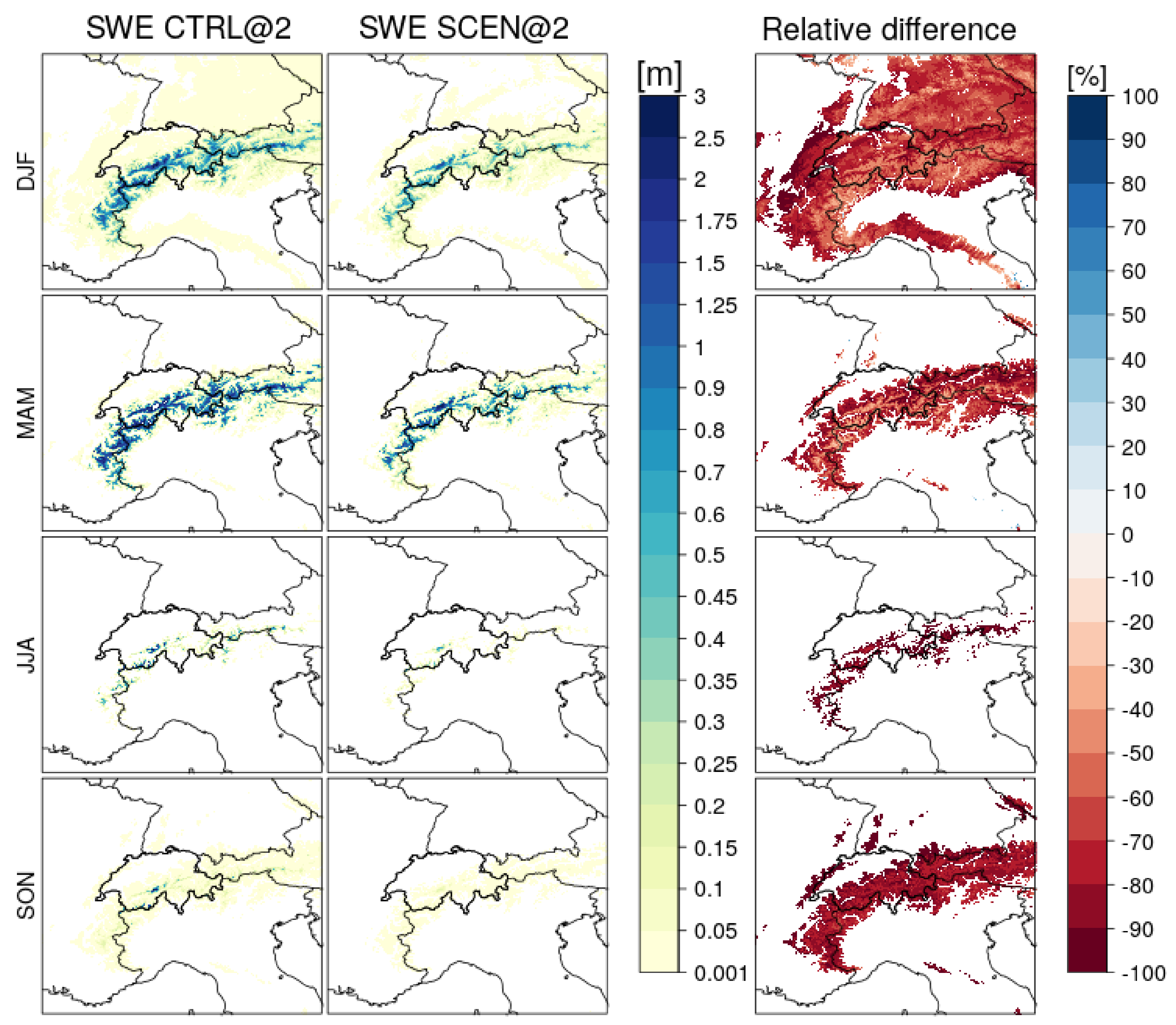
In this section we present the projected future changes in snow water equivalent over the greater Alpine region. The change of seasonal mean SWE is shown in Figure 5. On average over the whole year, SWE amounts decrease by roughly 60% in the Alpine region. During DJF, the Alps experience a decrease of SWE by 40–60%. The relative decrease is more pronounced in lower regions and valleys (around −80% in the Rhone and the Rhine valley) than at higher elevation levels (around −40 to −50%). The MAM period looks similar to the DJF period. Again, the largest relative decrease (close to −100%) occurs in the lower regions around the Alpine arch. Similar to DJF the relative SWE decrease is smaller at higher elevations (−40 to −60%). During JJA, relative changes for most of the grid points that have snow during the CTRL period are close to −100%. Only very high grid points keep some snow throughout the summer which might partly be related to the missing representation of a dedicated glacier module in the COSMO model (see Section 2.1). Finally, the relative decrease of −100% in most parts of the analyzed domain during SON can be associated with the later onset of snow under warmer climatic conditions (see Section 3.2.1).
3.2.1. Annual Cycle of Snow Water Equivalent in a Warmer Climate
The annual cycle of SWE for the two different simulations, averaged over the analysis domain, is shown in Figure 6. It can be seen that the annual cycle of SWE undergoes two major changes. Not only is the average SWE amount considerably smaller throughout the whole cycle, but also the snow season is shortened by roughly two months (top panel). Average autumn SWE values from CTRL are reached a month later in SCEN, while average spring values are reached a month earlier. The mid-season values from CTRL are not nearly reached in SCEN. The only similarity is the form of the cycle. For both simulation periods, snow accumulates until early March before the melting starts. Cumulatively, SCEN@12 shows much lower SWE values than SCEN@2 (mid panel). However, both simulations show an average cumulative decrease of 60% for the domain over the whole year (bottom panel).
Changes in the annual cycle on high elevation levels are displayed in Figure 7. While changes in the range of 2000 to 2500 and 2500 to 3000 m asl resemble the change to the overall cycle, the most remarkable change takes place at elevations between 3000 and 3500 m asl (Figure 7, top). At this elevation range, snow cover persists during the whole annual cycle during the CTRL period. However, the ascending zero-degree level leads to a complete melting of snow during the SCEN period in summer and fall. This implies a loss of permanent snow cover throughout most of the Alpine terrain. Only the high-resolution simulation is capable to simulate this major impact on the cryosphere. This impressively highlights the utility of such simulations.
3.2.2. Projected Changes in the Vertical Profile of Snow Water Equivalent
A direct consequence of the underlying warming in the RCP8.5 scenario is the ascent of the zero-degree level. Thus, for all four seasons, SWE values from the CTRL period are found 300–500 m higher up in the SCEN period. The shift is smaller in the snow intense seasons DJF and MAM. To further assess the changes in the vertical profile of SWE, we consider in Figure 8 the seasonal-mean SWE as a function of height. In this analysis we focus on “fresh snow”, as there are some spin-up effects at high elevations with permanent snow cover (i.e., the permanent snow cover is growing during the first 1–2 years of CTRL@2, see Section 2.1). More specifically we subtract the SWE level at the 1st of October from the whole cycle of the respective hydrological year when assessing relative changes of SWE in the vertical profile.
The relative reduction of fresh SWE from SCEN compared to CTRL is more pronounced during DJF than during MAM and JJA (Figure 8). This can be linked to the general later onset of snow. The two simulations agree very closely with the relative decrease throughout the whole elevation range of the 12 km simulation (thus up to 3000 m asl). As expected, the relative reduction becomes smaller with height. However, above 3000 m asl, the decrease is more pronounced as a linear extrapolation of the trend between 2000 and 3000 m asl would suggest. This effect is even more intense if the loss of permanent (perennial) snow would be included in the analysis. Again, only the high-resolution simulation is capable to simulate this non-linear profile.
3.3. Projected Changes in the Vertical Profile of Temperature and Snowfall
In order to explain the non-linear behavior in changes of vertical profile of SWE, we analyze vertical profiles of snowfall and temperature (Figure 9 and Figure 10). Unfortunately, we do not have an observational dataset for the evaluation of snowfall for the 2.2 km simulation. Thus, the confidence in the model’s capability in simulating realistic snowfall patterns on 2.2 km comes from (I) its strong performance in simulating SWE, temperature, and precipitation and (II) its previously evaluated performance on the 12 km simulation [36]. The evaluation for precipitation and temperature has been done in previous studies already [11,12,37].
The changes in snowfall look similar to the changes in SWE but are less pronounced. On average over the whole year, snowfall amounts drop by roughly 40% (SWE drop by 60%). The snowfall decrease is smallest at high elevations during winter. Even in a warmer climate, most precipitation will be falling as snow at these high elevation levels, as temperature will mostly stay below zero degrees. The changes in the annual cycle of snowfall (not shown) look similar to those of SWE. The domain average amount is considerably lower throughout the whole annual cycle during the SCEN period. Autumn levels of snowfall from the CTRL period are only reached in mid winter in SCEN, while the peak CTRL levels during winter are not reached at all. As seen before for SWE, this contributes to a shortening of the snow season by roughly two months. Nonetheless, the peak of the annual cycle of snowfall remains in mid February for both periods.
Looking at the elevation profile, snowfall amounts from the CTRL period can be found 300–500 m higher up in the SCEN period for DJF and MAM (Figure 9). This change is larger for JJA and SON. The snowfall amounts decrease by less than 20% above 2000 m (DJF) and 2500 m (MAM). This is a considerably smaller decrease compared to the decline of SWE. Also, the relative decline of snowfall becomes gradually smaller with elevation and thus does not show the non-linear behavior seen with SWE. The largest changes occur in JJA, where snow fall decreases by almost 70% even at the highest elevations.
Snowfall and SWE amounts depend strongly on the temperature profile (Figure 10), and in particular on changes of the zero-degree level. The warming is stronger during JJA and SON with an increase in temperature of 4–6 °C compared to a warming of 2–4 °C during DJF and MAM. Interestingly, the warming is more pronounced on higher elevation levels during all four seasons. This is a fundamental aspect of climate change in general and associated with large-scale increases in atmospheric lapse-rate [38] and also evident evident on a larger scale (Europe) [17,39,40]. As a consequence of this enhanced upper-level warming, the ascent of the zero-degree line in SCEN is more pronounced on higher elevation level. This ascent is more pronounced during JJA and SON (>900 m and 800 m respectively) than for DJF and MAM (400 m and 600 m respectively), which can be explained by the differences in the seasonal warming rates. During JJA, the seasonal average zero-degree level rises from about 3000 to close to 4000 m asl. Hence, even the highest grid points will regularly experience positive temperatures and thus melting of snow during summer. In addition to the large-scale changes in lapse-rate (see above), this can also be linked to the snow-albedo feedback that partially explains the stronger warming at high altitudes [41].
3.4. Discussion
The model evaluation presented in Section 3.1 has revealed that the 2.2 km simulation outperforms the simulations with coarser grid-spacing in reproducing the annual cycle of snow-water equivalent (SWE). Even though it shows a premature onset of SWE in autumn and a premature melting in spring, it is capable of reproducing the annual cycle well. The seasonal peak of SWE in early March is accurately reproduced by the model and the cumulative amount of SWE over the whole year is simulated with less than a percentage difference to the observational data set. This small number, however, likely results to some extent from an error compensation when averaging SWE over space (Switzerland) and time (winter season). While the 12 km simulation is still capable in reproducing the shape of the annual cycle, the 50 km simulation struggles. Also, both coarse-resolution simulations, 50 and 12 km, substantially underestimate the amount of SWE throughout the whole year. This leads to a cumulative underestimation of SWE amounts by 33% for 12 km and 56% for 50 km simulation. The 2 km simulation considerably overestimates SWE values at high elevation levels. This can partly be explained by large uncertainties of observations at these elevations, but also by the known overestimation of precipitation in convection-resolving models at high altitudes [11].
A comparison of the model output between the control period and the scenario period largely reveals agreement between the 2 km and the 12 km simulation. The strongest relative decrease in SWE can be expected in autumn, which can be linked to the later onset of snow. Besides the later onset in autumn, the melting in spring will start earlier. This leads to a shortening of the snow season by roughly two months. Nevertheless, the peak values of SWE remain at the beginning of March, and do not shift to an earlier time in winter as suggested by Steger et al. [5].
The most prominent change to the annual cycle takes place above 3000 m asl. At this elevation range snow cover can persist during the whole annual cycle during the control period. However, the ascending zero-degree level leads to a nearly complete melting of snow during the scenario period in summer. This implies a loss of permanent snow cover throughout most of the Alpine terrain. The changes in SWE above 3000 m can only be seen in the 2.2 km model, which due to its higher resolution, is able to represent these altitudes. This is especially important since the highest SWE amounts and important parts of the cryosphere can be found in this elevation range. Overall, cumulative annual SWE amounts drop by 60% in this altitude range, which is in line with Steger et al. [5].
Snowfall amounts in the analyzed domain are expected to decrease by 40%. This decrease is smallest at elevation levels above 2000 m during winter (<20%). In contrast to SWE, the relative decline of snowfall becomes gradually smaller with elevation. These results are consistent with the recent work by Frei et al. [36]. The increase in temperature is projected to be larger during summer and autumn than during winter and spring. Also, the ascent of the zero-degree level of roughly 800 m is larger during summer than in spring and winter (400 m). For all seasons, the warming is projected to be more intense at higher elevations. This leads to mean summer temperatures above the melting point up to elevations of 4000 m asl.
4. Conclusions
Previous work have shown that high-resolution regional climate models offer a promising approach towards improving the quality of temperature and precipitation projections [11,12,13,37,42]. Besides the ability of high-resolution models to explicitly resolve convective cloud and precipitation systems, the better resolution of topography is a promising feature to also improve the simulation of snow cover [15,16]. In this study we have analyzed the evolution of the Alpine snow cover for a convection-resolving model with a 2.2 km horizontal grid spacing and compared it to convection-parameterizing simulations with grid spacings of 12 km and 50 km. In the first part of the study, the simulated snow cover was evaluated against an observational data set. In the second part, we investigated the change of snow cover in a warmer climate by comparing the scenario period (2081–2090) against the control period (1991–2000) under the RCP8.5 emission scenario. Additionally, we performed a brief analysis of the associated changes in Alpine snowfall and temperature.
Referring to the research objectives stated in Section 1 and extending previous work on high-resolution regional climate modelling towards snow cover representation, we conclude that:
- High resolution climate simulations are a promising tool to improve the simulation of Alpine snow cover. They clearly outperform simulations with grid spacings of 12 km and 50 km in representing the annual cycle of SWE. Also, thanks to the better representation of topography, the high resolution simulations can represent snow cover on high elevation levels where snow may be present even during the summer months.
- Under climate change, Alpine snow cover amounts are expected to drop by 60% in the high resolution simulation. This result is in line with the literature and simulations with larger grid spacing (12 km). However, the high resolution climate simulation allows to analyse changes above 3000 m asl, where a loss of perennial snow cover can be expected.
- Overall, the high-resolution climate model approach is especially promising for regions with complex topography and at high elevations.
Author Contributions
S.L. analyzed the data and wrote the paper; N.B. performed simulations at 12 and 2.2 km; S.K. performed simulations at 50 km; C.R.S. contributed with analysis tools; T.J. provided the observational data; C.S. contributed to the set-up of the simulations, the interpretation of the results, and the write-up of the paper. All authors commented on the paper.
Funding
Funding for this study has been provided by the Swiss National Science Foundation through grant 200021-132614 and Sinergia grant CRSII2-154486/1 crCLIM. We also acknowledge PRACE for awarding us access to Piz Daint at CSCS, Switzerland, where the simulations have been conducted.
Acknowledgments
We acknowledge the Federal Office for Meteorology and Climatology MeteoSwiss, the Swiss National Supercomputing Centre (CSCS), and ETH Zurich for their contributions to the development of the GPU-accelerated version of COSMO. We further thank the three anonymous reviewers for their comments.
Conflicts of Interest
The authors declare no conflict of interest.
References
- Stocker, T.F.; Qin, D.; Plattner, G.K.; Tignor, M.; Allen, S.K.; Boschung, J.; Nauels, A.; Xia, Y.; Bex, V.; Midgley, P.M.; et al. Climate Change 2013: The Physical Science Basis; Cambridge University Press: Cambridge, UK, 2013. [Google Scholar]
- Laternser, M.; Schneebeli, M. Long-term snow climate trends of the Swiss Alps (1931–99). Int. J. Climatol. 2003, 23, 733–750. [Google Scholar] [CrossRef]
- Scherrer, S.C.; Appenzeller, C.; Laternser, M. Trends in Swiss Alpine snow days: The role of local-and large-scale climate variability. Geophys. Res. Lett. 2004, 31. [Google Scholar] [CrossRef]
- Beniston, M.; Keller, F.; Koffi, B.; Goyette, S. Estimates of snow accumulation and volume in the Swiss Alps under changing climatic conditions. Theor. Appl. Climatol. 2003, 76, 125–140. [Google Scholar] [CrossRef] [Green Version]
- Steger, C.; Kotlarski, S.; Jonas, T.; Schär, C. Alpine snow cover in a changing climate: A regional climate model perspective. Clim. Dyn. 2013, 41, 735–754. [Google Scholar] [CrossRef]
- Scherrer, S.; Ceppi, P.; Croci-Maspoli, M.; Appenzeller, C. Snow-albedo feedback and Swiss spring temperature trends. Theor. Appl. Climatol. 2012, 110, 509–516. [Google Scholar] [CrossRef]
- Marchand, P.J. Life in the Cold: An Introduction to Winter Ecology; UPNE: Hanover, NH, USA, 2014. [Google Scholar]
- Elsasser, H.; Abegg, B.; Buerki, R. Climate change and winter sports: Environmental and economic threats. Geogr. Bull. 2006, 38, 26. [Google Scholar]
- Swiss Federal Office of Energy SFOE. Hydropower; SFOE: Bern, Switzerland, 2018. [Google Scholar]
- Voigt, T.; Füssel, H.M.; Gärtner-Roer, I.; Huggel, C.; Marty, C.; Zemp, M. Impacts of Climate Change on Snow, Ice, and Permafrost in Europe: Observed Trends, Future Projections, and Socio-Economic Relevance; European Topic Centre on Air and Climate Change: Bilthoven, The Netherlands, 2010. [Google Scholar]
- Ban, N.; Schmidli, J.; Schär, C. Evaluation of the convection-resolving regional climate modeling approach in decade-long simulations. J. Geophys. Res. Atmos. 2014, 119, 7889–7907. [Google Scholar] [CrossRef]
- Ban, N.; Schmidli, J.; Schär, C. Heavy precipitation in a changing climate: Does short-term summer precipitation increase faster? Geophys. Res. Lett. 2015, 42, 1165–1172. [Google Scholar] [CrossRef]
- Kendon, E.J.; Roberts, N.M.; Senior, C.A.; Roberts, M.J. Realism of rainfall in a very high-resolution regional climate model. J. Clim. 2012, 25, 5791–5806. [Google Scholar] [CrossRef]
- Coppola, E.; Sobolowski, S.; Pichelli, E.; Raffaele, F.; Ahrens, B.; Anders, I.; Ban, N.; Bastin, S.; Belda, M.; Belusic, D.; et al. A first-of-its-kind multi-model convection permitting ensemble for investigating convective phenomena over Europe and the Mediterranean. Clim. Dyn. 2017, 1–32. [Google Scholar] [CrossRef]
- Dutra, E.; Kotlarski, S.; Viterbo, P.; Balsamo, G.; Miranda, P.M.; Schär, C.; Bissolli, P.; Jonas, T. Snow cover sensitivity to horizontal resolution, parameterizations, and atmospheric forcing in a land surface model. J. Geophys. Res. Atmos. 2011, 116, D21109. [Google Scholar] [CrossRef]
- Rasmussen, R.; Liu, C.; Ikeda, K.; Gochis, D.; Yates, D.; Chen, F.; Tewari, M.; Barlage, M.; Dudhia, J.; Yu, W.; et al. High-resolution coupled climate runoff simulations of seasonal snowfall over Colorado: A process study of current and warmer climate. J. Clim. 2011, 24, 3015–3048. [Google Scholar] [CrossRef]
- Kotlarski, S.; Bosshard, T.; Lüthi, D.; Pall, P.; Schär, C. Elevation gradients of European climate change in the regional climate model COSMO-CLM. Clim. Chang. 2012, 112, 189–215. [Google Scholar] [CrossRef]
- Steppeler, J.; Doms, G.; Schättler, U.; Bitzer, H.; Gassmann, A.; Damrath, U.; Gregoric, G. Meso-gamma scale forecasts using the nonhydrostatic model LM. Meteorol. Atmos. Phys. 2003, 82, 75–96. [Google Scholar] [CrossRef]
- Doms, G.; Förstner, J. Development of a kilometer-scale NWP-system: LMK. COSMO Newsl. 2004, 4, 159–167. [Google Scholar]
- Baldauf, M.; Seifert, A.; Förstner, J.; Majewski, D.; Raschendorfer, M.; Reinhardt, T. Operational Convection-Scale Numerical Weather Prediction with the COSMO Model: Description and sensitivities. Mon. Weather Rev. 2011, 139, 3887–3905. [Google Scholar] [CrossRef]
- Tiedtke, M. A comprehensive mass flux scheme for cumulus parameterization in large-scale models. Mon. Weather. Rev. 1989, 117, 1779–1800. [Google Scholar] [CrossRef]
- Doms, G.; Förstner, J.; Heise, E.; Herzog, H.; Mironov, D.; Raschendorfer, M.; Reinhardt, T.; Ritter, B.; Schrodin, R.; Schulz, J.P.; et al. A Description of the Nonhydrostatic Regional COSMO Model. Part II: Physical Parameterization; Deutscher Wetterdienst: Offenbach, Germany, 2011. [Google Scholar]
- Stevens, B.; Giorgetta, M.; Esch, M.; Mauritsen, T.; Crueger, T.; Rast, S.; Salzmann, M.; Schmidt, H.; Bader, J.; Block, K.; et al. Atmospheric component of the MPI-M Earth System Model: ECHAM6. J. Adv. Model. Earth Syst. 2013, 5, 146–172. [Google Scholar] [CrossRef]
- Giorgi, F. Thirty Years of Regional Climate Modeling: Where Are We and Where Are We Going next? J. Geophys. Res. 2019, 124, 5696–5723. [Google Scholar] [CrossRef]
- Martinec, J.; Rango, A. Indirect evaluation of snow reserves in mountain basins. IAHS Publ. 1991, 205, 111–119. [Google Scholar]
- Jonas, T.; Marty, C.; Magnusson, J. Estimating the snow water equivalent from snow depth measurements in the Swiss Alps. J. Hydrol. 2009, 378, 161–167. [Google Scholar] [CrossRef]
- Jörg-Hess, S.; Griessinger, N.; Zappa, M. Probabilistic forecasts of snow water equivalent and runoff in mountainous areas. J. Hydrometeorol. 2015, 16, 2169–2186. [Google Scholar] [CrossRef]
- Grünewald, T.; Bühler, Y.; Lehning, M. Elevation dependency of mountain snow depth. Cryosphere 2014, 8, 2381–2394. [Google Scholar] [CrossRef] [Green Version]
- Hüsler, F.; Jonas, T.; Riffler, M.; Musial, J.P.; Wunderle, S. A satellite-based snow cover climatology (1985–2011) for the European Alps derived from AVHRR data. Cryosphere 2014, 8, 73–90. [Google Scholar] [CrossRef]
- Bales, R.; Dressler, K.; Imam, B.; Fassnacht, S.; Lampkin, D. Fractional snow cover in the Colorado and Rio Grande basins, 1995–2002. Water Resour. Res. 2008, 44. [Google Scholar] [CrossRef]
- Fassnacht, S.; Dressler, K.; Bales, R. Snow water equivalent interpolation for the Colorado River Basin from snow telemetry (SNOTEL) data. Water Resour. Res. 2003, 39. [Google Scholar] [CrossRef] [Green Version]
- Fassnacht, S.; Dressler, K.; Hultstrand, D.; Bales, R.; Patterson, G. Temporal inconsistencies in coarse-scale snow water equivalent patterns: Colorado River Basin snow telemetry-topography regressions. Pirineos 2012, 165–185. [Google Scholar] [CrossRef]
- Hantel, M.; Hirtl-Wielke, L.M. Sensitivity of Alpine snow cover to European temperature. Int. J. Climatol. 2007, 27, 1265–1275. [Google Scholar] [CrossRef]
- Hantel, M.; Maurer, C.; Mayer, D. The snowline climate of the Alps 1961–2010. Theor. Appl. Climatol. 2012, 110, 517–537. [Google Scholar] [CrossRef]
- Kuhn, M.; Helfricht, K.; Ortner, M.; Landmann, J.; Gurgiser, W. Liquid water storage in snow and ice in 86 Eastern Alpine basins and its changes from 1970–97 to 1998–2006. Ann. Glaciol. 2016, 57, 11–18. [Google Scholar] [CrossRef]
- Frei, P.; Kotlarski, S.; Liniger, M.A.; Schär, C. Snowfall in the Alps: Evaluation and projections based on the EURO-CORDEX regional climate models. Cryosphere 2018, 2018, 1–24. [Google Scholar] [CrossRef]
- Heim, C. Daily Temperature Variability in Convection-Resolving Climate Simulations. Master’s Thesis, IAC ETHZ, Zurich, Switzerland, 2015. [Google Scholar]
- Santer, B.D.; Wigley, T.M.; Mears, C.; Wentz, F.J.; Klein, S.A.; Seidel, D.J.; Taylor, K.E.; Thorne, P.W.; Wehner, M.F.; Gleckler, P.J.; et al. Amplification of surface temperature trends and variability in the tropical atmosphere. Science 2005, 309, 1551–1556. [Google Scholar] [CrossRef]
- Kotlarski, S.; Lüthi, D.; Schär, C. The elevation dependency of 21st century European climate change: An RCM ensemble perspective. Int. J. Climatol. 2015, 35, 3902–3920. [Google Scholar] [CrossRef]
- Brogli, R.; Kröner, N.; Sørland, S.L.; Lüthi, D.; Schär, C. The Role of Hadley Circulation and Lapse-Rate Changes for the Future European Summer Climate. J. Clim. 2019, 32, 385–404. [Google Scholar] [CrossRef]
- Winter, K.J.P.M.; Kotlarski, S.; Scherrer, S.C.; Schär, C. The Alpine snow-albedo feedback in regional climate models. Clim. Dyn. 2017, 48, 1109–1124. [Google Scholar] [CrossRef]
- Kendon, E.J.; Roberts, N.M.; Fowler, H.J.; Roberts, M.J.; Chan, S.C.; Senior, C.A. Heavier summer downpours with climate change revealed by weather forecast resolution model. Nat. Clim. Chang. 2014, 4, 570. [Google Scholar] [CrossRef]
Figure 1.
Analysis domain and representation of topography (m) for the simulations with horizontal grid spacings of 50 km (left), 12 km (middle), and 2.2 km (right). The analysis domain ranges from 2.5° E/42.5° N to 16.8° E/49.6° N.
Figure 1.
Analysis domain and representation of topography (m) for the simulations with horizontal grid spacings of 50 km (left), 12 km (middle), and 2.2 km (right). The analysis domain ranges from 2.5° E/42.5° N to 16.8° E/49.6° N.

Figure 2.
Seasonal mean snow water equivalent over the area of Switzerland during the evaluation period 1998–2007. Results are shown for the three COSMO simulations (driven by ERA-interim lateral boundary conditions) with grid spacings of 50 km (left column), 12 km (center-left), and 2.2 km (center-right) and observations interpolated to the 2.2 km gird (right column).

Figure 3.
Annual cycle of snow water equivalent averaged over Switzerland. Results are presented for the three horizontal resolutions 2.2 km (dark blue), 12 km (light blue), and 50 km (orange) for the model output (dashed lines) and the observations (solid lines). Displayed are mean SWE (top), cumulative SWE (middle), and the relative difference of the cumulative SWE of the simulations to the respective observations ((ERA-OBS)/OBS; bottom).

Figure 4.
Vertical profile of seasonal mean SWE (left-hand four panels) and number of model grid-points, representing the area-elevation distribution at the respective horizontal resolution (right). The SWE values are calculated as averages of grid-points over Switzerland that lie within the same 100 m elevation bands. The gray shading at the top levels indicates the uncertainties of SWE estimates due to the limited number (<10) of grid points per bin in OBS@2.

Figure 5.
Projected changes of SWE over the Alpine region. Displayed are the seasonal average values of the CTRL period (1991–2000, first column) and the SCEN period (2081–2090, center). The relative difference (right column) is expressed as the difference between SCEN and CTRL simulations, normalized by CTRL. Relative differences are only displayed if a threshold of 1 mm SWE is exceeded during the CTRL period.

Figure 6.
Projected changes in the annual cycle of Alpine SWE averaged over the analysis domain (see Figure 1). Results are shown for the mean SWE (top), cumulative SWE (middle), and the relative difference between the SCEN (2081–2090, dashed line) and the CTRL (1991–2000, full line) period (bottom) for the 2.2 km (dark blue) and the 12 km (light blue) simulations.

Figure 7.
Projected changes in the annual cycle of Alpine SWE at high elevations. Results are shown for the mean SWE in the height range of 3000–3500 (top), 2500–3000 (middle), and 2000–2500 m asl (bottom) for the SCEN (2081–2090, dashed line) and the CTRL (1991–2000, full line) period for the 2.2 km (dark blue) and the 12 km (light blue) simulations.

Figure 8.
Vertical profile of projected changes of fresh seasonal-mean SWE. Changes are expressed as the difference of seasonal averages between the SCEN (2081–2090) and the CTRL (1991–2000) period normalized by CTRL for the 2.2 km (dark blue) and the 12 km (light blue) simulations (first four columns). The right-hand plot shows the number of grid points per 100 m bin in the analysis area. In contrast to the other figures, the underlying SWE values are corrected for permanent snow (see text for details). The gray shading on the highest elevation levels indicate larger uncertainties due to the limited number (<10) of grid-points per bin in the 2-km simulations.

Figure 9.
Vertical profile of seasonal-mean snowfall (kg m−2 d−1) during the SCEN (2081–2090, dashed lines) and the CTRL (1991–2000, full line) periods (top row) and associated relative changes of snowfall (bottom row). Snowfall values are shown as the average snowfall of grid-points that lie within the same 100 m elevation band for the 2.2 km (dark blue) and the 12 km (light blue) simulation. Relative changes (bottom row) are expressed as the difference of seasonal averages between the SCEN (2081–2090) and the CTRL (1991–2000) period normalized by CTRL. The gray shading at the highest elevation levels indicates the larger uncertainties due to the limited number (<10) of grid-points per bin in the 2.2 km simulations.

Figure 10.
Vertical profile of average seasonal 2m temperature (°C) during the SCEN (2081–2090, dashed lines) and the CTRL (1991–2000, full line) period for the 2.2 km (dark blue) and the 12 km (light blue) simulations (top row), and climate change signal of the vertical warming profile (bottom row). The climate change signal is expressed as the difference of seasonal averages between the SCEN (2081–2090) and the CTRL (1991–2000) period for the 2 km (dark blue) and the 12 km (light blue) simulations.


Table 1.
Details of the simulation data used in this study.
| Model Run | Period | Time | Driving Data | (km) | (s) | Deep Convection | # Grid Points in Analysis Area | # Grid Points above 2000 m | Highest Grid Point (m asl) |
|---|---|---|---|---|---|---|---|---|---|
| ERA@50 | Evaluation | 1998–2007 | Era-Interim | 50 | 300 | Tiedtke | 651 (31 × 25) | 2 | 2102 |
| ERA@12 | Evaluation | 1998–2007 | Era-Interim | 12 | 90 | Tiedtke | 7676 | 188 | 2958 |
| CTRL@12 | Control | 1991–2000 | MPI-ESM-LR | (101 × 76) | |||||
| SCEN@12 | Scenario | 2081–2090 | MPI-ESM-LR (RCP8.5) | ||||||
| ERA@2 | Evaluation | 1998–2007 | ERA@12 km | 2.2 | 20 | Explicit | 161,236 | 6796 | 3944 |
| CTRL@2 | Control | 1991–2000 | CTRL@12 km | (466 × 346) | |||||
| SCEN@2 | Scenario | 2081–2090 | SCEN@12 |
© 2019 by the authors. Licensee MDPI, Basel, Switzerland. This article is an open access article distributed under the terms and conditions of the Creative Commons Attribution (CC BY) license (http://creativecommons.org/licenses/by/4.0/).
Share and Cite
MDPI and ACS Style
Lüthi, S.; Ban, N.; Kotlarski, S.; Steger, C.R.; Jonas, T.; Schär, C. Projections of Alpine Snow-Cover in a High-Resolution Climate Simulation. Atmosphere 2019, 10, 463. https://doi.org/10.3390/atmos10080463
AMA Style
Lüthi S, Ban N, Kotlarski S, Steger CR, Jonas T, Schär C. Projections of Alpine Snow-Cover in a High-Resolution Climate Simulation. Atmosphere. 2019; 10(8):463. https://doi.org/10.3390/atmos10080463
Chicago/Turabian StyleLüthi, Samuel, Nikolina Ban, Sven Kotlarski, Christian R. Steger, Tobias Jonas, and Christoph Schär. 2019. "Projections of Alpine Snow-Cover in a High-Resolution Climate Simulation" Atmosphere 10, no. 8: 463. https://doi.org/10.3390/atmos10080463
Note that from the first issue of 2016, this journal uses article numbers instead of page numbers. See further details here.