Large-Eddy Simulations of Oil Droplet Aerosol Transport in the Marine Atmospheric Boundary Layer

Abstract

In this study, a hybrid large-eddy simulation (LES) model is developed and applied to simulate the transport of oil droplet aerosols in wind over progressive water waves. The LES model employs a hybrid spectral and finite difference method for simulating the wind turbulence and a bounded finite-volume method for modeling the oil aerosol transport. Using a wave-following coordinate system and computational grid, the LES model captures the turbulent flow and oil aerosol fields in the region adjacent to the unsteady wave surface. A flat-surface case with prescribed roughness (representing a pure wind-sea) and a wavy-surface case with regular plane progressive 100 m long waves (representing long-crest long-wavelength ocean swells) are considered to illustrate the capability of the LES model and study the effects of long progressive waves on the transport of oil droplet aerosols with four different droplet diameters. The simulation results and statistical analysis reveal enhanced suspension of oil droplets in wind turbulence due to strong disturbance from the long progressive waves. The spatial distribution of the aerosol concentration also exhibits considerable streamwise variations that correlate with the phase of the long progressive waves.

1. Introduction

In the aftermath of an offshore oil spill accident, the spilled crude oil can stay on the ocean surface for a long period of time before being restored. During this period, frequently-occurring events at the sea surface, such as wave breaking and bubble burst, can generate a considerable amount of small aerosolized oil droplets [1], which can then be further transported upward and downwind by turbulent wind in the marine atmospheric boundary layer (MABL). This process can induce serious threats to public health if the aerosols remain suspended and carried by wind over coastal ocean near high population urban cities. In the past several decades, considerable progress has been made in understanding and modeling the marine aerosol generation and transport in the MABL flows [1,2,3,4,5]. Despite these progresses, the detailed turbulent flow physics in the wind adjacent to the ocean surface is not fully understood due to the challenges associated with modeling the aerosol transport close to unsteady wavy surfaces. It is worth mentioning that several recent studies using a high-fidelity two-phase flow direct numerical simulation method were able to model the detailed small-scale physical process for the generation of sea spray droplets from breaking waves, providing valuable insights for understanding and quantifying the generation of the sea spray aerosol [6,7].

In recent years, large-eddy simulation (LES) has become a valuable tool for modeling turbulent flow and material transport in the ocean and atmosphere. A number of studies have developed numerical algorithms based on a wave surface-fitted coordinate and computational grid system and applied to model the wave-phase-correlated flow phenomena in the near-surface wind field of the MABL [8,9,10,11,12,13]. For the ocean side, LES models combining turbulent flow and particle transport solvers have been developed and successfully applied to study the oceanic particle transport under an idealized flat surface [14,15,16,17,18]. LES has also been applied to simulate oil plume dispersion related to subsea oil spills [19,20,21,22].

In this study, many of these recent developments in the LES model technique are adopted to create a numerical modeling framework for oil droplet aerosol transport in the MABL in a wave-phase-resolved context. In particular, the current LES model uses a wave surface-fitted computational grid system that follows the instantaneous sea surface geometry to capture the turbulent flow transport phenomena near the sea surface. The LES model utilizes different spatial discretization methods for different aspects of the flow problem, i.e., a hybrid pseudo-spectral and finite-difference method for simulating the turbulent wind and a finite-volume method with a combination of an upwind scheme and central difference scheme for simulating the oil aerosol transport. Using this LES model, a set of simulations are performed to study the effects of surface waves and the droplet settling process on the transport of oil droplet aerosol in the MABL. In particular, two different sea surface conditions are considered: one case with a flat surface combined with a prescribed sea surface roughness to model the aerosol transport over pure wind-sea in which the wind-generated short waves are not directly resolved by the LES; and the other case with long wavelength regular plane-progressive waves together with the prescribed roughness to model the effects of ocean swell waves generated by distant storm fronts [8]. For each flow condition, the transport of oil droplets with four different diameters (thus different settling velocities) are simulated. Both instantaneous and statistically-averaged aerosol concentration fields are analyzed to help quantify and understand the effects of surface waves and droplet settling on the vertical and downwind transports of oil aerosols.

This paper is organized as follows. Section 2 discusses the model equations and numerical schemes used in LES. Section 3 shows the simulation and statistical analysis results. Finally, conclusions are given in Section 4.

2. Model Description and Numerical Method

2.1. LES Model Formulation

In this study, we simulate the aerosol transport by the turbulent wind in a neutrally-stratified marine atmospheric boundary layer. The coordinate system is denoted as $x_i(i=1,2,3)=(x,y,z)$, where x is for the streamwise direction, y is for the spanwise direction, and z is for the vertical direction with the origin $z=0$ defined at the mean water surface level. The corresponding velocity components in the x-, y-, and z-directions are denoted as $u_i(i=1,2,3)=(u,v,w)$, respectively. In the LES model, wind turbulence is governed by the filtered Navier–Stokes equations, which are written using the index notation as:

$$\frac{\partial {\tilde{u}}_j}{\partial x_j}=0,$$

(1)

$$\frac{\partial {\tilde{u}}_i}{\partial t}+{\tilde{u}}_j\frac{\partial {\tilde{u}}_i}{\partial x_j}=-\frac{1}{{\rho }_a}\frac{\partial {\tilde{p}}^{*}}{\partial x_i}-\frac{\partial {\tau }_{ij}^d}{\partial x_j}-\frac{1}{{\rho }_a}\frac{\mathrm{d}{p}_{\infty }}{\mathrm{d}x}{\delta }_{i1}.$$

(2)

Here, the tilde indicates the variables resolved at the LES grid scale $\Delta$; ${\rho }_a$ is the density of air; ${\tau }_{ij}=\widetilde{u_i{u}_j}-{\tilde{u}}_i{\tilde{u}}_j$ is the subgrid-scale (SGS) momentum flux per unit mass, with ${\tau }_{ij}^d={\tau }_{ij}-{\tau }_{kk}{\delta }_{ij}$ being its deviatoric part and ${\delta }_{ij}$ being the Kronecker delta; ${\tilde{p}}^{*}=\tilde{p}+{\rho }_a{\tau }_{kk}/3-p_{\infty }$ is the filtered modified pressure, with $\tilde{p}$ being the resolved dynamic pressure. In this study, we consider the direction of the mean wind being along the x-direction. The pressure gradient $\mathrm{d}{p}_{\infty }/\mathrm{d}x$ imposed in the x-direction models the effect of geostrophic wind forcing that drives the wind field [23]. In Equation (2), the molecular viscous effect is neglected because in LES of the MABL flows, the effects of unresolved SGS terms dominate over the molecular viscous terms [23]. In this study we consider a relatively low oil droplet aerosol release rate, so that the feedback force from the suspended droplets to the wind is negligible.

The transport of oil droplet aerosols in the wind turbulence is simulated using a Eulerian approach. The mass concentration of monodispersed oil droplets of diameter d is described by the continuous Eulerian mass concentration function $C_d(x_i,t)$. The LES model solves the filtered transport equation of $C_d$ [17,20,24],

$${\displaystyle \frac{\partial {\tilde{C}}_d}{\partial t}+\frac{\partial }{\partial x_j}\left[({\tilde{u}}_j-w_s{\delta }_{j3}){\tilde{C}}_d\right]=-\frac{\partial {\varphi }_j^c}{\partial x_j},}$$

(3)

where $w_s$ is the droplet aerosol slip (settling) velocity in the air and ${\varphi }_j^c=(\widetilde{u_j{C}_d}-\widetilde{u_j}{\tilde{C}}_d)$ is the SGS oil droplet aerosol mass concentration flux.

The LES model Equations (2) and (3) are mathematically closed by modeling the SGS momentum flux ${\tau }_{ij}^d$ and aerosol concentration flux ${\varphi }_j^c$ with proper models. In particular, ${\tau }_{ij}^d$ is modeled using the Lilly–Smagorinsky eddy viscosity-type model [25,26], ${\tau }_{ij}^d=-2{\nu }_{\tau }{\tilde{S}}_{ij}$, where the SGS eddy viscosity is modeled as ${\nu }_{\tau }={(c_s\Delta )}^2\left|\tilde{\mathrm{S}}\right|$. Here, ${\tilde{S}}_{ij}=(\partial {\tilde{u}}_i/\partial x_j+\partial {\tilde{u}}_j/\partial x_i)/2$ is the resolved strain-rate tensor, $|\tilde{\mathrm{S}}|=\sqrt{2{\tilde{S}}_{ij}{\tilde{S}}_{ij}}$ is the strain-rate magnitude, $\Delta$ is the LES grid (filter) scale, and $c_s$ is the Smagorinsky model coefficient. In the current LES model, $c_s$ is determined dynamically in real time during the simulation using the Lagrangian-averaged scale-dependent (LASD) dynamic model [27], which has been successfully applied in several prior LES studies of the atmospheric boundary layer flows [11,23,28]. The SGS aerosol concentration flux ${\varphi }_j^c$ is parameterized using an eddy diffusivity closure, ${\varphi }_j^c=-({\nu }_{\tau }/S{c}_{\tau })(\partial {\tilde{C}}_d/\partial x_j$), where ${\nu }_{\tau }$ is provided by the LASD model and the SGS turbulent Schmidt number is set to be $S{c}_{\tau }=0.4$ [20,21,24].

At the particle scale, the aerosolized oil droplets may exhibit various non-spherical shapes and instantaneous deformations, which can be different from those for the natural sea spray droplets. The difference may become more significant if dispersants are applied for oil spill remediation, which can reduce the oil surface tension to enhance droplet breakup [29,30]. These effects are not included in the current LES considering that the coarse grid resolution used in a typical LES of the MABL flow cannot provide sufficient information for directly determining the detailed droplet shapes. For the sake of simplicity, in this study the settling velocities of the aerosolized oil droplets are modeled based on the parameterization for spherical particles that has been widely used for modeling sea spray droplets [1]. In particular, the settling effect of aerosolized oil droplets can be characterized based on the particle Reynolds number ${Re}_d={\rho }_a{w}_{s}d/{\mu }_a$, where ${\mu }_a$ is the dynamic viscosity of air. At low particle Reynolds numbers ${Re}_d<1$, the droplet slip velocity can be accurately modeled using the Stokes law, while at larger particle Reynolds numbers, additional turbulence effects need to be taken into account [1]. Here, the widely-used empirical relationship is adopted to model the droplet slip velocity, which is valid for solid spherical particles with up to ${Re}_d\sim O\left({10}^5\right)$ [1,31]:

$$w_s=w_{s,0}/C_f,$$

(4)

where $w_{s,0}$ is the slip velocity given by the standard Stokes law for low particle Reynolds number condition,

$$w_{s,0}=({\rho }_a-{\rho }_d)g{d}^2/\left(18{\mu }_a\right),$$

(5)

where ${\rho }_d$ is the density of the oil droplets, g is the gravitational acceleration, and $C_f$ is an empirical correction coefficient as a function of the particle Reynolds number [31],

$$C_f\left({Re}_d\right)=1+0.15{Re}_d^{0.687}+\frac{0.0175{Re}_d}{1+4.25\times {10}^4{Re}_d^{-1.16}}.$$

(6)

Equation (3) accounts for the main effects acting on the oil droplets, including the Stokes drag, gravitational force, and buoyancy. Note that the droplet response time when transported by the turbulent wind can be estimated as [32]:

$${\tau }_d=\frac{w_s}{(R-1)g},$$

(7)

where $R=3{\rho }_a/(2{\rho }_d+{\rho }_a)$ is the density ratio parameter. On the other hand, the smallest time scale resolved by the LES grid scale can be estimated as ${\tau }_{\Delta }\sim {|\tilde{\mathrm{S}}|}^{-1}$. For the MABL flow and oil droplet parameters considered in this study, the corresponding LES grid-scale Stokes number is $S{t}_{\Delta }={\tau }_d/{\tau }_{\Delta }\sim O\left(0.01\right)$. This small Stokes number allows us to neglect other secondary effects (e.g., the SGS fluid stress force, the Saffman lift force, and the droplet inertia) in the current LES for simplification purpose [2,3,20,32].

2.2. Wave Surface Boundary Conditions

In this study, we model the effects of long-crest long-wavelength ocean swell waves on the aerosol transport using idealized regular plane-progressive waves [8]. The wave surface elevation and orbital velocities are prescribed based on the Airy wave solution [8,13],

$$\begin{array}{ccc}\hfill \eta (x,y,t)& =& asink(x-ct),\hfill \end{array}$$

(8)

$$\begin{array}{ccc}\hfill u_w(x,y,t)& =& akcsink(x-ct),\hfill \end{array}$$

(9)

$$\begin{array}{ccc}\hfill v_w(x,y,t)& =& 0,\hfill \end{array}$$

(10)

$$\begin{array}{ccc}\hfill w_w(x,y,t)& =& akccosk(x-ct).\hfill \end{array}$$

(11)

Here, $\eta$ is the wave surface elevation, $(u_w,v_w,w_w)$ are the wave surface orbital velocities, a is the wave amplitude, $k=2\pi /\lambda$ is the wavenumber, $\lambda$ is the wavelength, and c is the wave phase speed. For a finite water depth h, the wave dispersion relationship gives $c=\sqrt{(g/k)tanh\left(kh\right)}$. Equations (8)–(11) provide the wave surface conditions for the LES of the wind turbulence.

In the LES of the marine atmospheric boundary layer flow, the very high Reynolds number prevents the direct resolution of the viscous boundary layer in the air flow adjacent to the water surface. As a result, it is impractical to prescribe the wave surface orbital velocities $(u_w,v_w,w_w)$ as the Dirichlet boundary conditions to the momentum equation. Instead, an equilibrium surface-layer model is applied to model the SGS stresses of the wind turbulence at the water surface, which provides a Neumann-type boundary condition given by [8,27,33]:

$$\begin{array}{ccc}\hfill {\left.{\tau }_{13}^d\right|}_{z=\eta }& =& -{\left[\frac{\kappa }{{\displaystyle ln\left(z_1/z_0\right)}}\right]}^2{\widehat{\tilde{U}}}_r\left({\widehat{\tilde{u}}}_r{t}_x+{\widehat{\tilde{w}}}_r{n}_x\right),\hfill \end{array}$$

(12)

$$\begin{array}{ccc}\hfill {\left.{\tau }_{23}^d\right|}_{z=\eta }& =& -{\left[\frac{\kappa }{{\displaystyle ln\left(z_1/z_0\right)}}\right]}^2{\widehat{\tilde{U}}}_r\left({\widehat{\tilde{v}}}_r{t}_y+{\widehat{\tilde{w}}}_r{n}_y\right),\hfill \end{array}$$

(13)

where:

$$t_x={\left[1+{\left(\frac{\partial \eta }{\partial x}\right)}^2\right]}^{-1/2},n_x=\frac{\partial \eta }{\partial x}{\left[1+{\left(\frac{\partial \eta }{\partial x}\right)}^2\right]}^{-1/2},$$

(14)

$$t_y={\left[1+{\left(\frac{\partial \eta }{\partial x}\right)}^2\right]}^{-1/2},n_y=\frac{\partial \eta }{\partial y}{\left[1+{\left(\frac{\partial \eta }{\partial y}\right)}^2\right]}^{-1/2}.$$

(15)

In Equations (12) and (13), $\kappa =0.4$ is the von Kármán constant, $z_0$ is the SGS sea surface roughness, $\left(\widehat{\tilde{\dots }}\right)$ denotes variables filtered at the test-filter scale $2\Delta$, and $({\widehat{\tilde{u}}}_r,{\widehat{\tilde{v}}}_r,{\widehat{\tilde{w}}}_r)$ are the $2\Delta$-filtered wind velocities relative to the water surface at the first off-surface grid point (where $z_1$ denotes its instantaneous vertical distance to the local wave surface),

$$\begin{array}{c}\hfill {\widehat{\tilde{u}}}_r(x,y,t)=\widehat{\tilde{u}}(x,y,z_1,t)-u_w(x,y,t),\end{array}$$

(16)

$$\begin{array}{c}\hfill {\widehat{\tilde{v}}}_r(x,y,t)=\widehat{\tilde{v}}(x,y,z_1,t)-v_w(x,y,t),\end{array}$$

(17)

$$\begin{array}{c}\hfill {\widehat{\tilde{w}}}_r(x,y,t)=\widehat{\tilde{w}}(x,y,z_1,t)-w_w(x,y,t),\end{array}$$

(18)

$${\widehat{\tilde{U}}}_r(x,y,t)=\sqrt{{\left[{\widehat{\tilde{u}}}_r(x,y,t)t_x+{\widehat{\tilde{w}}}_r(x,y,t)n_x\right]}^2+{\left[{\widehat{\tilde{v}}}_r(x,y,t)t_y+{\widehat{\tilde{w}}}_r(x,y,t)n_y\right]}^2}.$$

(19)

Following previous LES studies of the atmospheric boundary layer flows [23,27,28], in Equations (12) and (13), the $2\Delta$-filtered velocity components are used in order to ensure numerical stability when applying the equilibrium logarithmic similarity law-of-the-wall as the instantaneous local boundary condition in LES.

Note that the bottom boundary conditions described above are idealized to simplify the configuration of the LES while capturing the dominant effects of the surface waves on the wind turbulence and aerosol transport. Other effects such as the wave growth/decay, the temporal and spatial variations of the SGS sea surface roughness, and the thin surface layer of drift currents generated by the wind shear are not considered in the current study. As pointed out in previous studies [8,10,13,34], these effects, excluded in the current study, are also of great interest and demand further attention in future research.

2.3. Numerical Schemes

Due to the presence of surface waves at the bottom boundary of the wind field, the simulation domain of the LES has an irregular geometry that varies in time. To capture the effects of the surface waves on the wind turbulence and aerosol transport, the current LES model uses a boundary-fitted grid system that follows the instantaneous wave surface motion, as illustrated in Figure 1a. Discretizing and solving the LES governing equations on this moving grid system is challenging. In the current LES model, an algebraic mapping method is used to transform the irregular wave surface-bounded domain in the physical space $(x,y,z,t)$ to a right rectangular prism in the computational space $(\xi ,\psi ,\zeta ,\tau )$, as illustrated in Figure 1b. In particular, the coordinate transformation is given by:

$${\displaystyle \tau =t,\xi =x,\psi =y,\zeta =\frac{z-\eta (x,y,t)}{H(x,y,t)}=\frac{z-\eta (x,y,t)}{H_0-\eta (x,y,t)}.}$$

(20)

Here, $H(x,y,t)$ is the local instantaneous height of the physical domain, which is decomposed into an average height $H_0$ and a wave-induced variation $-\eta (x,y,t)$. The spatial coordinates in the computational space can also be denoted using the index notation as ${\xi }_i(i=1,2,3)=(\xi ,\psi ,\zeta )$.

For the algebraic mapping method defined in Equation (20), its Jacobian matrix of the spatial coordinate transformation is:

$$\mathbf{J}=\left[\begin{array}{ccc}{\displaystyle \frac{\partial \xi }{\partial x}}& {\displaystyle \frac{\partial \xi }{\partial y}}& {\displaystyle \frac{\partial \xi }{\partial z}}\\ {\displaystyle \frac{\partial \psi }{\partial x}}& {\displaystyle \frac{\partial \psi }{\partial y}}& {\displaystyle \frac{\partial \psi }{\partial z}}\\ {\displaystyle \frac{\partial \zeta }{\partial x}}& {\displaystyle \frac{\partial \zeta }{\partial y}}& {\displaystyle \frac{\partial \zeta }{\partial z}}\end{array}\right]=\left[\begin{array}{ccc}1& 0& 0\\ 0& 1& 0\\ {\displaystyle \frac{\zeta -1}{H_0-\eta }\frac{\partial \eta }{\partial x}}& {\displaystyle \frac{\zeta -1}{H_0-\eta }\frac{\partial \eta }{\partial y}}& {\displaystyle \frac{1}{H_0-\eta }}\end{array}\right].$$

(21)

Because the wave surface oscillates in time, a transformation is also required for the temporal derivative terms, i.e.,

$$\frac{\partial }{\partial t}=\frac{\partial }{\partial \tau }+{\zeta }_t\frac{\partial }{\partial \zeta },$$

(22)

where:

$${\zeta }_t=\frac{\zeta -1}{H_0-\eta }\frac{\partial \eta }{\partial t}.$$

(23)

By applying the chain rule together with Equations (21) and (22), the governing Equations (1) and (2) for the velocity field are transformed into the following form in the computational space [10,34]:

$$\begin{array}{ccc}\hfill J_{kj}\frac{\partial {\tilde{u}}_j}{\partial {\xi }_k}& =& 0,\hfill \end{array}$$

(24)

$$\begin{array}{ccc}\hfill \frac{\partial {\tilde{u}}_i}{\partial \tau }+{\delta }_{j3}{\zeta }_t\frac{\partial {\tilde{u}}_i}{\partial {\xi }_j}+{\tilde{u}}_j{J}_{kj}\frac{\partial {\tilde{u}}_i}{\partial {\xi }_k}& =& -\frac{J_{ki}}{{\rho }_a}\frac{\partial {\tilde{p}}^{*}}{\partial {\xi }_k}-J_{kj}\frac{\partial {\tau }_{ij}^d}{\partial {\xi }_k}-\frac{1}{{\rho }_a}\frac{\partial p_{\infty }}{\partial x}{\delta }_{i1},\hfill \end{array}$$

(25)

where $J_{ij}$ is the index notation of the matrix $\mathbf{J}$. The aerosol concentration transport Equation (3) is transformed into a strong conservative form [8,9] in the computational space to ensure the mass concentration for the oil droplet aerosol, which is written in index notation form as:

$$\frac{\partial }{\partial \tau }\left(\frac{{\tilde{C}}_d}{\left|\mathbf{J}\right|}\right)+\frac{\partial }{\partial {\xi }_k}\left[\frac{({\tilde{u}}_j-w_s{\delta }_{j3})J_{kj}+{\zeta }_t{\delta }_{k3}}{\left|\mathbf{J}\right|}{\tilde{C}}_d\right]=-\frac{\partial }{\partial {\xi }_k}\left(\frac{{\varphi }_j^c{J}_{kj}}{\left|\mathbf{J}\right|}\right),$$

(26)

where $\left|\mathbf{J}\right|$ is the determinant of the Jacobian matrix.

In the current LES model, the transformed Navier–Stokes Equations (24) and (25) are discretized by a pseudospectral method on a collocated grid in the $\xi$- and $\psi$-directions and a second-order central difference method on a staggered grid in the $\zeta$ direction. The equations are advanced in time using a fractional-step method. First, Equation (25) is integrated in time by the second-order Adams–Bashforth scheme to obtain a prediction of the new velocity vector field. Then, the divergence-free condition in Equation (24) is achieved by constructing and solving a Poisson equation for a pseudo-pressure field, which is then used to project the predicted velocity onto a divergence-free space. More details of this fractional-step projection method used in the current LES model can be found in [34,35]. Differently, the transformed oil aerosol transport equation is discretized by a finite-volume algorithm with a bounded third-order upwind scheme for the advection term [24,36,37]. A similar LES flow and particle transport modeling strategy has been successfully applied in several recent simulations of oil transport in the ocean boundary layer with simple flat boundaries [19,20,21,22]. In this study, we adopt this finite-volume methodology, but implement it in a more complicated LES model framework with an unsteady deforming boundary and coordinate transformation. This allows us to simulate the oil aerosol transport in the lower portion of the marine atmospheric boundary layer over progressive surface waves. Figure 2 shows a representative simulation result obtained using the current LES model. More details of the simulation parameters are discussed in the next section.

3. Results

3.1. Simulation Setup

In this study, we used a computational domain of size $(L_x,L_y,H_0)=(600, 400, 100)\mathrm{m}$ discretized using 128 evenly-distributed grid points in each direction. Similar to many previous LES studies of the MABL flows, we considered the open-sea condition and imposed periodic velocity boundary conditions in the x- and y-directions. The top boundary of the simulation domain was kept flat, with free-slip conditions for u and v and impermeable condition for w. The bottom of the simulation domain was bounded by the water surface. Two bottom conditions were considered in the current study. In the pure wind-sea case, the bottom surface was kept flat, and the effect of unresolved sea surface wind-waves was parameterized using the SGS sea surface roughness height $z_0$. We used a typical open-sea value of $z_0=2\times {10}^{-4}\mathrm{m}$ that has also been used in several previous LES studies [8,9,11,12]. In the plane-progressive (swell) wave case, a two-dimensional downwind wave train with wavelength $\lambda =100\mathrm{m}$ and steepness $2\pi a/\lambda =0.1$ was imposed on the water surface, with the same SGS roughness $z_0=2\times {10}^{-4}\mathrm{m}$ as the pure wind-sea case for the unresolved small-scale waves. For a water depth of $h=30\mathrm{m}$, the corresponding wave phase speed was $c=12.2$ m/s, and the wave period was $T=8.2\mathrm{s}$. Due to the relatively high computational cost associated with the current boundary-fitted LES model, the current study only considered one SGS surface roughness value and one wave condition chosen based on previous studies. Changing the values of $z_0$, $\lambda$, and $2\pi a/\lambda$ can also affect the aerosol transport due to their effects on the wind turbulence field. These effects are not considered in this paper and may be investigated in future study.

In the simulations, the wind flow was driven by an imposed streamwise pressure gradient $\mathrm{d}{p}_{\infty }/\mathrm{d}x$ as included in Equation (2), which is related to a wind friction velocity as $u_{*}=\sqrt{-(\mathrm{d}{p}_{\infty }/\mathrm{d}x)H_0/{\rho }_a}$. In this study, we considered a wind friction velocity of $u_{*}=0.37\mathrm{m}/\mathrm{s}$, which corresponds to a characteristic wind speed of $U_{10}=(u_{*}/\kappa )ln(10/z_0)=10\mathrm{m}/\mathrm{s}$ at a $10\mathrm{m}$ height for the pure wind-sea case. In the plane-progressive wave case, the effective value of $U_{10}$ is smaller due to the additional pressure form of the drag effect induced by surface waves. Note that $u_{*}$ was set to be the same in both the flat-surface and plane-progressive wave cases so that the turbulence statistics can be compared. The wind and wave conditions in the progressive wave case correspond to a wave age of $c/u_{*}=33$, which falls into the mature sea state [38]. At this wave age, the mean momentum transfer from the wind to the waves was expected to be small, and the distortion of the fast waves to the wind turbulence field was expected to be strong [8,34,38,39]. It is worth mentioning that Sullivan et al. [8] considered a lower wind speed (i.e., a geostrophic wind of $5\mathrm{m}/\mathrm{s}$ over similar $100\mathrm{m}$ plane-progressive regular waves) and found the existence of the low-level jet (i.e., the increased wind speed in the lower portion of the wind field) as the wind field was driven by the fast waves.

In this study, the air density was set to be ${\rho }_a=1.1845\mathrm{k}\mathrm{g}/{\mathrm{m}}^3$, and the air viscosity was ${\mu }_a=18.444\times {10}^{-6}\mathrm{k}\mathrm{g}/\left(\mathrm{m}\mathrm{s}\right)$. The oil droplet density was set to be ${\rho }_d=895.5\mathrm{k}\mathrm{g}/{\mathrm{m}}^3$ [19,20]. Four different droplet diameters were considered, i.e., $d=2.5$ μm, $40$ μm, $60$ μm, and $100$ μm. The corresponding slip velocities based on Equations (4)–(6) were $w_s=1.6\times {10}^{-2}\mathrm{c}\mathrm{m}/\mathrm{s}$, $3.9\mathrm{c}\mathrm{m}/\mathrm{s}$, $9.1\mathrm{c}\mathrm{m}/\mathrm{s}$, and $21.4\mathrm{c}\mathrm{m}/\mathrm{s}$, respectively. For each oil droplet size, the oil aerosols were released from 29 surface computational cells surrounding the point $(x_0,y_0)=(42,0)\mathrm{m}$, with a total surface release area of $424.8{\mathrm{m}}^2$ and a mass release rate of $1\mathrm{g}/\mathrm{s}$. The suspended oil droplets exited the simulation domain by deposition back to the water surface or through the downstream end of the domain via outflux condition.

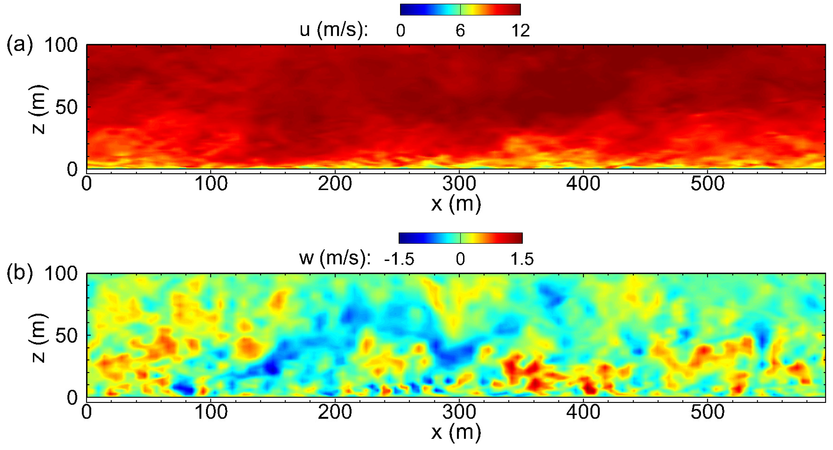
3.2. Instantaneous and Averaged Flow and Aerosol Fields

Figure 3 and Figure 4 illustrate the instantaneous flow fields on the $(x,z)$-plane across the center of the aerosol releasing region for the flat-surface and plane-progressive wave cases, respectively. The LES results showed two main effects induced by the downwind long waves on the wind field. First, the wave-induced form of drag on the wind field caused the wind velocity to reduce (Figure 3a and Figure 4a). Second, the fast surface orbital velocity of the swell waves induced strong disturbance to the wind field, resulting in some strong upwelling events (e.g., at $x=380\mathrm{m}$ in Figure 4b) that may lift the oil aerosol to a considerable elevation.

Figure 5 and Figure 6 show the instantaneous oil aerosol concentrations of the four droplet diameters for the flat-surface and plane-progressive long wave cases, respectively. For both surface conditions, the wind turbulence caused considerable vertical suspension and downwind transport of oil droplets. The droplets with $d=2.5$ μm had negligible slip velocity and were transported like passive tracers. For larger oil droplets, the settling effect caused considerable deposition of oil aerosols back to the water, resulting in lower oil aerosol concentration towards downstream locations. For $d=40$ μm and $d=60$ μm, a large fraction of the oil droplets still remained suspended after being transported through the simulation domain and exited at the outflux boundary at $x=600\mathrm{m}$. The concentration of the suspended oil droplets of $d=100$ μm was much lower than those of other droplet sizes due to the significant settling effect. Note that the upwelling events (with positive vertical velocity fluctuation) in the turbulent boundary layer played a major role in suspending the oil droplets, while the downwelling events (with negative vertical velocity fluctuation) together with the settling effects helped to deposit the oil droplets back to the ocean. The intermittency in the upwelling/downwelling events together with the strong settling effect resulted in the obvious intermittency in the instantaneous distribution of the large oil droplets with $d=100$ μm (Figure 5d and Figure 6d).

It is worth mentioning that for the fast progressive wave case (Figure 6), strong vertical transport of the oil droplets may occur as a result of the upwelling event event caused by the strong wave disturbance (e.g., see the positive vertical velocity fluctuation in Figure 4b and the high oil concentration pocket in Figure 6 at around $x=380\mathrm{m}$), which was capable of lifting even the large $100$ μm droplets to a high elevation (e.g., $40\mathrm{m}$ in the snapshot shown in Figure 6d). A similar upwelling event can also be observed in the flat-surface case, but the magnitude appeared to be relatively weak (e.g., the positive vertical velocity fluctuation in Figure 3b and the high oil concentration in Figure 5 at around $x=340\mathrm{m}$).

The average effects of the plane-progressive wave and slip velocity on the transport of oil aerosol can be obtained by performing the ensemble average of the instantaneous flow field snapshots. In the current analysis, 200 snapshots of the three-dimensional instantaneous flow fields (containing both velocity and oil droplet concentration information) were sampled. These samples were separated by a constant time interval of one wave period (i.e., $T=8.2\mathrm{s}$), which were then averaged to obtain the time-averaged quantity denoted by $\langle ·\rangle$. For an instantaneous physical quantity f, its turbulent fluctuation is defined as $f^{\prime }=f-\langle f\rangle$. Note that for the plane-progressive wave case, because all the instantaneous snapshots were sampled at the same fixed wave phase (see, e.g., Figure 6), the time average $\langle f\rangle$ can also be referred to as the wave phase average [13,39]. Performing the average at the fixed wave phase allowed us to keep the surface wave elevation information in the averaged field, which helped to reveal the effect of waves on the wind turbulence and aerosol transport [12,34].

Using the time average analysis, the enhanced vertical wind motion due to the long plane-progressive waves can be seen clearly from the vertical profiles of the root-mean-square (rms) vertical velocity fluctuation $w_{rms}^{\prime }$ shown in Figure 7. At most of the heights in the simulated domain, the wind turbulence over swell waves exhibited stronger vertical velocity fluctuation, and thus was expected to be able to suspend the oil droplet aerosols to higher elevations under the same pressure gradient forcing condition (i.e., with the same friction velocity of $u_{*}=0.37\mathrm{m}/\mathrm{s}$).

Figure 8 and Figure 9 show the time-averaged oil aerosol concentrations of the four droplet diameters for the flat-surface and plane-progressive wave conditions, respectively. In all cases, the oil aerosol concentration was diluted towards the downstream direction due to the vertical and lateral turbulent dispersions that caused the aerosol plumes to expand (see Figure 2 for example). In addition, the settling motions further reduced the oil droplet concentration, with the effect stronger for larger droplets. For the flat-surface case, the concentrations of the three smaller droplet sizes (i.e., $d=2.5$ μm, $40$ μm and $60$ μm) exhibited a gradual increase of height for the upper edge of the high concentration region caused by the turbulent entrainment at the upper edge of the oil aerosol plume. The upper edge of the average aerosol plume for $d=100$ μm remained almost flat due to the large droplet slip velocity that overcame the upward turbulent entrainment. Differently, Figure 9 showed that the presence of plane-progressive long waves not only enhanced the mean vertical entrainment of oil aerosols (thus resulting in larger vertical extension of the aerosol plumes), but also caused streamwise variations of the averaged concentration field that correlated with the wave phase.

To quantify the downwind development of the oil aerosol plumes over a flat surface and plane-progressive long waves, the center-of-mass height of the plume $z_c$ was calculated based on:

$$z_c\left(x\right)=\frac{{\displaystyle {\int }_{\eta }^{H_0}{\int }_{-L_y/2}^{L_y/2}z\langle C_d\rangle (x,y,z)\mathrm{d}y\mathrm{d}z}}{{\displaystyle {\int }_{\eta }^{H_0}{\int }_{-L_y/2}^{L_y/2}\langle C_d\rangle (x,y,z)\mathrm{d}y\mathrm{d}z}},$$

(27)

where $\langle C_d\rangle$ is the average concentration. Figure 10 shows $z_c\left(x\right)$ for all the simulated cases. For the flat-surface case without the plan-progressive long waves, $z_c$ increased almost linearly with x, with the slope decreasing as the droplet diameter increased. On the other hand, in the plane-progressive wave case, $z_c$ exhibited clearly wave-correlated variation along the x-direction for all four droplet diameters. Similar to the flat-surface case, $z_c$ decreased monotonically as the droplet diameter d increased. Except for $x<90\mathrm{m}$, the value of $z_c$ in the plane-progressive wave case was higher than the corresponding value in the flat-surface case for all four droplet diameters considered in this study.

Moreover, it should be pointed out that the instantaneous oil droplet aerosol concentrations shown in Figure 5 and Figure 6 and the time-averaged oil concentrations shown in Figure 8 and Figure 9 were obtained based on a prescribed continuous source release rate of $1\mathrm{g}/\mathrm{s}$ (see Section 3.1 for the simulation setup). For realistic oil spill accidents, the surface oil slicks may release droplet aerosols in an intermittent manner with a release rate different from the one used in this study depending on the wind condition and sea state. Caution should be given when estimating the air quality based on the idealized simulation setup used in this study. Nevertheless, the statistical results reported here still provide some useful insights for understanding the dispersion of the oil droplet aerosols in the MABL. At the very least, one may be able to estimate the order of magnitude of the oil droplet concentration by rescaling the results reported in Figure 8 and Figure 9 based on the actual aerosol release rate under similar wind and sea conditions.

4. Conclusions

In this study, a hybrid LES model was developed and applied to simulate the oil droplet aerosol transport in the MABL. The model featured a wave surface-fitted grid to help capture the detailed flow physics in the wind adjacent to the wave surface. Aerosol transport over pure wind-sea was modeled by simplifying the sea surface as a flat boundary, on which the effect of unresolved short waves was parameterized as the surface roughness. In another case, the effect of ocean swell waves was modeled by directly imposing the wave elevation and surface orbital velocities as the bottom boundary conditions of the LES. For oil droplets released from a source region on the water surface, the simulation results showed considerable suspension and downwind transport of aerosol by the turbulence in the MABL. When plane-progressive long waves (swells) were present, their highly-organized wave motions induced strong distortion to the lower portion of the MABL and enhanced the vertical turbulence fluctuation, resulting in enhanced aerosol suspension and wave-phase-correlated streamwise variations.

References

1. Veron, F. Ocean spray. Annu. Rev. Fluid Mech. 2015, 47, 507–538. [Google Scholar] [CrossRef]
2. Zhuang, Y.; Lozowski, E.P.; Wilson, J.D.; Bird, G. Sea spray dispersion over the ocean surface: A numerical simulation. J. Geophys. Res. 1993, 98, 16547–16553. [Google Scholar] [CrossRef]
3. Mestayer, P.G.; van Eijk, A.M.J.; de Leeuw, G.; Tranchant, B. Numerical simulation of the dynamics of sea spray over the waves. J. Geophys. Res. 1996, 101, 20771–20797. [Google Scholar] [CrossRef]
4. Andreas, E.L.; Persson, P.O.G.; Hare, J.E. A bulk turbulent air–sea flux algorithm for high-wind, spray conditions. J. Phys. Oceanogr. 2008, 38, 1581–1596. [Google Scholar] [CrossRef]
5. Kudryavtsev, V.N.; Makin, V.K. Impact of ocean spray on the dynamics of the marine atmospheric boundary layer. Bound. Layer Meteorol. 2011, 140, 383–410. [Google Scholar] [CrossRef]
6. Tang, S.; Yang, Z.; Liu, C.; Dong, Y.; Shen, L. Numerical study on the generation and transport of spume droplets in wind over breaking waves. Atmosphere 2017, 8, 248. [Google Scholar] [CrossRef]
7. Yang, Z.; Deng, B.; Shen, L. Direct numerical simulation of wind turbulence over breaking waves. J. Fluid Mech. 2018, 850, 120–155. [Google Scholar] [CrossRef]
8. Sullivan, P.P.; Edson, J.B.; Hristov, T.; McWilliams, J.C. Large-eddy simulations and observations of atmospheric marine boundary layers above nonequilibrium surface waves. J. Atmos. Sci. 2008, 65, 1225–1245. [Google Scholar] [CrossRef]
9. Sullivan, P.P.; McWilliams, J.C.; Patton, E.G. Large-eddy simulation of marine atmospheric boundary layers above a spectrum of moving waves. J. Atmos. Sci. 2014, 71, 4001–4027. [Google Scholar] [CrossRef]
10. Yang, D.; Meneveau, C.; Shen, L. Dynamic modelling of sea surface roughness for large-eddy simulation of wind over ocean wavefield. J. Fluid Mech. 2013, 726, 62–99. [Google Scholar] [CrossRef]
11. Yang, D.; Meneveau, C.; Shen, L. Large-eddy simulation of offshore wind farm. Phys. Fluids 2014, 26, 025101. [Google Scholar] [CrossRef]
12. Yang, D.; Meneveau, C.; Shen, L. Effect of downwind swells on offshore wind energy harvesting—A large-eddy simulation study. Renew. Energy 2014, 70, 11–23. [Google Scholar] [CrossRef]
13. Hara, T.; Sullivan, P.P. Wave boundary layer turbulence over surface waves in a strongly forced condition. J. Phys. Oceanogr. 2015, 45, 868–883. [Google Scholar] [CrossRef]
14. McWilliams, J.C.; Sullivan, P.P. Vertical mixing by Langmuir circulation. Spill Sci. Technol. Bull. 2000, 6, 225–237. [Google Scholar] [CrossRef]
15. Skyllingstad, E.D. Scales of Langmuir circulation generated using a large-eddy simulation model. Spill Sci. Technol. Bull. 2000, 6, 239–246. [Google Scholar] [CrossRef]
16. Noh, Y.; Kang, I.S.; Herold, M.; Raasch, S. Large eddy simulation of particle settling in the ocean mixed layer. Phys. Fluids 2006, 18, 085109. [Google Scholar] [CrossRef]
17. Liang, J.-H.; McWilliams, J.C.; Sullivan, P.P.; Baschek, B. Large eddy simulation of the bubbly ocean: New insights on subsurface bubble distribution and bubble-mediated gas transfer. J. Geophys. Res. 2012, 117, C04002. [Google Scholar] [CrossRef]
18. Kukulka, T.; Brunner, K. Passive buoyant tracers in the ocean surface boundary layer: 1. Influence of equilibrium wind-waves on vertical distributions. J. Geophys. Res. Ocean. 2014, 120, 3837–3858. [Google Scholar] [CrossRef]
19. Yang, D.; Chamecki, M.; Meneveau, C. Inhibition of oil plume dilution due to Langmuir ocean circulation. Geophys. Res. Lett. 2014, 41, 1632–1638. [Google Scholar] [CrossRef]
20. Yang, D.; Chen, B.; Chamecki, M.; Meneveau, C. Oil plumes and dispersion in Langmuir, upper-ocean turbulence: Large-eddy simulations and K-profile parameterization. J. Geophys. Res. Ocean. 2015, 120, 4729–4759. [Google Scholar] [CrossRef]
21. Chen, B.; Yang, D.; Meneveau, C.; Chamecki, M. Effects of swell on transport and dispersion of oil plumes within the ocean mixed layer. J. Geophys. Res. Ocean. 2016, 121, 3564–3578. [Google Scholar] [CrossRef] [Green Version]
22. Chor, T.; Yang, D.; Meneveau, C.; Chamecki, M. Preferential concentration of noninertial buoyant particles in the ocean mixed layer under free convection. Phys. Rev. Fluids 2018, 3, 064501. [Google Scholar] [CrossRef]
23. Calaf, M.; Meneveau, C.; Meyers, J. Large eddy simulation study of fully developed wind-turbine array boundary layers. Phys. Fluids 2010, 22, 015110. [Google Scholar] [CrossRef] [Green Version]
24. Chamecki, M.; Meneveau, C.; Parlange, M. Large eddy simulation of pollen transport in the atmospheric boundary layer. J. Aerosol Sci. 2009, 40, 241–255. [Google Scholar] [CrossRef]
25. Smagorinsky, J. General circulation experiments with the primitive equations. I. The basic experiment. Mon. Weather Rev. 1963, 91, 99–164. [Google Scholar] [CrossRef]
26. Lilly, D.K. The representation of small-scale turbulence in numerical simulation experiments. In Proceedings of the IBM Scientific Computing Symposium on Environmental Science, Yorktown Heights, NY, USA, 14–16 November 1966; Goldstein, H.H., Ed.; pp. 195–210. [Google Scholar]
27. Bou-Zeid, E.; Meneveau, C.; Parlange, M. A scale-dependent Lagrangian dynamic model for large eddy simulation of complex turbulent flows. Phys. Fluids 2005, 17, 025105. [Google Scholar] [CrossRef] [Green Version]
28. Kumar, V.; Svensson, G.; Holtslag, A.A.; Meneveau, C.; Parlange, M.B. Impact of surface flux formulations and geostrophic forcing on large-eddy simulations of diurnal atmospheric boundary layer flow. J. Appl. Meteorol. Climatol. 2010, 49, 1496–1516. [Google Scholar] [CrossRef]
29. Afshar-Mohajer, N.; Li, C.; Rule, A.M.; Katz, J.; Koehler, K. A laboratory study of particulate and gaseous emissions from crude oil and crude oil-dispersant contaminated seawater due to breaking waves. Atmos. Environ. 2018, 179, 177–186. [Google Scholar] [CrossRef]
30. Sampath, K.; Afshar-Mohajer, N.; Chandrala, L.D.; Heo, W.S.; Gilbert, J.; Austin, D.; Koehler, K.; Katz, J. Aerosolization of crude oil?dispersant slicks due to bubble bursting. J. Geophys. Res. Atmos. 2019, 124, 5555–5578. [Google Scholar] [CrossRef]
31. Clift, R.; Gauvin, W.H. The motion of particles in turbulent gas streams. Proc. Chemeca 1970, 1, 14–28. [Google Scholar]
32. Yang, D.; Chen, B.; Socolofsky, S.A.; Chamecki, M.; Meneveau, C. Large-eddy simulation and parameterization of buoyant plume dynamics in stratified flow. J. Fluid Mech. 2016, 794, 798–833. [Google Scholar] [CrossRef]
33. Wan, F.; Porté-Agel, F.; Stoll, R. Evaluation of dynamic subgrid-scale models in large-eddy simulations of neutral turbulent flow over a two-dimensional sinusoidal hill. Atmos. Environ. 2007, 41, 2719–2728. [Google Scholar] [CrossRef]
34. Yang, D.; Shen, L. Direct-simulation-based study of turbulent flow over various waving boundaries. J. Fluid Mech. 2010, 650, 131–180. [Google Scholar] [CrossRef] [Green Version]
35. Yang, D.; Shen, L. Simulation of viscous flows with undulatory boundaries. Part I. Basic solver. J. Comput. Phys. 2011, 230, 5488–5509. [Google Scholar] [CrossRef]
36. Gaskell, P.H.; Lau, A.K.C. Curvature-compensated convective transport: SMART, a new boundedness-preserving transport algorithm. Int. J. Numer. Methods Fluids 1988, 8, 617–641. [Google Scholar] [CrossRef]
37. Chamecki, M.; Meneveau, C.; Parlange, M.B. A hybrid spectral/finite-volume algorithm for large-eddy simulation of scalars in the atmospheric boundary layer. Bound. Layer Meteorol. 2008, 128, 473–484. [Google Scholar] [CrossRef]
38. Belcher, S.E.; Hunt, J.C.R. Turbulent flow over hills and waves. Annu. Rev. Fluid Mech. 1998, 30, 507–538. [Google Scholar] [CrossRef]
39. Sullivan, P.P.; McWilliams, J.C.; Moeng, C.-H. Simulation of turbulent flow over idealized water waves. J. Fluid Mech. 2000, 404, 47–85. [Google Scholar] [CrossRef] [Green Version]
Figure 1. Illustration of boundary-fitted grid and coordinate transformation: (a) ( x , z ) -plane in the physical space; (b) ( ξ , ζ ) -plane in the computational space. For illustration purposes, the grid lines shown in (a,b) are plotted for every two actual grids used in the simulation.
Atmosphere 10 00459 g001
Figure 2. Illustration of three-dimensional instantaneous flow and aerosol fields for wind over swell waves. Contours of the instantaneous streamwise velocity u are shown on the two vertical planes. The oil aerosol field for d = 2.5 μm is visualized by the isosurface of oil droplet concentration C d = 1 × 10 4 g / m 3 .
Atmosphere 10 00459 g002
Figure 3. Instantaneous flow field on the ( x , z ) -plane across the center of the surface release region for the flat-surface case: (a) streamwise velocity u; (b) vertical velocity w.
Atmosphere 10 00459 g003
Figure 4. Instantaneous flow field on the ( x , z ) -plane across the center of the surface release region for the 100 m plane-progressive wave case: (a) streamwise velocity u; (b) vertical velocity w.
Atmosphere 10 00459 g004
Figure 5. Instantaneous oil aerosol concentrations on the ( x , z ) -plane across the center of the surface release region for the flat-surface case: (a) d = 2.5 μm; (b) d = 40 μm; (c) d = 60 μm; (d) d = 100 μm.
Atmosphere 10 00459 g005
Figure 6. Instantaneous oil aerosol concentrations on the ( x , z ) -plane across the center of the surface release region for the swell wave case: (a) d = 2.5 μm; (b) d = 40 μm; (c) d = 60 μm; (d) d = 100 μm.
Atmosphere 10 00459 g006
Figure 7. Vertical profiles of vertical velocity fluctuation rms w r m s . The solid line is for the plane-progressive wave case, and the dashed line is for the flat-surface case.
Atmosphere 10 00459 g007
Figure 8. Time-averaged oil aerosol concentrations on the ( x , z ) -plane across the center of the surface release region for the flat-surface case: (a) d = 2.5 μm; (b) d = 40 μm; (c) d = 60 μm; (d) d = 100 μm.
Atmosphere 10 00459 g008
Figure 9. Time-averaged oil aerosol concentrations on the ( x , z ) -plane across the center of the surface release region for the plane-progressive wave case: (a) d = 2.5 μm; (b) d = 40 μm; (c) d = 60 μm; (d) d = 100 μm.
Atmosphere 10 00459 g009
Figure 10. Center-of-mass height z c of oil aerosols as a function of the streamwise location. The solid lines are for the plane-progressive wave case, and the dashed lines are for the flat-surface benchmark cases.
Atmosphere 10 00459 g010