Multi-Channel Regression Inversion Method for Passive Remote Sensing of Ice Water Path in the Terahertz Band

Abstract

Retrieval of ice cloud properties using passive terahertz wave radiometer from space has gained increasing attention currently. A multi-channel regression inversion method for passive remote sensing of ice water path (IWP) in the terahertz band is presented. The characteristics of the upward terahertz radiation in the clear-sky and cloudy-sky are first analyzed using the Atmospheric Radiative Transfer Simulator (ARTS). Nine representative center frequencies with different offsets are selected to study the changes of terahertz radiation caused by microphysical parameters of ice clouds. Then, multiple linear regression method is applied to the inversion of IWP. Combinations of different channels are selected for regression to eliminate the influence of other factors (i.e., particle size and cloud height). The optimal fitting equation are obtained by the stepwise regression method using two oxygen absorption channels (118.75 ± 1.1 GHz, 118.75 ± 3.0 GHz), two water vapor absorption channels (183.31 ± 1.0 GHz, 183.31 ± 7.0 GHz), and two window channels (243.20 ± 2.5 GHz, 874.4 ± 6.0 GHz). Finally, the errors of the proposed inversion method are evaluated. The simulation results show that the absolute errors of this method for the low IWP cases are below 7 g/m², and the relative errors for the high IWP cases are generally ranging from 10 to 30%, indicating that the multi-channel regression inversion method can achieve satisfactory accuracy.

1. Introduction

Ice clouds, often occurring in the upper troposphere and the lower stratosphere, play a significant role in the balance of the energy budget since they can both reflect the incoming solar radiation and trap thermal infrared emission from the lower atmosphere and the surface. The physical properties of ice clouds have become important parameters in the weather and climate numerical models, especially the ice water path (IWP), which is an indispensable parameter used to describe the column-integrated bulk mass of ice inside the clouds [1,2]. However, measuring the IWP continues to remain a challenging task nowadays. There are limited numbers of high-quality global observations, and we lack the understanding of the microphysical and optical properties of ice clouds, and substantial uncertainties remain in the representation of ice clouds in radiative transfer models, which further influences the accuracy of weather and climate modelling. Therefore, there is an urgent need to obtain the properties of ice clouds precisely on a global scale.

Existing methods to estimate the ice water path can be divided into three categories: passive sensors within the infrared and visible ranges of the electromagnetic spectrum, active sensors such as radar or LiDAR, or combinations of different sensors [3]. For passive remote sensing in the infrared and optical band, because of the high absorbing properties of ice clouds in this band, the penetrability of the electromagnetic wave is very low when cloud is thick. Therefore these sensors can only sense the thin ice clouds or the upper layer of thick ice clouds [4]. Active remote sensing methods are more suitable for the inversion of the vertical structure of ice clouds; however, they only sample the atmosphere just below the satellite, so their horizontal coverage is limited compared with passive remote sensing methods [5]. For joint observation methods, since they combine the advantages of different sensors, a higher estimation accuracy can be achieved, where Holl et al. have showed that the remote sensing method that combines the radar and LiDAR can achieve higher estimation accuracy than any passive sensors. However, it should be noted that the wavelengths applied by both the optical and microwave instruments to remote sense the ice clouds are much smaller or larger than the actual size of the ice crystals, so the signals received are not very sensitive to the cloud particles. To solve this problem, many researchers are resort to use the terahertz wave, which is located between infrared and microwave band. Compared with the traditional methods, remote sensing by terahertz wave have several advantages: (1) since its wavelength is similar to the size of ice cloud particles, it is more sensitive to ice crystals than visible, infrared and microwave; (2) there is a good penetrability of the cloud in the terahertz band, so it can sense the whole column of the cloud with a large field of view.

Considering its huge potential in remote sensing of ice clouds, the United States, Europe and other countries have successively proposed several plans to develop spaceborne terahertz, which includes SIRICE, GOMAS, CIWSIR, CloudIce, IceCube, ICI and so on. With the maturity of related instruments, some proven airborne terahertz ice cloud detectors have been developed, such as CoSSIR [6], ISMAR [7] and so on. The inversion algorithm has also been studied, notably include the Bayesian Monte Carlo Integration (BMCI) and the Neural Network (NN), and these inversion methods need to generate a pre-calculated retrieval database, which contains the full range of relevant atmospheric/cloud situations and the brightness temperatures simulated by radiative transfer models. Evans et al. first proposed the method of BMCI and tested its performance using simulated brightness temperatures [8], then applied this method to retrieve the IWP and particle size form the observations in the CRYSTAL-FACE campaigns [9]. The priori database was built using randomly generated profiles and microphysics, with the statistics taken from radiosondes and aircraft campaigns. Jiménez et al. first proposed the method of NN to retrieve ice cloud parameters [10], and they tested the retrieval accuracy of IWP, particle size and cloud height using two databases, Colorado training dataset and Chalmers training dataset [11]. Colorado training dataset used the statistics obtained from soundings and radars from the Atmospheric Radiation Measurement (ARM) programme. Chalmers training dataset used statistics from the European Center for Medium-range Weather Forecasts (ECMWF), CloudNET ground-based radars, and the in situ measurements as in Rydberg et al. [12]. Brath et al. applied the NN method to retrieve the snow ice water path, liquid water path, and integrated water vapor from the observations in the airborne radiometers (ISMAR and MARSS). The atmospheric profiles in the training database were taken from the Icosahedral Nonhydrostatic (ICON) numerical weather prediction model [3]. It can be seen that the two inversion methods are based on a perfect and practical retrieval database, and the inversion accuracy depends heavily on the information amount of it. Moreover, the database is typically developed for one geographic region and season.

China is also studying passive spaceborne terahertz wave instruments at present, and research on inversion methods of ice clouds by terahertz has also made progress [13,14,15]. This paper first uses the Atmospheric Radiative Transfer Simulator (ARTS) to analyze the sensitivity of typical channels to ice cloud microphysical parameters in terahertz band, and reveals the different responses of different channels. When there is a lack of a priori physical properties of the ice clouds and the retrieval database cannot be constructed, based on the theoretical results of simulation, we attempt to provide a new approach to retrieve IWP at a low cost, which is faster and simpler. The method of multi-channel linear regression is adopted to eliminate the influence of other correlative parameters (i.e., particle size and cloud height), so as to realize the inversion of IWP directly by passive remote sensing in the terahertz band.

2. Methods of Simulation

2.1. Forward Model and Simulator

The atmospheric transmission of terahertz radiation includes atmospheric emission, attenuation and other basic processes. Atmospheric attenuation is mainly caused by absorption of gas molecules and scattering of particles. Scattering is mainly due to aerosols and condensations of water vapor, such as clouds, rain and snow. Terahertz wavelength is similar to that of the ice cloud particle, so the scattering effect is strong. The upward thermal radiation generated by the surface and the lower layer of the warmer atmosphere is reduced by the scattering effect of the ice cloud particles. Additionally, the decreased brightness temperature received by the radiometer is directly related to the parameters of ice clouds, so a specific relationship between the brightness temperature attenuation and the ice water path can be established.

ARTS (the Atmospheric Radiative Transfer Simulator) is a highly modular, expandable and universally applicable software, which can be used to simulate and calculate the atmospheric radiative transfer from microwave to thermal infrared [16]. The atmospheric profiles of temperature, relative humidity, pressure and trace gas composition as inputs to simulator are from the FASCOD standard database [17], and the spectrum parameters of molecular absorption are from the HITRAN2012 database extracted by the line-by-line integration [18]. Scattering parameters of ice cloud particles are derived from the single scattering property database of non-spherical particles calculated by Discrete Dipole Approximation (DDA) algorithm and the single scattering property of spherical particles calculated by Mie theory [19]. Subsequently, the method of Discrete Ordinate ITerative (DOIT) in ARTS is adopted to deal with the scattering simulation of cloud particles.

2.2. Basic Microphysical Parameters

The single scattering characteristics of ice cloud particles are related to their microphysical parameters, mainly including particle shape and particle size. The shape of the particles depends on temperature, relative humidity and physical process of formation. The shapes of ice cloud particles vary greatly from area to area, including aggregate, solid or hollow column, plate, bullet rosette, sphere and so on. Methods for describing single non-spherical particle size of ice cloud mainly include maximum size, equal mass spherical particle size and equal volume spherical particle size. In this paper, the effective particle size of non-spherical particles is calculated using the fitting relation between the equal volume spherical particle diameter and maximum size based on a large amount of observation data established by Yang et al. [20].

The actual particle swarm of ice cloud contains many particles of different sizes, ranging from a few micrometers to thousands of micrometers. The size distribution function $n(r)$ can be used to represent the number of particles per unit volume per unit radius interval. In the radiative transfer model, the most commonly used is Gamma distribution [21], which is in the form of:

$$n(r)=a{r}^{\alpha }\exp (br)$$

(1)

where, dimensionless parameter $\alpha$ represents the width of shape distribution, generally set as 1, and a and b are concentration parameters and scale parameters respectively, which are related to ice water content (IWC) and effective particle radius ($R_{eff}$) as follows:

$$a=\frac{IWC}{4/3\pi \rho b^{-(\alpha +4)}\Gamma [\alpha +4]}$$

(2)

$$b=\frac{\alpha +3}{R_{eff}}$$

(3)

where, ρ is the density of the scattering medium, for ice clouds, ρ corresponds to the bulk density of ice, which is approximately 917 kg/m³. Γ is the Gamma function, ice water content (IWC) is the mass of ice cloud contained in the cloud per unit volume (g/m³), and ice water path (IWP) is defined as the integral of ice water content between thickness of the ice cloud (g/m²).

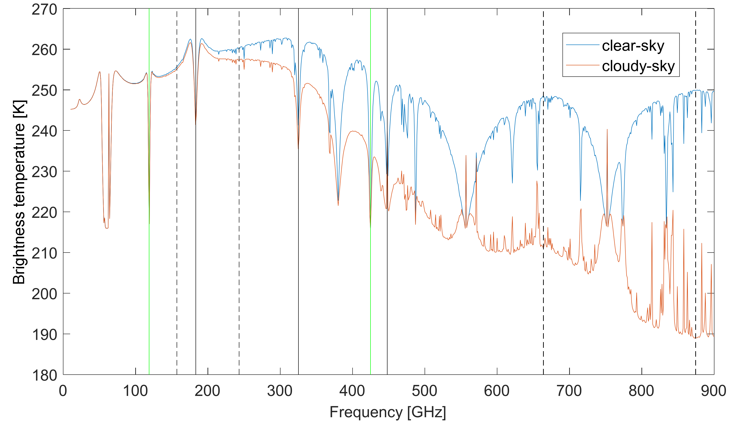
2.3. Selection of Channels

Selecting the appropriate channels in terahertz wave is the first step of the detection technology of ice clouds. The actual radiometer’s channel is a passband with a certain width. For the same central frequency, there are usually several different offsets. Considering the current research status, such as Compact Scanning Submillimeter-wave Imaging Radiometer (CoSSIR), International Submillimeter Airborne Radiometer (ISMAR), Ice Cloud Imager (ICI) and so on; information of the representative channels is shown in

Table 1. Information of representative channels.

Center Frequency (GHz)	Frequency Offset (GHz)	Channel Characteristics	Channel Number
118.75	±1.1, ±1.5, ±2.1, ±3.0, ±5.0	oxygen	(1.1), (1.2), (1.3), (1.4), (1.5)
157.05	±2.6	window	(2)
183.31	±1.0, ±3.0, ±7.0	water vapor	(3.1), (3.2), (3.3)
243.20	±2.5	window	(4)
325.15	±1.5, ±3.5, ±9.5	water vapor	(5.1), (5.2), (5.3)
424.70	±1.0, ±1.5, ±4.0	oxygen	(6.1), (6.2), (6.3)
448.0	±1.4, ±3.0, ±7.2	water vapor	(7.1), (7.2), (7.3)
664.0	±4.2	window	(8)
874.4	±6.0	window	(9)

.

Figure 1 shows the brightness temperature of 10–900 GHz detected at the top of the atmosphere using the ARTS simulation of mid-latitude winter clear-sky and ice cloudy-sky. The ice cloud is assumed to be a homogenous cloud with a height of 8–10 km and an ice water path of 80 g/m². The cloud contains spherical ice crystal particles with an effective particle diameter of 200 μm. It can be seen that the ice cloud has almost no influence on the upward radiation of frequencies below 100 GHz, but has a greater impact above 100 GHz, which also indicates that the terahertz wave can be more effectively used for the detection of ice clouds. In addition, center frequencies of nine representative channels are marked in the figure, the solid black lines are the water vapor absorption channels, the solid green lines are the oxygen absorption channels, and the dashed lines are the window channels. It can be seen that the value of brightness temperature of the clear sky in the absorption channel is significantly smaller than that of the surrounding frequencies, indicating that the terahertz wave is strongly attenuated in the process of upward transmission. Additionally, there is an obvious difference in the bright temperature between the clear-sky and the ice cloudy-sky in the frequencies around the absorption channel.

Selecting the absorption line as the center frequency, on the one hand, can minimize the influence of the surface, the lower atmosphere and other absorption gases on the brightness temperature. On the other hand, by setting the offsets, the information of ice clouds at different heights can be obtained at a small cost. In order to minimize the effect of ozone on the received radiation, the selection of channels should avoid the ozone absorption line, but for 183 GHz, this effect cannot be completely ignored [22]. Due to the weak ability of penetration, the high-frequency channels are sensitive to high clouds, while the low-frequency channels can detect low ice clouds. For channels with different offsets of the same center frequency, the channels with smaller frequency offsets are more sensitive to high clouds because they are closer to the absorption line and have higher opacity. At the same time, the difference between the clear-sky and the ice cloudy-sky in the atmospheric window region is significant, so the window channels can be used to obtain the information of ice clouds different from the absorption line.

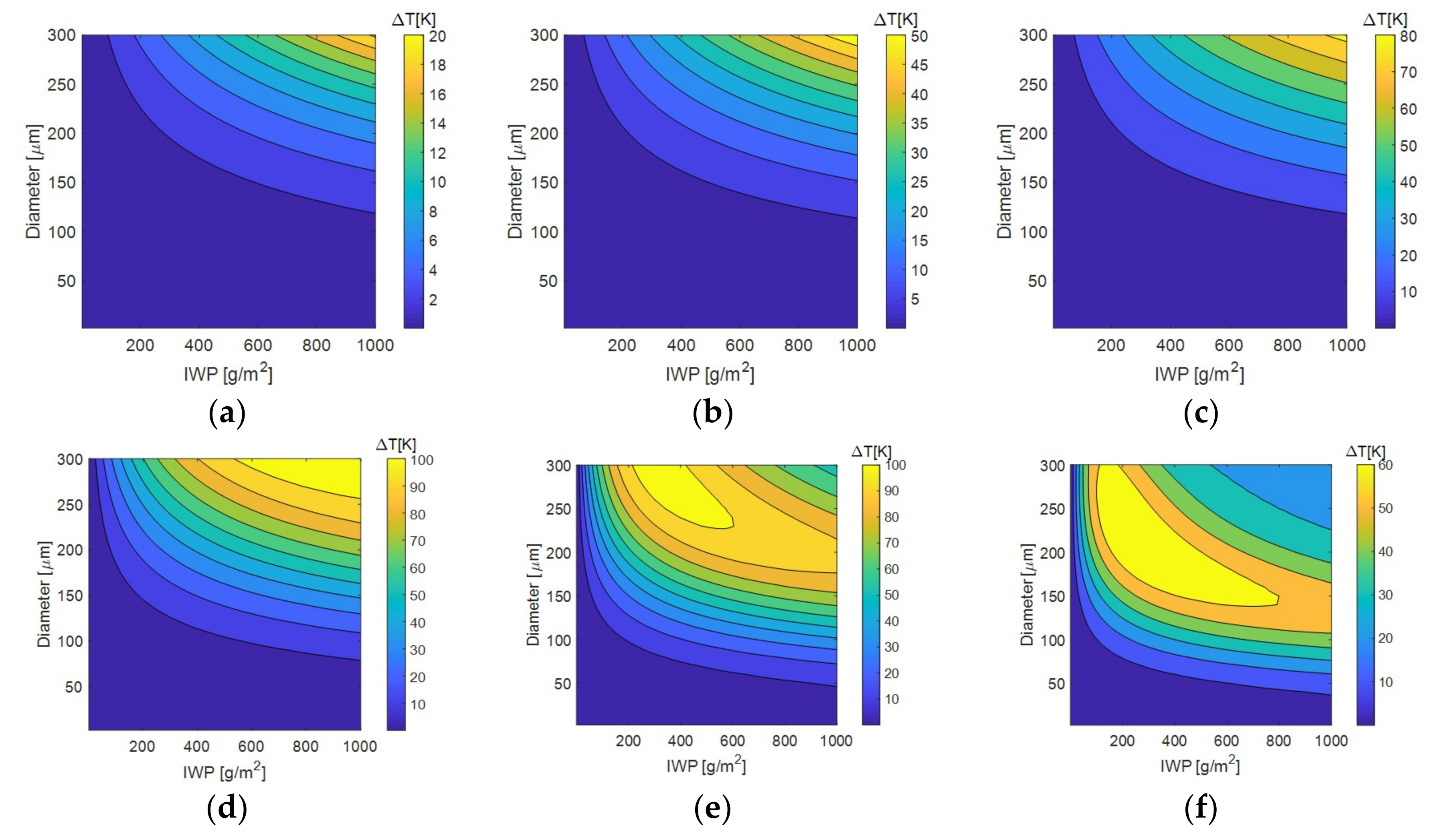
3. Influence of Ice Cloud on Terahertz Radiation

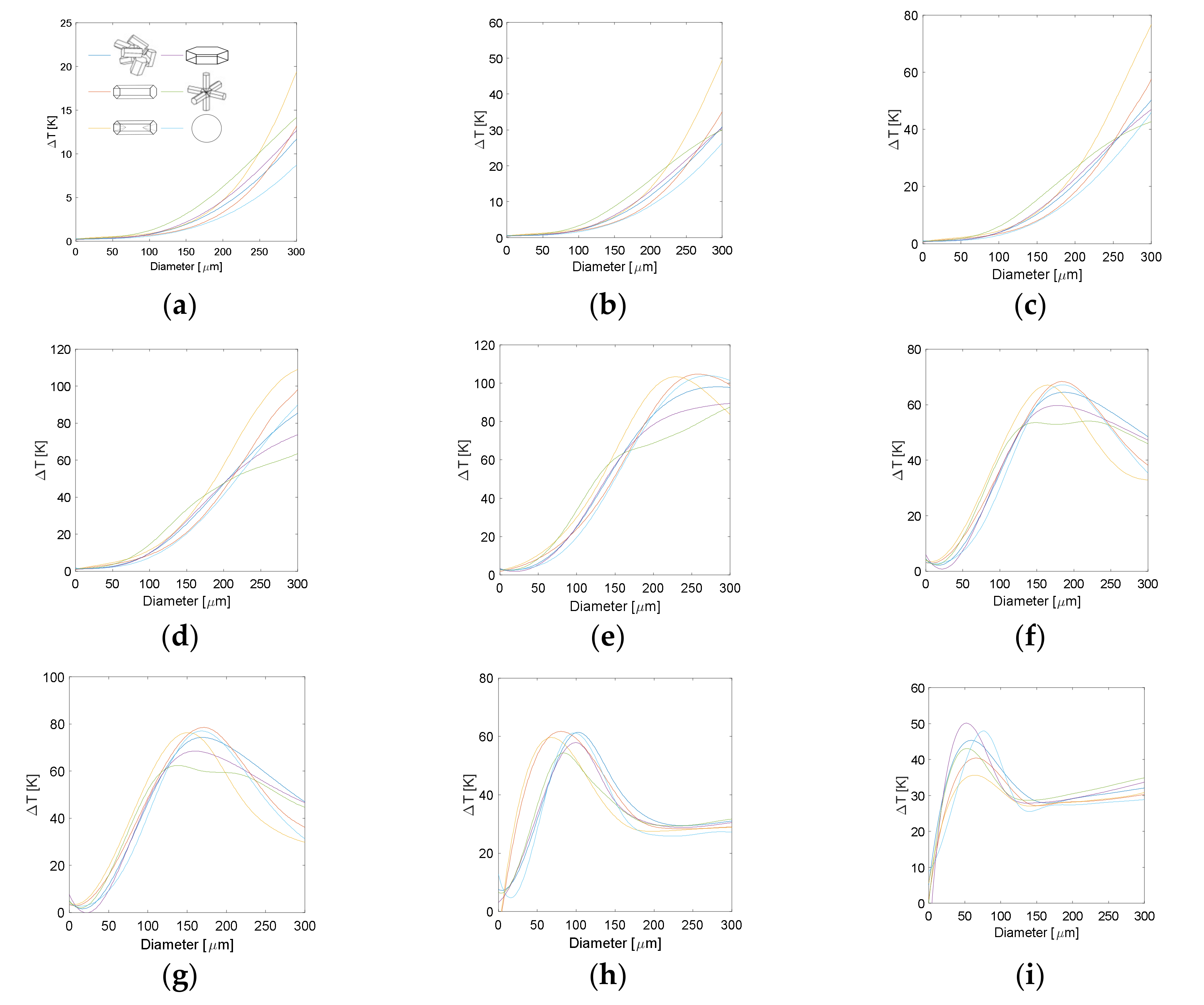
3.1. Effect of Particle Shape

Figure 2 shows the variation of the brightness temperature difference (ΔT) detected at the top of the atmosphere with different effective particle sizes for different particle shapes when one offset of the nine center frequencies is chosen. ΔT is defined as the simulated brightness temperature value in the clear-sky minus that in the ice cloudy-sky. The ice cloud is assumed to be homogeneous with a height of 8–9 km and an ice water path of 400 g/m². It can be seen that the shape of the ice cloud particles affects its scattering characteristics, and the influence on the terahertz radiation at the top of the atmosphere is irregular. However, this effect is much smaller than the effect of particle size. When different particle shapes are used, the overall trend of the ΔT during nadir observations with the effective particle diameter is consistent. Because when the ice crystals in the cloud have many different mixed shapes and orientations, the total intensity received is less affected by the shape of the particles, and their asymmetric scattering properties of individual ice crystals are effectively averaged [23,24]. Moreover, ice particles are typically smaller than snow particles and hence are less effective scatterers, so the choice of particle shape is less important for cloud ice than for precipitation [21]. Therefore, it is preliminarily assumed that the shape of the ice cloud particles is spherical in the simulation, and the Mie scattering theory can be used to simplify the calculation.

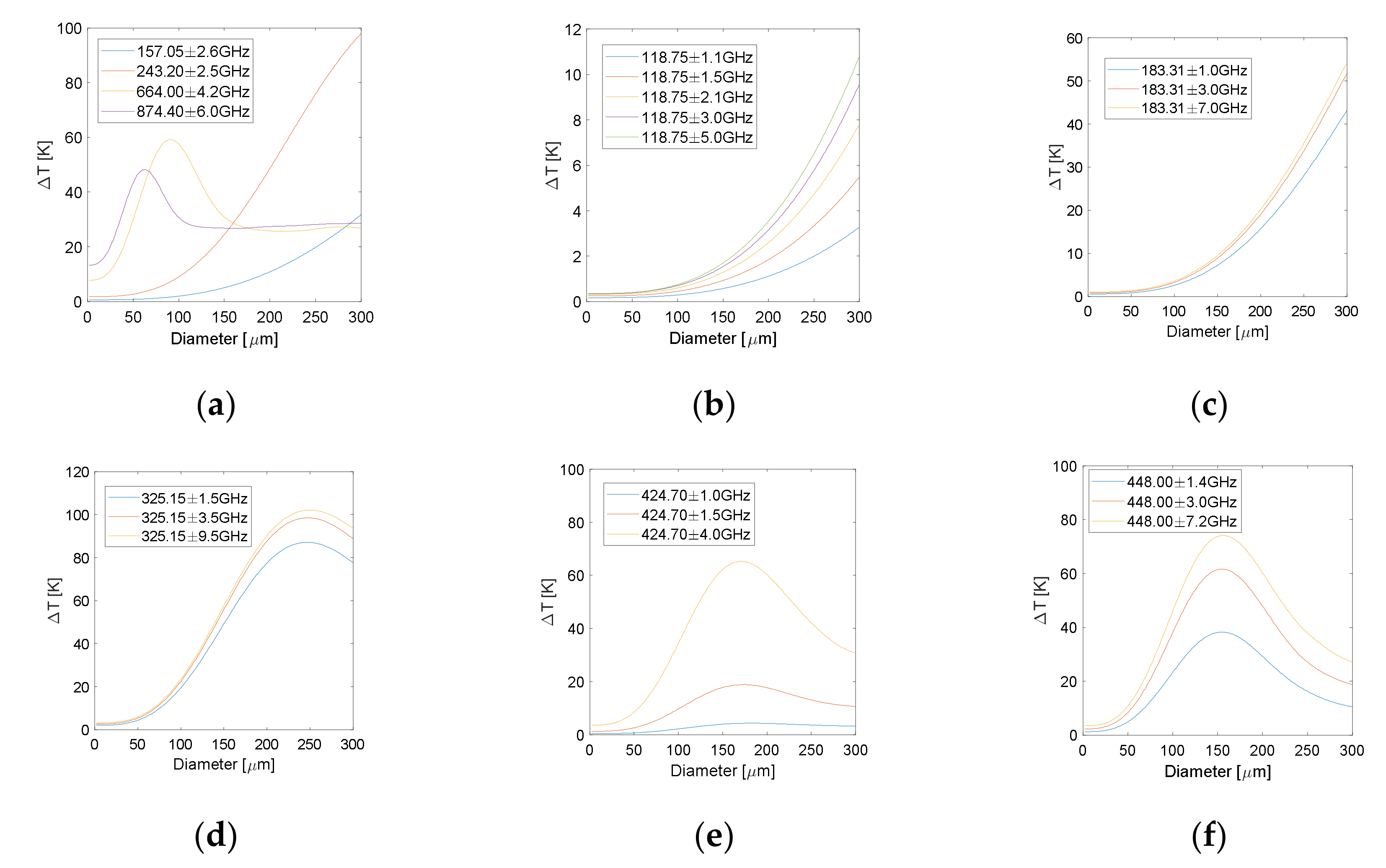
3.2. Effect of Effective Particle Size

Figure 3 shows the variation of the ΔT detected at the top of the atmosphere with different effective particle diameters in all selected channels. The ice cloud is assumed to be a homogeneous cloud with a height of 8–9 km and an ice water path of 500 g/m². It can be seen that the sensitivities of different frequencies to the effective particle size is quite different. The ΔT of low-frequency channels such as 118.75 GHz, 157.05 GHz, 183.31 GHz and 243.20 GHz are monotonically increasing as the effective particle diameter becomes larger. Therefore, ΔT of low frequency is large for big particles, and it is easy to retrieve big particles through the brightness temperature detected by low-frequency channels. The ΔT of high-frequency channels first increase rapidly and then decrease, and the higher the frequency, the maximum ΔT occurs at the smaller effective particle diameter. So ΔT of high frequency is large for small particles, moreover, the ΔT has a large slope with small particle size, it is easy to distinguish small particles through high-frequency channels. This indicates that the interaction between high frequencies and small particles is stronger, while the interaction between low frequencies and big particles is stronger. At the same time, for channels with different offsets of the same center frequency, the larger the frequency offset is, the larger the ΔT is, especially for the oxygen absorption channel of 424.70 GHz, showing that the channel with larger frequency deviation is far away from the absorption line and has a higher transparency, so it can detect lower ice clouds, and the channel with smaller frequency deviation is more sensitive to high thin clouds.

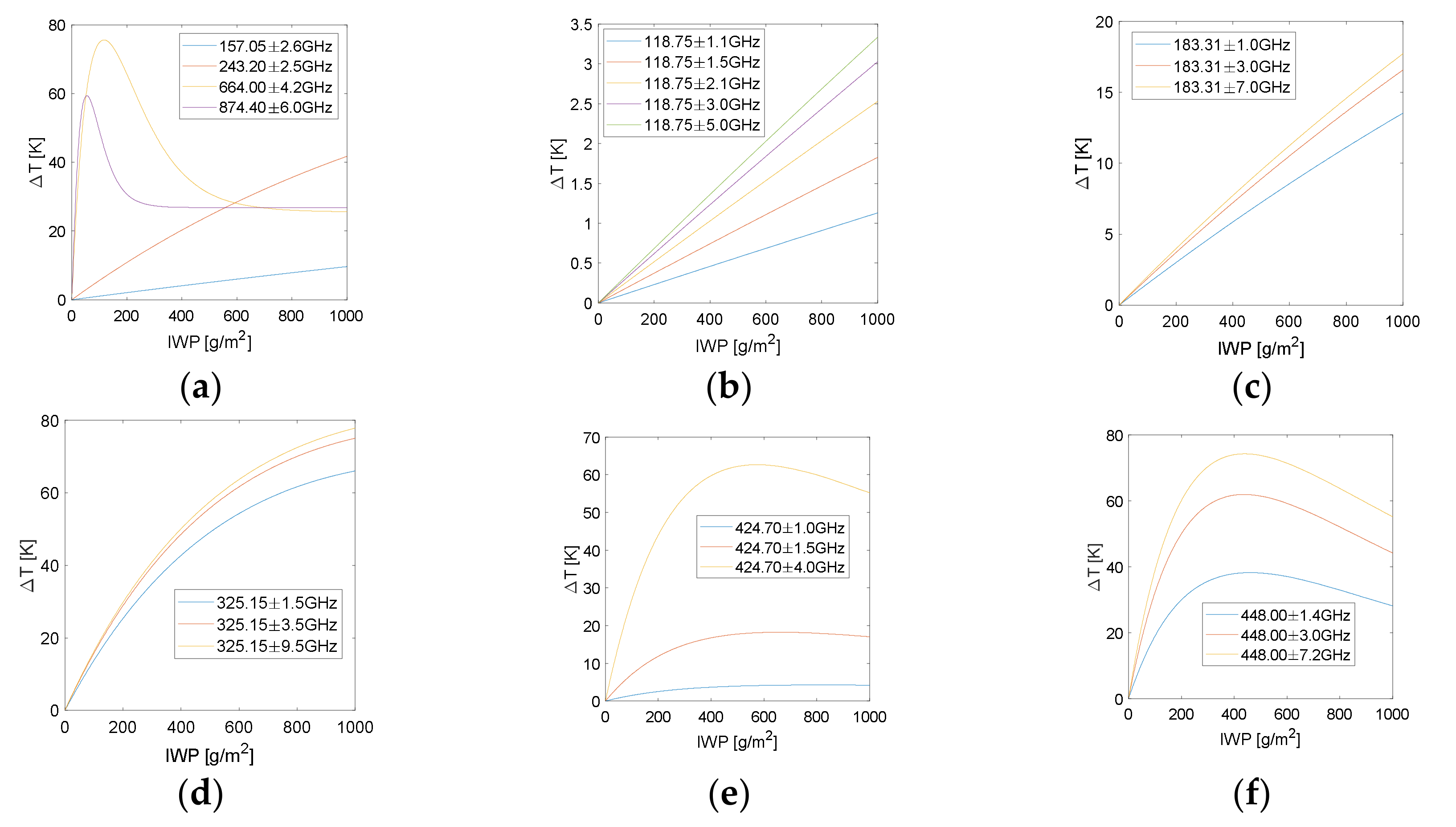
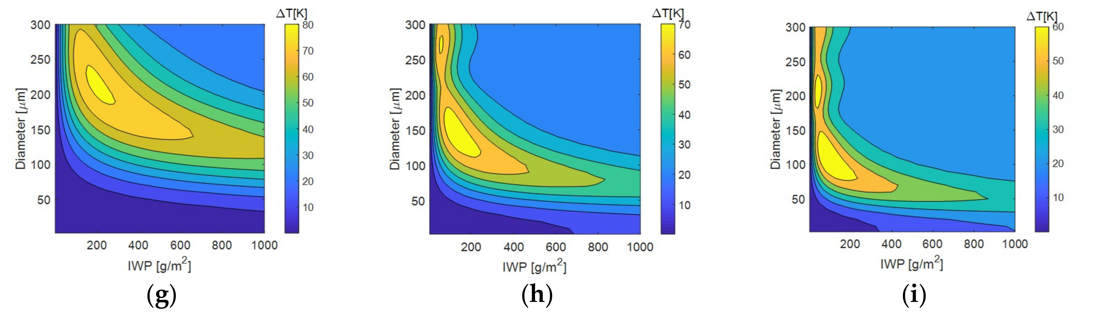
3.3. Effect of Ice Water Path

Figure 4 shows the variation of the ΔT detected at the top of the atmosphere with different ice water paths in all selected channels. The ice cloud is assumed to be a homogeneous cloud with a height of 8–9 km and an effective particle diameter of 150 μm. Similar to the effect of effective particle size on the terahertz radiation, The ΔT of high-frequency channels first increase rapidly and then decrease, and the higher the frequency, the maximum ΔT occurs at the smaller value of ice water path. Therefore, the high frequency is sensitive to the low ice water path and can be used to detect high thin ice clouds. The ΔT of low-frequency channel increases monotonously and is approximately proportional to the ice water path. As the frequency increases, the ΔT starts to saturate at a point of ice water path, and the higher the frequency, the earlier the saturation begins. Meanwhile, for channels with different offsets of the same center frequency, the larger the frequency offset is, the larger the ΔT is. This also shows that the channel with larger frequency offset has higher transparency, the lower ice clouds can be detected, and the channel with smaller frequency offset is more suitable to detect high clouds.

4. Multi-Channel Regression Inversion

4.1. Multi-Channel Regression Method

In order to better visualize the effect of the combined effects of particle size and ice water path on terahertz radiation, Figure 5 shows the ΔT detected at the top of the atmosphere with different effective particle diameters and different ice water paths when one certain offset of the nine center frequencies is chosen. The graph can validate the conclusion of the sensitivity analysis above. As the frequency increases, the maximum ΔT appears at the smaller effective particle diameter and the smaller ice water path. Different frequencies have different sensitivities to the ice clouds, so it is difficult to obtain comprehensive microphysical feature of ice clouds through a single channel. By assuming different cloud heights between 6 and 11 km, the magnitudes of the ΔT detected by different channels are slightly different, but the same rule can still be obtained.

We used a combination of multiple channels to eliminate most of the influence of factors on the brightness temperature difference, such as particle size and cloud height, thus directly achieving the inversion of the ice water path. Figure 6 shows the variation of the ΔT with the ice water path (1–1000 g/m²) for different effective particle diameters in the range of 2–300 μm and different cloud heights in the range of 6.5–11 km in the mid-latitude winter scene. Both the ΔT and the ice water path are logarithmic results. The values of effective particle diameters are 2 μm, 10–300 μm for every 10 μm, that is, a total of 31 cases, the values of cloud heights are 6.5 km, 7.0 km, 7.5 km, 8.0 km, 8.5 km, 9.0 km, 9.5 km, 10.0 km, 10.5 km, 11.0 km, a total of 10 cases, For ice water path, the low values have a high density, which are 1–20 g/m² for every 1 g/m². The high ice water paths have a relatively small density, 20–100 g/m² are taken for every 10 g/m², and 100–1000 g/m² are taken for every 20 g/m², that is, a total of 73 cases. Therefore, there are a total of 31 × 10 × 73 = 22,630 combinations. Then use ARTS to simulate the brightness temperature, draw the logarithmic plot of ΔT and ice water path when considering different effective particle sizes and cloud heights. It can be seen that by taking the logarithm, the ΔT of different channels can be a linear relationship with the ice water path, so it is proposed to use multiple linear regression for fitting analysis.

Set the brightness temperature difference as ΔT, ΔT_i is the brightness temperature difference of the i-th channel, so the regression relationship between the ice water path and the brightness temperature difference of different channels can be obtained by

$$ln(IWP)=A+{\displaystyle \sum _{i=1}^m{B}_i}ln(\Delta T_i),(i=1,2\cdots ,m-1,m)$$

(4)

where, A and B_i are constant coefficients obtained by multiple linear regression analysis, m is the number of channels, where nine center frequencies have been chosen, a total of 21 channels with different offsets. In Table 1, each channel is numbered according to the center frequency and the sequence of offsets for convenience, that is, the first offset of the first frequency (118 ± 1.1 GHz) is recorded as (1.1), the second offset of the first frequency (118 ± 1.5 GHz) is recorded as (1.2), and the frequency of window has only one offset, such as the second frequency (157.05 ± 2.6 GHz) is recorded as (2). The fitting equation obtained by the stepwise regression method uses two oxygen absorption channels (118.75 ± 1.1 GHz, 118.75 ± 3.0 GHz), two water vapor absorption channels (183.31 ± 1.0 GHz, 183.31 ± 7.0 GHz), and two window channels (243.20 ± 2.5 GHz, 874.4 ± 6.0 GHz). The adjusted R square is 0.951, which indicates that the regression equation has a good overall fitting degree on the observed bright temperature difference. Compared with single channel, multi-channel detection can be used to provide a more comprehensive information of ice water path.

$$\begin{array}{cc}\hfill ln(IWP)=9.836& -0.906ln(\Delta T_{(1.1)})+8.386ln(\Delta T_{(1.4)})\hfill \\ & -2.136ln(\Delta T_{(3.1)})-11.058ln(\Delta T_{(3.3)})\\ & +6.769ln(\Delta T_{(4)})-0.059ln(\Delta T_{(9)})\end{array}$$

(5)

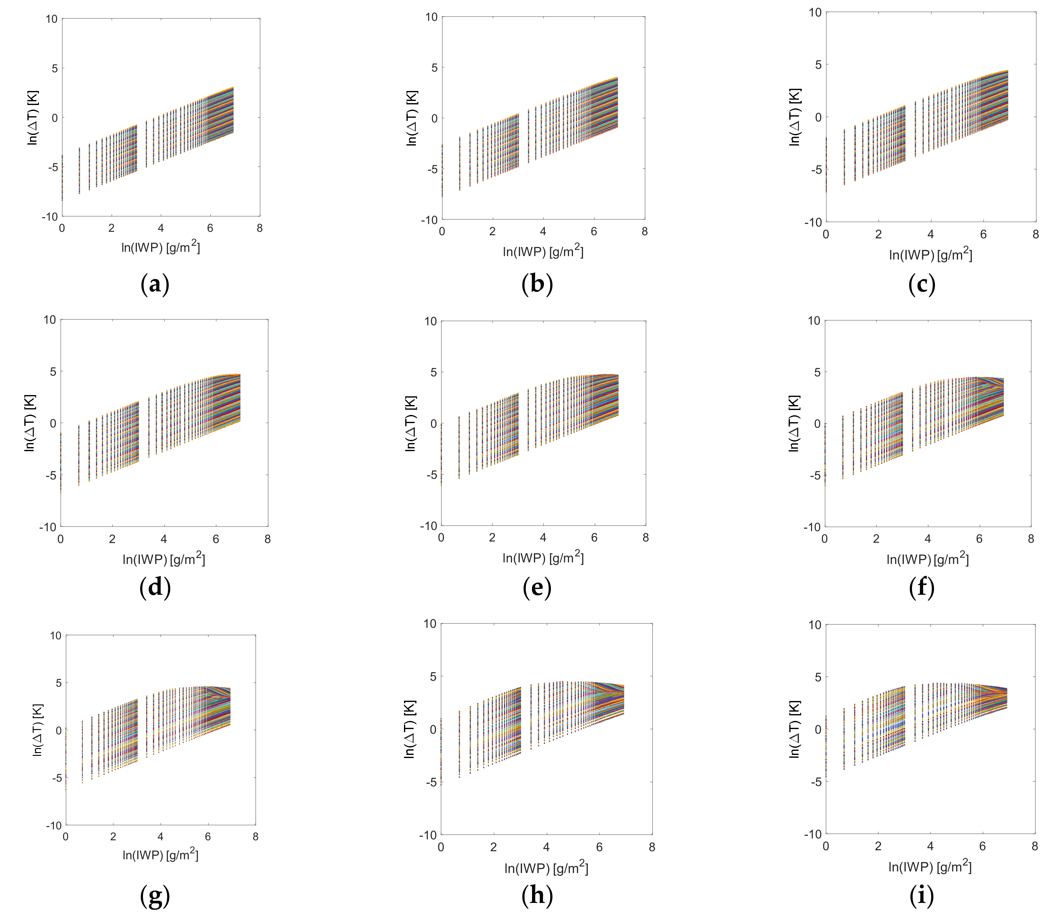
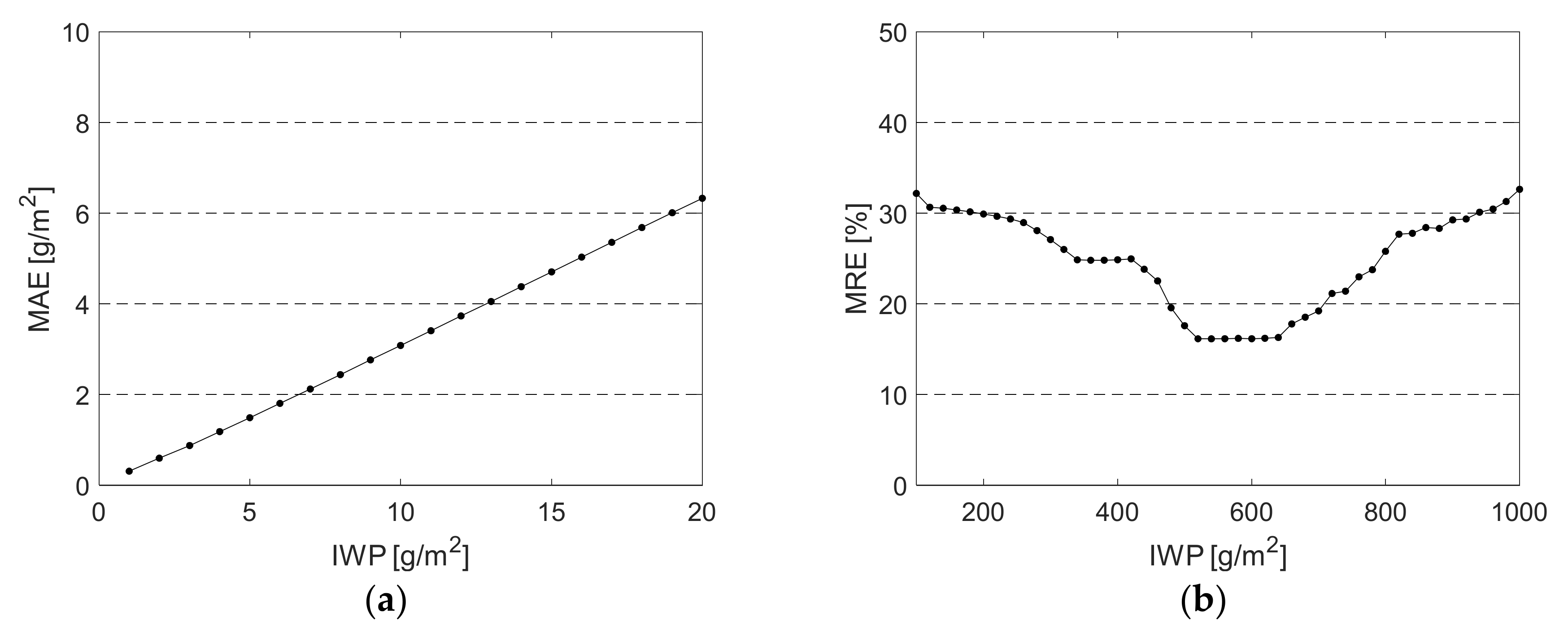
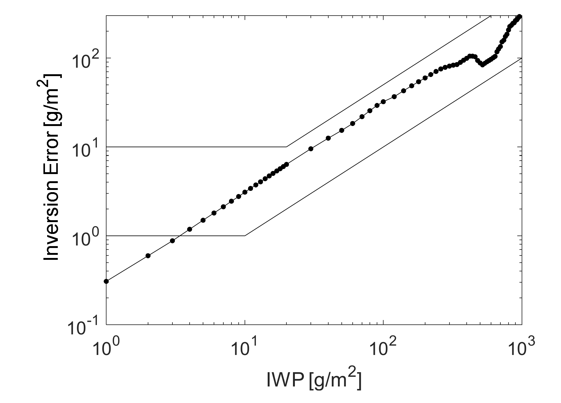
4.2. Inversion Error Analysis

Although the combination of multiple channels can eliminate most of the effects of particle size and cloud height on the brightness temperature difference, the irrelevant factors will still have some influence on the inversion of the ice water path, so further evaluation is needed. The effect of the inversion can be quantitatively evaluated by comparing the value of the regression inversion with the true value of ice water path. In order to avoid the influence of the presence of outliers, the median error is used instead of the standard deviation, which is more robust against rare outliers than root mean square (RMS) error [25]. The value of the ice water path has a large dynamical range, therefore, the evaluation of low IWP value uses the median absolute error (MAE), and the high IWP value uses the median relative error (MRE) [11], that is

$$MAE=median(|{\widehat{x}}_i-x_i|)$$

(6)

$$MRE=median(\frac{|{\widehat{x}}_i-x_i|}{x_i}\times 100\%)$$

(7)

where, ${\widehat{x}}_i$ is the i-th value of the retrieved IWP, and $x_i$ is the i-th true value.

Figure 7 shows the retrieval performance of multi-channel regression method for different ice water paths. It can be seen that the median relative error for high IWP is generally within 10–30%, the inversion error tends to deteriorate at the extremes of the retrieval ranges on both sides, the middle range is smaller, and the minimum is 16.1% at 540 g/m². This is because when the ice water path is low, the detected signal of brightness temperature difference is also weak, and when the ice water path is high, most of the channel’s sensitivity will eventually reach a saturation state. In addition, with the high-frequency channel, the median absolute error is small when the ice water path is less than 20g/m², but the median relative error is relatively larger at 100–300 g/m². Due to the strong scattering effect of high-frequency channel, it is more sensitive to the low ice water path. However, for the lower or thicker clouds, it will cause an opacity to the atmosphere, and only a part of atmospheric columns with ice water content can be sensed.

Buehler et al. have proposed a formal scientific mission requirement based on current background and early research. Figure 8 shows the inversion errors for different values of IWP in logarithmic scale. The solid black lines depict the accuracy requirements, which denote a 1–10 g/m² requirement range for low IWP and a 10–50% relative requirement range for high IWP, respectively [25], and the inversion error of the fitting equation is also drawn in the figure. It can be seen that the errors are always within the acceptable range of accuracy requirements. In particular, the inversion error of low ice water path is relatively small, indicating that the multi-channel regression method for the inversion of ice water path can achieve the expected scientific mission objectives.

5. Conclusions

First, using several selected representative channels in terahertz band, simulations and analysis were carried out under the clear-sky and ice cloudy-sky respectively. More attention was paid to compare the different responses of different channels to the microphysical parameters of ice clouds. Without the prior physical characteristics of ice clouds, the retrieval database cannot be constructed. Therefore, a simple statistical method of multi-channel linear regression analysis was used, realizing a more efficient inversion of ice water path. For the detection of ice clouds by terahertz wave, we usually choose water vapor or oxygen absorption lines and window regions as the inversion channels. Moreover, different offsets were set to detect more information of ice clouds, since different frequencies have different sensitivities to microphysics of ice clouds. High frequencies are sensitive to small particle sizes and low ice water paths, while low frequencies are opposite. When considering the superposition effect of the two microphysical parameters (ice water path and particle size), and one macroscopic physical parameter (cloud height), multiple channels can be selected for fitting to find the optimal combination. The regression equation has a fit degree of 0.951, and the inversion error is acceptable.

It should be noted that the simulation of this paper is only theoretically analyzed, and some factors are assumed to be simplified into an ideal situation for easy processing. For example, the ice cloud is assumed to be homogeneous, which will affect the accuracy of the inversion results to some extent. In addition, the actual ice water path and particle size will satisfy certain constraints. Therefore, all the one-to-one correspondences may not necessarily appear in Figure 5. When inverting parameters of ice clouds, it is better to combine the prior information of the ice clouds to eliminate the priori conditions that do not conform to the reality and improve the accuracy of regression. These issues will be further analyzed and resolved in subsequent studies.

References

1. Guerbette, J.; Mahfouf, J.-F.; Plu, M. Towards the assimilation of all-sky microwave radiances from the SAPHIR humidity sounder in a limited area NWP model over tropical regions. Tellus A Dyn. Meteorol. Oceanogr. 2016, 68, 28620. [Google Scholar] [CrossRef]
2. Geer, A.J.; Baordo, F.; Bormann, N.; Chambon, P.; English, S.J.; Kazumori, M.; Lawrence, H.; Lean, P.; Lonitz, K.; Lupu, C. The growing impact of satellite observations sensitive to humidity, cloud and precipitation. Q. J. R. Meteorol. Soc. 2017, 143, 3189–3206. [Google Scholar] [CrossRef]
3. Brath, M.; Fox, S.; Eriksson, P.; Harlow, R.C.; Burgdorf, M.; Buehler, S.A. Retrieval of an ice water path over the ocean from ISMAR and MARSS millimeter and submillimeter brightness temperatures. Atmos. Meas. Tech. 2018, 11, 611–632. [Google Scholar] [CrossRef] [Green Version]
4. Wang, X.; Liou, K.N.; Ou, S.S.C.; Mace, G.G.; Deng, M. Remote sensing of cirrus cloud vertical size profile using MODIS data. J. Geophys. Res 2009, 114. [Google Scholar] [CrossRef] [Green Version]
5. Holl, G.; Eliasson, S.; Mendrok, J.; Buehler, S.A. SPARE-ICE: Synergistic ice water path from passive operational sensors. J. Geophys. Res. Atmos 2014, 119, 1504–1523. [Google Scholar] [CrossRef]
6. Evans, K.F.; Wang, J.R.C.; Starr, D.; Heymsfield, G.; Li, L.; Tian, L.; Lawson, R.P.; Heymsfield, A.J.; Bansemer, A. Ice hydrometeor profile retrieval algorithm for high-frequency microwave radiometers: application to the CoSSIR instrument during TC4. Atmos. Meas. Tech. 2012, 5, 2277–2306. [Google Scholar] [CrossRef] [Green Version]
7. Fox, S.; Lee, C.; Moyna, B.; Philipp, M.; Rule, I.; Rogers, S.; King, R.; Oldfield, M.; Rea, S.; Henry, M.; et al. ISMAR: An airborne submillimetre radiometer. Atmos. Meas. Tech. 2017, 10, 477–490. [Google Scholar] [CrossRef]
8. Evans, K.F.; Walter, S.J.; Heymsfield, A.J.; Mcfarquhar, G.M. Submillimeter-wave cloud ice radiometer: Simulations of retrieval algorithm performance. J. Geophys. Res. Atmos. 2002, 107, AAC 2-1–AAC 2-21. [Google Scholar] [CrossRef]
9. Evans, K.F.; Wang, J.R.; Racette, P.E.; Heymsfield, G.; Li, L. Ice Cloud Retrievals and Analysis with the Compact Scanning Submillimeter Imaging Radiometer and the Cloud Radar System during CRYSTAL FACE. J. Appl. Meteorol. 2005, 44, 839–859. [Google Scholar] [CrossRef] [Green Version]
10. Jiménez, C.; Eriksson, P.; Murtagh, D. First inversions of observed submillimeter limb sounding radiances by neural networks. J. Geophys. Res. Atmos. 2003, 108, D24. [Google Scholar] [CrossRef]
11. Jiménez, C.; Buehler, S.A.; Rydberg, B.; Eriksson, P.; Evans, K.F. Performance simulations for a submillimetre-wave satellite instrument to measure cloud ice. Q. J. R. Meteorol. Soc. 2007, 133, 129–149. [Google Scholar] [CrossRef]
12. Rydberg, B.; Eriksson, P.; Buehler, S.A. Prediction of cloud ice signatures in submillimetre emission spectra by means of ground-based radar and in situ microphysical data. Q. J. R. Meteorol. Soc. 2007, 133, 151–162. [Google Scholar] [CrossRef]
13. Li, S.; Liu, L.; Gao, T.; Shi, L.; Qiu, S.; Hu, S. Radiation characteristics of the selected channels for cirrus remote sensing in terahertz waveband and the influence factors for the retrieval method. J. Infrared Millim. Waves 2018, 37, 60–65. [Google Scholar]
14. Li, S.; Liu, L.; Gao, T.; Hu, S.; Huang, W. Retrieval method of cirrus microphysical parameters at terahertz wave based on multiple lookup tables. Acta Phys. Sin. 2017, 66, 78–87. [Google Scholar] [CrossRef]
15. Li, S.; Liu, L.; Gao, T.; Huang, W.; Hu, S. Sensitivity analysis of terahertz wave passive remote sensing of cirrus microphysical parameters. Acta Phys. Sin. 2016, 65, 100–110. [Google Scholar] [CrossRef]
16. Buehler, S.A.; Mendrok, J.; Eriksson, P.; Perrin, A.; Larsson, R.; Lemke, O. ARTS, the Atmospheric Radiative Transfer Simulator—Version 2.2, the planetary toolbox edition. Geosci. Model Dev. 2018, 11, 1537–1556. [Google Scholar] [CrossRef]
17. Anderson, G.P.; Clough, S.A.; Kneizys, F.X.; Chetwynd, J.H.; Shettle, E.P. AFGL Atmospheric Constituent Profiles (0–120 km); Optical Physics Division, Air Force Geophysics Laboratory: Lexington, MA, USA, 1986. [Google Scholar]
18. Rothman, L.S.; Gordon, I.E.; Babikov, Y.; Barbe, A.; Chris Benner, D.; Bernath, P.F.; Birk, M.; Bizzocchi, L.; Boudon, V.; Brown, L.R.; et al. The HITRAN2012 molecular spectroscopic database. J. Quant. Spectrosc. Radiat. Transf. 2013, 130, 4–50. [Google Scholar] [CrossRef]
19. Hong, G.; Yang, P.; Baum, B.A.; Heymsfield, A.J.; Weng, F.; Liu, Q.; Heygster, G.; Buehler, S.A. Scattering database in the millimeter and submillimeter wave range of 100–1000 GHz for nonspherical ice particles. J. Geophys. Res. 2009, 114, D06201. [Google Scholar] [CrossRef]
20. Yang, P.; Liou, K.N.; Wyser, K.; Mitchell, D. Parameterization of the scattering and absorption properties of individual ice crystals. J. Geophys. Res.Atmos. 2000, 105, 4699–4718. [Google Scholar] [CrossRef]
21. Geer, A.J.; Baordo, F. Improved scattering radiative transfer for frozen hydrometeors at microwave frequencies. Atmos. Meas. Tech. 2014, 7, 1839–1860. [Google Scholar] [CrossRef] [Green Version]
22. John, V.O.; Buehler, S.A. The impact of ozone lines on AMSU-B radiances. Geophys. Res. Lett. 2004, 31, L21108. [Google Scholar] [CrossRef]
23. Eriksson, P.; Ekström, M.; Rydberg, B.; Murtagh, D.P. First Odin sub-mm retrievals in the tropical upper troposphere: ice cloud properties. Atmos. Chem. Phys. 2007, 7, 471–483. [Google Scholar] [CrossRef] [Green Version]
24. Buehler, S. Cloud Ice Water Submillimeter Imaging Radiometer (CIWSIR): ESA Earth Explorer Mission Proposal; University of Bremen: Bremen, Germany, 2005. [Google Scholar]
25. Buehler, S.A.; Jiménez, C.; Evans, K.F.; Eriksson, P.; Rydberg, B.; Heymsfield, A.J.; Stubenrauch, C.J.; Lohmann, U.; Emde, C.; John, V.O.; et al. A concept for a satellite mission to measure cloud ice water path, ice particle size, and cloud altitude. Q. J. R. Meteorol. Soc. 2007, 133, 109–128. [Google Scholar] [CrossRef] [Green Version]
Figure 1. Nadir brightness temperature detected under the clear-sky and ice cloudy-sky. the solid black lines are the water vapor absorption channels, the solid green lines are the oxygen absorption channels, the dashed lines are the window channels.
Atmosphere 10 00437 g001
Figure 2. Brightness temperature difference caused by different particle shapes. (a) 118.75 ± 5.0 GHz (O2). (b) 157.05 ± 2.6 GHz (Window). (c) 183.31 ± 7.0 GHz (H2O). (d) 243.20 ± 2.5 GHz (Window). (e) 325.15 ± 9.5 GHz (H2O). (f) 424.70 ± 4.0 GHz (O2). (g) 448.0 ± 7.2 GHz (H2O). (h) 664.0 ± 4.2 GHz (Window). (i) 874.4 ± 6.0 GHz (Window).
Atmosphere 10 00437 g002
Figure 3. Brightness temperature difference caused by different effective particle sizes. (a) Window. (b) 118.75 GHz (O2). (c) 183.31 GHz (H2O). (d) 325.15 GHz (H2O). (e) 424.70 GHz (O2). (f) 448.00 GHz (H2O).
Atmosphere 10 00437 g003
Figure 4. Brightness temperature difference caused by different ice water paths. (a) Window. (b) 118.75 GHz (O2). (c) 183.31 GHz (H2O). (d) 325.15 GHz (H2O). (e) 424.70 GHz (O2). (f) 448.00 GHz (H2O).
Atmosphere 10 00437 g004
Figure 5. Brightness temperature difference caused by different particle sizes and ice water paths. (a) 118.75 ± 5.0 GHz (O2). (b) 157.05 ± 2.6 GHz (Window). (c) 183.31 ± 7.0 GHz (H2O). (d) 243.20 ± 2.5 GHz (Window). (e) 325.15 ± 9.5 GHz (H2O). (f) 424.70 ± 4.0 GHz (O2). (g) 448.0 ± 7.2GHz (H2O). (h) 664.0 ± 4.2 GHz (Window). (i) 874.4 ± 6.0 GHz (Window).
Atmosphere 10 00437 g005aAtmosphere 10 00437 g005b
Figure 6. Logarithmic plot of brightness temperature difference (ΔT) with ice water path (IWP) at different particle sizes and cloud heights. (a) 118.75 ± 5.0 GHz (O2). (b) 157.05 ± 2.6 GHz (Window). (c) 183.31 ± 7.0 GHz (H2O). (d) 243.20 ± 2.5 GHz (Window). (e) 325.15 ± 9.5 GHz (H2O). (f) 424.70 ± 4.0 GHz (O2). (g) 448.0 ± 7.2 GHz (H2O). (h) 664.0 ± 4.2 GHz (Window). (i) 874.4 ± 6.0 GHz (Window).
Atmosphere 10 00437 g006
Figure 7. The inversion error of different ice water paths. (a) Median absolute error for low ice water path; (b) Median relative error for high ice water path.
Atmosphere 10 00437 g007
Figure 8. The inversion error of multi-channel regression method for different values of ice water path. The solid black lines depict the scientific mission requirements, which denote a 1–10 g/m2 requirement range for low IWP and a 10–50% relative requirement range for high IWP, respectively.
Atmosphere 10 00437 g008