Monitoring Tropospheric Gases with Small Unmanned Aerial Systems (sUAS) during the Second CLOUDMAP Flight Campaign


1
Department of Chemistry, University of Kentucky, Lexington, KY 40506, USA
2
Department of Mechanical Engineering, University of Kentucky, Lexington, KY 40506, USA
*
Author to whom correspondence should be addressed.
Atmosphere 2019, 10(8), 434; https://doi.org/10.3390/atmos10080434
Submission received: 11 July 2019
/
Revised: 23 July 2019
/
Accepted: 25 July 2019
/
Published: 27 July 2019
(This article belongs to the Special Issue Applications of Small Unmanned Aerial Systems (sUAS) in Atmospheric Chemistry and Physics)
Abstract
:Small unmanned aerial systems (sUAS) are a promising technology for atmospheric monitoring of trace atmospheric gases. While sUAS can be navigated to provide information with higher spatiotemporal resolution than tethered balloons, they can also bridge the gap between the regions of the atmospheric boundary layer (ABL) sampled by ground stations and manned aircraft. Additionally, sUAS can be effectively employed in the petroleum industry, e.g., to constrain leaking regions of hydrocarbons from long gasoducts. Herein, sUAS are demonstrated to be a valuable technology for studying the concentration of important trace tropospheric gases in the ABL. The successful detection and quantification of gases is performed with lightweight sensor packages of low-power consumption that possess limits of detection on the ppm scale or below with reasonably fast response times. The datasets reported include timestamps with position, temperature, relative humidity, pressure, and variable mixing ratio values of ~400 ppm CO2, ~1900 ppb CH4, and ~5.5 ppb NH3. The sensor packages were deployed aboard two different sUAS operating simultaneously during the second CLOUDMAP flight campaign in Oklahoma, held during 26–29 June 2017. A Skywalker X8 fixed wing aircraft was used to fly horizontally at a constant altitude, while vertical profiles were provided by a DJI Phantom 3 (DJI P3) quadcopter flying upward and downward at fixed latitude-longitude coordinates. The results presented have been gathered during 8 experiments consisting of 32 simultaneous flights with both sUAS, which have been authorized by the United States Federal Aviation Authority (FAA) under the current regulations (Part 107). In conclusion, this work serves as proof of concept showing the atmospheric value of information provided by the developed sensor systems aboard sUAS.
1. Introduction
A major problem in atmospheric chemistry research is accurately quantifying dynamic emissions in the proximity of pollution sources under wind turbulence [1,2]. The large bandwidth of turbulent flow experienced at the surface of the Earth is a significant contributing factor that makes it difficult to take precise measurements with existing techniques [3]. In consequence, the current techniques for atmospheric sampling in the lowest few hundred meters of the atmospheric boundary layer (ABL) are associated to large uncertainties. The fugitive greenhouse gases (GHGs), i.e., CH4, CO2, N2O, and hydrofluorocarbons (HFCs) from transportation, industry, and livestock are known to increase global radiative forcing and are a significant source of climate change [4,5,6,7]. Other pollutants such as CO, NH3, SO2, NOx, and volatile organic compounds (VOCs) are a health risk in urban environments and a cause of respiratory diseases [8,9,10]. Reports from independently measured experimental values indicate that GHG emissions are significantly higher than modeled from the same source, suggesting that emission estimates of GHG are incomplete and models are associated with large uncertainties [11,12,13]. Reducing the uncertainty of low-altitude (<100 m) trace gas emissions is critical to fully understanding emission processes and implementing sustainable industrial practices. The traditional use of manned aircraft, weather balloons, towers, or satellites does not provide the cost feasibility, ease-of-use, or spatiotemporal resolution (on the order of meters and seconds) necessary to sufficiently sample pollution at the source in a way that will constrain measurement uncertainties in a practical manner [14].
The fast adoption of unmanned aerial vehicles (UAV) for aerial photography, video, and delivering goods has opened the door for new opportunities in atmospheric research. Indeed, the large power demand and heavy weight of established benchtop analytical instrumentation prevent their use for sampling with UAVs. Thus, the challenge for creating sampling platforms employing drones to detect trace gas emissions consists of developing analytical systems within the lightweight payload constraints [14]. For accomplishing the previous objective, the integration of sensor packages into commercially available small UAVs, creating small unmanned aerial systems (sUAS), has been proposed as a promising quantification method [14]. Gas sensing packages are advantageous due to their lightweight, low power consumption, and robust analytical behavior. However, the sensor output must have limited dependences on variable environmental conditions, possess a high selectivity for target analyte, and a sufficiently fast response time to be adequate for field work [14].
This work demonstrates the proof-of-concept of small unmanned aerial systems (sUAS) that are deployed to quantify trace gases in the lowest, most dynamic region of the atmosphere, contributing a tool to constrain existing mixing ratio uncertainties near potential sources. In this research, two different sUAS capable of detecting the trace gases ammonia (NH3), methane (CH4), and carbon dioxide (CO2) are introduced. The first sUAS is a DJI Phantom 3 (DJI P3) quadcopter used to fly vertical profiles, and the second sUAS is a fixed-wing Skywalker X8 used to fly horizontal profiles. The two sUAS are flown simultaneously to provide datasets with the mixing ratios needed to create a box model of trace gases within the flight area. These trace gas measurements are associated to measurements of temperature, relative humidity, pressure, and position (latitude, longitude, and altitude), which enables the evaluation of sensor performance under variable environmental conditions. The datasets presented summarize the results from 32 flights with each sUAS, which were collected between 26 and 29 June throughout the 2017 Collaboration Leading Operational Unmanned Aerial System Development for Meteorology and Atmospheric Physics (CLOUDMAP) [15] field campaign in Oklahoma.
2. Experimental Methods
2.1. Description of Campaign Site
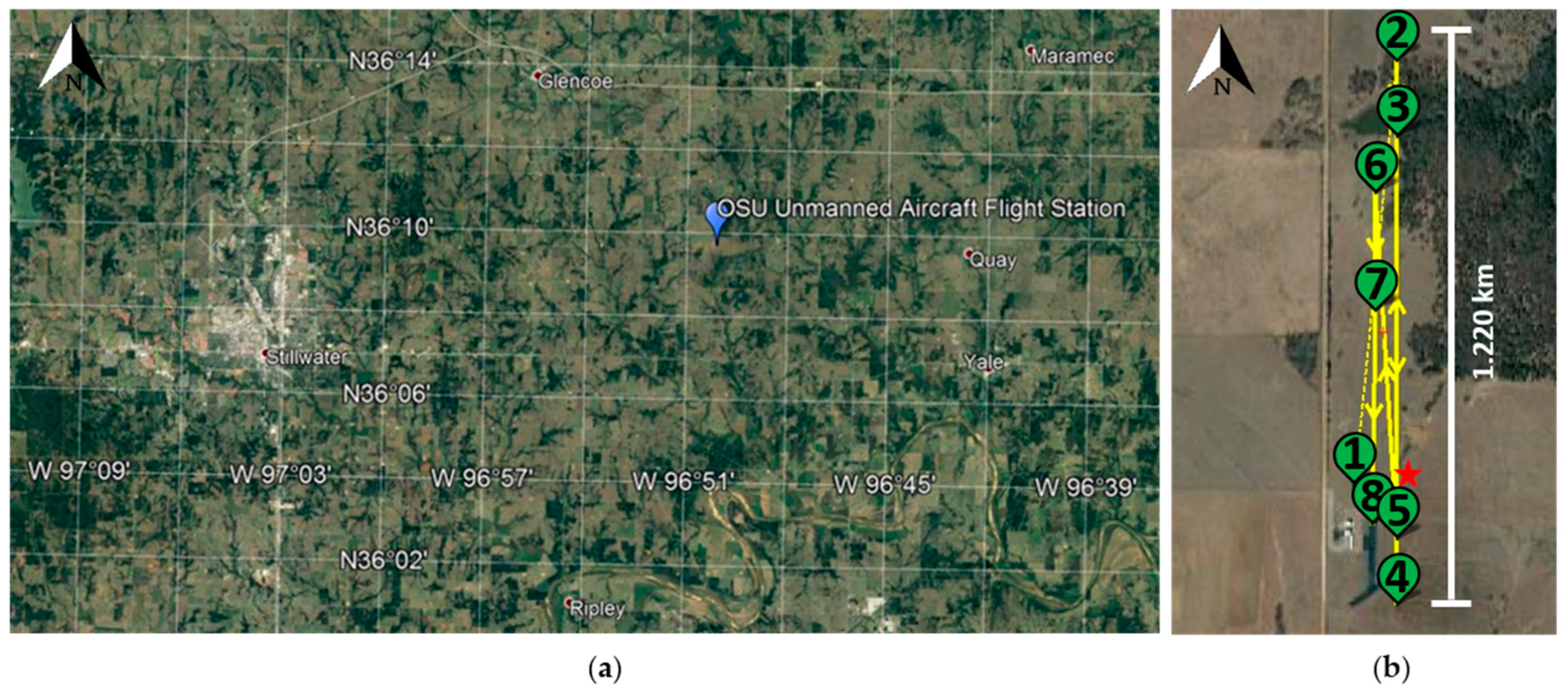
All research flights were performed in accordance with the current regulations (Part 107) established by the United States of America Federal Aviation Authority (FAA) during 26–29 June, 2017. The flights took place at the Unmanned Aircraft Flight Station of Oklahoma State University (317 m above sea-level), which is located ~20 km to the east of Stillwater in the state of Oklahoma (36°09′43″ N, −96°50′07″ W). Figure 1a shows a regional map covering the Oklahoma area, which includes a blue pin indicating the geographical location of the Unmanned Aircraft Flight Station used [16]. The site is 23.72 km from Station 89 (STIL) of the Mesonet network [17], which is used for ground based measurements and sensor validation. The average wind speed at 2 m above ground level (AGL) registered on 27 June was 2.75 (±1.37) m s−1, with the wind direction of 7° N [17]. On 28 June, the average wind speed at 2 m AGL was 4.04 (± 1.09) m s−1, blowing 8° N [17]. Figure 1b shows the distance covered during the flights with the Skywalker X8 aircraft [16] and the actual flight path flown by this aircraft taken from the ground station software (Mission Planner) along with the location of the vertical profiles registered with the DJI P3.
2.2. Description of Flight Patterns
Two different UAVs are flown simultaneously along different flight patterns to demonstrate a method capable of collecting data needed for box models describing the concentration of trace gases. A DJI P3 quadcopter was flown manually to register the vertical profiles, while a Skywalker X8 was flown on autopilot for the horizontal profiles. The vertical profiles data from 10 to 120 m AGL are reported for the ascent and descent rates of 3.0 m s−1. The continuous ascending and descending flight pattern is shown with a black trace in Figure 2a. The battery changes every 15 min were performed to extend the flying time to 1 h. The black line in Figure 2b indicates the fixed coordinates (no horizontal movement) for the global positioning system (GPS) of the DJI P3.
The horizontal profiles at a constant altitude are described by the blue line in Figure 2a. The data reported corresponds to straight trajectory flights (~1.220 km length and ~18 m s−1 airspeed) lasting for ~1 h after reaching 50 m altitude AGL. The data reported corresponds to continuous flying loops between waypoints 2 and 5 in Figure 1b). The GPS trajectories were registered with a VN-300 (VectorNav) during the flights controlled with a waypoint autopilot program on the ground station software (Mission Planner). Figure 2b illustrates the latitudinal changes registered with only minimal longitudinal variations from turning around the UAV. The time series for the flight path of the Skywalker X8 is color coded with a rainbow gradient starting with blue at time zero and shifting toward dark red for the end of the flight (1 h).
2.3. Gas Sensing Packages
Three portable gas sensing packages were developed to monitor the mixing ratio of NH3, CH4, and CO2. A package with microelectromechanical semiconductor (MEMS) sensors allowed monitoring of the gas NH3. Similarly, the second package measured CH4. The third package quantified CO2 levels with a nondispersive infrared detector (NDIR). The payload for the first, second, and third sensing packages were 227, 230, and 181 g, respectively.
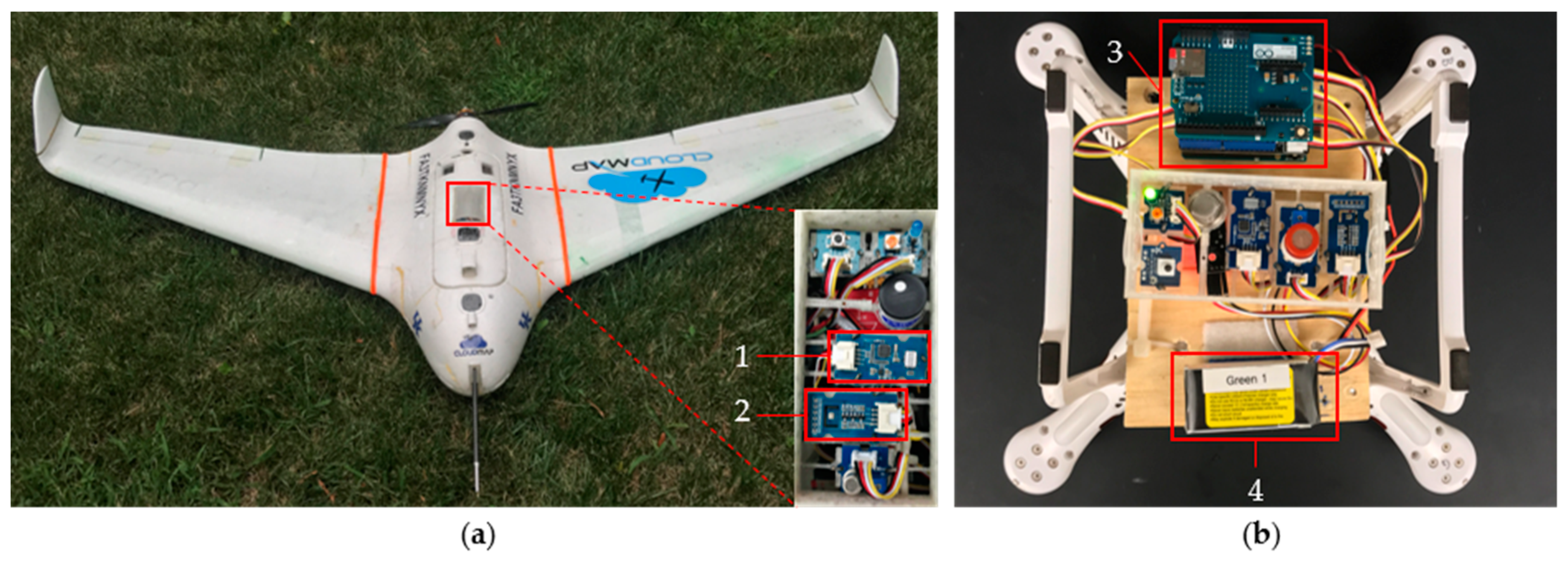
A 10-bit microcontroller (Arduino UNO, Somerville, MA, USA) with a V2 Base Shield (SEEED Studio, Nanshan, China) and a Wireless SD Shield (Arduino) operating at 5.0 V were used to control the sensing packages. Up to 6 h of continuous operation was provided with a 1350 mA h battery (Thunder Power RC 2S, Las Vegas, NV, USA). The data collection set at a rate of 1 Hz was started and stopped with a push-button. The illumination of a light emitting diode (LED) was used to confirm successful data logging for the storage of files in comma separated values (CSV) format to a microSD card with 8 GB capacity (SanDisk Ultra Class 10, Milpitas, CA, USA). The temperature, pressure and percent relative humidity were measured with a BME280 sensor (Bosch, Stuttgart, Germany) with data transmitted via the I2C channel. The mixing ratios for NH3 and CH4 were measured with an I2C MiCS-6814, a 3-channel MEMS semiconducting sensor. For CO2 monitoring, a digital MH-Z16 NDIR sensor was utilized. The calibration curves for the three gases are provided in Figures S1–S3 (Supplementary Information). The operation of the packages was enabled by writing customized codes for the listed sensors. The gas sensing elements were housed and protected in a 3D printed enclosure made of polylactic acid. A pictorial representation of the sensor packages employed and their position in each aircraft is presented in Figure 3. After powering on the sensing packages and re-uploading the code, a time stamp was created. The warm-up and equilibration of the sensors was allowed for at least 1 h before take-off. The results reported below correspond to the flights with identical gas sensing packages placed inside the Skywalker X8 and underneath the DJI P3, as illustrated in Figure 3. For data recovery, the devices were powered down before removing the SD cards.
2.4. Correction for Variable Air Speed and Solar Irradiation
A series of control flights were used to demonstrate that the response of the factory calibrated sensor packages shielded underneath the DJI P3 quadcopter are in excellent agreement with readings at the ground station. The previous controls discarded any possible distortion on the reading of the sensors due to air speed (meaning the rate of motion of the UAV relative to air) or solar irradiation. Small temperature variations were demonstrated not to affect the readout of other sensor packages, which discarded the need for any dynamic in-situ temperature corrections due to temperature fluctuations within a flight. Thus, when the sensor packages were deployed as indicated in Figure 3b, they were shielded from solar radiation with proper aspiration and no further correction to the registered data onboard the DJI P3 quadcopter was required. To test the effect of prop-wash on the sensor package, an experiment was designed to enable simultaneous boundary layer profiles (10–120 m) with a sUAS and tethered weather balloon equipped with the sensor packages. Figures S4–S8 (Supplementary Materials) compare the temperature, relative humidity, methane, carbon dioxide, and ammonia concentration data collected on board the sUAS (black line) and tethered balloon (red line). Figure S9 (Supplementary Information) displays an example for a calibration curve correcting the effect of temperature at different relative humidities. The maximum deviations between the UAV and balloon measurements (Figures S4–S8, Supplementary Information) does not exceed the accuracy figures established in Table A1 and Table A2 (Appendix A). Therefore, it has been concluded from these experiments that the prop wash does not affect the meteorological and trace gas readings on the sensor package on board a quadcopter UAV. However, air speed and solar irradiation introduced a small systematic deviation of the response of sensor packages in the Skywalker X8. The systematic testing demonstrated that the modified behavior onboard the Skywalker X8 was largely created by the air scoop generated over the UV radiation shield enclosing the sensor packages located on top of the aircraft, together with a minor contribution from solar irradiation.
A two-stage set of laboratory controls was designed to correct the response of the sensors for the variable air speed and solar irradiation conditions experienced by the sensor packages onboard the Skywalker X8 during the flights. During the first set of controls, the fuselage of the sUAS carrying the sensors was placed inside a 0.6 × 0.6 × 1.2 m wind tunnel (Model 404B, Engineering Laboratory Design Inc., Lake City, MN, USA) and exposed to a range of wind speeds from 5 to 27 m s−1 to simulate and bracket the effects of airflow over the sensors experienced during data flights with the Skywalker X8. A partial correction factor for the sensor packages that deviated from zero air speeds was obtained.
In the second set of controls, a light source was used to correct for the effects of solar irradiation on the sensor packages protected by a polylactic acid enclosure. For this purpose, a collimated 1 kW high-pressure Hg (Xe) arc lamp was employed to provide actinic radiation in the solar window after removing (1) infrared radiation with a water filter and (2) UV C light with a cutoff filter for wavelength λ ≥ 280 nm [18]. In addition, neutral density filters were employed to attenuate the light and simulate varying levels of sunlight irradiation [19] experienced by the sensor packages in the flight field. A spectral irradiance microspectrometer (Ocean Optics, Dunedin, FL, USA) was used to determine the effective light intensity employed under various attenuations. Thus, a second partial correction factor accounting for the effect of solar irradiation was established for a range of sunlight intensities.
The effect of air speed and solar radiation is modeled and then corrected using MATLAB 2016B. The trace gas mixing ratios are measured systematically over a range of all expected air speeds and solar radiation. The data from these experiments was inputted into a MATLAB script and the effects were observed to determine the overall trends and the relative magnitudes each variable had on every trace gas mixing ratio measured. Next, an algorithm was developed to model all air speeds and solar radiation experienced. Once the effects were well understood mathematically, the deviations were corrected for the appropriate variable. The final overall correction factor combined the partial effects described above by correcting the data sets to an operational air speed of 18 m s−1 and varying the amount of sunlight irradiation.
2.5. Experiments for Data Collection
All data reported was collected between 26 and 29 June, 2017. There were four experiments each day consisting of multiple flights. The temperature, percent relative humidity, and pressure were measured during every flight. A typical experiment lasted for approximately 1 h. For example, the first and second experiments on 28 June, 2017 took place in the intervals 6:04–6:56 a.m. (UTC–5 h) and 7:06–7:57 a.m. (UTC–5 h) to measure NH3 and CH4 respectively. The third experiment only collected physical information and occurred from 8:11 to 9:05 a.m. (UTC–5 h). The first quantification of CO2 was registered during the fourth experiment, which took place in the interval 9:28–10:22 a.m. (UTC–5 h).
2.6. Data Analysis
MATLAB R2016B was used for data processing and plotting. The vertical profile gas measurements up to 120 m altitude AGL were resolved by matching the ascent/descent rate with the data logging rate, creating 40 measurements each per ascent and descent. The reported values in the figures correspond to the average mixing ratio recorded every 3 m altitude [20], with error bars representing one standard deviation. The horizontal profiles were position resolved using the GPS measurements from the VN-300. The GPS data was block averaged to coincide with the 1 Hz logging rate of the trace gas measurements. The figures represent data points averaged every 18 m for latitude or 3 m for altitude depending on the flightpath.
3. Results and Discussion
This section reports data collected during 4 experiments on 28 June, 2017. The physical measurements are presented first, showing the evolution of the temperature and relative humidity during a single flight, and over the course of the four flights. The measurements of the trace gases NH3, CH4, and CO2 are shown later.
3.1. Physical Measurements
The measurements of the temperature, pressure, and percent relative humidity were taken onboard the Skywalker X8 and DJI P3 during each flight. These variables characterize the environment during the flights and facilitate the critical evaluation of sensor outputs that may be affected by varying environmental conditions. The evolution of temperature and relative humidity throughout a single flight, and throughout the early part of the day when major variability exist, is presented next.
3.1.1. Temperature Profiles
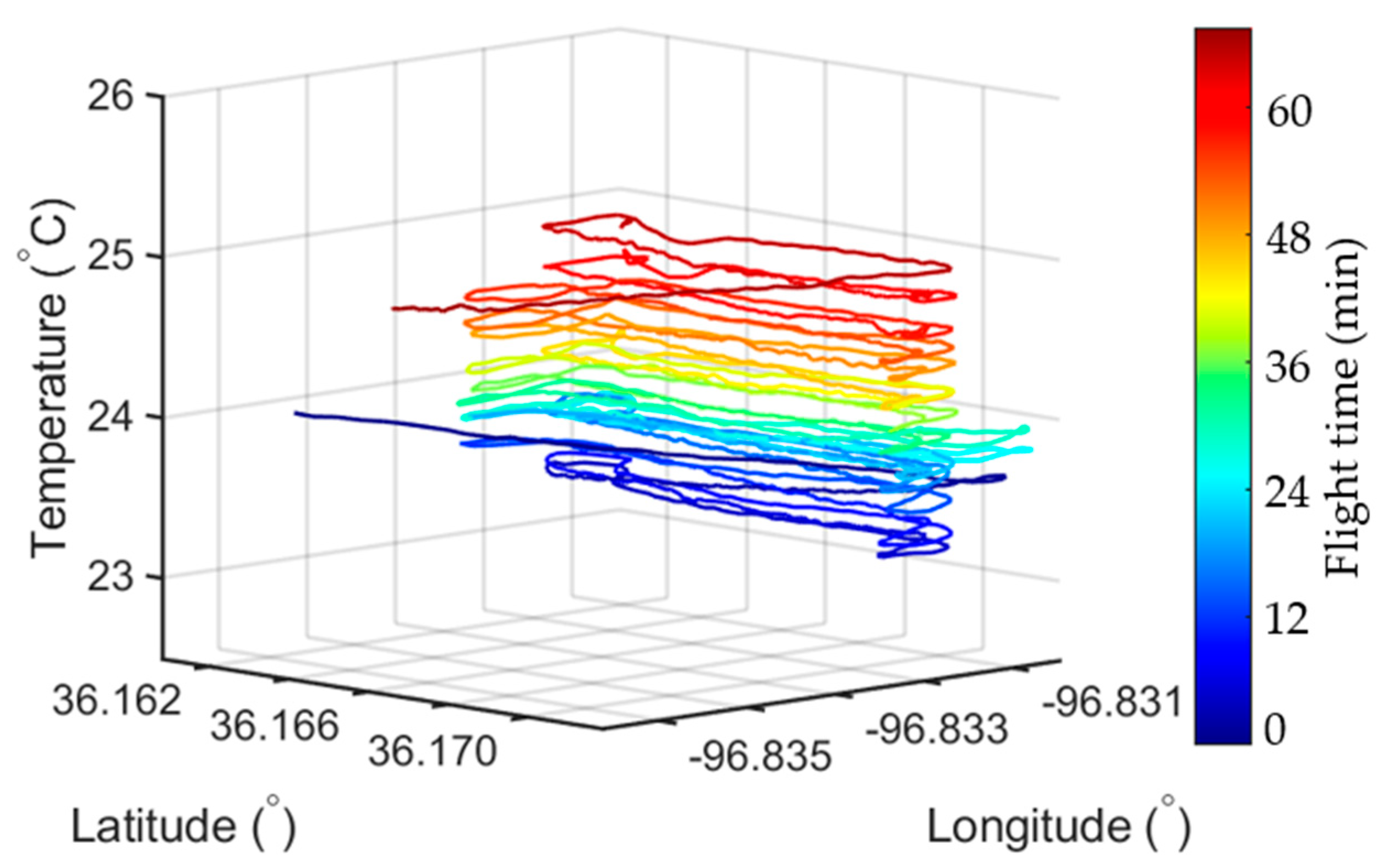
Figure 4 displays an example for a horizontal temperature profile at a constant 50 m altitude AGL during the course of an early morning flight that took off at 7:06 a.m. (UTC–5 h) and landed at 7:57 a.m. (UTC–5 h) on 28 June, 2017. The progression of the flight time is illustrated using a color-bar, which shows blue at the beginning and consistently red-shifts until the conclusion of the flight. For reference, the sun was rising as the Skywalker X8 was completing its 51 min flight path and a continuous increase in the ambient air temperature from 23.3 to 24.8 °C due to increased solar irradiance from the beginning to the end of the flight was captured for this Oklahoma summer sunrise. This small temperature variation neither affected the output of other sensors nor the determination of mixing ratios for trace gases.
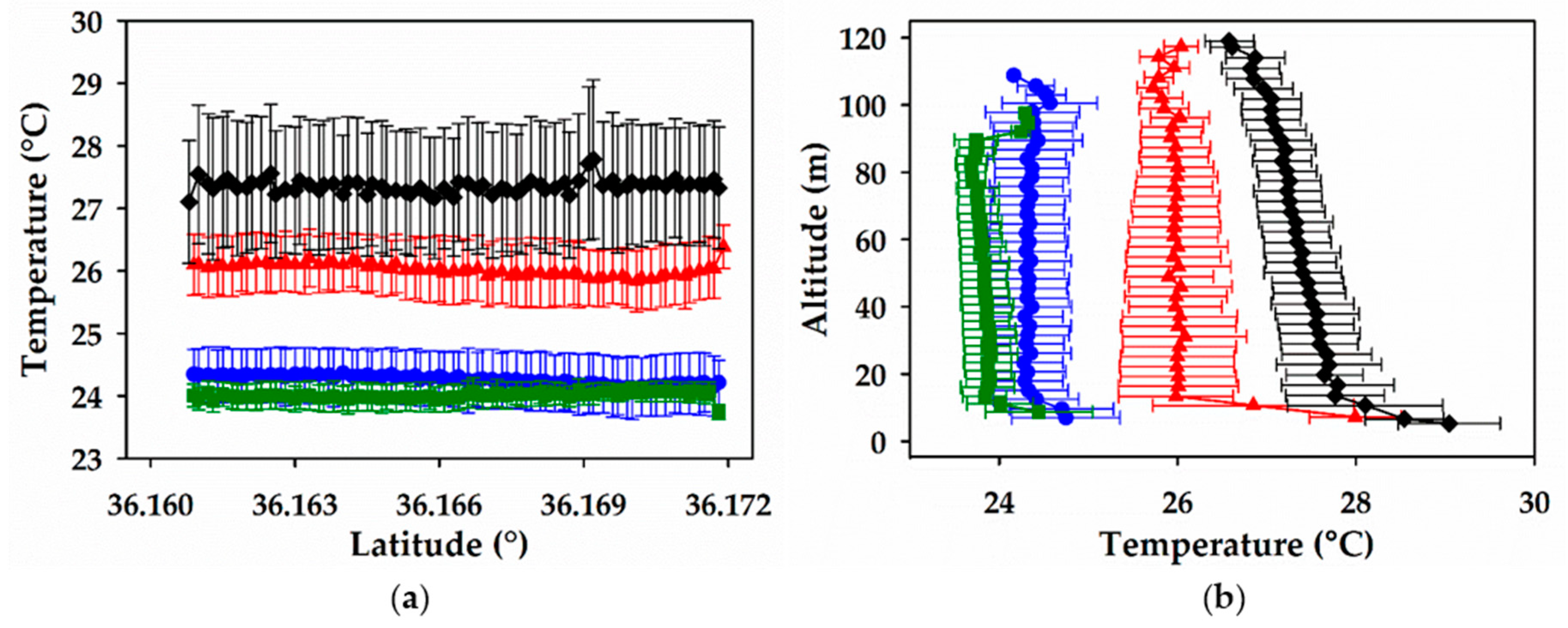
Figure 5 shows the temperature profiles from consecutive flights performed throughout 28 June, 2017, which captured the typical morning temperature inversion resulting from the diurnal cycle. Figure 5a depicts the constant temperature measurements along each horizontal flight path of the Skywalker X8. The four flights took place in the intervals 6:04–6:56 a.m., 7:06–7:57 a.m., 8:11–9:05 a.m., and 9:28–10:22 a.m. (UTC–5 h) and are colored in green, blue, red, and black lines, respectively. From bottom to top in Figure 5a, the mean temperatures are 24.01 (± 0.02), 24.26 (± 0.05), 26.02 (± 0.06), and 27.36 (± 0.12) °C. The variance in the temperature measurements in Figure 5a increases as the day progresses, which reflects an increase in convective turbulent motions due to less stable boundary layer conditions formed as the sun rises and the ground begins to radiate heat. Figure 5b shows the vertical temperature profiles collected onboard the DJI P3 with mean values of (from left to right) 23.88 (± 0.05), 24.36 (± 0.07), 26.04 (± 0.08), and 27.38 (± 0.07) °C.
Figure 5b shows that the first three DJI P3 flights display a relatively stable atmosphere during each flight with practically no temperature change from 15 to 100 m AGL. The greatest temperature gap in the vertical profiles (Figure 5b) occurs between the second and third flights, indicating a warming rate of ~3.5 °C h−1, which coincides with the temperature increment of solar irradiation warming the Earth’s surface. The largest temperature variation and associated uncertainty for each vertical profile (Figure 5b) occurs close to the surface, as expected, due to a reduction in turbulent transport near the surface and reflecting a more inefficient heat exchange by conduction. Overall, reliable temperature readings were provided by both the Skywalker X8 aircraft and the DJI P3 quadcopter.
3.1.2. Relative Humidity Profiles
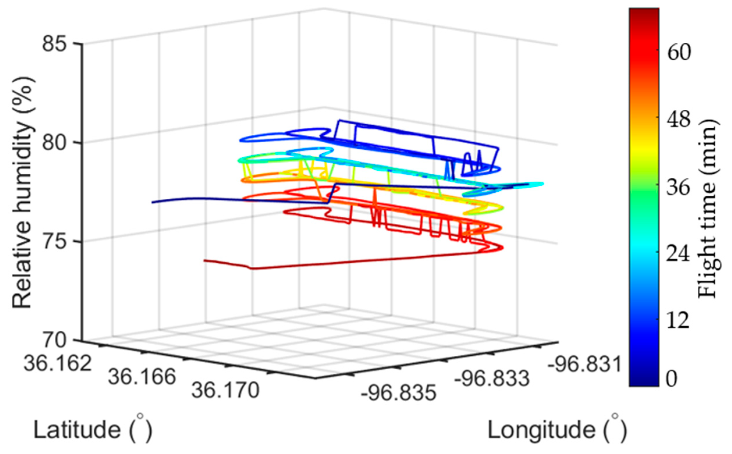
Figure 6 presents an example of a relative humidity horizontal profile recorded simultaneously with the temperature for the same flight in Figure 4 at a constant 50 m altitude AGL. A decrease in relative humidity from 79 to 74% is depicted for the Skywalker X8 flight over time, as shown by the progression from blue to red-shifting of the flight time in the color bar on the right of Figure 6. A direct comparison of Figure 4 and Figure 6 for the 51 min flight indicates the 6.3% relative drop in relative humidity is accompanied by a 6.4% rise in temperature. Thus, a drop in relative humidity is expected with a rise in temperature given that the specific water content does not change.
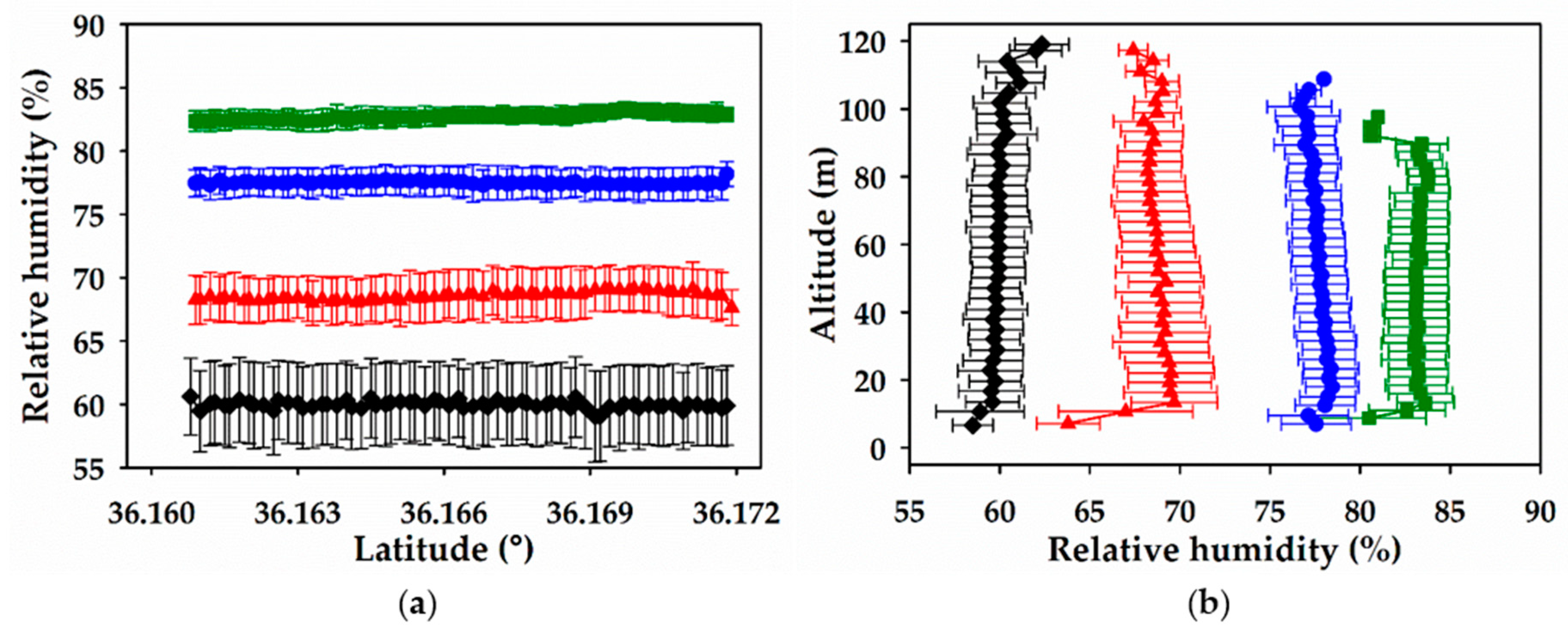
Figure 7 presents the relative humidity measurements for consecutive flights performed on 28 June, 2017, which simultaneously recorded the temperature data shown in Figure 5. Figure 7a shows that the relative humidity remains practically constant within each horizontal flight, while Figure 7b reveals small vertical variations occur with altitude. The data in the horizontal and vertical profiles of Figure 7 clearly illustrates how the relative humidity drops from sunrise to late morning. It is apparent that relative humidity starts to decay near the ground and that as the Earth’s surface begins to warm, the effect is accelerated. As expected, the greatest decrease in relative humidity coincides with the largest increases in temperature. The largest drop of 10.3% in relative humidity is observed between the second and third flights. From top to bottom in Figure 7a, the vertical profiles show relative humidities of 82.96 (± 0.28)%, 77.65 (± 0.25)%, 68.57 (± 0.32)%, and 59.98 (± 0.25)%, respectively. From right to left in Figure 7b, the horizontal profiles display relative humidities of 82.75 (± 0.09)%, 77.51 (± 0.15)%, 68.57 (± 0.23)%, and 59.97 (± 0.39)%, respectively. Similar to the temperature measurements (Figure 5a), an increase in the variance of relative humidity is also evident in Figure 7a, which coincides with the mixing and destabilization of the planetary boundary layer. However, the similar variance of ~0.2% in relative humidity measurements of horizontal and vertical profiles indicates both sUAS employed are reliable platforms for studying this property. Overall, this work demonstrates that the BME280 sensor collects accurate measurements of temperature and relative humidity on board the DJI P3 and Skywalker X8 sUAS.
3.2. Trace Gas Measurements
Trace gases were concurrently measured with physical properties onboard the Skywalker X8 and DJI P3. Three trace gases were quantified during this campaign: NH3, CH4, and CO2. These gases were measured in several flights and gathered in three different groups for practical purposes. NH3 was measured during one set of flights, a different set of flights measured CH4, and a third set of flights measured CO2.
3.2.1. NH3 Profiles
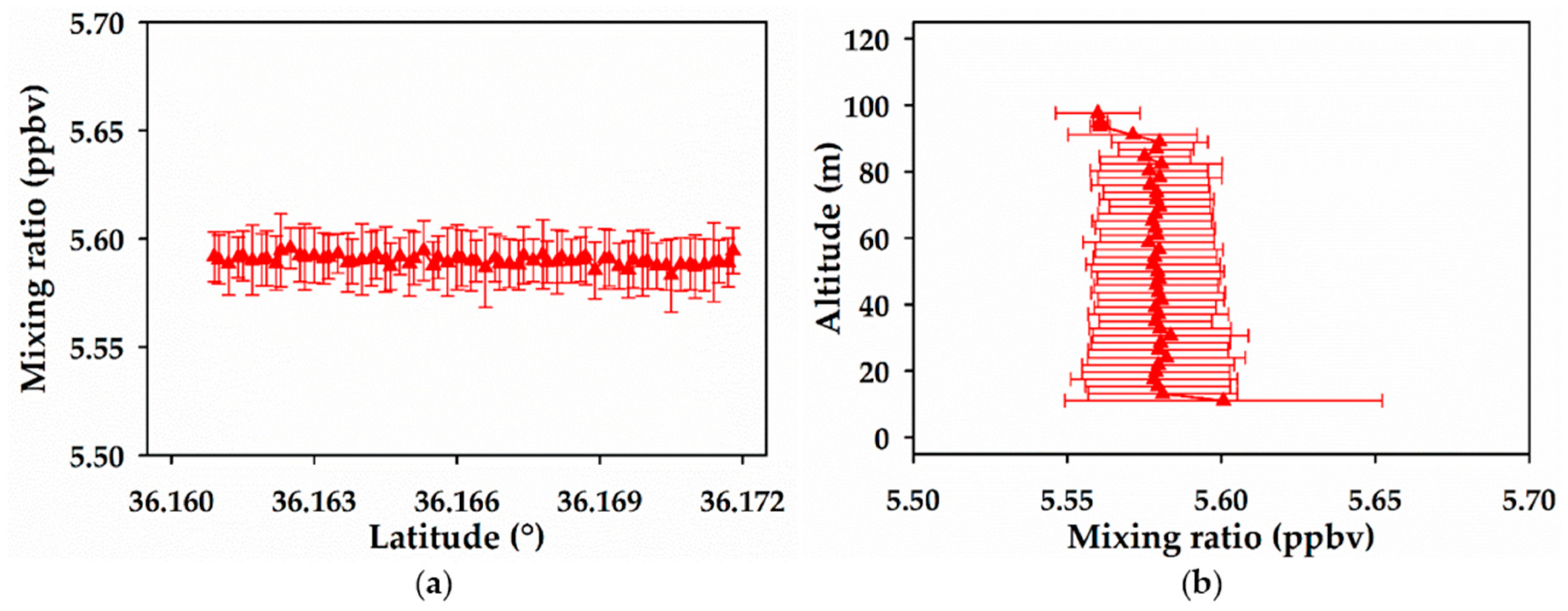
Figure 8 shows an example of the data collected during flights measuring NH3. In this example from the morning of 28 June 2017, the gases were measured from 6:04 to 6:56 a.m. (UTC–5 h) using the Skywalker X8 for the horizontal profiles (Figure 8a), and the DJI P3 for the vertical profiles (Figure 8b). The average mixing ratios measured during the fixed wing flight (Figure 8a) were 5.58 (± 0.01) ppbv NH3. The average mixing ratios detected during rotary wing flights vertical profiling (Figure 8b) were 5.58 (± 0.04) ppbv NH3. The dataset in Figure 8 demonstrates the ability of the MiCS-6814 sensor to accurately detect NH3 at typical tropospheric levels.
3.2.2. CH4 Profiles
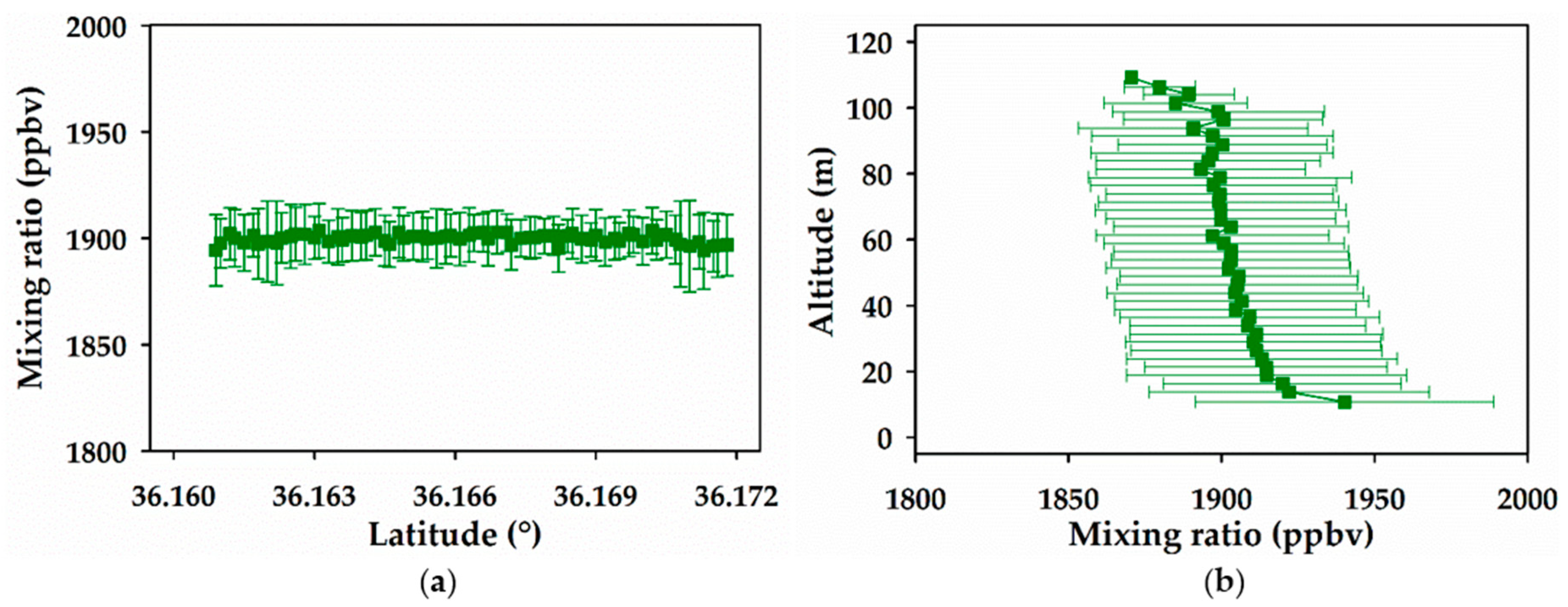
Figure 9 demonstrates the ability of the MiCS-6814 sensor to detect methane, at atmospherically relevant mixing ratios. The example in Figure 9 displays the measured mixing ratios for CH4 from the flights conducted on 28 June, 2017 from 7:06 to 7:57 a.m. (UTC–5 h) using a different channel of the MiCS-6814 sensor. The average mixing ratios for the horizontal profile in Figure 9a were 1892.05 (± 1.49) ppbv CH4, and the corresponding average temperature and relative humidity were 24.26 (± 0.05) °C and 77.51 (± 0.15)%, respectively. For the vertical profiles in Figure 9b, the average mixing ratios were 1892.93 (± 6.76) ppbv CH4, during a flight that averaged a temperature and relative humidity of 24.36 (± 0.07) °C and 77.65 (± 0.25)%, respectively.
3.2.3. CO2 Profiles
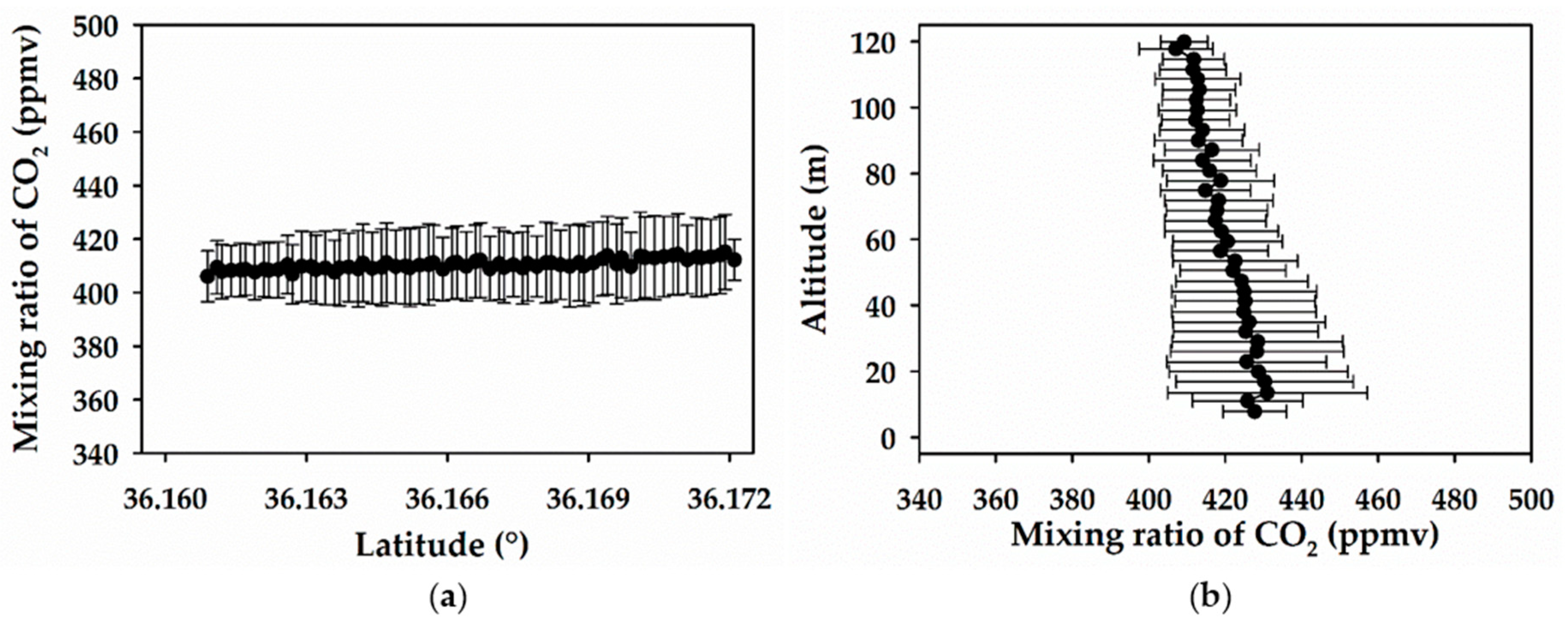
Figure 10 shows how the MH-Z16 NDIR sensor can detect CO2 at atmospherically relevant mixing ratios both during the horizontal and the vertical flights. For example, Figure 10a shows the average mixing ratio of CO2, the temperature, and relative humidity were 411 (± 2), 27.36 (± 0.12) °C, and 59.97 (± 0.39)% for the horizontal profile, respectively. Similarly, the vertical profile in Figure 10b displays an average value of 420 (± 2) ppmv CO2, associated to a mean temperature of 27.38 (± 0.07) °C and an average relative humidity of 59.98 (± 0.25)%.
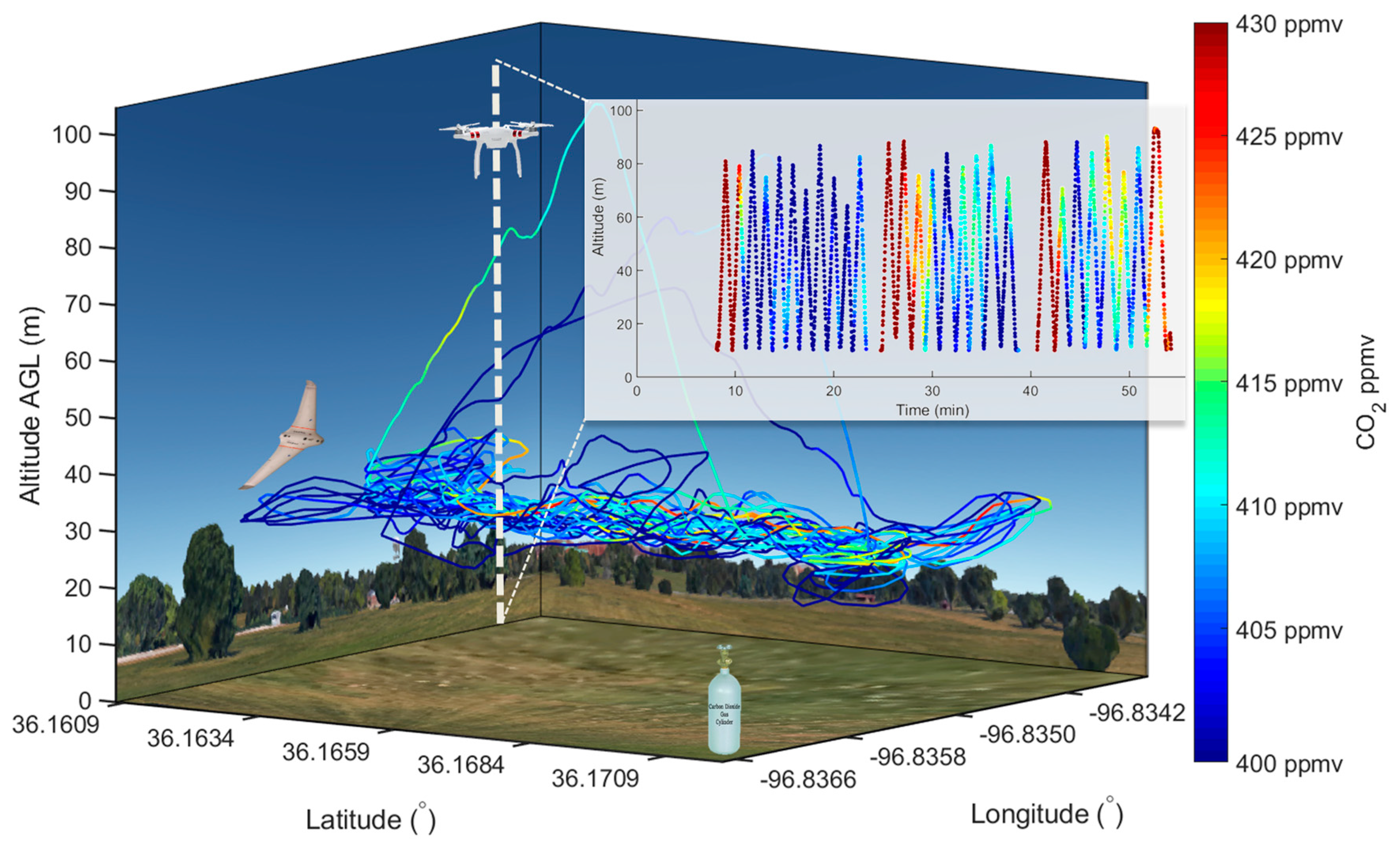
Figure 11 displays the horizontal and the vertical profiles for the detection of CO2 mixing ratios during several programmed gas releases to simulate leaks increasing the environmental background level. Indeed, the work in Figure 11 demostrates that the detection of gas leaks, even as they dilute in the atmosphere, can be monitored employing the developed sensor technology with sUAS.
3.2.4. Environmental Implications of sUAS for Monitoring Trace Gases
Three trace gases (ammonia, methane, and carbon dioxide) were successfully quantified during the second CLOUDMAP flight campaign in Oklahoma. The location of the site and the topography where the flights took place were typical of a rural farmland, what resulted in an optimal combination to measure environmentally relevant mixing ratios of trace gases with the Skywalker X8 and the DJI P3. Remarkably, the similar mixing ratio values registered for each gas at the same altitude (50 m AGL) indicates both platforms are independently robust. For example, based on the data on the integration of repeated measurements presented in Table 1, the differences between the horizontal and the vertical mean mixing ratios at 50 m AGL are 0 ppbv for NH3, 1.3 ppbv for CH4, and 2 ppmv for CO2. In addition, to demonstrate the capability for gas detection at variable altitudes, the mean mixing ratios at 90 and 15 m AGL are provided together with the reference value (RV) determined at the nearby Mesonet. The agreement between the two platforms demonstrates that any effects from air speed and/or solar irradiance has been well understood and corrected to enable consistent measurements with the fixed and rotary wing sUAS. The work also serves as an example showing how this technology can be used to collect the vertical and horizontal profiles of gas levels needed to (1) create a two-dimensional box model covering a slide of 120 km2 per flight and (2) to measure atmospheric composition along extense gasoducts employing sUAS [21] to constrain the region of hydrocarbon leaking during transport.
In addition, the sensor packages provided mixing ratios that were also in excellent agreement with reported values for this region from the Environmental Protection Agency (EPA) and/or the National Oceanographic and Atmospheric Administration (NOAA) of the United States of America [14]. For example, the nearest Ammonia Monitoring Network (AMoN) station (36°55′19″ N, −94°50′20″ W) located approximately 209 km away detected 5.58 ppbv NH3 [22] on 28 June, 2017. The NOAA Atmospheric Radiation Measurement (ARM) site (36°36′25″ N, −97°29′20″ W) about 64 km away from our field campaign site was used to compare CH4 measurements. In addition, on 30 June 2016, the methane levels at the ARM site were 1898.48 ppbv [23]. Lastly, the Mauna Loa weekly average for the week of 25 June, 2017 was 407.71 ppmv [24].
4. Conclusions
A major challenge in quantifying trace gases at low altitudes is the lack of available sampling techniques capable of providing measurements with a spatiotemporal resolution on the order of meters and seconds. Currently, there are not many devices that can be readily incorporated into commercially available UAVs. This work reported the creation and use of trace gas sensor packages integrated into the Skywalker X8 fixed wing and the DJI P3 rotary wing sUAS. The devices were calibrated for environmental conditions and flown at the second CLOUDMAP campaign. The results gathered through a series of example flights described the sensor package’s ability to report temperature and relative humidity evolution throughout a single flight and over the course of several hours. Furthermore, the work analyzed datasets from typical flights and confirmed that the fixed wing and rotary wing platforms provide similar readings, and the trace gas quantifications agree well with relevant EPA and NOAA atmospheric mixing ratios. Therefore, this work has demonstrated that these sensor packages can accurately measure temperature, relative humidity, latitude, longitude, pressure (altitude), ammonia, methane, and carbon dioxide. This device can serve as a useful tool to determine weather conditions and quantify trace gas mixing ratios, particularly at sites of greenhouse and toxic gas pollution. Future applications of this device for environmental monitoring should help to constrain the uncertainty of low altitude (<100 m) trace gas measurements without serious safety concerns or extensive costs. Among the main advantages of the reported analytical platform are the short time needed from set up to deployment (just minutes), and the fact that the analysis can last for up to 1 h covering areas of 120 km2 with high spatiotemporal resolution.
Supplementary Materials
Additional experimental details, Figures S1–S3 for calibration of gases, Figures S4–S8 for tethered balloon validation, and Figure S9 for environmental calibration available online at https://www.mdpi.com/2073-4433/10/8/434/s1.
Author Contributions
M.I.G. proposed the idea for this work; M.I.G., and S.C.C.B. provided the materials; T.J.S. developed the sensor systems and performed all the experimental work under the supervision of M.I.G.; T.J.S. and M.I.G. analyzed the data and wrote the original draft; all authors revised and approved the manuscript.
Funding
This research was supported by the U.S. National Science Foundation under RII Track-2 FEC award No: 1539070, the NASA Kentucky Space Grant Graduate Fellowship Award No: NNX15AR69H, and the NASA R3 EPSCoR award No: 80NSSC19M0032.
Acknowledgments
The authors wish to acknowledge Jamey D. Jacob and the Collaboration Leading Operational Unmanned Aerial Systems Development for Meteorology and Atmospheric Physics (CLOUDMAP) consortium for promoting and sharing knowledge about UASs. Special thanks to Suzanne Weaver Smith for organizing our participation in the campaign that facilitated this work, and to the UK UAV lab personnel for their valuable assistance.
Conflicts of Interest
The University of Kentucky Research Foundation has filed a patent application related to the technology described in this work to the United States Patent and Trademark Office.
Abbreviations
ABL: atmospheric boundary layer; AGL, above ground level; CH4, methane; C3H8, propane; C4H10, butane; CLOUDMAP, collaboration leading operational unmanned aerial system development for meteorology and atmospheric physics; CO, carbon monoxide; CO2, carbon dioxide; DJI P3, DJI Phantom 3; FAA, Federal Aviation Authority; GHGs, greenhouse gases; GPS, global positioning system; LED, light emitting diode; NH3, ammonia; RV, reference values; sUAS, small unmanned aerial systems; UAV, unmanned aerial vehicle; UTC, coordinated universal time; VOCs, volatile organic compounds.
Appendix A

Table A1.
Gas Sensor Specifications.
| Gases | Operating Range (ppbv) | Accuracy (% of Measured Value) | Precision (ppbv) | Resolution (ppbv) |
|---|---|---|---|---|
| Methane | 1000–6000 | ±1.24% | 180 | 10 |
| Ammonia | 500.0–9040 | ±0.20% | 30 | 10 |
| Carbon dioxide | 80,000–1,622,000 | <±1% | <2000 | 1000 |
Table A2.
Meteorological Sensor Specifications.
| Meteorological Variable | Accuracy | Precision | Response Time |
|---|---|---|---|
| Temperature | ±1.0 °C | ±0.005 °C | 0.5 s to 66% full signal |
| Pressure | ±1.0 hPa | ±0.002 hPa | - |
| Relative Humidity | ±3% | ±2% | 1 s to 63% of full signal |
References
- Gimeno, L. Grand challenges in atmospheric science. Front. Earth Sci. 2013, 1, 1–5. [Google Scholar] [CrossRef]
- Watson, A.Y.; Bates, R.R.; Kennedy, D. Mathematical Modeling of the Effect of Emission Sources on Atmospheric Pollutant Concentrations; National Academy of Science: Washington, DC, USA, 1988; Volume 1, p. 704. [Google Scholar]
- Witte, B.M.; Singler, R.F.; Bailey, S.C. Development of an unmanned aerial vehicle for the measurement of turbulence in the atmospheric boundary layer. Atmosphere 2017, 8, 195. [Google Scholar] [CrossRef]
- Rigby, M.; Prinn, R.G.; O’Doherty, S.; Miller, B.R.; Ivy, D.; Mühle, J.; Harth, C.M.; Salameh, P.K.; Arnold, T.; Weiss, R.F.; et al. Recent and future trends in synthetic greenhouse gas radiative forcing. Geophys. Res. Lett. 2014, 41, 2623–2630. [Google Scholar] [CrossRef] [Green Version]
- Köhler, P.; Nehrbass-Ahles, C.; Schmitt, J.; Stocker, T.F.; Fischer, H. A 156 kyr smoothed history of the atmospheric greenhouse gases CO2, CH4, and N2O and their radiative forcing. Earth Syst. Sci. Data 2017, 9, 363–387. [Google Scholar] [CrossRef]
- Pachauri, R.K.; Allen, M.R.; Barros, V.R.; Broome, J.; Cramer, W.; Christ, R.; Church, J.A.; Clarke, L.; Dahe, Q.; Dasgupta, P.; et al. Climate Change 2014: Synthesis Report. Contribution of Working Groups I, II and III to the Fifth Assessment Report of the Intergovernmental Panel on Climate Change; IPCC: Geneva, Switzerland, 2014; p. 151. [Google Scholar]
- Snyder, C.W. Evolution of global temperature over the past two million years. Nature 2016, 538, 226–228. [Google Scholar] [CrossRef] [PubMed]
- Liu, P.; Wang, X.; Fan, J.; Xiao, W.; Wang, Y. Effects of air pollution on hospital emergency room visits for respiratory diseases: Urban-suburban differences in Eastern China. Int. J. Environ. Res. Public Health 2016, 13, 341. [Google Scholar] [CrossRef] [PubMed]
- Dominici, F.; Peng, R.D.; Barr, C.D.; Bell, M.L. Protecting human health from air pollution: Shifting from a single-pollutant to a multi-pollutant approach. Epidemiology 2010, 21, 187–194. [Google Scholar] [CrossRef] [PubMed]
- Nhung, N.T.T.; Schindler, C.; Dien, T.M.; Probst-Hensch, N.; Perez, L.; Künzli, N. Acute effects of ambient air pollution on lower respiratory infections in Hanoi children: An eight-year time series study. Environ. Int. 2018, 110, 139–148. [Google Scholar] [CrossRef] [PubMed]
- Fischer, M. Airborne methane emission measurements for selected oil and gas facilities across California. Environ. Sci. Technol. 2017, 51, 12981–12987. [Google Scholar]
- Lavoie, T.N.; Shepson, P.B.; Gore, C.A.; Stirm, B.H.; Kaeser, R.; Wulle, B.; Lyon, D.; Rudek, J. Correction to assessing the methane emissions from natural gas-fired power plants and oil refineries. Environ. Sci. Technol. 2017, 51, 5856–5857. [Google Scholar] [CrossRef] [PubMed]
- Lee, S.; Choi, Y.; Woo, J.; Kang, W.; Jung, J. Estimating and comparing greenhouse gas emissions with their uncertainties using different methods: A case study for an energy supply utility. J. Air Waste Manag. Assoc. 2014, 64, 1164–1173. [Google Scholar] [CrossRef] [Green Version]
- Schuyler, T.J.; Guzman, M.I. Unmanned aerial systems for monitoring trace tropospheric gases. Atmosphere 2017, 8, 206. [Google Scholar] [CrossRef]
- CLOUDMAP. Collaboration Leading Operational Unmanned Aerial System Development for Meteorology and Atmospheric Physics. Available online: http://www.cloud-map.org/ (accessed on 1 March 2018).
- Google Maps. Stillwater, OK, USA. Available online: https://tinyurl.com/y5euoj5o (accessed on 30 August 2017).
- Mesonet. Stillwater, OK Mesonet Daily Averages. Available online: http://www.mesonet.org/index.php/weather/daily_data_retrieval (accessed on 30 August 2017).
- Zhou, R.; Guzman, M.I. Photocatalytic reduction of fumarate to succinate on ZnS mineral surfaces. J. Phys. Chem. C 2016, 120, 7349–7357. [Google Scholar] [CrossRef]
- Eugene, A.J.; Guzman, M.I. Reactivity of ketyl and acetyl radicals from direct solar actinic photolysis of aqueous pyruvic acid. J. Phys. Chem. A 2017, 121, 2924–2935. [Google Scholar] [CrossRef] [PubMed]
- Hemingway, B.; Frazier, A.; Elbing, B.; Jacob, J. Vertical sampling scales for atmospheric boundary layer measurements from small unmanned aircraft systems (sUAS). Atmosphere 2017, 8, 176. [Google Scholar] [CrossRef]
- Barchyn, T.E.; Hugenholtz, C.H.; Myshak, S.; Bauer, J. A UAV-based system for detecting natural gas leaks. J. Unmanned Veh. Syst. 2018, 6, 18–30. [Google Scholar] [CrossRef]
- Ammonia Monitoring Network; National Atmospheric Deposition Program: Madison, WI, USA, 2016.
- Dlugokencky, E.J.; Lang, P.M.; Crotwell, A.M.; Mund, J.W.; Crotwell, M.J.; Thoning, K.W. Atmospheric Methane Dry Air Mole Fractions from the NOAA ESRL Carbon Cycle Cooperative Global Air Sampling Network; National Oceanic and Atmospheric Administration: Boulder, CO, USA, 2017; pp. 1983–2016.
- Tans, P.; Keeling, R. Trends in Atmospheric Carbon Dioxide at Mauna Loa; Earth System Research Laboratory, National Oceanic and Atmospheric Administration: Boulde, CO, USA, 2016.
Figure 1.
(a) A regional map indicating with a blue pin the flight campaign location. For reference, the grid lines defined by latitude and longitude have a length of ~4.5 km. (b) An aerial photo of the Unmanned Aircraft Flight Station with the distance flown by the Skywalker X8 aircraft. The green pins show the horizontal flight pattern connected by yellow arrowed lines following the progression of numbers covered by the Skywalker X8. The red star indicates the fixed coordinates for vertical profiles registered with the DJI Phantom 3 (DJI P3) quadcopter.

Figure 2.
The flight patterns for data collection versus the altitude above ground level (AGL). (a) The horizontal profile for (blue) Skywalker X8 and (black) vertical profile for DJI P3 aircrafts. (b) The time series for the progression in the global positioning system (GPS) coordinates with altitude for (rainbow color gradient line) the horizontal and (monochromatic black line) vertical flight paths followed by the Skywalker X8 and DJI P3, respectively.

Figure 3.
Unmanned aerial vehicles (UAV) carrying gas sensing packages. (a) Skywalker X8 with (1) MiCS-6814 and (2) BME280. (b) DJI P3 frame with (3) Arduino UNO Microcontroller with V2 Base Shield and Arduino Wireless SD Shield, and (4) battery.
Figure 3.
Unmanned aerial vehicles (UAV) carrying gas sensing packages. (a) Skywalker X8 with (1) MiCS-6814 and (2) BME280. (b) DJI P3 frame with (3) Arduino UNO Microcontroller with V2 Base Shield and Arduino Wireless SD Shield, and (4) battery.

Figure 4.
GPS-resolved temperature measurements along the Skywalker X8 flight path at 50 m AGL from 7:06 to 7:57 a.m. (UTC–5 h) on 28 June, 2017. The color bar to the right hand side represents the progression of time from blue in the beginning to red at the end of this latitudinal flight path.
Figure 4.
GPS-resolved temperature measurements along the Skywalker X8 flight path at 50 m AGL from 7:06 to 7:57 a.m. (UTC–5 h) on 28 June, 2017. The color bar to the right hand side represents the progression of time from blue in the beginning to red at the end of this latitudinal flight path.

Figure 5.
(a) The horizontal and (b) the vertical flight paths measuring temperature variations during the morning of 28 June, 2017 for the times (green square) 6:04–6:56 a.m. (UTC–5 h), (blue circle) 7:06–7:57 a.m. (UTC–5 h), (red triangle) 8:11–9:05 a.m. (UTC–5 h), and (black diamond) 9:28–10:22 a.m. (UTC–5 h).

Figure 6.
GPS-resolved relative humidity measurements along the horizontal flight path during the morning of 28 June, 2017, from 7:06 to 7:57 a.m. (UTC–5 h). The color bar represents the progression of flight time from blue in the beginning to red at the end of the flight.
Figure 6.
GPS-resolved relative humidity measurements along the horizontal flight path during the morning of 28 June, 2017, from 7:06 to 7:57 a.m. (UTC–5 h). The color bar represents the progression of flight time from blue in the beginning to red at the end of the flight.

Figure 7.
(a) The horizontal and (b) the vertical flight paths measuring relative humidity variations during the morning of 28 June, 2017 for the times (green square) 6:04–6:56 a.m. (UTC–5 h), (blue circle) 7:06–7:57 a.m. (UTC–5 h), (red triangle) 8:11–9:05 a.m. (UTC–5 h), and (black diamond) 9:28–10:22 a.m. (UTC–5 h).

Figure 8.
(a) The horizontal and (b) the vertical flight paths measuring the variable mixing ratio of (red triangle) NH3 during the morning of 28 June, 2017 from 6:04 to 6:56 a.m. (UTC–5 h).
Figure 8.
(a) The horizontal and (b) the vertical flight paths measuring the variable mixing ratio of (red triangle) NH3 during the morning of 28 June, 2017 from 6:04 to 6:56 a.m. (UTC–5 h).

Figure 9.
(a) The horizontal and (b) the vertical flight paths measuring the variable mixing ratio of (green square) CH4 during the morning of 28 June, 2017 from 7:06 to 7:57 a.m. (UTC–5 h).
Figure 9.
(a) The horizontal and (b) the vertical flight paths measuring the variable mixing ratio of (green square) CH4 during the morning of 28 June, 2017 from 7:06 to 7:57 a.m. (UTC–5 h).

Figure 10.
(a) The horizontal and (b) the vertical flight paths measuring the variable mixing ratio of CO2 during the morning of 28 June, 2017 from 9:28 to 10:22 a.m. (UTC–5 h).
Figure 10.
(a) The horizontal and (b) the vertical flight paths measuring the variable mixing ratio of CO2 during the morning of 28 June, 2017 from 9:28 to 10:22 a.m. (UTC–5 h).

Figure 11.
The horizontal and the vertical flights for the detection of induced leaks of CO2 (released from the location of the cylinder) during 27 June, 2017 from 1:15 to 2:02 pm (UTC–5 h).
Figure 11.
The horizontal and the vertical flights for the detection of induced leaks of CO2 (released from the location of the cylinder) during 27 June, 2017 from 1:15 to 2:02 pm (UTC–5 h).

Table 1.
Reproducibility analysis and comparison to reference values (RV).
| Total Exp. | Gas | Mean Mixing Ratio (ppbv, except for CO2 that is in ppmv) | ||||
|---|---|---|---|---|---|---|
| Skywalker X8 | DJI P3 | RV | ||||
| 50 m AGL | 50 m AGL | 90 m AGL | 15 m AGL | |||
| 2 | CH4 | 1899.8 (± 5.4) | 1898.5 (± 52.6) | 1855.2 (± 30.1) | 1914.1 (± 59.7) | 1898.4 |
| 2 | NH3 | 5.58 (± 0.01) | 5.58 (± 0.04) | 5.56 (± 0.04) | 5.59 (± 0.05) | 5.58 |
| 3 | CO2 | 409 (± 8) | 407 (± 20) | 405 (± 20) | 409 (± 20) | 407.71 |
© 2019 by the authors. Licensee MDPI, Basel, Switzerland. This article is an open access article distributed under the terms and conditions of the Creative Commons Attribution (CC BY) license (http://creativecommons.org/licenses/by/4.0/).
Share and Cite
MDPI and ACS Style
Schuyler, T.J.; Bailey, S.C.C.; Guzman, M.I. Monitoring Tropospheric Gases with Small Unmanned Aerial Systems (sUAS) during the Second CLOUDMAP Flight Campaign. Atmosphere 2019, 10, 434. https://doi.org/10.3390/atmos10080434
AMA Style
Schuyler TJ, Bailey SCC, Guzman MI. Monitoring Tropospheric Gases with Small Unmanned Aerial Systems (sUAS) during the Second CLOUDMAP Flight Campaign. Atmosphere. 2019; 10(8):434. https://doi.org/10.3390/atmos10080434
Chicago/Turabian StyleSchuyler, Travis J., Sean C. C. Bailey, and Marcelo I. Guzman. 2019. "Monitoring Tropospheric Gases with Small Unmanned Aerial Systems (sUAS) during the Second CLOUDMAP Flight Campaign" Atmosphere 10, no. 8: 434. https://doi.org/10.3390/atmos10080434
Note that from the first issue of 2016, this journal uses article numbers instead of page numbers. See further details here.