Effect of Adding Hydrometeor Mixing Ratios Control Variables on Assimilating Radar Observations for the Analysis and Forecast of a Typhoon

Abstract

The variational data assimilation (DA) method seeks the optimal analyses by minimizing a cost function with respect to control variables (CVs). CVs are extended in this study to include hydrometeor mixing ratios related variables besides the widely used sets of CVs (momentum fields, surface pressure, temperature, and pseudo-relative humidity). The impacts of the extra CVs are investigated in terms of hydrometeor mixing ratios to the assimilation of radar radial velocity (Vr) and reflectivity (RF) for the analysis and prediction of Typhoon Chanthu (2010). It is found that the background error statistics of the extended CVs from the National Meteorological Center (NMC) method is reliable. The track forecast is improved significantly by including hydrometeor mixing ratios as CVs to assimilate radar Vr and RF. The DA experiments using the hydrometer CVs show much improved intensity analysis and forecast. It also improves the precipitation forecast skills to some extent. The positive impact is significant using a direct RF assimilation scheme, when Vr and RF data are applied together. It suggests that when we applying an indirect RF assimilation scheme, the fitting of more hydrometers in the cost function will tend to cause a slight degradation for other variables such as the wind and temperature.

1. Introduction

Variational data assimilation (DA) optimizes the meteorological states by minimizing a cost function with respect to control variables (CVs) that penalizes the observations and first guess fields. Methods for estimating observation errors for various types of observations, especially for the widely used radar observations, are well developed and evaluated based on innovation (observation minus background, OMB) statistics [1]. For the background error covariance (B), the dimension of the B matrix is so large (10⁷ × 10⁷) that it needs to be simplified with the control variable preconditioning procedure. Any prognostic or diagnostic variable can be used as a control variable theoretically. Generally, there are three groups of CVs accounting for the model states [2]: (1) Momentum related CVs such as stream function and velocity potential (ψχ); (2) temperature (T), (3) surface pressure (P), (4) humidity related CVs, such as pseudo-relative humidity (RHs). To better constrain the cost function and optimize the analysis, CVs are adjusted or extended. Sun et al. (2016) applied horizontal UV as CVs to improve convective-scale analyses [3]. Michel et al. (2011) and Descombes et al. (2015) designed a multivariate approach to include hydrometeors in CVs to improve the analyses when assimilating the radar reflectivity and satellite radiance data [4,5].

Doppler weather radar is considered as one of the most outstanding platforms that provide observations with high temporal and spatial resolution [6,7]. Radar observations play an important role in terms of providing tremendous information about velocity fields from radar radial velocity, and about hydrometer fields from radar reflectivity. The determination of the CVs related to the hydrometers is one of the key techniques for radar data assimilation. What is not systematically discussed is how the analyses and forecasts with direct and indirect radar reflectivity data assimilation depend on the hydrometer-related CV options for tropical cyclone (TC) cases. This study serves as a pilot to evaluate the impact of the extra CVs in terms of hydrometeor mixing ratios for radar radial velocity (Vr) and reflectivity data assimilation in the framework of Weather Research and Forecast model data assimilation system (WRFDA). The understanding of the behaviors of the extra CVs, including the hydrometeor mixing ratios related variables, are based on the results for the case of Typhoon Chanthu (2010). Chanthu is one of the most powerful typhoons in 2010, which swept through Wuchuan in Guangdong province. Overall, CNY 5.54 billion (USD 817.7 million) economic losses and nine people killed were reported.

This paper is organized as follows. A brief introduction of the overall WRFDA-3 dimensional (WRFDA-3DVar) system and control variables are described in Section 2. Section 3 describes the experiment design, radar DA configurations, and the typhoon case overview. The results based on different CVs are illustrated in Section 4, before the conclusions and discussions in Section 5.

2. Methodologies

2.1. Cost Function in WRFDA

WRFDA is developed by the National Center for Atmospheric Research (NCAR). The three dimensional variational method [8] of the weather research and forecasting and data assimilation model (WRFDA-3DVar) [9] is designed to obtain a statistically optimal analysis via minimizing a prescribed nonlinear cost function iteratively as:

$$J={(x-x_b)}^T{B}^{-1}(x-x_b)+{(y^o-\mathit{H}(x))}^T{R}^{-1}(y^o-\mathit{H}(x)),$$

(1)

where vectors x and x_b represent the atmosphere states and background states, respectively [10]. y° represents the observation vector. H is the observation operator that maps the model space to the observation space. The background error covariance B and the observation error R are two vital matrixes to constrain the analysis increment.

2.2. The NMC Method

The climatological background error (BE) statistics are estimated using the National Meteorological Center (NMC) method [11]. The NMC method is commonly used to model B, which takes the difference between pairs of forecasts valid at the same time [12]. Plenty of samples based on the forecast differences (for example with 24 and 12 h forecast ranges) are required for the modeling with the NMC method to achieve stable climatological forecast error statistics over a long period (e.g., one month). The background error covariance matrix is expressed as the difference averaged over the time and domain:

$$B\approx \overline{(x^{24}-x^{12})(x^{24}-x^{12}{)}^{\mathrm{T}}}$$

(2)

where $x^{24}$ and $x^{12}$ are 24 and 12 h forecasts, respectively. It is reminded that both of the forecasts contain their errors and that we never have the truth.

$$x^{24}=x^{\mathrm{truth}}+{\mathsf{\epsilon }}^{24}+b^{24}$$

(3)

$$x^{12}=x^{\mathrm{truth}}+{\mathsf{\epsilon }}^{12}+b^{12}$$

(4)

Here, $x^{\mathrm{truth}}$ represents the truth that we never have. $b^{24}$ and $b^{12}$ are the biases in each forecast. ${\mathsf{\epsilon }}^{24}$ and ${\mathsf{\epsilon }}^{12}$ are the random errors. Both 24 and 12 h forecasts are assumed to be unbiased or the bias is constant in time, as $b^{24}$ = $b^{12}$, leading the forecast difference to be:

$$x^{\mathrm{diff}}={\mathsf{\epsilon }}^{24}-{\mathsf{\epsilon }}^{12}$$

(5)

The BE covariance matrix can be modeled as:

$$B\approx \overline{(x^{\mathrm{diff}}){(x^{\mathrm{diff}})}^{\mathrm{T}}}=\overline{({\mathsf{\epsilon }}^{24}-{\mathsf{\epsilon }}^{12}){({\mathsf{\epsilon }}^{24}-{\mathsf{\epsilon }}^{12})}^{\mathrm{T}}}$$

(6)

2.3. B Modeling in WRFDA-3DVar

In the WRFDA-3DVar system, B matrix is usually decomposed as $B=U{U}^T$ so that the preconditioning transform $Uv=x-x_b$ is applied. $\delta x=x-x_b$ represents the analysis increment vector and $v$ stands for control variable vector.

With the following approximation

$$y^o-\mathit{H}(x)\approx y^o-\mathit{H}(x_b)-\mathbf{H}(x-x_b)$$

(7)

where $\mathbf{H}$ is the linearization of the observation operator $\mathit{H}$, Equation (1) can be reshaped in the form of control variable $v$ as

$$J=\frac{1}{2}{v}^{T}v+\frac{1}{2}{(d-\mathbf{H}Uv)}^T{R}^{-1}(d-\mathbf{H}Uv)$$

(8)

where $d=y^o-\mathit{H}(x_b)$ is the innovation vector.

There are five CVs in WRFDA-3DVar that are mostly commonly used. A default option is CV option 5 (CV5) in WRFDA-3DVar. CV5 includes the stream function $\mathsf{\psi }$, the unbalanced part of velocity potential ${\mathsf{\chi }}_{\mathrm{u}}$, the unbalanced part of temperature $T_u$, the pseudo-relative humidity RH, and the unbalanced surface pressure P_su. Another natural choice is to use velocity components (U,V) as control variables for wind analyses (CV option 7; CV7), which includes U component, V component, full temperature (T), full surface pressure (Ps), and pseudo-relative humidity (RHs). The effects of the two momentum control variable options—stream function velocity potential (ψ,χ) and horizontal wind components (U,V)—in radar Vr data assimilation have been discussed in previous studies [13]. To assimilate the hydrometers of radar reflectivity data, the total water qt (sum of water vapor, cloud water, and cloud rain) is used as the moisture CV instead of the RH_s (Xiao et al., 2007) [14]. The total water increments are partitioned into water vapor, cloud water, and cloud rain increments using the tangent and adjoin model of a warm-rain physics.

Microphysical variables including both ice and liquid particles need to be included in the CVs of the cost function to effectively assimilate radar radial velocity and reflectivity data. CVs are extended in this study to include hydrometeor mixing ratios related variables besides the widely used sets of CVs (momentum variables, surface pressure, temperature, and pseudo-relative humidity). The impact of the extra CVs is investigated in terms of hydrometeor mixing ratios (rainwater-q_r, snow-q_s, ice-q_i, graupel-q_g, and cloud liquid-q_c mixing ratio) for radar data assimilation.

The CVs from the two CV options for comparison are summarized as:

CV_7: U, V, P_s, T, q_t

CV_8: U, V, P_s, T, RH_s, q_c, q_r, q_i, q_s, q_g

The transform $\delta x=Uv$ maps the CVs to the analysis variable space through a series of operations $\delta x=U_p{U}_v{U}_{h}v$. Details of the operators $U_p$, $U_v$, and $U_h$ can be referred to Barker et al. (2004) [5]. The $U_h$ is for modeling the horizontal auto-correlation for each control variable, that are assumed to be homogeneous and isotropic using recursive filters. The $U_v$ stands for the vertical transformation by an empirical orthogonal function (EOF) decomposition of the vertical component of BE. In WRFDA-3DVar, the vertical correlations and variances from BE are domain-averaged and constant on each model level. The operator $U_p$ consists in transforming increments of CVs to increments of analysis variables physically.

2.4. Radar Observation Operators

To include the radar observations in the cost function of the WRFDA-3DVar system, the observation operators for radar velocity (Vr) and reflectively (RF) are required. The observation operator for Vr is designed following the formulation in Tong and Xue (2005) [15], as:

$$\mathrm{Vr}=u\cos \alpha \sin \beta +v\cos \alpha \cos \beta +w\sin \alpha$$

(9)

where $\alpha$ radar elevation angle, $\beta$ is the azimuth angle. $u,v,w$ are the three-dimensional wind speeds.

For the reflectivity, the data can be assimilated either directly or indirectly. For the direct RF data assimilation, the operator follows that in Sun and crook (1997) [16], which is expressed as:

$$Z=c_1+c_2{\log }_{10}(\rho {\mathrm{q}}_r)$$

(10)

where Z is the reflectivity factor. The factors of c1 and c₂ are constants with the value of 43.1 and 17.5, respectively. q_r, is the rainwater mixing ratio and $\rho$ is the air density.

One of the problems in the direct radar reflectivity assimilation in WRFDA is that it uses the Z–q_r (reflectivity–rainwater) equation of Equation 10 as the observation operator and a warm-rain partition method to create the hydrometer increments. Nevertheless, WRFDA applies an incremental approach in minimization which requires the linearization of the forward model. The linearization problem will tend to arise, since there is high nonlinearity between Z–q_r, especially when qr is small in a dry background. Thus, a successful direct radar reflectivity assimilation relies largely on other techniques, such as cloud analysis or physical initialization. Another approach is to assimilate the retrieved hydrometers derived from radar RF. The assumption that the in-cloud humidity is saturated is applied to estimate the water vapor following Wang et al. (2013) [17]. Firstly, the in-cloud relative humidity is assumed to be 100% where radar reflectivity is higher than a threshold of 30 dBZ to create the “observation” ${\mathrm{q}}_{\mathrm{v}}^{\mathrm{o}}$ based on the pressure and temperature. For the observation ${\mathrm{q}}_{\mathrm{v}}^{\mathrm{o}}$, the nonlinear observation operator is:

$${\mathrm{q}}_{\mathrm{v}}^{}=rh\times {\mathrm{q}}_{\mathrm{v}\mathrm{s}}^{},$$

(11)

where q_v, rh, and q_vs are specific humidity of water vapor, relative humidity, and saturated specific humidity of water vapor, respectively. The forward model for equivalent radar reflectivity factor relies on the sum of the contributions from pure rainwater q_r, snow q_s, and graupel q_g mixing ratio, following the formulation in Gao et al. (2012) [18],

$$Z_{\mathrm{e}}=Z({\mathrm{q}}_{\mathrm{r}})+Z({\mathrm{q}}_{\mathrm{s}})+Z({\mathrm{q}}_{\mathrm{g}})$$

(12)

3. Experiment Setup

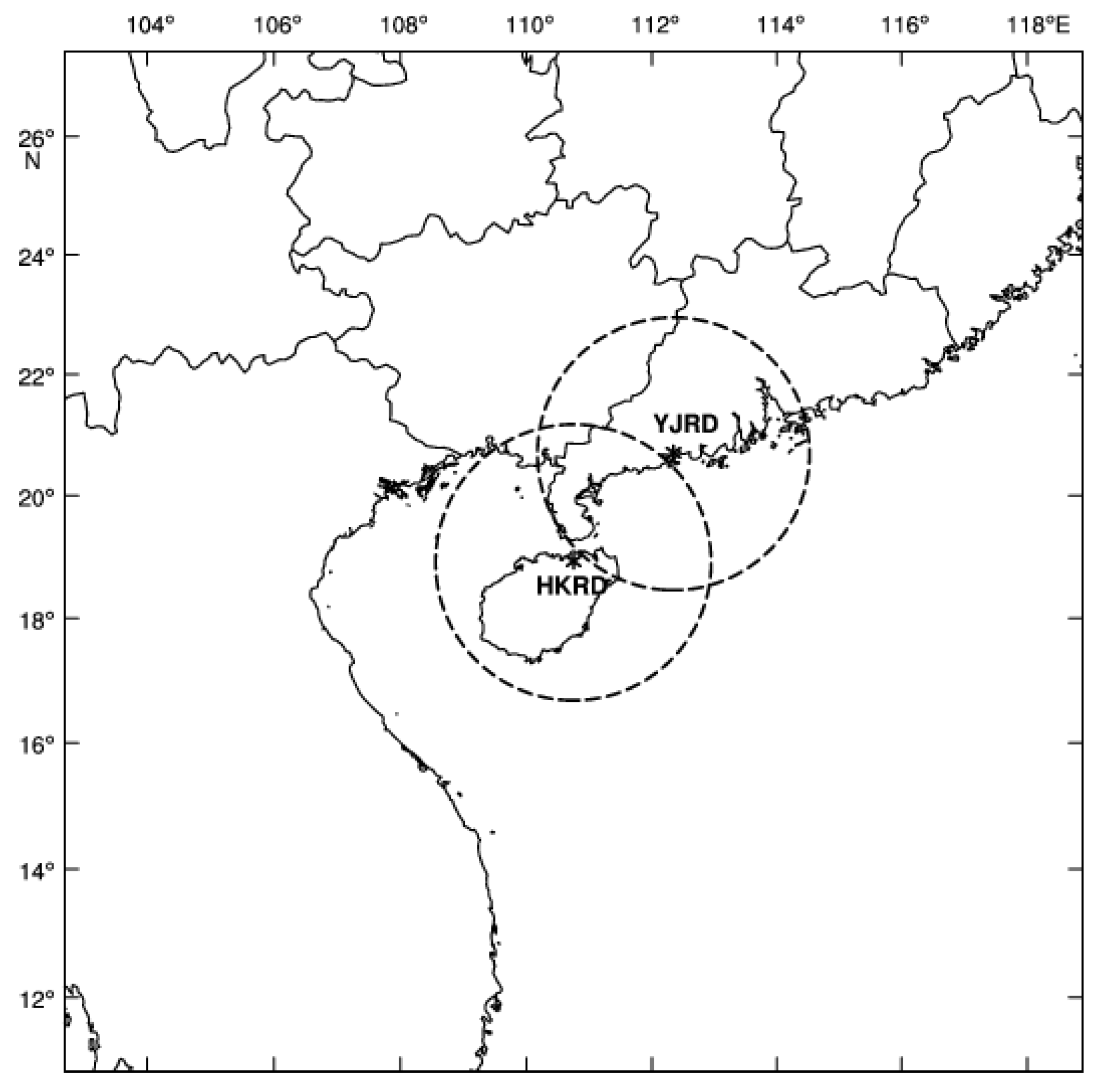
3.1. Radar Observation

The radar observations from coastal WSR-98D radars at Haikou and Yangjiang. The raw data were first preprocessed by an automatic data quality control procedure before assimilation, using the 88d2arps module available in the ARPS [19,20] to correct and remove erroneous observations in terms of Doppler velocity ground clutter removal and de-aliasing. Radar Vr data were further checked and edited manually using the interactive SOLO software [21] from NCAR after the automatic quality control procedures. After quality control was performed, the velocity fields were correctly de-aliased (not shown). The observational error for the Vr and RF data was set as 2 m/s and 5 dBZ following the previous studies of Xiao et al. (2009), Shen et al. (2016), and Shen et al. (2017) [22,23,24].

3.2. Model Configuration and Experimental Design

A single domain was applied in the framework of the WRF model [25] (Skamarock et al. 2008) with 401 × 401 horizontal grids (with 5 km resolution) and 41 vertical levels (with 50 hPa model top), Figure 1. The following physical schemes were employed for the simulation: the Yonsei University scheme (YSU) boundary layer scheme [26] (Hong et al., 2006); the Lin et al. microphysics scheme [27] (Hong et al., 2004); the Kain–Fritsch cumulus parameterization [28] (Kain 1990); the rapid radiative transfer model (RRTM) long-wave scheme and short-wave radiation scheme [29] (Mlawer et al. 1997), and the Noah land surface model for land surface processes scheme.

To investigate the impact of the hydrometer CVs on the analyses/forecasting cyclings, radar DA experiments were conducted every 1 h from 1800 UTC 21 July 2010 to 0000 UTC 22 July (Figure 2), before a deterministic 18 h forecast is initiated from the final DA cycle at 0000 UTC 22 July 2010.

This study conducted three radar DA experiments denoted as RV_RF_CV7, RV_RF_CV8, and RV_RRF_CV8 in

Table 1. Description of the experiments, with radar velocity and radar reflectivity using CV7 (RV_RF_CV7), with radar velocity and radar reflectivity using CV8 (RV_RF_CV8), and with radar velocity and retrieved hydrometers with radar reflectivity using CV8 (RV_RRF_CV8).

Exp Name	Data	CV Type
RV_RF_CV7	RV, RF	CV7
RV_RF_CV8	RV, RF	CV8
RV_RRF_CV8	RV, hydrometers from RF	CV8

. The first two experiments differ based on whether extended CVs were included when radar reflectivity was assimilated directly. For the third experiment, RV_RRF_CV8, the hydrometers retrieved from the reflectivity data were assimilated with CV8 to include the hydrometer CVs.

4. Results

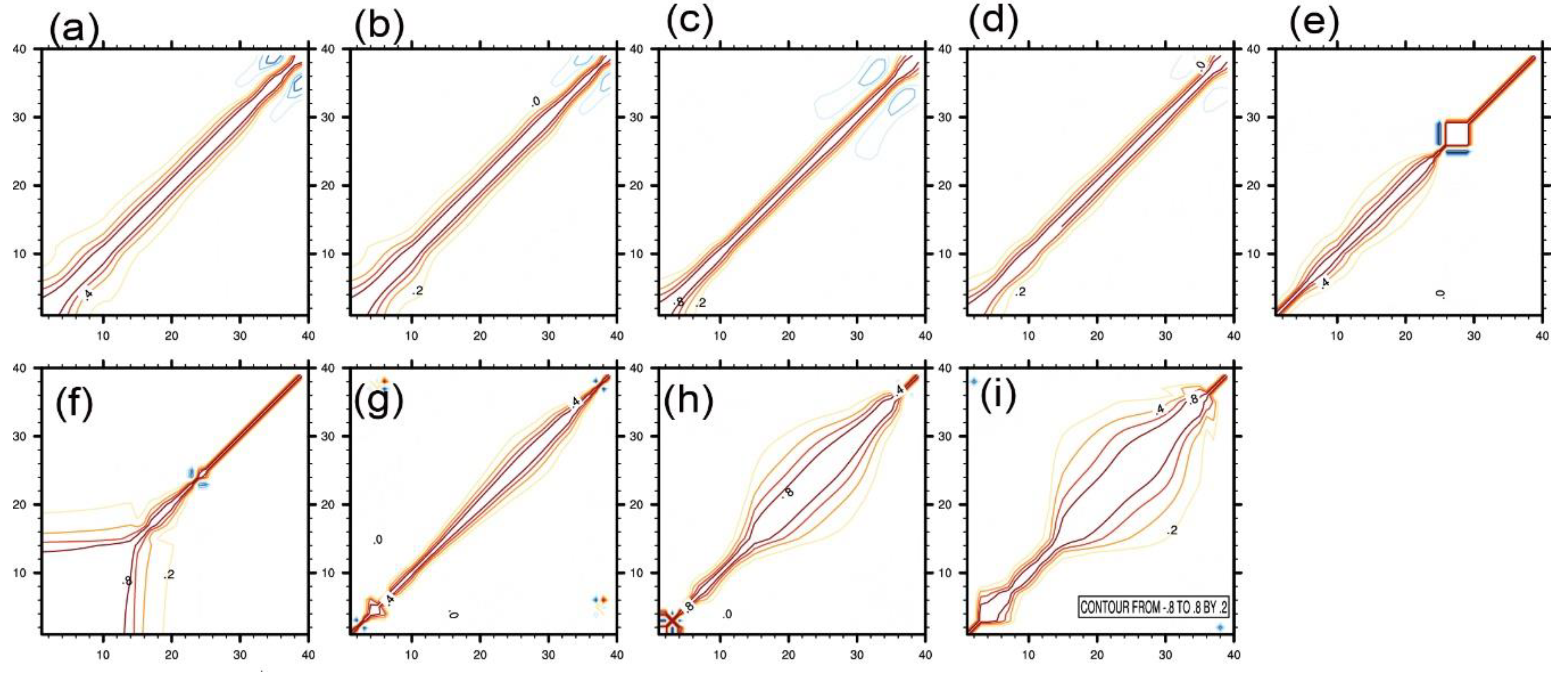
4.1. The Background Error Statistics

The characteristics of the climatological background error from the NMC method are illustrated before the DA experiments were conducted. The standard deviations in the estimated background error matrix for CVs are shown in Figure 3. There were assumptions that the BE statistics of variance and length scale for the control variables are homogeneous and isotropic so that they only vary with heights. The vertical distributions of the standard deviation for the background error (Figure 3) reflect those corresponding features of the profiles for the fields. For example, there are maximum errors at or near the tropopause level for the wind and temperature (around vertical level 30), which was also found in Zhang et al. (2011) [30]. The errors of the snow and graupel mainly appear in more higher levels (>level 17) than that of rainwater (level 10).

Figure 4 shows the vertical correlation of each control variable. The vertical correlations can be large at the associated precipitation levels. The vertical correlations were relatively larger for lower levels for wind and temperature. For solid hydrometers (q_i, q_s, q_g) therewere larger correlations for higher levels (level > 25), while the vertical correlation is larger for lower levels for q_r (level close to 20). These vertical correlations of the hydrometeor errors determine how the information of the observed radar data spread out vertically.

The horizontal correlation length scales of the background errors are shown in Figure 5. It was found that the length scales for the wind fields were around seven to eight grids (~3540 km) and those for the temperature and humidity fields were five grids (~24 km). The length scale for the hydrometers were much smaller with maximum magnitude of one grid (~5 km).

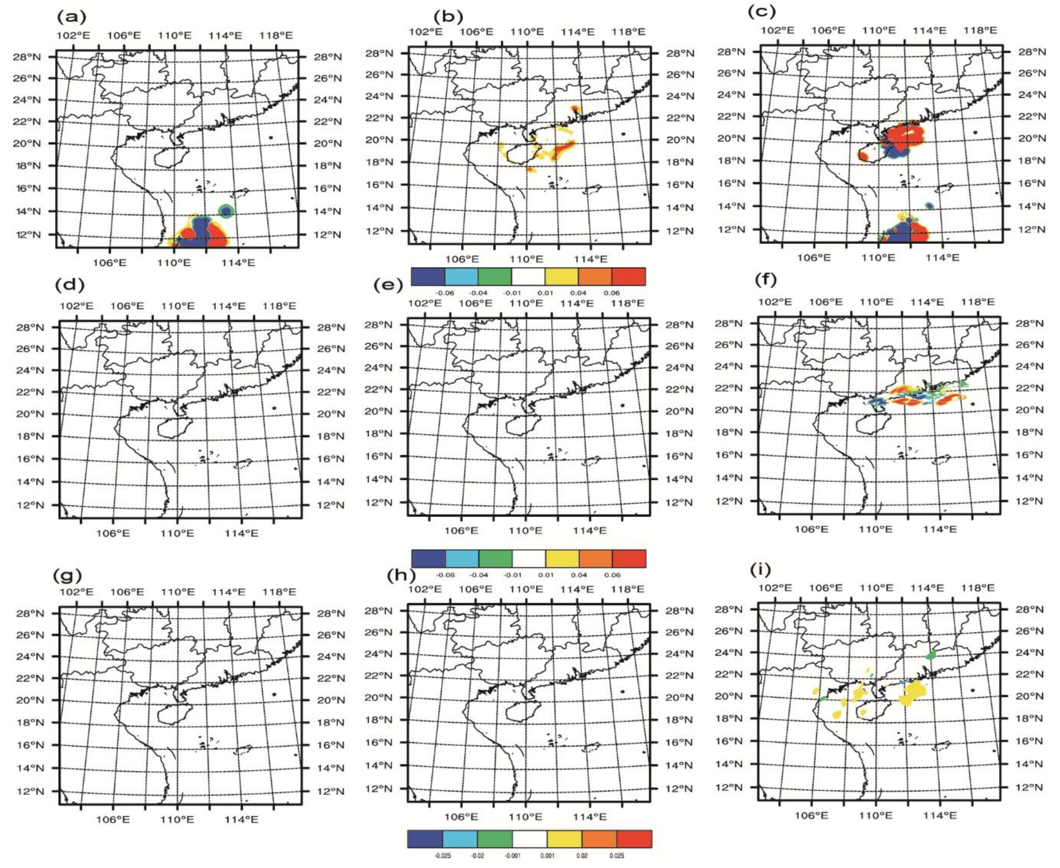
4.2. Analysis Increment

The analysis increments of the column integrated q_r from the first assimilation cycle are illustrated in Figure 6 at 1800 UTC 21 July 2010. The q_r increment from RV_RF_CV7 experiment was close to 0 near the area of the typhoon center in Figure 6a with q_t as CV. Similar dry bias was also found in Wang et al. (2013) when assimilating RF directly [31]. Positive q_r increment was observed near the typhoon center in the neighborhood of Guangdong province in Figure 6b, which can be attributed to the use of the hydrometer-related control variable q_r directly. Noticeable positive increments of q_r were found in RV_RRF_CV8 (Figure 6c) when introducing retrieved hydrometeors in the cost function. The large positive q_r increments from RV_RRF_CV8 was probably introduced by largely fitting the extra retrieved hydrometers, with all hydrometer-related CVs considered. The q_s and q_g increments of RV_RF_CV7 and RV_RF_CV8 were zero, since there was no q_s and q_g information from the observations. Noticeable q_s and q_g increments were observed in RV_RRF_CV8 due to the use of q_s and q_g hydrometers as CV when assimilating the retrieved q_s and q_g information. The increments from the south boundary from RV_RF_CV7 was due to the use of q_t as CV to partition the q_t increments into the q_r increment, which may introduce spurious information to warm hydrometers. For RV_RRF_CV8, the q_r increment from the south boundary was probably related to the overfitting problem when an indirect RF assimilation scheme is applied with CV8. The analysis increments for q_i and q_c were zero for all the experiments, because there is no consideration of q_i and q_c in the observation operator and there is no covariance between q_i and q_c with other CVs.

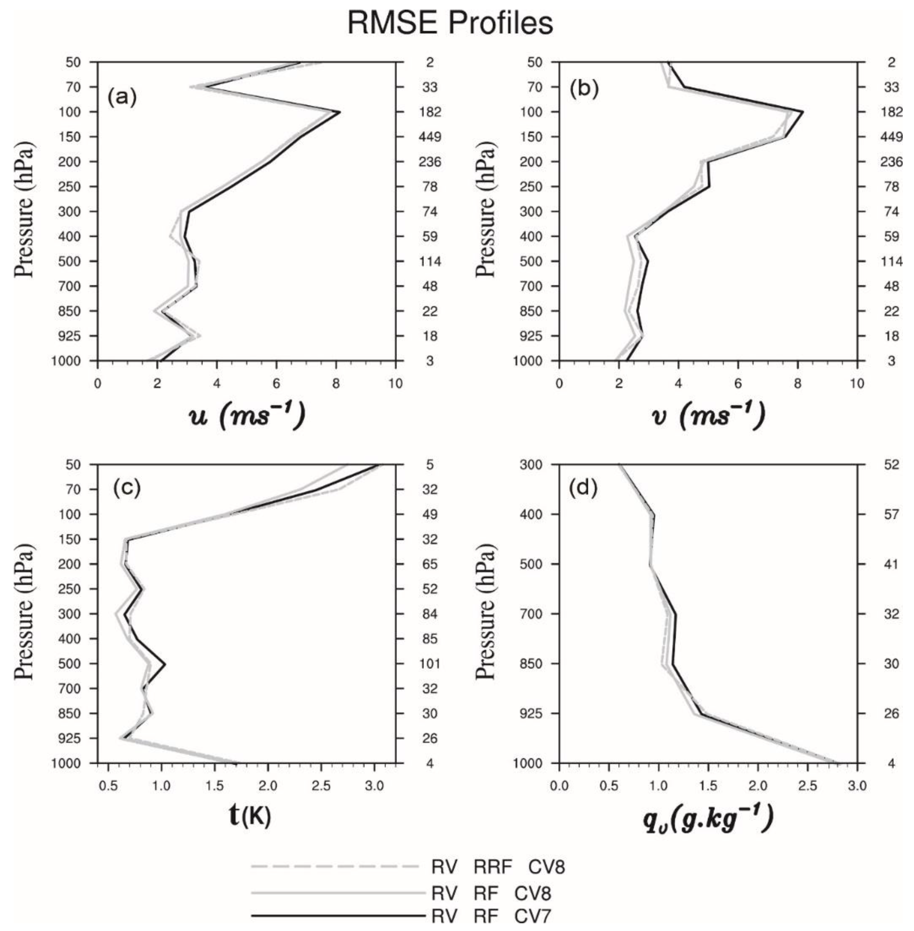
4.3. Verification against the Conventional Observations

Figure 7 shows the vertical profiles of the root mean square error (RMSE) for u-wind, v-wind, temperature, and specific humidity when verifying the analyses against the conventional observations (radiosondes and GeoAMV). The improvement from the radar assimilation with CV8 was observed for most of the fields, while CV7 yielded the largest errors. Generally, RV_RF_CV8 outperforms RV_RRF_CV8 for the wind and temperature. For humidity, smaller RMSE from RV_RF_CV8 was demonstrated at the low troposphere (around 925 hPa) compared with RV_RRF_CV8. The results explain that wind and temperature fields can be improved during the minimization with q_r included in the cost function. It suggests that, when we applying an indirect RF assimilation scheme, the fitting of more hydrometers, such as snow related particles, will tend to cause a slight degradation for other variables such as wind and temperature. It is reported that there is difficulty for the variational DA in obtaining analyses that fit “optimally” to observations representing different scales in one step that minimizes only one cost function (Xie et al., 2011; Tong et al., 2016) [32,33]. Gao et al. (2012) [18] also find that when radar reflectivity is assimilated, the bias errors of the model fields that are related to the reflectivity (such as, rain, snow, and graupel) can be projected onto other model variables (such as wind and temperature) during DA cycles.

Similarly, RMSE for surface variables as 10 m u-wind, 10 m v-wind, 2 m temperature, 2 m q_v, and surface pressure against the conventional observations are illustrated in Figure 8. The improvement from the radar assimilation with CV8 can be seen for the wind and temperature, and 2 m q_v fields. Generally, RV_RF_CV7 yielded the largest RMSE for most of the surface variables.

4.4. Track, Intensity, and Precipitation Forecast

The 18 h track forecasts of Typhoon Chanthu initialized from 0000 UTC 22 July 2010 to 1800 UTC 22 July 2010 are shown in Figure 9a,b to illustrate the impact of the determination of CVs on the TC forecasts. Obvious southward biases were observed from both RV_RF_CV7 and RV_RRF_CV8. The forecast track in the RV_RF_CV8 experiment fited most closely to the CMA (Chinese Meteorological Administration) best track. The method of monitoring TC in CMA can be referred to in Yu et al. (2007) [33] and Song et al. (2010) [34]. RV_RF_CV8 and RV_RRF_CV8 yielded smaller track errors in Figure 8b compared to RV_RF_CV7. For the intensity forecast, the RV_RF_CV8 produced MSLP (minimum sea level pressure) and MW (maximum surface wind speed), thus fitting the best track most closely. The improvement from RV_RF_CV8 was also noticeable to some extent compared with the RV_RF_CV7 in terms of the intensity forecast.

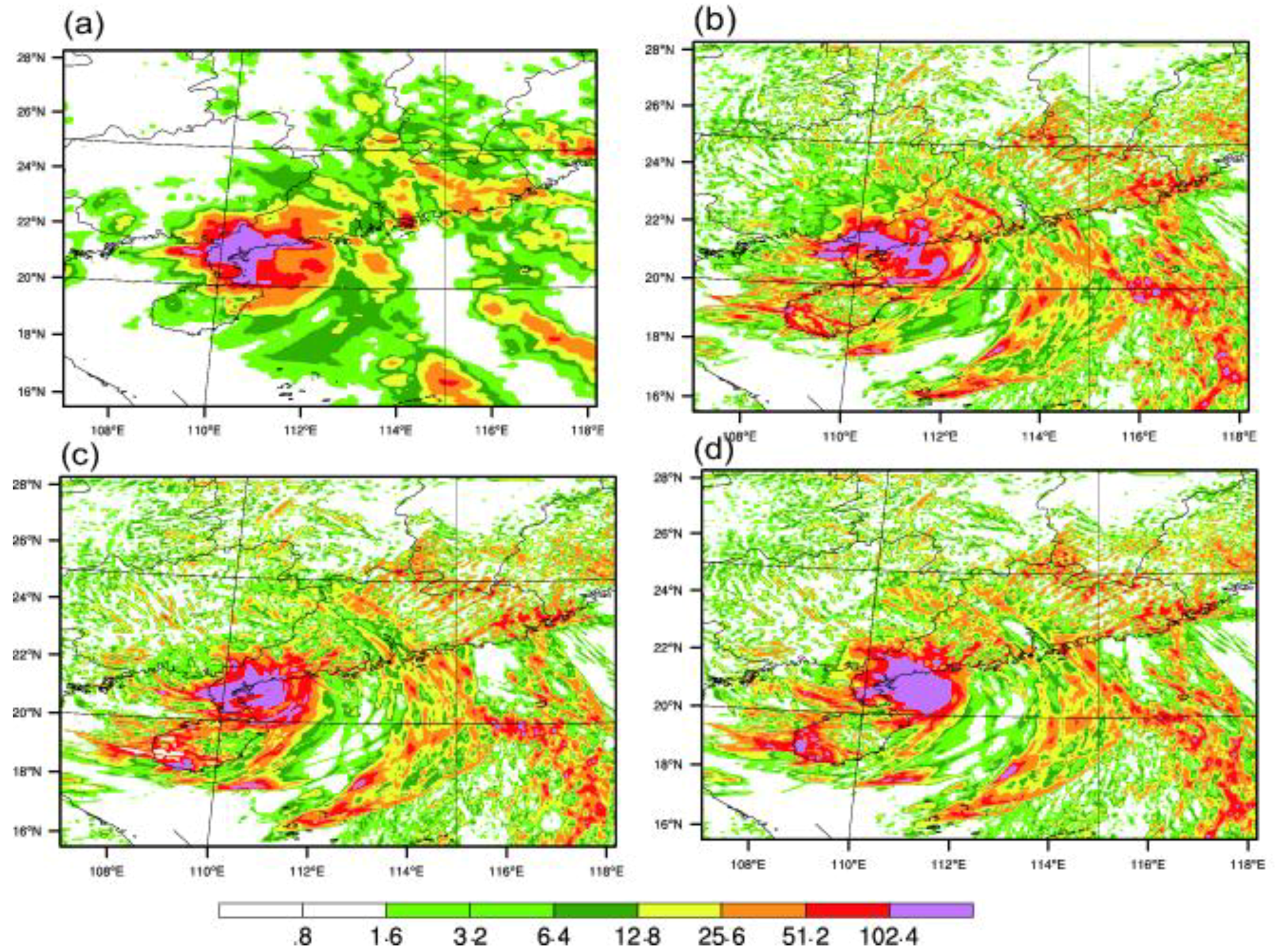
4.5. Precipitation Forecast

Accurate predictions of the precipitation for typhoons are very important for warnings of inland floods. Figure 10 shows the 12 h accumulated precipitation initialized at 0000 UTC 22 July 2010 from the three experiments against the CMA grid rainfall estimation. The rainfall estimation merges the observations from more than 30,000 automatic weather stations of CMA and the rainfall estimates from the NOAA CPC morphing technique (“CMORPH”) [35] (Joyce et al., 2004). It can be seen that the observed maximum exceeded 120 mm in the north of Guangdong Province along the coast from 21° N to 22° N with a nearly square pattern in Figure 10a. The RV_RF_CV7 experiment under predicted the maximum center with a band pattern in Figure 10b. The accumulated precipitation was increased in Figure 10c after assimilating the RF with the retrieved hydrometer using CV8, by extending the CVs in RV_RF_CV8. The significant improvements from RV_RF_CV8 existed in terms of correcting the location and the amount of precipitation. It was found that RV_RRF_CV8 overestimates the maximum of the precipitation in Figure 10d.

The equitable threat scores (ETSs) were calculated for different precipitation thresholds following the metrics in Schaefer 1990 [36] (Figure 11) for the whole domain. Generally, there were higher ETS scores in CV8 than in that in CV7, indicating the advantage of adding extra control variables. For larger thresholds, the ETSs of RV_RF_CV8 and RV_RRF_CV8 were comparable, but the scores from RV_RF_CV8 were consistently superior to RV_RRF_CV8 for smaller thresholds.

5. Conclusions and Perspectives

Control variables are extended in this study to include mixing ratios of hydrometers on top of the widely used sets of CVs (momentum fields, surface pressure, temperature, and pseudo-relative humidity). The impact of the extra CVs is investigated in terms of hydrometeor mixing ratios for radar radial velocity (Vr) and reflectivity (RF) data assimilation. The results are based on the case of Typhoon Chanthu (2010). It is found that the background error statistics of the extended CVs from the NMC are able to reflect those corresponding to the features of the profiles for the fields. The use of hydrometer CVs upgraded the forecast skills of the typhoon track, intensity, and the precipitation to some extent, especially when RF data are assimilated directly along with Vr data. It suggests that, in an indirect RF assimilation scheme, the fitting of more hydrometers (such as snow related particles) tends to cause a slight degradation for other variables (such as wind and temperature).

Although the results are encouraging, there are areas for further improvements and explorations. Further studies with more TCs that are in different regions and at various stages of development are needed for better understanding the impacts of the extra CVs. Our effort in this study represents a step in that direction. To better utilize retrieved hydrometers with various phases (such as from radar reflectivity data), the impacts of individual CVs need to be explored when fitting the observations in the cost function with all sets of control variables and observation types. Therefore, it is important to design a multistep and multiscale DA technique that accounts for the different types and different scales of observations.

References

1. Desroziers, G.; Ivanov, S. Diagnosis and adaptive tuning of observation-error 629 parameters in a variational assimilation. Q. J. R. Meteorol. Soc. 2001, 127, 1433–1452. [Google Scholar] [CrossRef]
2. Xie, Y.; MacDonals, A.E. Selection of momentum variables for a three-dimensional variational analysis. Pure Appl. Geophys. 2012, 169, 335–351. [Google Scholar] [CrossRef]
3. Sun, J.; Wang, H.; Tong, W. Comparison of the impacts of momentum control variables on high-resolution variational data assimilation and precipitation forecasting. Mon. Weather Rev. 2016, 144, 149–169. [Google Scholar] [CrossRef]
4. Michel, Y.; Auligné, T.; Montmerle, T. Heterogeneous convective-scale background error covariances with the inclusion of hydrometeor variables. Mon. Weather Rev. 2011, 139, 2994–3015. [Google Scholar] [CrossRef]
5. Descombes, G.; Auligné, T.; Vandenberghe, F.; Barker, D.M.; Barré, J. Generalized background error covariance matrix model (GEN_BE v2.0). Geosci. Model Dev. 2015, 8, 669–696. [Google Scholar] [CrossRef] [Green Version]
6. Sokol, Z. Effects of an assimilation of radar and satellite data on a very-short range forecast of heavy convective rainfalls. Atmos. Res. 2009, 93, 188–206. [Google Scholar] [CrossRef]
7. Sokol, Z. Assimilation of extrapolated radar reflectivity into a NWP model and its impact on a precipitation forecast at high resolution. Atmos. Res. 2011, 100, 201–212. [Google Scholar] [CrossRef]
8. Courtier, P. The ECMWF implementation of three dimensional variational assimilation (3D-Var). I: Formulation. Q. J. R. Meteorol. Soc. 1998, 124, 1783–1807. [Google Scholar] [CrossRef]
9. Barker, D.M.; Huang, X.Y.; Liu, Z.; Auligné, T.; Zhang, X.; Rugg, S.; Ajjaji, R.; Bourgeois, A.; Bray, J.; Chen, Y.; et al. The Weather Research and Forecasting Model’s Community Variational/Ensemble Data Assimilation System: WRFDA. Bull. Am. Meteorol. Soc. 2012, 93, 831–843. [Google Scholar] [CrossRef]
10. Ide, K.; Courtier, P.; Ghil, M.; Lorenc, A.C. Unified notation for data assimilation: Operational sequential and variational. J. Meteorol. Soc. 1997, 75, 181–189. [Google Scholar] [CrossRef]
11. Parrish, D.F.; Derber, J.C. The national meteorological center’s spectral statistical-interpolation analysis system. Mon. Weather Rev. 1992, 120, 1747–1763. [Google Scholar] [CrossRef]
12. Wang, H.; Huang, X.; Sun, J.; Xu, D.; Zhang, M.; Fan, S.; Zhong, J. Inhomogeneous background rrror modeling for WRF-Var using the NMC method. J. Appl. Meteor. Climatol. 2014, 53, 2287–2309. [Google Scholar] [CrossRef]
13. Li, X.; Zeng, M.; Wang, Y.; Wang, W.; Wu, H.; Mei, H. Evaluation of two momentum control variable schemes and their impact on the variational assimilation of radar wind data: Case study of a squall line. Adv. Atmos. Sci. 2016, 33, 1143–1157. [Google Scholar] [CrossRef]
14. Xiao, Q.; Kuo, Y.; Sun, J.; Lee, W.; Baker, D.M.; Lim, E. An Approach of Radar Reflectivity Data Assimilation and Its Assessment with the Inland QPF of Typhoon Rusa (2002) at Landfall. J. Appl. Meteor. Climatol. 2007, 46, 14–22. [Google Scholar] [CrossRef] [Green Version]
15. Tong, M.; Xue, M. Ensemble Kalman filter assimilation of Doppler radar data with a compressible nonhydrostatic model: OSS experiments. Mon. Weather Rev. 2005, 133, 1789–1807. [Google Scholar] [CrossRef]
16. Sun, J.; Crook, N.A. Dynamical and microphysical retrieval from Doppler radar observations using a cloud model and its adjoint. Part I: Model development and simulated data experiments. J. Atmos. Sci. 1997, 54, 1642–1661. [Google Scholar] [CrossRef]
17. Wang, H.; Sun, J.; Zhang, X.; Huang, X.; Auligné, T. Radar data assimilation with WRF 4D-Var. Part I: System development and preliminary testing. Mon. Weather Rev. 2013, 141, 2224–2244. [Google Scholar] [CrossRef]
18. Gao, J.; Stensrud, D.J. Assimilation of reflectivity data in a convective-scale, cycled 3DVAR framework with hydrometeor classification. J. Atmos. Sci. 2012, 69, 1054–1065. [Google Scholar] [CrossRef]
19. Xue, M.; Wang, D.H.; Gao, J.D.; Brewster, K.; Droegemeier, K.K. The Advanced Regional Prediction System (ARPS), storm-scale numerical weather prediction and data assimilation. Meteorol. Atmos. Phys. 2003, 82, 139–170. [Google Scholar] [CrossRef]
20. Brewster, K.; Hu, M.; Xue, M.; Gao, J. Efficient assimilation of radar data at high resolution for short-range numerical weather prediction. In Proceedings of the WWRP International Symposium on Nowcasting and Very Short Range Forecasting, Toulouse, France, 3 June 2005. [Google Scholar]
21. Oye, R.; Mueller, C.; Smith, C. Software for radar data translation, visualization, editing and interpolation. In Proceedings of the 27th Conference on Radar Meteorology, Vail, CO, USA, 9–13 October 1995. [Google Scholar]
22. Xiao, Q.; Zhang, X.Y.; Davis, C.; Tuttle, J.; Holland, G.; Fitzpatrick, P.J. Experiments of hurricane initialization with airborne Doppler radar data for the advanced research hurricane WRF (AHW) model. Mon. Weather Rev. 2009, 137, 2758–2777. [Google Scholar] [CrossRef]
23. Shen, F.; Min, J. Assimilation of radar radial velocity data with the WRF hybrid ETKF-3DVAR system for the prediction of hurricane Ike (2008). Atmos. Res. 2016, 169, 127–138. [Google Scholar] [CrossRef]
24. Shen, F.; Xu, D.; Xue, M.; Min, J. A comparison between EDA-EnVar and ETKF-EnVar data assimilation techniques using radar observations at convective scales through a case study of Hurricane Ike (2008). Meteorol. Atmos. Phys. 2017, 130, 1–18. [Google Scholar] [CrossRef]
25. Skamarock, W.C.; Klemp, J.B.; Dudhia, J.; Gill, D.O.; Barker, D.M.; Duda, M.G.; Huang, X.Y.; Wang, W.; Powers, J.G. A Description of the Advanced Research WRF Version 3; NCAR Technical Note, NCAR/TN-4751STR; NCAR: Pod, CA, USA, 2008. [Google Scholar]
26. Hong, S.Y.; Noh, Y.; Dudhia, J. A new vertical diffusion package with explicit treatment of entrainment processes. Mon. Weather Rev. 2006, 134, 2318–2341. [Google Scholar] [CrossRef]
27. Hong, S.Y.; Dudhia, J.; Chen, S.H. A revised approach to ice microphysical processes for the bulk parameterization of clouds and precipitation. Mon. Weather Rev. 2004, 132, 103–120. [Google Scholar] [CrossRef]
28. Kain, J.S.; Fritsch, J.M. A one-dimensional entraining/detraining plume model and its application in convective parameterization. J. Atmos. Sci. 1990, 47, 2784–2802. [Google Scholar] [CrossRef]
29. Mlawer, E.J.; Taubman, S.J.; Brown, P.D.; Iacono, M.J.; Clough, S.A. Radiative transfer for inhomogeneous atmospheres: RRTM, a validated correlated-k model for the longwave. J. Geophys. Res. 1997, 102, 16663–16682. [Google Scholar] [CrossRef] [Green Version]
30. Zhang, M.; Zhang, F. E4DVar: Coupling an ensemble Kalman filter with four-dimensional variational data assimilation in a limited-area weather prediction model. Mon. Weather Rev. 2012, 140, 587–600. [Google Scholar] [CrossRef]
31. Xie, Y.; Koch, S.; McGinley, J.; Albers, S.; Bieringer, P.E.; Wolfson, M.; Chan, M. A space–time multiscale analysis system: A sequential variational analysis approach. Mon. Weather Rev. 2011, 139, 1224–1240. [Google Scholar] [CrossRef]
32. Tong, W.; Li, G.; Sun, J.; Tang, X.; Zhang, Y. Design Strategies of an Hourly Update 3DVAR Data Assimilation System for Improved Convective Forecasting. Weather Forecast. 2016, 31, 1673–1695. [Google Scholar] [CrossRef]
33. Yu, H.; Hu, C.; Jiang, L. Comparison of three tropical cyclone intensity datasets. Acta Meteorol. Sin. 2007, 21, 121–128. [Google Scholar]
34. Song, J.J.; Wang, Y.; Wu, L. Trend discrepancies among three best track data sets of western North Pacific tropical cyclones. J. Geophys. Res. 2010, 115, D12. [Google Scholar] [CrossRef]
35. Joyce, R.J.; Janowiak, J.E.; Arkin, P.A.; Xie, P. CMORPH: A method that produces global precipitation estimates from passive microwave and infrared data at high spatial and temporal resolution. J. Hydrometeorol. 2004, 5, 487–503. [Google Scholar] [CrossRef]
36. Schaefer, J.T. The critical success index as an indicator of warning skill. Weather Forecast. 1990, 5, 570–575. [Google Scholar] [CrossRef]
Figure 1. The model domain and the coverage of the two radars.
Atmosphere 10 00415 g001
Figure 2. The flowchart for the analyses/forecast cycling experiments.
Atmosphere 10 00415 g002
Figure 3. The standard deviations of the background errors at different vertical levels for (a) zonal wind (u-wind), (b) meridional (v-wind), (c) t—temperature, (d) rh—relative humidity, mixing ratio of (e) cloud liquid water—qc, (f) rainwater—qr, (g) ice—qi, (h) snow—qs, and (i) graupel—qg.
Atmosphere 10 00415 g003
Figure 4. The vertical correlations for (a) u, (b) v, (c) t, (d) rh, (e) qc, (f) qr, (g) qi, (h) qs, and (i) qg. Contours are from –0.8 to 0.8 by 0.2.
Atmosphere 10 00415 g004
Figure 5. The horizontal correlation length scale for (a) u, (b) v, (c) t, (d) rh, (e) qc, (f) qr, (g) qi, (h) qs, and (i) qg.
Atmosphere 10 00415 g005
Figure 6. The qr (first row), the qs (second row), and the qg (third row) water path (shaded; units: g/kg) from (a,d,g) RV_RF_CV7, (b,e,h) RV_RF_CV8, and (c,f,i) RV_RRF_CV8 experiments at 1800 UTC 21 July 2010.
Atmosphere 10 00415 g006
Figure 7. The root mean square error (RMSE) of vertical profiles of analyses versus conventional observations for (a) u-wind, (b) v-wind, (c) t—temperature, and (d) q vapor for RV_RF_CV7, RV_RF_CV8, and RV_RRF_CV8, respectively, at 0000 UTC 22 July 2010.
Atmosphere 10 00415 g007
Figure 8. Analyses RMSE versus conventional observations for (a) 10 m u-wind, (b) 10 m v-wind, (c) 2 m temperature, (d) 2 m q vapor, and (e) surface pressure for RV_RF_CV7, RV_RF_CV8, and RV_RRF_CV8, respectively, at 0000 UTC 22 July 2010.
Atmosphere 10 00415 g008
Figure 9. (a) Track, (b) track error, (c) minimum sea level pressure (MSLP), and (d) maximum surface wind speed (MW) from RV_RF_CV7, RV_RF_CV8, and RV_RRF_CV8, respectively.
Atmosphere 10 00415 g009
Figure 10. The 12 h accumulated precipitation (mm) according to the (a) CMA observations, (b) RV_RF_CV7, (c) RV_RF_CV8, and (d) RV_RRF_CV8 experiments, initialized at 0000 UTC on 22 July 2010.
Atmosphere 10 00415 g010
Figure 11. The equitable threat scores (ETSs) of the four experiments for the thresholds of (a) 15 mm, (b) 25 mm, (c) 40 mm, (d) 50 mm for RV_RF_CV7, RV_RF_CV8, and RV_RRF_CV8, respectively.
Atmosphere 10 00415 g011