Modeling Investigation of Diurnal Variations in Water Flux and Its Components with Stable Isotopic Tracers


1
State Key Laboratory of Earth Surface Processes and Resource Ecology, Faculty of Geographical Science, Beijing Normal University, Beijing 100875, China
2
Institute of Industrial Science, The University of Tokyo, 5-1-5 Kashiwanoha, Kashiwa, Chiba 277-8574, Japan
*
Author to whom correspondence should be addressed.
Atmosphere 2019, 10(7), 403; https://doi.org/10.3390/atmos10070403
Submission received: 1 June 2019
/
Revised: 2 July 2019
/
Accepted: 11 July 2019
/
Published: 16 July 2019
(This article belongs to the Special Issue Stable Isotopes in Atmospheric Research)
Abstract
:The isotopic compositions of water fluxes provide valuable insights into the hydrological cycle and are widely used to quantify biosphere–atmosphere exchange processes. However, the combination of water isotope approaches with water flux components remains challenging. The Iso-SPAC (coupled heat, water with isotopic tracer in soil–plant–atmosphere-continuum) model is a useful framework for simulating the dynamics of water flux and its components, and for coupling with isotopic fractionation and mixing processes. Here, we traced the isotopic fractionation processes with separate soil evaporation (Ev) and transpiration (Tr), as well as their mixing in evapotranspiration (E) for simulating diurnal variations of isotope compositions in E flux (δE). Three sub modules, namely isotopic steady state (ISS), non-steady-state (NSS), and NSS Péclet, were tested to determine the true value for the isotope compositions of plant transpiration (δTr) and δE. In situ measurements of isotopic water vapor with the Keeling-plot approach for δE and robust eddy covariance data for E agreed with the model output (R2 = 0.52 and 0.98, RMSD = 2.72‰, and 39 W m−2), illustrating the robustness of the Iso-SPAC model. The results illustrate that NSS is a better approximation for estimating diurnal variations in δTr and δE, specifically during the alternating periods of day and night. Leaf stomata conductance regulated by solar radiation controlled the diurnal variations in transpiration fraction (Tr/E). The study emphasized that transpiration and evaporation, respectively, acted to increase and decrease the δ18O of water vapor that was affected by the diurnal trade-off between them.
1. Introduction
Isotopic compositions of water fluxes provide valuable insights into the hydrological cycle and are widely used to quantify biosphere–atmosphere exchange processes [1,2,3]. Evapotranspiration flux in terrestrial ecosystems is a combination of two or three different pathways (e.g., plant transpiration, soil evaporation, and canopy interception) of water vaporization [4,5]. Using the isotopic composition of soil evaporation (Ev), transpiration (Tr), and evapotranspiration (E) provided an independent approach to partitioning E in various ecosystems [6,7,8,9]. Combined measurements of the isotopic compositions of water vapor are often used to diagnose the local impacts on E, as well as its components (Ev and Tr) on atmospheric moisture [10,11]. However, studies on water flux and its component coupling with isotope fractionation and mixing processes remain few and challenging [12], in particular on a diurnal timescale [13].
Characterizing the land-atmosphere flux components of water and energy in response to available energy (e.g., radiation) and water input (e.g., precipitation or available soil water) is the primary task of the land surface process of climate models [14]. The Soil-Plant-Atmosphere-Continuum (SPAC) concept is used to link to climate models to more accurately describe how soil, vegetation, and water surfaces exchange fluxes with the atmosphere. The SPAC model, which can estimate and predict evaporation and transpiration fluxes separately [15,16], have been widely used in various ecosystems to estimate and partition E flux [17,18,19]. The isotope method provides an effective tool to partition E into Tr and Ev. In particular, SPAC models involving isotopic tracers (i.e., Iso-SPAC models) are expected to be more reliable for this purpose [20,21,22]. This kind of model has the advantage of allowing assessment both by water flux (i.e., E, Tr, and Ev) and isotope composition in evapotranspiration, plant transpiration and soil evaporation (δE, δTr, and δEv), which expected to be more reliable for partitioning the E flux [23,24,25,26,27]. However, some previous studies have questioned the isotopic steady state (ISS), which assumes that the δ18O and δD of transpiration flux (δTr) are operationally defined as being equal to plant–stem xylem water (δx) [28,29,30]. There are several models of varying complexity, including isotopic non-steady state (NSS) [31] and the non-steady state model with considering isotopic advection and diffusion (NSS Péclet model) [29,32,33], which has been proposed for the goal of obtaining the isotope ratios of leaf water and transpiration flux across various environmental conditions.
The Iso-SPAC model is a powerful tool for integrating different kinds of possible isotopic scenarios (e.g., isotopic steady state (ISS), non-steady state (NSS), and non-steady state model with considering isotopic advection and diffusion (NSS Péclet models) with H2O exchange in terrestrial ecosystems [23]. Previous studies have indicated that ISS can be achieved on a daily timescale for grassland and cropland ecosystems during the growing season because the uptake and transport of water from the soil to the evaporation sites in leaves occurs without isotope fractionation [23,24]. However, it remains unclear which one is the best under field conditions on a diurnal time scale, when temporal changes of environmental conditions are significant. Until now, few process-based models with isotopic tracers have been sufficiently validated by appropriate isotopic observation, specifically for natural grassland ecosystems [12]. Online observations of δTr or δEv with isotopic values of atmospheric vapor and land surface models have informed the interplay of water exchange between vegetation or soils and the atmosphere [10,11]. However, there are few processed-based studies to implicate the impacts of vegetation and soil on atmospheric moisture [34]. Therefore, the objectives of this study were: (1) to couple the isotopic fractionation process and mixing process with separated water flux components and test its performance on a diurnal timescale, and (2) to improve isotopic insights into the impacts of water components on the δ18O of water vapor on a diurnal timescale.
2. Experiments
2.1. Study Site and Routine Water and Heat Observation
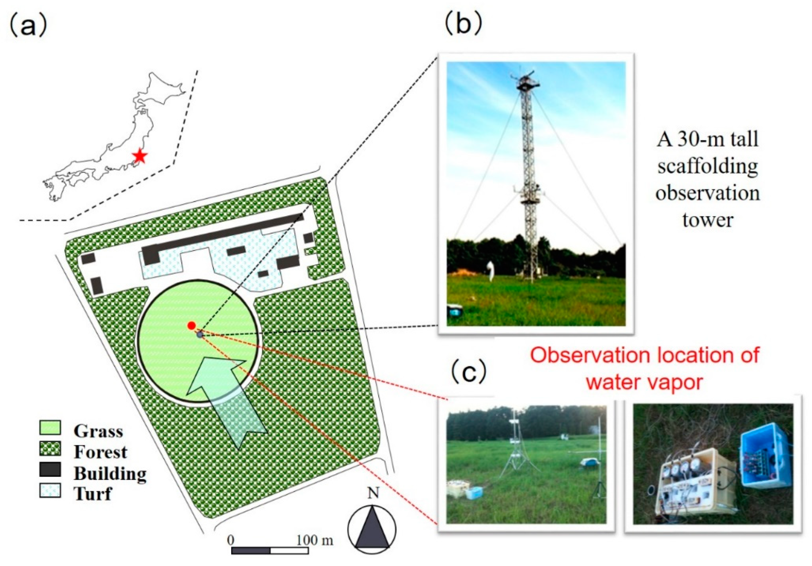
We conducted this study at the experimental fields of the Center for Research in Isotopes and Environmental Dynamics (CRiED) at the University of Tsukuba, Japan (36.1 °N, 140.1 °E), 27 m above sea level (Figure 1a). The mean annual air temperature between 1981 and 2005 was approximately 14.1 °C, and the mean annual precipitation was approximately 1159 mm based on observations at the site. Pine stands and lawn surround the flat, circular field, with a diameter of 160 m. In 2010, mowing was performed on day of year (DOY)213–214. The ground surface was covered by litter composed of mown and dead plants from previous years. The top of the fertile volcanic ash is approximately 2 m thick, under which there is a clay layer. Routine micrometeorological (e.g., downward solar radiation, air temperature, relative humidity, wind speed, and soil heat flux) and eddy covariance measurements (sensible heat flux and latent heat flux) were conducted in the experimental fields of the Center for Research in Isotopes and Environmental Dynamics (Figure 1b). The details regarding the instruments and the database were summarized in Table 1 and more information was described in the literature [35]. We collected a database of stable isotope compositions in different water pools during the three experimental days (Figure 1c).
2.2. In Situ Isotopic and Supporting Dataset Measurements
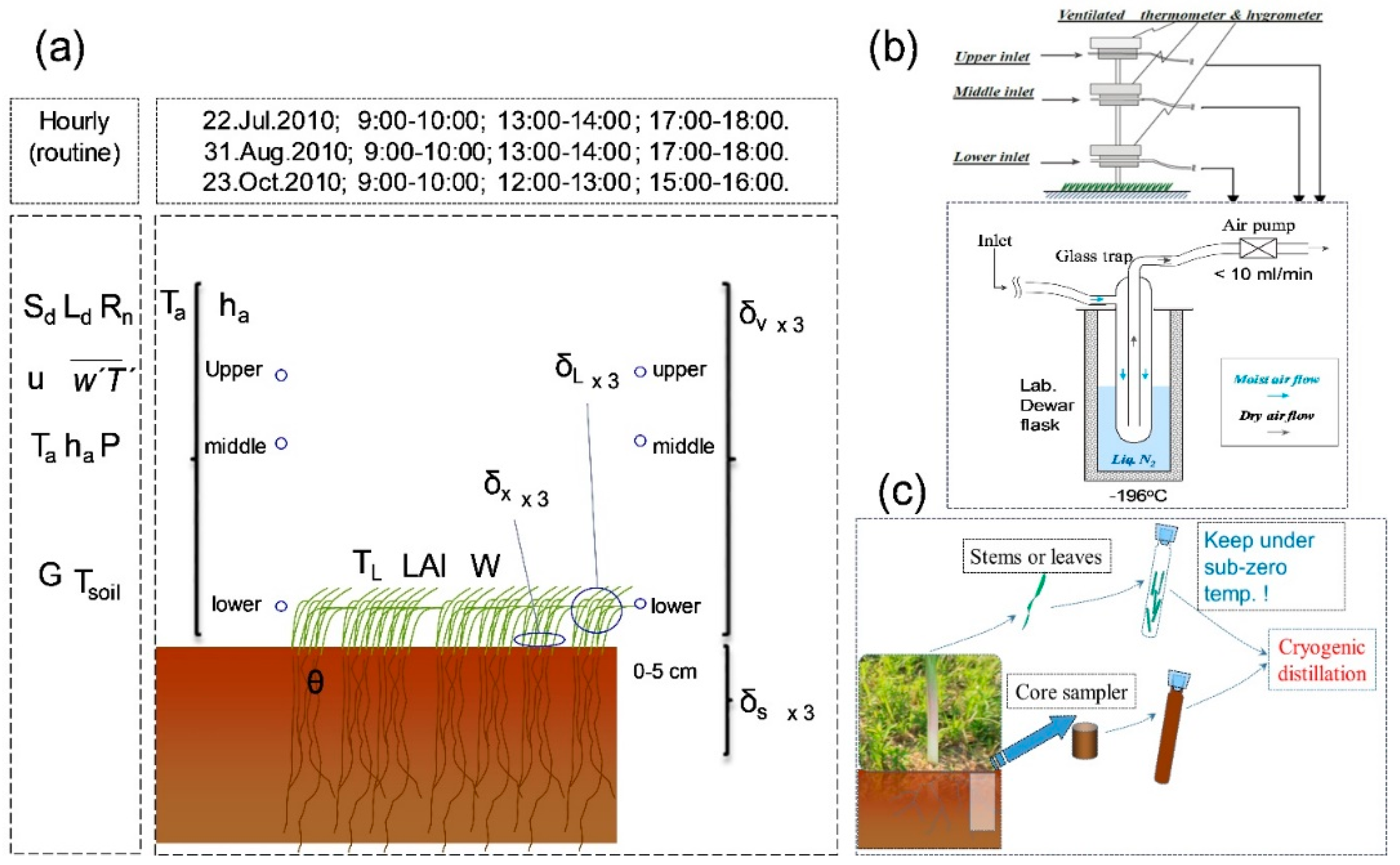
On each day, in the morning (from 09:00 to 10:00 LST), at noon (from 12:00 to 14:00 LST), and in the afternoon (from 15:00 to 18:00 LST), the samples of different water pools (water vapor at three levels, plant stem, plant leaf, and soil) were collected for isotope analysis (Figure 2a). Traditional cold-trap methods were used to collect water vapor for isotopic analysis at the bottom (0.10 m), middle (1.6 m), and upper (2 m) levels (Figure 2b).
Leaf, stem, and soil water samples were collected on a bihourly time interval. For extracting soil water, soil water samples were collected on each sampling day. Leaf and stem water samples were collected from the dominant species, named Miscanthus sinensis, with three replicates. For leaf sampling, the whole leaf was cut and divided into smaller sections and mixed into a test tube. The fresh weight of collected leaves and stems was about 4–5 g. The leaf and stem water samples and surface soil water samples were extracted in the laboratory by a cryogenic distillation method (Figure 2c). At the same time, supporting datasets were also collected. Air temperature and relative humidity were measured at the same level by a ventilated thermometer and a hygrometer for computing the mixing ratio. The leaf water content (W, kg m−2) was measured by weighing the masses of fresh leaves and dry leaves. Leaf area index (LAI) was measured by an automatic area meter by sampling at three spatially different areas following the day after each experiment day. Soil water content in the upper 10 cm of the soil was measured by amplitude domain reflectometry (ADR). The leaf temperature was also measured by a hand-held infrared thermometer during the sampling period. The details of the equipment information are summarized in Table 2. The isotopic ratios of the water samples were analyzed by using a liquid water isotope analyzer (L1102-i, Picarro, Santa Clara, CA, USA), which is a type of wavelength-scanned cavity ring-down spectroscopy, performed at the Center for Research in Isotopes and Environmental Dynamics (CRiED), the University of Tsukuba. The isotopic ratios of 18O and D were expressed as δ18O and δD, respectively, normalized to the Vienna Standard Mean Ocean Water. The analytical errors were 0.1‰ for δ18O and 1‰ for δD [37].
2.3. Iso-SPAC Model
An Iso-SPAC model was used to estimate the water fluxes (E, Ev, and Tr) and their isotopic compositions (δE, δEv, and δTr) [23]. In this model, a SPAC model was used to simulate and partition water and energy fluxes. For the isotope budget, the Craig-Gordon model was used to estimate the δEv. Three sub-models with different complexities, including isotopic steady state (ISS), non-steady-state (NSS), and NSS Péclet models, were tested to determine the actual value for the isotopic composition of plant transpiration (δTr) (Table 3), and the isotopic mass balance equation was used to calculate the δE and was validated by measured values using the Keeling plot approach. The details of this model equations and parameters are described in Appendix A.
2.4. Sensitivity Analysis of Iso-SPAC Model
In order to better understand how the variation in the output of Iso-SPAC model can be attributed to variations of its input factors, the sensitivity analysis was conducted. According to the method proposed by Wang and Yamanaka [16], the sensitivity coefficient (Si) is defined as:
where pi is the i-th interested parameter, and has an effect on the outputs (O), such as E, transpiration fraction (Tr/E), or δTr and δE. Negative Si indicates that a decrease in O results from an increase in pi, and vice versa. The coefficient value of 0.1 means that a 1% increase in pi would induce a 0.1% increase in O. Si provides a measure of the magnitude of O change associated with a unit change of a particular parameter or variable under the condition of a combination of possible ranges and other parameters. The sensitivities of interesting outputs (E, Tr/E, δEv, δTr, and δE) of our study to certain parameters and driving variables are summarized in Table 4. Among those parameters, the minimum leaf stomatal resistance (rst_min) has the greatest influence on changing E; a 30% error in this parameter may result in an error of 8.1% in E on average. Additionally, relative humidity (ha) was the most influential variable in changing E and can produce up to 6.5% error in E if there is 5% error in ha. Such an error range would be a minor problem in practice. For Tr/E, air tempreture (Ta)and LAI were the most influential, although 5% errors in these parameters lead to only 1% and 1.2% errors in Tr/E, respectively. Among many parameters, rst-min is the most influential factor in changing δE; a 30% error in this parameter can introduce a 5.4% error in δE. Additionally, thermal conductivity of surface soil (rss) is the most influential in changing δEv; a 30% error in this parameter can introduce a 3.6% error in δEv. Further, rst-min are influential in changing δTr under NSS; a 30% error in this parameter can introduce a 15.9% error in δTr. Although this possible error range is not always negligible, it is not a serious problem. For measured variables, the isotope composition in water vapor (δV) is the most influential in changing both δE and δEv, which can produce errors of up to 2.95% and 5.35% in δE and δEv, respectively, if there is 5% error in δV. The isotope composition in stem water (δx) is the most influential in changing δTr under both ISS and NSS simulation, and can produce up to 5% error in δTr if there is a 4.5% error in δx under NSS. Such an error range would be a minor problem in practice.
3. Results
3.1. Energy and Water Fluxes
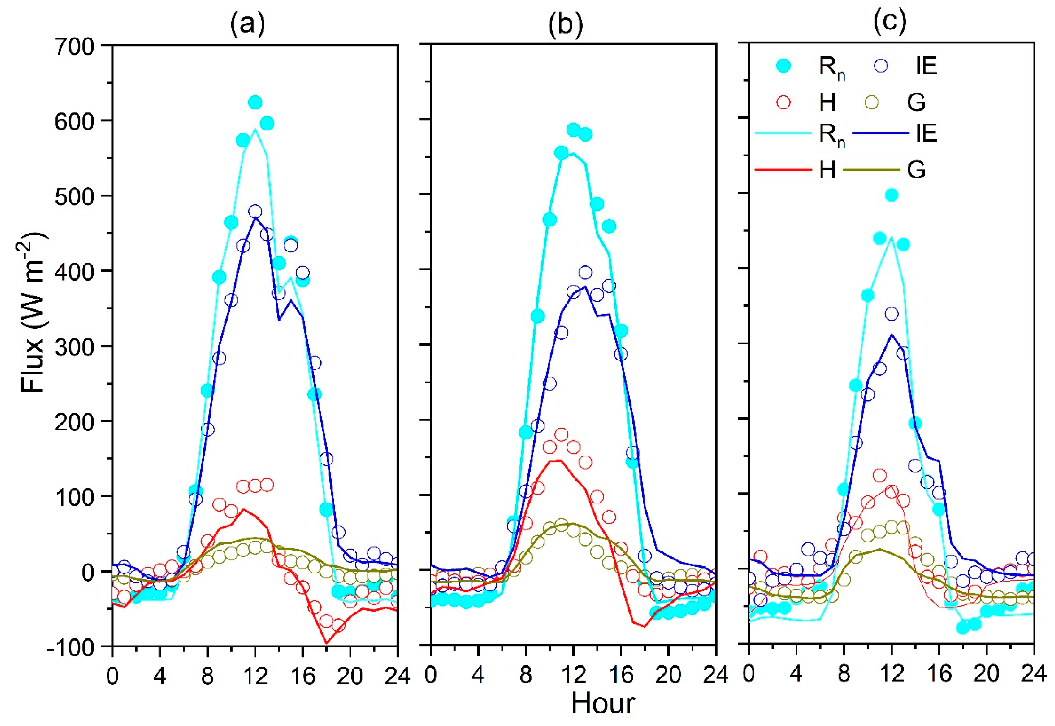
In order to verify the reliability of the model’s simulation of energy fluxes, we compared the observed and simulated values of diurnal variations of all energy fluxes (net radiation, sensible heat, latent heat, and soil heat fluxes) during each experimental day (Figure 3). As summarized in Table 5, the diurnal variation of energy flux was well captured by the Iso-SPAC model. The indices of agreement (I) for the Rn, lE, H, and G simulations were equal to 0.99, 0.98, 0.94, and 0.94, respectively, and the associated RMSD values were 29, 44, 42, and 12.6 W m−2, respectively. The observed and simulated diurnal variation patterns of Rn and lE fluxes were very similar, with respective R2 values of 0.99 and 0.98, during the three experiment days. The peak values for Tr (Ev) that appeared at midday were 0.64 (0.05), 0.41 (0.14), and 0.40 (0.05) mm for DOY 203, 243, and 296, respectively (Figure 4). Moreover, Sensitivity analysis also indicates how the uncertainty in the output of the Iso-SPAC model can be divided and allocated to different sources of uncertainty in its inputs. The value of Si for Tr/E is generally small, suggesting that Tr/E is insensitive to errors in assigned values of all of the parameters.
3.2. Isotope Composition in Water Flux
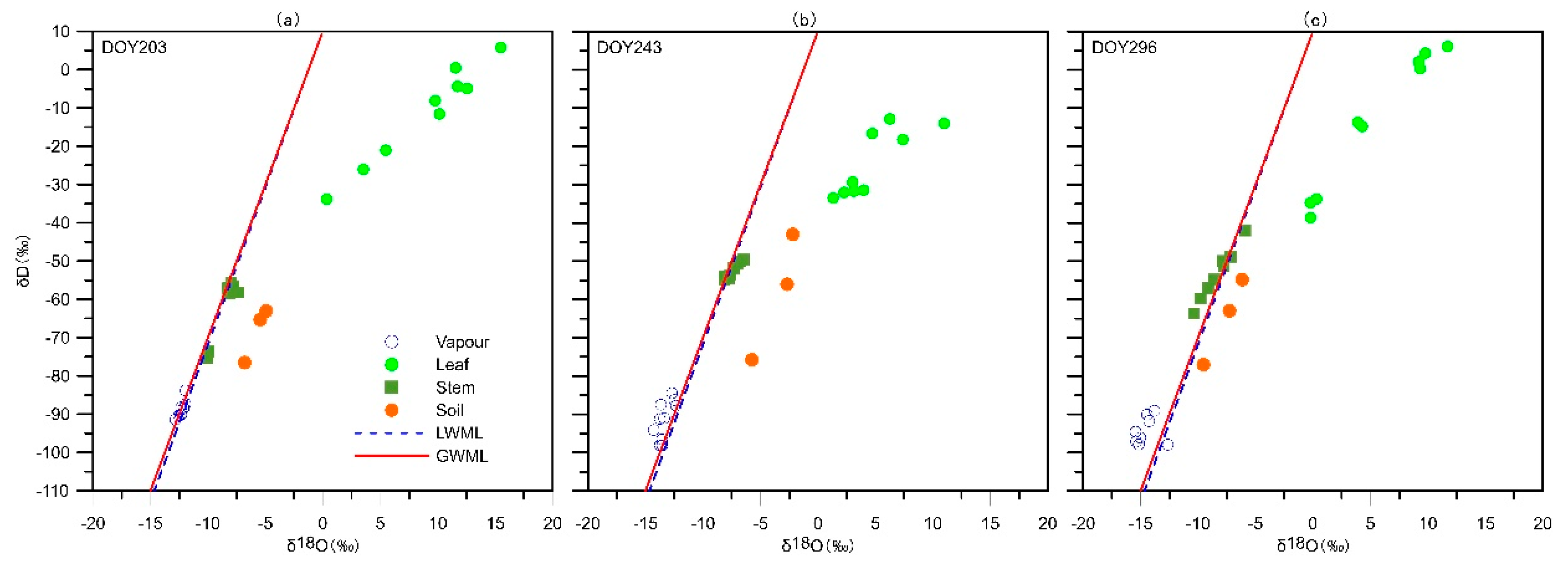
Figure 5 shows a plot between δ18O and δD for all soil, vapor, stem, and leaf water samples for each observation day. The local meteoric water line (LMWL) described by δ2H = 10.2 + 8.2 δ18O [39]. Our measurement results show a consistent pattern of the three observed days. We find that the isotopic composition of surface soil and leaf water deviated from LMWL, which implied that the isotopic kinetic fractionation process at the interface was caused by soil evaporation and plant transpiration. The stem water mainly lies within the LMWL, indicating that the plant water use origin was from precipitation. The isotopic composition of water vapor lies within or slightly deviated from the LMWL, suggesting a departure caused by local recycling effects. Based on the dataset of δV at three levels, the Keeling plot approach, which was used to estimate the δE at each experimental period, is summarized in Table 6. In the daytime (from 08:00 to 18:00 LST), the modeled δE seems to be controlled by LAI. Specifically, the average δE signatures based on the Keeling plot are −9.68‰ when LAI was 2.1 on DOY 203, −16.02‰ when LAI was 0.9 on DOY 243, and −12.17‰ when LAI was 1.5 at DOY 296. This may be because the transpiration fraction is higher when LAI is greater, inducing a high δE [40].
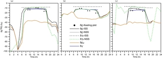
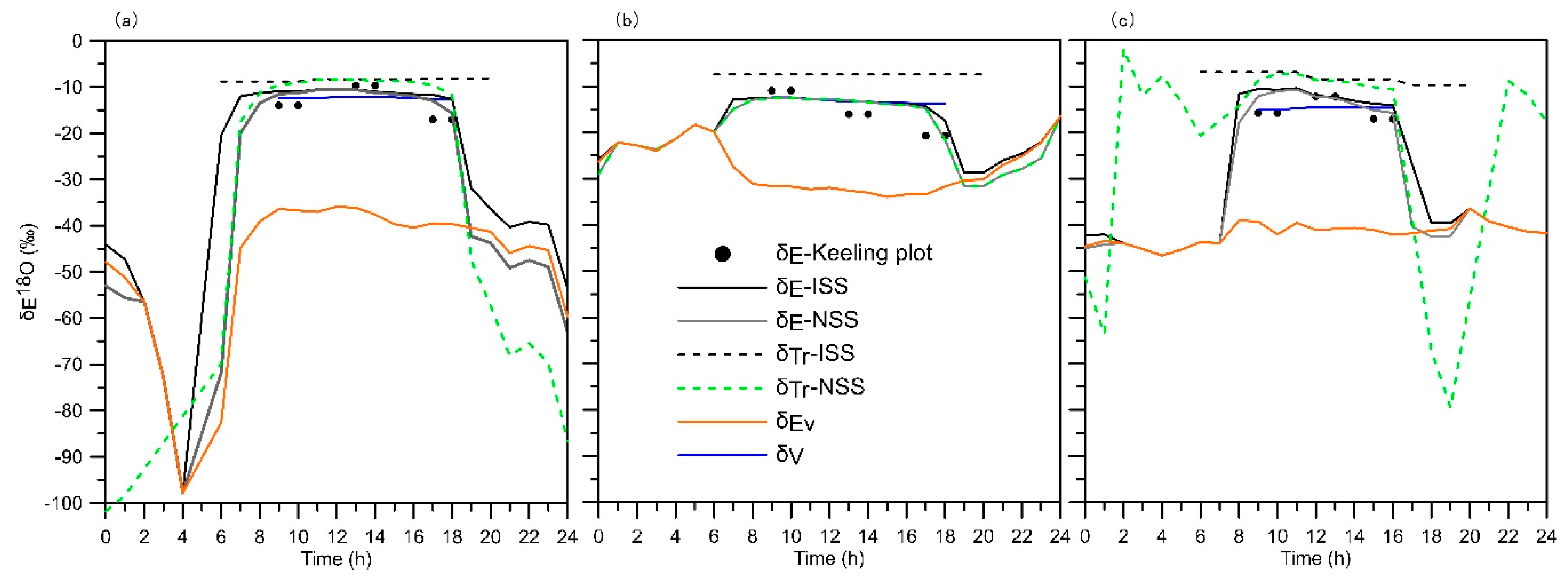
As shown in Figure 6, the temporal variations were reproduced reasonably by all three sub-models for both days with strongly diurnal variations (i.e., DOY 203, DOY 296), as well as days with less variation (DOY 243). The statistics summary of the performances of the three sub-models is shown in Table 7, produced by comparing simulated δE with that of the derived Keeling plot. It is clear that NSS and NSS Péclet can capture the observed diurnal variations better than ISS, while NSS Péclet has few effects on improving the simulation of δE compared to NSS.
3.3. Transpiration Fraction
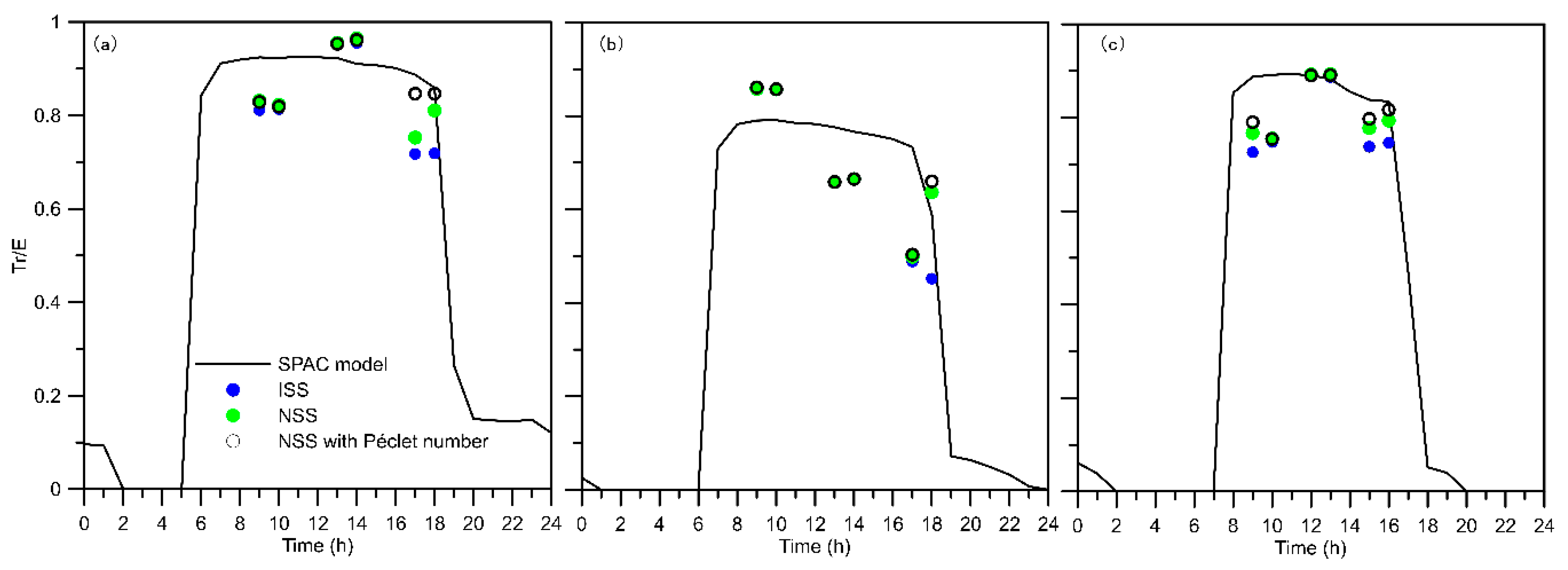
Figure 7 shows the diurnal variations in transpiration fraction (Tr/E) calculated by Tr and E from the Iso-SPAC model, Tr/E estimated by the stable isotope method using δE from the Keeling plot approach, and δEv and δTr from the Iso-SPAC model. Tr/E from Iso-SPAC showed similar diurnal patterns among all three days. Moreover, the value of Si for Tr/E is generally small, suggesting that Tr/E is insensitive to errors in assigned values of all of the parameters. Additionally, day-to-day results show that higher contributions from transpiration from 09:00 to 17:00 LST are found when LAI is higher. Specifically, the mean (standard deviation) values of Tr/E are 0.91 (0.02), 0.70 (0.05), and 0.86 (0.03), with respective LAI of 2.1, 0.9, and 1.5. A lower fraction of less than 0.2 (close to 0) is found during nighttime for all three days. In the three sub-models, the diurnal variation of Tr/E was reasonably captured by the NSS and NSS Péclet. Differences between the isotope method and the Iso-SPAC model vary from 1% to 13%m with an average value of 7.6%. A previous report [41] on the differences between the isotope method and lysimeter plus sap flow measurements range from 4% to 26%, with an average of 15.6%. Considering the uncertainties in isotope measurements, the reasonable agreement between these two methods demonstrates the reliability of the present partitioning results.
3.4. Diurnal Controls of Transpiration Fraction
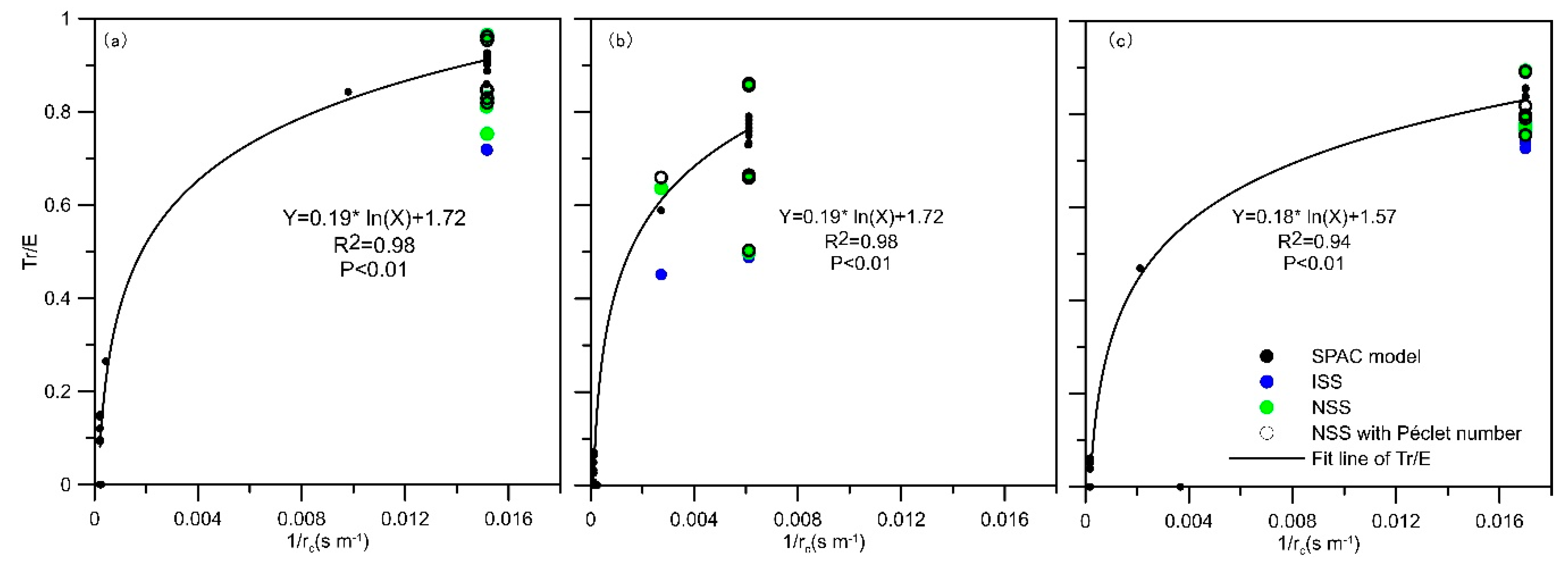
Figure 8 shows the relationship between hourly Tr/E and canopy conductance (=1/rc) over the three days. The Tr/E estimated by isotope approach was limited by rough time resolution and lacking the dataset during the night-time, therefore, the diurnal time series of Tr/E by SPAC model were analyzed. Since the LAI and θ were assumed to be constant within a given day in the present model, the diurnal variation in rC is controlled solely by the downward shortwave radiation (Sd). On the other hand, Figure 6b clarifies the day-to-day variation in the relationship between Tr/E and that the conductance is smaller if we consider the seasonal change in LAI. Nevertheless, the seasonal variation in Tr/E can be well represented as a function of LAI [16,42,43]. This may indicate that LAI regulates seasonal variation in Tr/E, not only via canopy stomata resistance but also via the distribution of radiation energy.
4. Discussion
4.1. Diurnal Water Flux Partitioning
Partition flux can be realized by many approaches, such as the isotopic method and the SPAC model. Previous studies have shown that ISS is better than NSS for describing δTr and isotope composition of leaf water (δL,b) during the entire growing season (Table 8). In our study, more attention was focused on diurnal variations in δE and its components (δTr and δEv). It is worth mentioning that compared with the fixed constant input of δX in the Iso-SPAC model, the use of δX with daily variations (2h interval) can obtain better simulation results of δE. Although similar partitioning results were obtained by ISS, NSS, and NSS Péclet, the performance of ISS was lower than those of NSS and NSS Péclet. Additionally, δTr values simulated by ISS, NSS, and NSS Péclet at midday are close to the ISS assumption (i.e., δTr = δX), suggesting that ISS is reasonable at midday [44]. On the other hand, larger discrepancies between the simulated δTr and ISS and NSS or NSS Péclet were detected for both the periods in the morning and afternoon, when environmental conditions such as solar radiation and stomatal conductance change rapidly. The difference in Tr/E among the four sub-models indicates that there are still many uncertainties regarding the partitioning of E when using the isotope method in the diurnal timescale. These results indicate that for morning or afternoon, NSS is essential for simulating diurnal variations in δTr and δE, because of the relatively rapid changes in environmental conditions. The comparison also shows little improvement of NSS Péclet (which further considers advection-diffusion) in δTr and δE simulation compared to NSS. Nevertheless, non-steady-state behavior should be considered for δTr simulation.
4.2. Isotopic Insights of Water Flux Dynamics into Atmospheric Moisture and Implications
Figure 6 shows the diurnal variations of in situ measured isotopic compositions of atmospheric water vapor (δV) and estimated isotopic compositions of evapotranspiration by the Keeling plot approach (δE–Keeling plot, as well as the simulated isotopic compositions of soil evaporation (δEv), isotopic compositions of transpiration under the state-state assumption (δTr–ISS) and non-steady-state assumption (δTr–NSS), and the simulated isotopic composition of evapotranspiration under ISS (δE–ISS) and NSS (δE–NSS) scenarios. The δV has smaller diurnal variations because of rapid mixing with a larger background vapor pool. Soil evaporation has a depleted isotope signature because of the larger soil water pool. Transpiration shows an enriched isotope signature during the daytime because of fast transpiration flux with a rapid turnover time (less than 1 h) for the leaf water pool, whereas there is a larger deviation at night with a more considerable turnover time (more than 100 h). The pattern of δTr in the night varied day-by-day. At night-time, transpiration flux was much smaller (close to zero), and the leaf water content (W) was almost constant with lower sensitivity for the changes in δTr. The changes of δTr in the night was dynamic and mainly constrained by the night air temperature, relative humidity, leaf water enrichment during the daytime, and δV of the background. The lowest temperature in the night-time was for DOY 296 with the smallest night-time transpiration, which resulted in drastic changes of δTr compared to others (Figure 4 and Figure 6). The isotopic composition in the evapotranspiration flux was a mixture between the isofluxes of soil evaporation and plant transpiration. During the day, the isotope composition in the evapotranspiration flux was mainly controlled by the enriched isoflux of plant transpiration. During the night period, the variations in δE were more complex, and it seemed that the δE was mainly dominated by isoflux of soil evaporation, but there was a mixture both of isoflux from soil evaporation and transpiration after sunset. During the day, transpiration and evaporation, respectively, acted to increase and decrease the δ18O of water vapor, which was affected by the diurnal trade-off between them. At night, the situation was complex, where soil evaporation always acted to deplete the δ18O of water vapor and transpiration varied day-to-day. Clearly, the results indicate that for morning or afternoon, NSS should be considered because of relatively rapid changes in environmental conditions during the period of the day alternating with the night. High-frequency measurements in micrometeorology, fluxes and isotopic compositions in water vapor, even in transpiration, using bulk leaf water to simulate and constrain the diurnal variations in water fluxes, specifically for night-time, is promising.
5. Conclusions
The Iso-SPAC model was applied to simulate the diurnal variations in energy fluxes and isotopic compositions in E. Energy flux estimated by the Iso-SPAC model agreed very well with observed values. Isotopic compositions in E estimated by the Iso-SPAC model with NSS agreed well with those observed by the Keeling plot approach, while ISS is also applicable for times around midday. The Iso-SPAC model is a useful tool to partition E on a diurnal scale. The Tr/E is higher in the daytime and close to 0 at night. The isotopic method based on the Keeling plot approach is also a useful tool. To accurately capture the diurnal variations, the non-steady-state model is required for estimating δTr. The principal factor controlling the diurnal variation of Tr/E is stomatal conductance, which is mainly driven by the diurnal variation of solar radiation.
Author Contributions
Conceptualization, P.W.; methodology, P.W.; software, P.W and Y.D.; validation, P.W.; formal analysis, P.W. and Y.D; investigation, P.W.; resources, P.W.; data curation, P.W.; writing—original draft preparation, P.W. and Z.W; writing—review and editing, P.W. and Z.W; visualization, P.W.; supervision, P.W.; project administration, P.W.; funding acquisition, P.W.
Funding
This research was funded by the Strategic Priority Research Program of the Chinese Academy of Sciences, grant number XDA20100102, the National Natural Science Foundation of China, grant numbers 41730854 and 41671019, and “The projects by the State Key Laboratory of Earth Surface Processes and Resource Ecology”.
Conflicts of Interest
The authors declare no conflict of interest.
Appendix A
The Iso-SPAC model was originally used for the partitioning of energy and water fluxes coupled with the isotopic fractionation process into canopy and soil components at daily time-scales [23].
Appendix A.1. Parameterization of Heat and Water Fluxes and Partitioning of Energy/Water Flux
A soil-plant-atmosphere continuum (SPAC) model of Wang and Yamanaka [16] was adopted here to simulate the daily heat and water fluxes from the canopy and soil layer. The model was selected for several reasons. This model treats the radiation/energy balance properly in both the vegetative canopy and at the ground surface with interactions between them, enabling us to estimate all energy balance components, including the latent heat flux (lE) and its components (lEv and lTr). By assuming that the energy of photosynthesis and that introduced by advection are negligible, equations for the radiation/energy balance in the vegetation canopy and at the ground surface are, respectively, expressed as follows:
where RnV is the net radiation of the vegetation canopy (W m advection−2), HV is the sensible heat flux from the vegetation canopy (W m−2), Tr is the transpiration flux (kg m−2 s−1), fv is the permittivity of the vegetation canopy, αV is the albedo of the vegetation canopy, Sd is the downward shortwave radiation (W m−2), Ld is the downward longwave radiation (W m−2), σ is the Stefan-Boltzmann constant (=5.67 × 10⁻⁸ W m−2 K−4), TG is the ground surface temperature (°C), TL is the leaf temperature (°C), RnG is the net radiation at the ground surface (W m−2), G is the ground heat flux (W m−2), HG is the sensible heat flux from the ground surface (W m−2), Ev is the evaporation flux (kg m−2 s−1), and αG is the albedo of the ground surface. Note that this model is not a patch model but is rather a layer model, and therefore, total flux per unit area is given as the sum of the vegetation canopy and ground surface components; that is, Rn = RnV + RnG, H = HV + HG, and lE = l(Ev + Tr). Second, there is no need for radiometric temperature observations, as the model is separately solved by the Newton-Raphson scheme for vegetation canopy (TL) and ground temperature (TG), which can be easily integrated into the isotopic fractionation processes with H2O exchange in terrestrial ecosystems and has the advantage of enabling the long-term assessment of E partitioning, as well as isotopic enrichment output at the plant–atmosphere interface. Third, this model considers the nonlinear response of plant physiology to light penetration inside the canopy and ground surface by considering the interaction between them. Also, stomatal control of transpiration, including its dependence on soil moisture, is explicitly considered in the model, while some previous models do not consider it. More details are provided by Wang and Yamanaka [16].
Appendix A.2. Three Sub-Models for the Estimation of δTr
Understanding the isotope ratios in leaf water is essential for isotope-flux analyses. The isotope composition at the evaporative site in leaf (δL,e) is needed to estimate δTr, but δL,e cannot be measured directly. Fortunately, we can measure the isotopic composition of bulk leaf water (δL,b) in situ, which can be used for Iso-SPAC model validation. Therefore, the δL,e is a crucial bridge, not only for estimating δTr, but also for δL,b as a first-order approximation. There are many models [29,31,32,33] that have been successful in simulating δL,e or δL,b at the leaf scale. In this study, three existing leaf water isotope enrichment sub-models were used to estimate δL,e, δTr, and δL,b at the canopy scale. Detailed descriptions of each model are provided below.
Appendix A.3. Model 1: Isotopic Steady-State (ISS)
Under the isotopic steady-state assumption (ISS), the water that exits the leaf has the same isotopic composition as xylem water, so we can substitute δX for δTr to revise the Craig and Gordon (C&G)model, such that the isotopic composition of leaf water at the evaporation site δL,e under ISS can be estimated by the following equation [31],
where δL,es is the δ of leaf water at the evaporating site under ISS, and δV, and δX are the δ values of xylem water and atmospheric water vapor, respectively. Additionally, ε+ and h* are the equilibrium fractionation factor and relative humidity of the ambient air reference to the leaf temperature, respectively, and εk is the canopy kinetic fractionation factor given as
where ra, rb and rc are the aerodynamic, boundary-layer, and canopy resistances, respectively;
rc is given as:
where rst is the leaf stomatal resistance. While many types of the rst parameterization have been proposed, the following equation was applied in the present study:
where rst_min and rst_max are the minimum and maximum values, respectively, of leaf stomatal resistance (s m−1) when the soil is sufficiently wet. We set rst_min = 100 and rst_max = 10,000 by the trial and error method to minimize the difference between predicted and measured energy fluxes. Similarly, the empirical parameters were determined as follows: csw = θ/θmax (for which θ is the volumetric soil water content (m3 m−3), θmax (= 0.45 m3 m−3) is the maximum water content in the study period), and csd = 25 (W m−2).
To estimate the rb, we assume that the wind speed inside the canopy takes the usual exponential form controlled by LAI.
The mean wind speed inside the canopy (uc) is given as
where uv is the wind speed at the vegetation height, which is estimated by the following equation:
where zV is the vegetation height (m), zm is the height of wind speed measurement (m), d0 (=0.666zV) is the zero-plane displacement height (m), z0mV (=0.123zV) is the roughness length governing momentum transfer above vegetation canopy (m), and u is the wind speed (m s−1).
Additionally, rb, scaled to the canopy, is calculated using the following equation
where Lw is the leaf dimension (=0.01 m).
The ra in the surface layer is not isotopically discriminating and can be computed as the difference between rav and rb:
Here, raV can be determined as follows:
where zh is the height of temperature and humidity measurements (m), z0hV (=0.1z0mV) is the roughness length governing heat (and vapor) transfer above the vegetation canopy (m), and k is the von Karman’s constant (=0.41).
Appendix A.4. Model 2: Non Steady State (NSS)
The non-steady state model, which considers a departure from the steady-state condition, was used to predict δL,e [31] as follows:
where δL,e is the δ18O or δD value of leaf water at the evaporation site, and the superscript o denotes the initial value of δL,e at time zero. The time constant τ is given as
where W is the leaf water content (kg m−2), rt is the leaf total (i.e., including stomata and boundary layer in series) resistance (s m−1), wi is the water vapor concentration saturated at leaf temperature (mol mol−1), and t represents time (s).
The δTr was estimated by considering the departure from ISS using δL,e as follows:
where h* is the relative humidity normalized by the leaf temperature.
Appendix A.5. Nonsteady State (NSS) with Péclet Model
Model 3 [29] simultaneously considers the NSS effects and Péclet effect to predict δL,e and δTr as follows:
where δTr was estimated by considering the departure from ISS using δL,e, as follows:
where h* is the relative humidity normalized by the leaf temperature.
Appendix A.6. Estimation of δEv
The calculation of δEv based on the Craig and Gordon model [38]
where δe represents the δ18O or δD value of soil water at the evaporation front, δV is the δ18O or δD values of the background atmospheric water vapor, α+ (>1) is the temperature-dependent equilibrium fractionation factor between liquid and vapor, ε+ = 1000(1 − 1/α+), εk is the isotopic kinetic fractionation associated with diffusion of water through the soil, and h* is relative humidity normalized by the soil temperature (TG) at the evaporation front.
Appendix A.7. Estimation of δE
An isotopic mass balance equation was used to estimate δE. The E is composed of Ev and Tr, such that
where each flux is characterized by the isotopic signatures δE, δEv, and δTr.
The isotopic mass balance can be expressed by
The isotope composition in the E flux can be calculated using EvδEv and the corresponding transpiration isoflux (e.g., TrδTr under ISS or NSS).
References
- Yakir, D.; Wang, X.F. Fluxes of CO2 and water between terrestrial vegetation and the atmosphere estimated from isotope measurements. Nature 1996, 380, 515–517. [Google Scholar] [CrossRef]
- Yepez, E.A.; Williams, D.G.; Scott, R.L.; Lin, G. Partitioning overstory and understory evapotranspiration in a semiarid savanna woodland from the isotopic composition of water vapor. Agric. Meteorol. 2003, 119, 53–68. [Google Scholar] [CrossRef]
- Good, S.P.; Noone, D.; Bowen, G. Hydrologic connectivity constrains partitioning of global terrestrial water fluxes. Science 2015, 349, 175. [Google Scholar] [CrossRef] [PubMed]
- Katul, G.G.; Oren, R.; Manzoni, S.; Higgins, C.; Parlange, M.B. Evapotranspiration: A process driving mass transport and energy exchange in the soil–plant–atmosphere–climate system. Rev. Geophys. 2012, 50, 1209–8755. [Google Scholar] [CrossRef]
- Wang, P.; Deng, Y.; Li, X.-Y.; Wei, Z.; Hu, X.; Tian, F.; Wu, X.; Huang, Y.; Ma, Y.-J.; Zhang, C.; et al. Dynamical effects of plastic mulch on evapotranspiration partition in a mulched agriculture ecosystem: Measurement with numerical modeling. Agric. Meteorol. 2019, 268, 98–108. [Google Scholar] [CrossRef]
- Williams, D.G.; Cable, W.; Hultine, K.; Hoedjes, J.C.B.; Yepez, E.A.; Simonneaux, V.; Er-Raki, S.; Boulet, G.; de Bruin, H.A.R.; Chehbouni, A.; et al. Components of evapotranspiration in an olive orchard determined by eddy covariance, sap flow and stable isotope techniques. Agric. Meteorol. 2004, 125, 241–258. [Google Scholar] [CrossRef]
- Aouad, G.; Ezzahar, J.; Amenzou, N.; Er-Raki, S.; Benkaddour, A.; Khabba, S.; Jarlan, L. Combining stable isotopes and micrometeorological measurements for partitioning evapotranspiration of winter wheat into soil evaporation and plant transpiration in a semi-arid region. Agric. Water Manag. 2016, 177, 181–192. [Google Scholar] [CrossRef]
- Jelka, B.; Christian, M.; Alexander, K. Eddy covariance measurements of the dual-isotope composition of evapotranspiration. Agric. Meteorol. 2019, 269, 203–219. [Google Scholar]
- Maria, Q.; Anne, K.; Alexander, G.; Nicolas, B.; Youri, R. In-situ monitoring of soil water isotopic composition for partitioning of evapotranspiration during one growing season of sugar beet (Beta vulgaris). Agric. Meteorol. 2019, 266, 53–64. [Google Scholar]
- Wei, Z.; Yoshimura, K.; Okazaki, A.; Ono, K.; Kim, W.; Yokoi, M.; Lai, C.T. Understanding the variability of water isotopologues in near-surface atmospheric moisture over a humid subtropical rice paddy in Tsukuba, Japan. J. Hydrol. 2016, 533, 91–102. [Google Scholar] [CrossRef] [Green Version]
- Zhao, L.; Liu, X.; Wang, N.; Kong, Y.; Song, Y.; He, Z.; Liu, Q.; Wang, L. Contribution of recycled moisture to local precipitation in the inland Heihe River Basin. Agric. Meteorol. 2019, 271, 316–335. [Google Scholar] [CrossRef]
- Penna, D.; Hopp, L.; Scandellari, F.; Allen, S.T.; Benettin, P.; Beyer, M.; Geris, J.; Klaus, J.; Marshall, J.D.; Schwendenmann, L.; et al. Ideas and perspectives: Tracing terrestrial ecosystem water fluxes using hydrogen and oxygen stable isotopes–challenges and opportunities from an interdisciplinary perspective. Biogeosciences 2018, 15, 6399–6415. [Google Scholar] [CrossRef]
- Griffis, T.J. Tracing the flow of carbon dioxide and water vapor between thebiosphere and atmosphere: A review of optical isotope techniques and their application. Agric. Meteorol. 2013, 174, 85–109. [Google Scholar] [CrossRef]
- Ménard, C.B.; Ikonen, J.; Rautiainen, K.; Aurela, M.; Arslan, A.N.; Pulliainen, J. Effects of Meteorological and Ancillary Data, Temporal Averaging, and Evaluation Methods on Model Performance and Uncertainty in a Land Surface Model. J. Hydrometeorol. 2015, 16, 2559–2576. [Google Scholar] [CrossRef]
- Shuttleworth, W.J.; Wallace, J. Evaporation from sparse crops–an energy combination theory. Q. J. R. Meteorol. Soc. 1985, 111, 839–855. [Google Scholar] [CrossRef]
- Wang, P.; Yamanaka, T. Application of a two-source model for partitioning evapotranspiration and assessing its controls in temperate grasslands in central Japan. Ecohydrology 2014, 7, 345–353. [Google Scholar] [CrossRef]
- Norman, J.M.; Anderson, M.C.; Kustas, W.P.; French, A.N.; Mecikalski, J.; Torn, R.; Diak, G.R.; Schmugge, T.J.; Tanner, B.C.W. Remote sensing of surface energy fluxes at 101-m pixel resolutions. Water Resour. Res. 2003, 39, 1221. [Google Scholar] [CrossRef]
- Norman, J.M.; Becker, F. Terminology in thermal infrared remote sensing of natural surfaces. Agric. Meteorol. 1995, 77, 153–166. [Google Scholar] [CrossRef]
- Anderson, M.C.; Norman, J.M.; Mecikalski, J.R.; Torn, R.D.; Kustas, W.P.; Basara, J.B. A multiscale remote sensing model for disaggregating regional fluxes to micrometeorological scales. J. Hydrometeorol. 2004, 5, 343–363. [Google Scholar] [CrossRef]
- Braud, I.; Dantas-Antonino, A.; Vauclin, M.; Thony, J.; Ruelle, P. A simple soil-plant-atmosphere transfer model (SiSPAT) development and field verification. J. Hydrol. 1995, 166, 213–250. [Google Scholar] [CrossRef]
- Braud, I.; Bariac, T.; Gaudet, J.P.; Vauclin, M. SiSPAT-Isotope, a coupled heat, water and stable isotope (HDO and H218O) transport model for bare soil. Part, I. Model description and first verifications. J. Hydrol. 2005, 309, 277–300. [Google Scholar] [CrossRef]
- Braud, I.; Bariac, Z.; Vauclin, M.; Boujamlaoui, Z.; Gaudet, J.; Biron, P.; Richard, P. SiSPAT-Isotope, a coupled heat, water and stable isotope (HDO and H218O) transport model for bare soil. Part II. Evaluation and sensitivity tests using two laboratory data sets. J. Hydrol. 2005, 309, 301–320. [Google Scholar] [CrossRef]
- Wang, P.; Yamanaka, T.; Li, X.-Y.; Wei, Z. Partitioning evapotranspiration in a temperate grassland ecosystem: Numerical modeling with isotopic tracers. Agric. Meteorol. 2015, 208, 16–31. [Google Scholar] [CrossRef]
- Wang, P.; Li, X.Y.; Huang, Y.; Liu, S.; Xu, Z.; Wu, X.; Ma, Y. Numerical modeling the isotopic composition of evapotranspiration in an arid artificial oasis cropland ecosystem with high–frequency water vapor isotope measurement. Agric. Meteorol. 2016, 230, 79–88. [Google Scholar] [CrossRef]
- Wei, Z.; Lee, X.; Wen, X.; Xiao, W. Evapotranspiration partitioning for three agro-ecosystems with contrasting moisture conditions: A comparison of an isotope method and a two-source model calculation. Agric. Meteorol. 2018, 252, 296–310. [Google Scholar] [CrossRef]
- Wei, Z.; Yoshimura, K.; Okazaki, A.; Kim, W.; Liu, Z.; Yokoi, M. Partitioning of evapotranspiration using high-frequency water vapor isotopic measurement over a rice paddy field. Water Resour. Res. 2015, 51, 3716–3729. [Google Scholar] [CrossRef]
- Riley, W.; Still, C.; Torn, M.; Berry, J. A mechanistic model of H218O and C18OO fluxes between ecosystems and the atmosphere: Model description and sensitivity analyses. Glob. Biogeochem. Cycles 2002, 16, 1095. [Google Scholar] [CrossRef]
- Lai, C.T.; Ehleringer, J.R.; Bond, B.J.; Paw, U.K.T. Contributions of evaporation, isotopic non-steady state transpiration and atmospheric mixing on the δ18O of water vapor in Pacific Northwest coniferous forests. Plant Cell Environ. 2005, 29, 77–94. [Google Scholar] [CrossRef]
- Farquhar, G.D.; Cernusak, L.A. On the isotopic composition of leaf water in the non-steady state. Funct. Plant Biol. 2005, 32, 293–303. [Google Scholar] [CrossRef] [Green Version]
- Dubbert, M.; Cuntz, M.; Piayda, A.; Werner, C. Oxygen isotope signatures of transpired water vapor: The role of isotopic non-steady-state transpiration under natural conditions. New Phytol. 2014, 203, 1242–1252. [Google Scholar] [CrossRef]
- Dongmann, G.; Nürnberg, H.W.; Förstel, H.; Wagener, K. On the enrichment of H218O in the leaves of transpiring plants. Radiat. Environ. Biophys. 1974, 11, 41–52. [Google Scholar] [CrossRef] [PubMed]
- Ogée, J.; Cuntz, M.; Peylin, P.; Bariac, T. Non-steady-state, non-uniform transpiration rate and leaf anatomy effects on the progressive stable isotope enrichment of leaf water along monocot leaves. Plant Cell Environ. 2007, 30, 367–387. [Google Scholar] [CrossRef] [PubMed]
- Cuntz, M.; Ogee, J.; Farquhar, G.D.; Peylin, P.; Cernusak, L.A. Modelling advection and diffusion of water isotopologues in leaves. Plant Cell Environ. 2007, 30, 892–909. [Google Scholar] [CrossRef] [PubMed]
- Dubbert, M.; Werner, C. Water fluxes mediated by vegetation: Emerging isotopic insights at the soil and atmosphere interfaces. New Phytol. 2019, 221, 1754–1763. [Google Scholar] [CrossRef] [PubMed]
- Ma, W.; Asanuma, J.; Xu, J.; Onda, Y. A database of water and heat observations over grassland in the north-east of Japan. Earth Syst. Sci. Data 2018, 10, 2295–2309. [Google Scholar] [CrossRef] [Green Version]
- Yamanaka, T.; Tsunakawa, A. Isotopic signature of evapotranspiration flux and its use for partitioning evaporation/transpiration components. Tsukuba Geoenviron. Sci. 2007, 3, 11–21. [Google Scholar]
- Yamanaka, T.; Onda, Y. On measurement accuracy of liquid water isotope analyzer based on wavelength-scanned cavity ring-down spectroscopy (WS-CRDS). Bull. Terr. Environ. Res. Cent. Univ. Tsukuba 2011, 12, 31–40. [Google Scholar]
- Craig, H.; Gordon, L.I. Deuterium and oxygen-18 variations in the ocean and the marine atmosphere. In Stable Isotopes in Oceanographic Studies and Palaiotemperatures; Tongiorgi, E., Ed.; Lab. Geol. Nucl.: Pisa, Italy, 1965; pp. 1–122. [Google Scholar]
- Yabusaki, S.; Tase, N. Formation Process of vertical profile of stable isotopes in soil water at TERC. Bull. Terr. Environ. Res. Cent. Univ. Tsukuba 2007, 8, 17–26. [Google Scholar]
- Breshears, D.D. The grassland-forest continuum: Trends in ecosystem properties for woody plant mosaics? Front. Ecol. Environ. 2006, 4, 96–104. [Google Scholar] [CrossRef]
- Wang, L.; Caylor, K.K.; Villegas, J.C.; Barron-Gafford, G.A.; Breshears, D.D.; Huxman, T.E. Partitioning evapotranspiration across gradients of woody plantcover: Assessment of a stable isotope technique. Geophys. Res. Lett. 2010, 37, L09401. [Google Scholar] [CrossRef]
- Tong, Y.; Wang, P.; Li, X.-Y.; Wang, L.; Wu, X.; Shi, F.; Bai, Y.; Li, E.; Wang, J.; Wang, Y. Seasonality of the transpiration fraction and its controls across typical ecosystems within the Heihe River Basin. J. Geophys. Res. Atmos. 2019, 124, 1277–1291. [Google Scholar] [CrossRef]
- Wang, P.; Li, X.Y.; Wang, L.X.; Wu, X.C.; Hu, X.; Fan, Y.; Tong, Y.Q. Divergent evapotranspiration partition dynamics between shrubs and grasses in a shrub-encroached steppe ecosystem. New Phytol. 2018, 219, 1325–1337. [Google Scholar] [CrossRef] [PubMed]
- Welp, L.R.; Lee, X.; Kim, K.; Grifronfis, T.J.; Billmark, K.A.; Baker, J.M. δ18O of water vapour, evapotranspiration and the sites of leaf water evaporation in asoybean canopy. Plant Cell Environ. 2008, 31, 1214–1228. [Google Scholar] [CrossRef] [PubMed]
Figure 1.
Experimental field. (a) Panorama of the experimental field during the initial growing period. Block arrows indicate the dominant wind direction in the study site during the growing season. Modified from Yamanaka and Akiyoshi, 2007 [36]. (b) Field photos of a 30-m tall scaffolding observation tower with instrumentation of the eddy correlation system. (c) Photos of field measurements of water vapor.

Figure 2.
(a) Description of the dataset of routine measurements and in situ isotopic samplings. (b) Water vapor sampling system modified from Yamanaka and Akiyoshi, 2007 [36]. (c) Stems, leaves, and soil sampling.
Figure 2.
(a) Description of the dataset of routine measurements and in situ isotopic samplings. (b) Water vapor sampling system modified from Yamanaka and Akiyoshi, 2007 [36]. (c) Stems, leaves, and soil sampling.

Figure 3.
Diurnal variations in the observed (circles) and simulated (lines) energy fluxes (Rn is net radiation, lE is latent heat flux, H is sensible heat flux, G is ground heat flux) during observation periods.
Figure 3.
Diurnal variations in the observed (circles) and simulated (lines) energy fluxes (Rn is net radiation, lE is latent heat flux, H is sensible heat flux, G is ground heat flux) during observation periods.

Figure 4.
Diurnal variations in evapotranspiration (E), plant transpiration (Tr), and soil evaporation (Ev) simulated by the Iso-SPAC model.
Figure 4.
Diurnal variations in evapotranspiration (E), plant transpiration (Tr), and soil evaporation (Ev) simulated by the Iso-SPAC model.

Figure 5.
Plots between stable water isotope of oxygen (δ18O) and hydrogen (δD) in soil-plant-atmosphere continuum (SPAC) for soil, vapor, stem, and leaf water samples for Miscanthus sinensis for each observation day. The blue dash line is the local meteoric water line (LMWL) that is described by δ2H = 10.2 + 8.2 δ18O, provided by Yabusaki and Tase (2007). The red solid line is the Global Meteoric Water Line (GMWL).

Figure 6.
The diurnal variations of in situ measured isotopic compositions of atmospheric water vapor (δV) and estimated isotopic composition of evapotranspiration by the Keeling plot approach (δE–Keeling plot), as well as the simulated isotopic composition of soil evaporation (δEv), the isotopic composition of transpiration under the state–state assumption (δTr–ISS) and non-steady-state assumption (δTr–NSS), as well as the simulated isotopic composition of evapotranspiration under ISS (δE–ISS) and NSS (δE–NSS) scenarios.

Figure 7.
Diurnal variations in transpiration fraction (Tr/E) simulated by the SPAC model and estimated by the Keeling plot approach with three sub modules, including isotopic steady state (ISS), non-steady state (NSS), and NSS Péclet.
Figure 7.
Diurnal variations in transpiration fraction (Tr/E) simulated by the SPAC model and estimated by the Keeling plot approach with three sub modules, including isotopic steady state (ISS), non-steady state (NSS), and NSS Péclet.

Figure 8.
Relationship of canopy conductance (1/rc; rc is the canopy resistance) with transpiration fraction (Tr/E) for each investigation day.
Figure 8.
Relationship of canopy conductance (1/rc; rc is the canopy resistance) with transpiration fraction (Tr/E) for each investigation day.


Table 1.
Summary of routine instrument and information of the dataset.
| Variables | Eddy Correlation System | Height of Measurement (m) |
|---|---|---|
| Net radiation, Rn | (aCN-81, EKO, Tokyo, Japan) | 1.6 |
| Soil heat flux, G | (bCN-11, EKO, Tokyo, Japan) | −0.05 |
| Air temperature, Ta relative humidity, ha | (cCVS-HMP45D, Climatec Inc., Tokyo, Japan) | 1.6 |
| Sensible heat flux, H | (dDA-650, Kaijo, Tokyo, Japan) | 1.6 |
a Type of a net radiometer; b Type of a heat flux plate; c Temperature and relative humidity sensor, Vaisala; d A 3D Ultrasonic wind speed thermometer.
Table 2.
Summary of information of instruments for supporting dataset.
| Variables | Equipment | Measurements |
|---|---|---|
| Air temperature, Ta | Ventilated thermometer, (aPFT-01, PREDE, Japan) | 3 or 4 levels, 5 min interval |
| Air humidity, ha | Ventilated hygrometer, (bCHS-APS, TDK, Japan) | |
| Leaf temperature, TL | Infrared-radiation-thermometer, (cPT-7LD, Optex, Shiga, Japan) | 60 repetition per |
| Leaf area index, LAI | Automatic area meter, (dAAM -7, Hayashi Denko, Japan) | 3 repetitions |
| Leaf water content, W | Gravimetric | 3 repetition |
| Soil water content, θ | Soil moisture meter, (eDIK-311C, Daiki, Japan) | 15 repetition per hour |
a Type of air tempreture sensor; b Type of humidity sensor; c Protable non-contact thermometer; d Automatic area meter, e Type of a soil moisture meter.
Table 3.
Description of three sub-models for the isotopic composition of transpiration flux.
| Sub-Models | Reference | dδTr and eδE | |||
|---|---|---|---|---|---|
| ISS | Péclet Number | W fVariation | NSS | ||
| ISS modela | Craig and Gordon (1965), [38] | Yes | No | No | No |
| NSS modelb | Dongmann et al. (1974), [31] | No | No | No | Yes |
| NSS Pécletc model | Farquhar and Cernusak (2005), [29] | No | Yes | Yes | Yes |
Note: a Isotopic steady-state; b Non-steady state; c Non-steady state with the Péclet number; d Isotope composition in transpiration flux; e Isotope composition in evapotranspiration flux; f Leaf water content per unit area.
Table 4.
Mean of sensitivity coefficients (Si) of modeled mean values of evapotranspiration (E), transpiration fraction (Tr/E), and isotope composition in soil evaporation, transpiration, and evapotranspiration (δEv, δTr, and δE) for O18/O16 under non-steady state (NSS) parameters and driving variables.
| Model Input | uE | vTr/E | wδEv | xδTr | yδE | |
|---|---|---|---|---|---|---|
| Parameters | arst_min | −0.28 | −0.08 | 0.00 | −0.53 | −0.18 |
| brst_max | −0.01 | 0.00 | 0.00 | −0.01 | 0.00 | |
| cαV | −0.17 | −0.02 | 0.00 | −0.03 | −0.04 | |
| dαG | −0.01 | 0.01 | −0.01 | 0.00 | 0.01 | |
| eCLAI | 0.02 | 0.06 | −0.07 | 0.03 | 0.10 | |
| frss | −0.05 | 0.06 | −0.12 | 0.00 | 0.05 | |
| Variables | gSd | 0.72 | 0.00 | 0.07 | 0.21 | 0.10 |
| hLd | 0.84 | −0.03 | 0.17 | 0.33 | 0.03 | |
| iu | 0.08 | 0.00 | −0.17 | 0.19 | −0.05 | |
| jTa | 0.74 | 0.21 | −0.38 | 0.93 | 0.56 | |
| kha | −1.31 | 0.12 | −0.80 | 0.93 | 0.03 | |
| lP | −0.04 | −0.01 | 0.01 | 0.01 | 0.00 | |
| mLAI | 0.42 | 0.26 | −0.06 | 0.55 | 0.13 | |
| nZv | 0.23 | 0.03 | 0.01 | 0.46 | 0.08 | |
| oTsoil | 0.24 | −0.17 | 0.43 | 0.17 | −0.19 | |
| pθ | 0.42 | 0.12 | 0.00 | 0.00 | 0.00 | |
| Isotope budget | qW | N/A | N/A | 0.00 | −0.52 | 0.02 |
| rδV | N/A | N/A | 1.07 | 0.07 | 0.59 | |
| sδS | N/A | N/A | 0.70 | 0:00 | 0.51 | |
| tδX | N/A | N/A | 0.00 | 0.99 | 0.41 | |
Note: a Minimum stomata resistance; b Maximum stomata resistance; c Albedo of vegetation canopy; d Albedo of the ground surface; e Clumping factor for canopy structure; f Thermal conductivity of surface soil; g Downward long-wave radiation; h Downward long-wave radiation; i Wind speed; j Air temperature; k Relative humidity; l Air pressure; m Leaf area index; n Vegetation height; o Soil surface temperature at depth Zsoil; p Volumetric soil water content; q Leaf water content per unit area; r Isotope composition in water vapor; s Isotope composition in soil water; t Isotope composition in stem water, u Evapotranspiration; v Transpiration fraction; w Isotope composition in soil evaporation; x Isotope composition in transpiration flux; y Isotope composition in evapotranspiration flux.
Table 5.
Statistics of the model performance for energy flux and leaf temperature.
| Flux | Unit | fRMSD | gI Index | hR2 | in |
|---|---|---|---|---|---|
| aRn | (W m−2) | 29 | 0.99 | 0.99 | 75 |
| blE | 39 | 0.96 | 0.98 | 75 | |
| cH | 42 | 0.94 | 0.94 | 75 | |
| dG | 12.6 | 0.96 | 0.94 | 75 | |
| eTL | °C | 1.07 | 0.99 | 0.98 | 18 |
Note: a Net radiation; b Latent heat flux; c Sensible heat flux; d Ground heat flux; e Leaf temperature; f Root mean square difference; g Agreement index; h R is correlation coefficient; i Numbers of statistics.
Table 6.
Summary of the Keeling plot method to estimate stable water isotope of oxygen (δ18O) in evapotranspiration flux during three observation days.
Table 6.
Summary of the Keeling plot method to estimate stable water isotope of oxygen (δ18O) in evapotranspiration flux during three observation days.
| aDOY | Time Interval | Linear Equation | bδE (‰) |
|---|---|---|---|
| 203 | 9:00~10:00 | cy = −0.03xd − 14.03 | −14.03 |
| 13:00~14:00 | y = 0.05x − 9.68 | −9.68 | |
| 17:00~18:00 | y = 0.08x − 17.01 | −17.01 | |
| 243 | 9:00~10:00 | y = −0.03x − 10.94 | −10.94 |
| 13:00~14:00 | y = −0.05x − 16.02 | −16.02 | |
| 17:00~18:00 | y = −0.11x − 20.74 | −20.74 | |
| 296 | 9:00~10:00 | y = −0.008x − 15.79 | −15.79 |
| 12:00~13:00 | y = −0.039x − 12.17 | −12.17 | |
| 15:00~16:00 | y = −0.035x − 17.05 | −17.05 |
Note: a day of year; b isotope composition in evapotranspiration flux; c isotope ratios of water vapor; d inverse of specific humidity of water vapor.
Table 7.
Statistics of model performance regarding δ18O in evapotranspiration flux.
| Sub-module | ISSa | NSSb | NSS Pécletc | nd |
|---|---|---|---|---|
| eR2 | 0.43 | 0.52 | 0.51 | 18 |
| fI index | 0.99 | 0.99 | 0.99 | 18 |
| gRMSD ‰ | 3.44 | 2.72 | 2.69 | 18 |
Note: a Isotopic steady-state; b Nonsteady state; c Non-steady-state with the Péclet number; d Number of measurements; e R is correlation coefficient; f Agreement index; g Root mean square difference.
Table 8.
Root mean square difference (RMSD) and agreement index (I) for δ18O between observations and predictions in evapotranspiration (or bulk leaf water).
Table 8.
Root mean square difference (RMSD) and agreement index (I) for δ18O between observations and predictions in evapotranspiration (or bulk leaf water).
| Reference | Ecosystem Type (Location) | Time Scale | aδE | |||
|---|---|---|---|---|---|---|
| bR2 | cRMSD (‰) | dI | en | |||
| Wang et al., 2015 [23] | Temperate grassland (Ibaraki, Japan) | Seasonal | 0.26 | 2.08 | 0.40 | 14 |
| Wang et al., 2016 [24] | Corn agroecosystem (Gansu, China) | Seasonal | N/A | 5.32 | 0.60 | 956 |
| fWei et al., 2018 [25] | Wheat agroecosystem (Luancheng, China) | Seasonal | 0.74 | 2.63 | 0.92 | N/A |
| Corn agroecosystem (Luancheng, China) | Seasonal | 0.82 | 2.74 | 0.93 | N/A | |
| This study | Temperate grassland (Ibaraki, Japan) | Diurnal | 0.52 | 2.69 | 0.99 | 18 |
Note: a Isotope composition in evapotranspiration flux; b R is correlation coefficient; c Root mean square difference; d Agreement index; e Numbers of statistics; f Comparison between observations and predictions for isotopic compositions of bulk leaf water.
© 2019 by the authors. Licensee MDPI, Basel, Switzerland. This article is an open access article distributed under the terms and conditions of the Creative Commons Attribution (CC BY) license (http://creativecommons.org/licenses/by/4.0/).
Share and Cite
MDPI and ACS Style
Wang, P.; Deng, Y.; Wei, Z. Modeling Investigation of Diurnal Variations in Water Flux and Its Components with Stable Isotopic Tracers. Atmosphere 2019, 10, 403. https://doi.org/10.3390/atmos10070403
AMA Style
Wang P, Deng Y, Wei Z. Modeling Investigation of Diurnal Variations in Water Flux and Its Components with Stable Isotopic Tracers. Atmosphere. 2019; 10(7):403. https://doi.org/10.3390/atmos10070403
Chicago/Turabian StyleWang, Pei, Yujing Deng, and Zhongwang Wei. 2019. "Modeling Investigation of Diurnal Variations in Water Flux and Its Components with Stable Isotopic Tracers" Atmosphere 10, no. 7: 403. https://doi.org/10.3390/atmos10070403
Note that from the first issue of 2016, this journal uses article numbers instead of page numbers. See further details here.