Estimation of Sensible Heat Flux and Atmospheric Boundary Layer Height Using an Unmanned Aerial Vehicle


1
Geo-Sciences Institute, Pukyong National University, 45, Yongso-Ro, Nam-Gu, Busan 48513, Korea
2
Department of Environmental Atmospheric Sciences, Pukyong National University, 45, Yongso-Ro, Nam-Gu, Busan 48513, Korea
*
Author to whom correspondence should be addressed.
Atmosphere 2019, 10(7), 363; https://doi.org/10.3390/atmos10070363
Submission received: 3 June 2019
/
Revised: 27 June 2019
/
Accepted: 28 June 2019
/
Published: 30 June 2019
(This article belongs to the Section Biosphere/Hydrosphere/Land–Atmosphere Interactions)
Abstract
:In this work, sensible heat flux estimated using a bulk transfer method was validated with a three-dimensional ultrasonic anemometer or surface layer scintillometer at various sites. Results indicate that it remains challenging to obtain temperature and wind speed at an appropriate reference height. To overcome this, alternative observations using an unmanned aerial vehicle (UAV) were considered. UAV-based wind speed and sensible heat flux were indirectly estimated and atmospheric boundary layer (ABL) height was then derived using the sensible heat flux data. UAV-observed air temperature was measured by attaching a temperature sensor 40 cm above the rotary-wing of the UAV, and UAV-based wind speed was estimated using attitude data (pitch, roll, and yaw angles) recorded using the UAV’s inertial measurement unit. UAV-based wind speed was close to the automatic weather system-observed wind speed, within an error range of approximately 10%. UAV-based sensible heat flux estimated from the bulk transfer method corresponded with sensible heat flux determined using the eddy correlation method, within an error of approximately 20%. A linear relationship was observed between the normalized UAV-based sensible heat flux and radiosonde-based normalized ABL height.
1. Introduction
Indirect methods of estimating sensible heat flux from measurable mean wind speed and temperature in the surface layer or the whole atmospheric boundary layer (ABL) are based on appropriate flux–profile relationships. The simplest and most widely used method is the bulk aerodynamic approach [1]. However, it is not easy to obtain meteorological variables at an assumed standard height of 10 m. The ABL height is usually determined using vertical profiles of specific humidity, potential temperature, and CO2 mixing ratios from atmospheric soundings [2,3]. New data sources (e.g., radiometers, wind profilers, lidars, sodars, tethered balloons, and aircraft) have resulted in the development of additional methods to understand ABL structure and processes [4,5]. While these data sources can acquire stable vertical profiles of temperature and wind speed, there are challenges regarding their widespread application. For example, the use of expensive instrumentation is not always economically viable, requiring skilled handling and labor-intensive operations.
Since the 1970s, interest in unmanned aerial vehicles (UAV) for atmospheric research into convective processes [6], ABL observations [7], surveillance, and weather forecasting [8] has grown, especially in situations that are too dangerous or remote for manned aircraft. In a previous study, a UAV equipped with shortwave and longwave radiometers was used to determine radiometric flux [9]. More recently, UAVs have been equipped with various weather observation sensors to obtain quasi-continuous vertical and horizontal data, including temperature, humidity, wind speed, wind direction, and aerosol concentration. Although atmospheric science studies mostly use fixed-wing UAVs [10,11,12,13], Shimura et al. [14] and Palomaki et al. [15] have confirmed the possibility of measuring vertical profiles of temperature, humidity, and wind vectors within 1 km using an ultrasonic anemometer installed on a small hexacopter UAV. UAVs are more flexible in areas they can cover, unlike meteorological masts or towers.
UAV-based wind vectors have been studied since early 2000 [13,16,17,18,19]. For example, Van den Kroonenberg et al. [13] used a five-hole wind probe on a small UAV to measure mean wind vectors; however, their approach was based on aerodynamics that are not always available and require an additional airspeed sensor. Palomaki et al. [15] estimated atmospheric winds from a UAV-mounted anemometer with a direct approach and an indirect approach based on inertial measurement unit (IMU) data. They reported that both approaches had a root mean-squared error (RMSE) of about 0.5 m s−1 when compared with independent wind measurements in calm to moderate wind conditions (0–5 m s−1). However, Brosy et al. [20] have reported that a UAV-mounted anemometer cannot capture the full range of wind vectors because the volume of the rotary-wing UAV is relatively larger than the ultrasonic anemometer. Neumann and Bartholomai [21] estimated wind vectors by means of a wind triangle (navigation equation) using attitude data (pitch, roll, and yaw angles) stored in an IMU sensor in a rotary-wing UAV and GPS data (ground speed and ground direction). Brosy et al. [20] have suggested a method similar to that of Neumann and Bartholomai [21] but without wind tunnel tests. UAV-based wind estimations are also an alternative to ultra-high frequency wind profiler radar that are unable to measure wind vectors within 100–200 m.
Sensible and latent heat flux were estimated using data from the UAV small multifunction research and teaching sonde (SMARTSonde) [22] and showed that UAV-based meteorological data can be used to examine how the early evening transition affects the thermodynamic structure of the lower ABL. As suggested by Reineman et al. [23], UAVs are useful for direct measurements of sensible, latent, and momentum flux within the ABL while simultaneously detecting surface topography. Atmospheric turbulent heat fluxes were estimated over Terra Nova Bay in September 2009 using UAV-observed temperature, wind speed, and relative humidity by the integral method [24]. They highlighted sensitivities in UAV observations that were important to the methodology used to estimate the turbulent flux. Båserud et al. [25] used the micro-remotely piloted aircraft system (RPAS) small unmanned meteorological observer (SUMO) to investigate turbulent kinetic energy during the boundary-layer late afternoon and sunset turbulence (BLLAST) field campaign in 2011. They reported limitations in capturing the largest turbulent scales and turbulent production scales.
Indirect methods of estimating sensible heat flux from UAV-observed temperature and UAV-based wind speed have advantages. We suggest an indirect approach to estimate wind speed, sensible heat flux, and ABL height by applying UAV-based IMU data observed from flight, UAV-observed temperature, and surface measurement, which is more economic and less labor-intensive compared to methods of earlier studies. It has the advantage of being able to determine the horizontal variability of sensible heat flux at a regional scale and low-altitude flights at no risk to human pilots and can capture the evolution of ABL over transition zones such as air-sea boundaries. This paper is organized as follows. Section 2 describes the methods for estimating sensible heat flux using a bulk transfer method. Section 3 evaluates UAV-based estimates of wind speed using UAV attitude data and UAV-based estimates of sensible heat flux and considers the relationship between the latter and radiosonde-observed ABL height. The conclusions made from these evaluations are given in Section 4.
2. Methods
2.1. Bulk Method
When using the sensible heat flux H (W m−2) in practical applications, it can be measured directly with data from eddy covariance equipment and Equation (1a). It is often related to the mean atmospheric variables via so-called bulk transfer parameterization, i.e.,
where is the density of air (1.25 kg m−3), (1004 J K−1 kg−1) is the specific heat at a constant pressure, is the wind speed (m s−1) measured at a reference height (10 m), is the potential temperature, is the difference in potential temperature between the surface and the air, and CH is the dimensionless exchange coefficient for sensible heat. The latter is often given as a function of wind velocity [26] and particularly on a surface, such as an ocean or a lake. However, atmospheric stability has an important influence on land surface. The heat transfer coefficient CH needs to be determined before the surface sensible heat flux can be estimated using Equation (1b). The well-known Monin–Obukhov similarity theory is mostly used to close the bulk transfer parameterization [1,27,28,29], i.e.,
where is the Von Karman constant (0.4) and is the zero-plane displacement as a function of vegetation height (h0). Zero-plane displacement is determined by Equation (3) [30], is the reference measurement height, and is the roughness length, which is calculated with Equation (4) [31] using the heat transfer coefficient CH proposed by Verkaik and Holtslag [32].
and are different similarity functions related to and , which are the dimensionless functions of atmospheric stability parameters for momentum and sensible heat flux, respectively, and can be expressed as, depending on the atmospheric stability [33],
where x is .
The Monin–Obukhov atmospheric stability parameter indicates the relative significance of buoyancy versus shear effects. The Obukhov length (L) can be expressed as Equation (8), i.e.,
where g is the gravitational acceleration (m s−2), is the mean potential temperature (K) between two heights, and is the friction velocity (m s−1). The friction velocity and sensible heat flux must be estimated to determine L and vice versa. Therefore, L was calculated using an iterative method. and will equal 0 when the initial value of L is assumed to be the neutral atmospheric stability (=1015). Based on these variables, the friction velocity, sensible heat transfer coefficient, and sensible heat flux can be calculated in an iterative manner using Equations (1) to (7) and be substituted into Equation (8) to obtain a new value of L under the condition that the ratio is less than 1% [34].
The sensible heat flux from the bulk transfer method was validated with direct flux measurement at various sites (Table 1). The results were divided into three categories according to differences in the observation data.
The air temperature, surface skin temperature, and wind speed were based on data collected at six observation sites using an automatic weather system (AWS) (Table 1). Sites GH1 and GH2 refer to the same reed field (36°36′45″ N, 127°13′05″ E) in Goheung Bay, Jeollanam-do, Korea, and are classified as summer and winter, respectively. GH1 consists of green reeds, approximately 2.5 m tall, and is characterized by a reed cover density higher than that of GH2. Site GH1 extends approximately 10 km north to south and 3 km east to west, with no other terrain or buildings in the surrounding area. At GH2, the reeds were dry, brown, sparse, and few in number compared with GH1. Measurements were collected from a 10 m meteorological tower equipped with a three-dimensional ultrasonic anemometer (CSAT3A, Campbell Sci., Logan, UT, USA), an aerovane (05103, R. M. Young, Traverse City, MI, USA), and a thermo-hygrometer (HMP45C, Campbell Sci., Logan, UT, USA). GR1 and GR2 refer to the same agricultural field (35°49′50.77″ N, 128°27′33.72″ E) at Goryeong-gun, Gyeongsangbuk-do, Korea, and were classified as before and after harvest, respectively. GR1 is a rice field, with crop heights of approximately 70 cm, while GR2 is a rough field that yields rice harvests. A 10 m meteorological tower operated by the Korea Meteorological Administration (KMA) near the field site is equipped with a three-dimensional ultrasonic anemometer (CSAT3A, Campbell Sci., Logan, UT, USA), an aerovane (05103, R. M. Young, Traverse City, MI, USA) and a thermo-hygrometer (HMP45C, Campbell Sci., Logan, UT, USA). Sensible heat fluxes were measured simultaneously at both sites at a height of approximately 2 m using a three-dimensional ultrasonic anemometer (SATI-3K, Applied Technologies, Inc., Longmont, CO, USA) and a surface layer scintillometer (SLS20, Scintec, Rottenburg am Neckar, Germany) to facilitate comparisons between the different levels. The heat fluxes were in good agreement, with a mean bias of 2.87 W m−2 and RMSE of 24.3 W m−2. The sensible heat fluxes based on the anemometer and surface layer scintillometer were compared and yielded reasonable agreement (i.e., a mean bias of 19.8 W m−2 and RMSE of 34.9 W m−2). This confirmed the demonstrated reliability of the SLS20 scintillometer when performing measurements of various surfaces [35,36,37,38].
Site KHR (130 m wide; located at 35°51′00″ N, 128°28′13″ E) is part of the Kumho River, which flows southwest of Daegu, Korea, and is approximately 2.5 km from sites GR1 and GR2. Site SYR (90 m wide; located at 35°11′26″ N, 129°06′52″ E) is part of the Suyeong River, which flows south into the city of Busan. Air temperature and wind speed were measured at 10 m using a weather transmitter sensor (WXT520, Vaisala, Vantaa, Finland). Water temperature was measured using a water temperature sensor (LTC Levelogger, Solinst, Georgetown, Canada) and the sensible heat flux across the width of the water surface was measured using a SLS20 scintillometer, which calculates turbulence parameters using variations in the refractive index of light based on changes in temperature, air density, momentum, and moisture between the receiver and transmitter.
We then estimated the sensible heat flux using the bulk transfer method with UAV-observed air temperature and AWS-observed wind speed and surface skin temperature data at three KMA observation sites: Cherwon (CHR; 38°08′53″ N, 127°18′16″ E) is surrounded by farmland, Wonju (WON; 37°20′15″ N, 127°56′48″ E) is a complex area including residential buildings, and Sokcho (SOK; 38°15′02″ N, 128°33′52″ E) is located in the East sea, approximately 30 m southwest off the coast of Korea. Anticyclonic conditions were dominant during the UAV-based observation periods (Table 1).
Finally, we estimated the UAV-based wind speed and evaluated it with ground observations. We estimated the sensible heat flux using the UAV-based wind speed and UAV-observed air temperature and observed surface skin temperature at two sites: Boseong (BOS; 34°45′48″ N, 127°12′53″ E) is a standard weather observatory operated by the KMA that conforms to international standards set by the World Meteorological Organization; site BOS was designated as a leading observation station in January 2012, with the site consisting of a horizontal homogeneous agricultural area (154,500 m2) which is in contact with the sea to the south.
Site YHI (37°15′50″ N, 126°29′44″ E) is located along the southern coast of Youngheung Island, near the city of Incheon (Table 1). Site YHI has an area of 23.46 km2 and a 42.2 km coastline. A meteorological tower was installed and equipped with a weather transmitter (WXT520, Vaisala, Vantaa, Finland), surface temperature sensor, and three-dimensional ultrasonic anemometer.
2.2. Unmanned-Aerial-Vehicle-Based Wind Speed
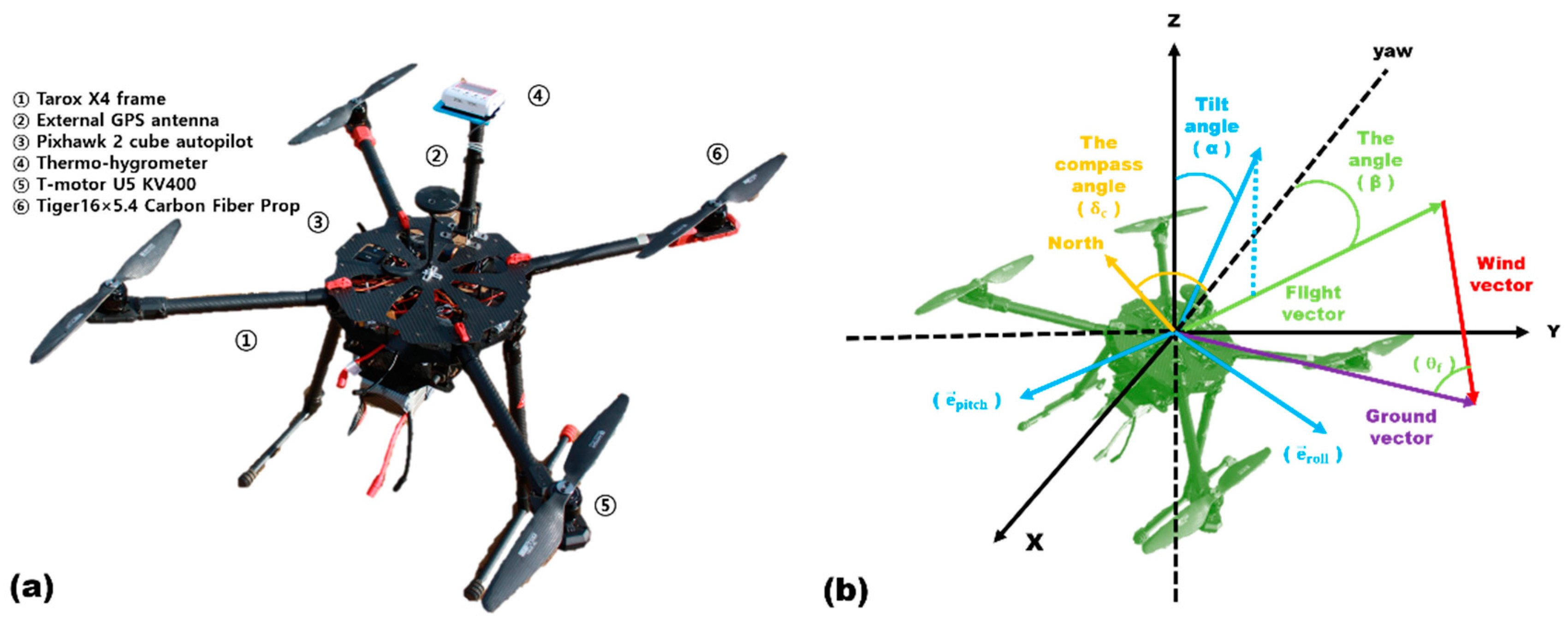
The UAV used in this study (Figure 1a) has four rotors and is capable of stable flight for up to 30 min with a fully charged battery. The UAV frame (Tarot X4, Wenzhou Aviation Technology Co., Wenzhou, China) is 960 mm × 960 mm × 320 mm with a weight of 1.6 kg. It was equipped with a Pixhawk 2 (3DR, USA) autopilot consisting of an external GPS (HERE + RTK GNSS, 3DR, Berkeley, CA, USA), a three-axis accelerometer, a three-axis gyroscope, a three-axis magnetometer, a temperature sensor, and a barometer to ensure stable position control. The IMU, which consisted of a three-axis accelerometer, and gyroscope automatically measured the UAV’s position data during the flight. Kalman filter calibrations were carried out in flight to decrease errors. The IMU and flight measurement unit (FMU) systems were separated to reduce sensor interference and to filter out high-frequency vibrations, reducing errors in the IMU data. The attitude data were recorded at 100 Hz for flight safety and GPS data (ground speed () and ground direction ()) were collected at 50 Hz. Flight stability was achieved using open source Mission Planner software with a horizontal hovering accuracy of ±0.01 m. UAV maximum elevation, horizontal movement, wind speed, and horizonal and vertical flight speeds were 2,000 m, 1,000 m, 10 m s−1, 6 m s−1, and 5 m s−1, respectively. To measure the air temperature, a thermo-hygrometer (HOBO H8 Pro, ONSET, Wareham, MA, USA) was installed on the rotary-wing of the UAV at 40 cm above the rotors. The rotary-wing UAV moves through the air by setting a tilt angle that is roughly proportional to speed. This tilt angle varies in real time to maintain stable flight. Therefore, the UAV-based wind vector can be indirectly estimated using the pitch, roll, and yaw angles measured by onboard sensors (IMU) for UAV’s attitude control without additional sensors for wind vector measurements [13,14,15,16,17,18,19,20,21].
The UAV-based wind vector was able to be calculated using the wind triangle (Figure 1b), which is widely used in navigation and estimates the wind vector using a flight and ground vector. The ground vector is measured directly from the UAV GPS receiver while the flight vector can be measured using an optical flow sensor or pitot tube [13,17,19]; however, these methods are not suitable for rotary-wing UAVs due to their flight speed () (which is lower than fixed-wing UAV), inconsistent flight direction (), and a wide range of tilt angle changes except for an examination [39].
Neuman and Bartholomai [21] have found a relationship between the tilt angle and flight speed () in wind tunnel experiments while Brosy et al. [20] have estimated flight speed assuming ground speed should be equal to flight speed under calm wind conditions where the wind speed is negligible (less than 1 m s−1) and have developed a relationship between the tilt angle and flight speed. We developed a relationship between the tilt angle and flight speed using the method given in Brosy et al. [20]. This is explained in detail in Section 3.2.
The tilt angle () can be estimated from the inverse scalar product of the normal unit vector to the XY-plane which is parallel to the ground and the cross product of the unit vectors as shown in Equation (10).
The angle between the projection of the vector onto the XY-plane, and the viewing direction of the UAV, defined as the negative normal vector is calculated using Equation (11).
To calculate the flight direction () whether the orthogonal vector is located in the left or right direction of the UAV’s viewing direction , Equation (12) is used. The flight direction can be estimated using and the compass angle () of the UAV viewing direction using Equation (13).
Finally, the UAV-based wind speed () is calculated using the wind triangle (Equation (14)) with the estimated flight vector (, ) and measured ground vector (, ).
The drift angle, , is equal to the difference between the ground direction (), which is measured by the GPS receiver and flight direction (). For detailed explanations of the wind direction () calculation, refer to Neuman and Bartholomai [21].
3. Results and Discussion
3.1. Sensible Heat Flux
Weather conditions at the study sites were dominated by anticyclones during the observation period (Table 1). In vegetated areas (GH1, GH2, GR1, and GR2), the mean wind speed was 2.0 to 2.8 m s−1 during the day, which weakened overnight. On rivers (KHR and SYR), weak winds (<2 m s−1) were observed during the day and night. For all sites, the heat flux and heat transfer coefficients were calculated indirectly using the bulk transfer method and validated using anemometer and SLS20 scintillometer measurements. As vertical fluctuations of horizontal wind and the thermal instability due to buoyancy vary with time, heat transfer coefficients clearly vary in response to temporal changes in atmospheric stability (Figure 2a). In vegetated areas, the heat transfer coefficient varied depending on atmospheric stability and roughness length z0m (m) from 6.0 × 10⁻³–3.0 × 10⁻² during the day to 2.0 × 10⁻³–10.0 × 10⁻³ overnight, which is consistent with values summarized according to surface conditions by Stull [40]. The heat transfer coefficient was larger in summer compared to winter. This is because the temperature difference between two heights is higher in summer than in winter. When the atmospheric stability was unstable ((zr−d0)/L < 0), the differences between heat transfer coefficients was larger than when the atmospheric stability was stable. However, the atmospheric stability was always unstable at river sites, because the water temperature was higher than the air temperature, even overnight. Consequently, heat transfer coefficients did not show significant differences between day and night.
Sensible heat flux was estimated using a heat transfer coefficient depending on the atmospheric stability ((zr−d0)/L), zero-plane displacement d0, and roughness length z0m, and compared with measurements from the 3D ultrasonic anemometer and SLS20. Figure 2b shows good agreement between directly and indirectly derived values, with a correlation coefficient of 0.94, mean bias of −1.26 W m−2, and RMSE of 19.9 W m−2, which is less than approximately 10% of the maximum measured value. We confirm that the bulk transfer method is useful to estimate UAV-based sensible heat flux.
3.2. Temperature and Wind Speed from Rotary-Wing UAV
The measurements from the UAV-mounted sensors (i.e., the anemometer and thermo-hygrometer) required validation because they were acquired from a moving body and were therefore liable to be affected by rotor wash. Palomaki et al. [15] have examined the effect of rotors on the wind vector from an anemometer located 30 cm above the rotary-wing UAV and found that the average bias due to the rotors was 0.5 m s−1 in indoor tests; however, rotor disturbance was found to be negligible at a height of 40–47 cm from the top of the rotary-wing UAV [14,41].
For the first part of the validation process, the profiles of temperature and humidity measured at 40 cm above the rotary-wing UAV were compared with those from the 10 m high meteorological tower that was equipped with an aerovane, a thermo-hygrometer, and surface temperature sensor (KWT1002, Wellbian system, Seoul, Korea) at sites CHR, WON, and SOK.
Figure 3 compares the air temperature and relative humidity between UAV-observed and AWS-observed data at a height of 10 m while hovering at a distance of 15 m from the AWS. UAV-observed temperatures are seen to be in good agreement with the AWS-observed temperatures, with a correlation coefficient of 0.98, mean bias of −1.1 °C, and RMSE of 1.79 °C. UAV-observed relative humidity measurements had lower agreement, with a correlation coefficient of 0.9, mean bias of 6.66%, and RMSE of 9.86%. AWS-observed relative humidity tended to be higher than the UAV-observed relative humidity during the day and lower during the night. The difference in agreement could be attributed to the accuracy of the temperature sensor (±0.2 °C) being higher than the accuracy of the relative humidity sensor (±2.5%). The UAV-observed atmospheric data was measured based on the volume of the air around the UAV rather than observations at a single point. Increasing the response time of the sensor could overcome this discrepancy [20].
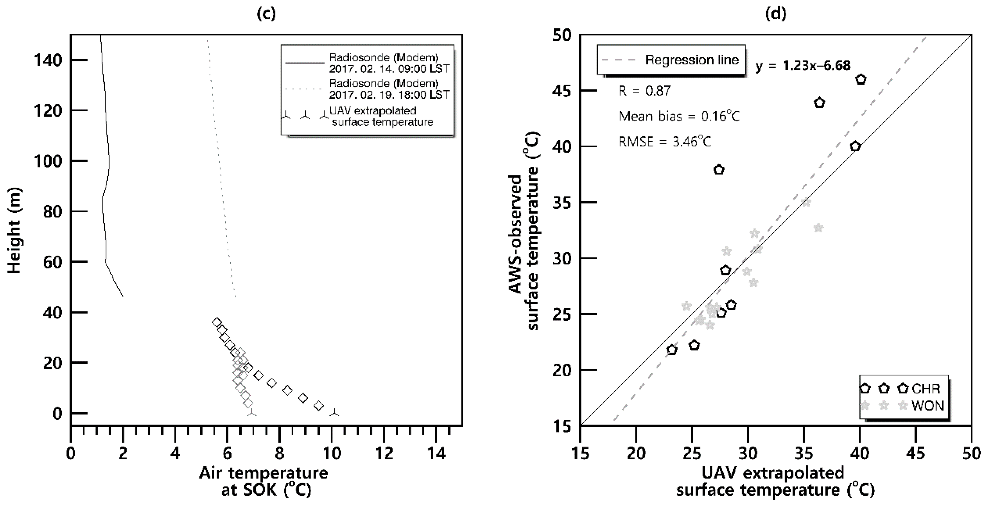
Radiosondes (DFM-09, Graw, Nürnberg, Germany; M10, Meteomodem, Ury, France) and a rotary-wing UAV were deployed simultaneously. Radiosondes provide fine resolution (one second) profiles of barometric pressure, temperature, wind, and relative humidity. Figure 4a–c shows vertical profiles of radiosonde-observed air temperature and vertical profiles of UAV-observed air temperature at CHR, WON, and SOK, respectively. Although radiosonde data loss and error were confirmed near the ground, there were small difference patterns between the profiles at nighttime. However, there were large difference patterns between the profiles during the daytime. These large difference patterns could be due to the time difference between the profiles. The radiosonde-observed air temperature had a temporal resolution of 1 s with an ascent rate of more than 6 m s−1, but UAV-observed temperatures were recorded while hovering at the same height for 1 min. When the surface is heated by solar radiation, the linearity of the air temperature gradient is not maintained. Martin et al. [11] have reported that it is possible to measure temperature, humidity, wind direction, wind speed, and even turbulence flux at a 10 cm vertical resolution using fixed-wing UAVs equipped with a very fast response speed sensor (30 Hz). These measurements were compared with measurements from the weather tower, wind profiler, and radiometer for verification. Because these observations were difficult to summarize from existing standard observation sensors, they reported only the usefulness and utility of the rotary-wing UAV. We examined the estimated surface skin temperature using linear extrapolation of the profile of UAV-observed air temperature and compared it with the observed surface temperature sensor (KWT1002, Wellbian system, Seoul, Korea) at CHR and WON. The correlation coefficient, mean bias, and RMSE were approximately 0.9, 0.2 °C, and 3.3 °C, respectively (Figure 4d); the latter shows that the largest difference between the temperatures was 10.5 °C at 10:00 local solar time (LST) on July 10, 2016. This is likely because of the specific heat difference between air and land surface and the land characteristics. After sunrise, land surface temperature usually begins to increase faster than air temperature due to the impact of solar radiation. The difference between surface temperatures at CHR is greater than those at WON because the land surface at the latter comprises stone and sand but that at the former comprises asphalt. Katz and Zhu [28] state that the surface skin temperature should be that defined at the height of thermal roughness length and that it may change from time to time even at a fixed location. A slight change in the height of the sensors can result in a large bias in the skin temperature because there is a sharp temperature gradient close to the surface. Thus, a proper extrapolation method to estimate surface temperature needs to be developed and could be the focus of further studies. In this study, an observed surface temperature was used for estimating UAV-based sensible heat flux from the bulk transfer method.
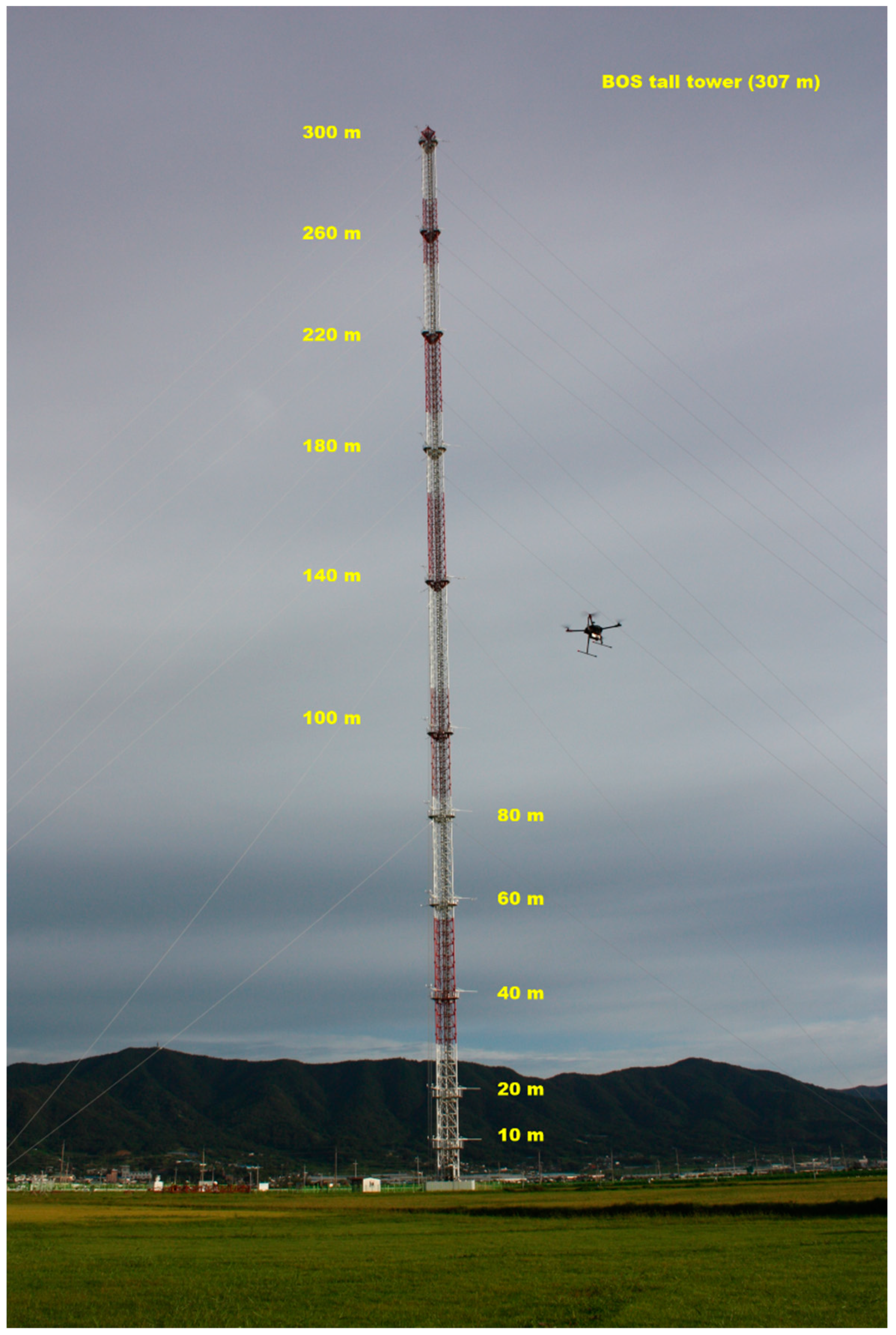
UAV-based wind speed was estimated by applying the flight vector () and the ground vector () to the wind triangle (Equation (14)) for the rotary-wing UAV at BOS and YHI. Notably, BOS has the second highest meteorological tower (307 m) in Asia (Figure 5). The accuracy of UAV-based wind speed depends on the accuracies of the flight and ground vectors. The ground vector is measured directly by the UAV’s GPS receiver. Therefore, a precise GPS receiver is very important for estimating UAV-based wind speed and flight performance. In this study, GPS equipped with real time kinematic (RTK) technology was installed to reduce error between the travel route and actual travel route measured by the GPS receiver to 3 cm from approximately 30 cm. For time synchronization between the GPS data (ground speed and ground direction) measured at 50 Hz and attitude data measured at 100 Hz, attitude data closest to the time of the GPS data were selected. The tilt angle was calculated using synchronized pitch and roll angles (50 Hz).
The ground speeds (50 Hz) recorded in the RTK GPS receiver were replaced with the flight speeds (. The tilt angle and flight speed were each averaged for one minute and then classified into 0.5 m s−1 intervals in this study. The tilt angle was also classified according to flight speed class and the number of flight speed classes was different for each case. Flight speeds from the highest class to the third highest class were averaged to determine the representative value of a case. Tilt angles were averaged in a similar manner.
Figure 6 shows scatter plots of the calculated tilt angles using Equation (10) and flight speeds that were replaced by ground speeds recorded in the RTK GPS receiver for 73 cases of calm winds (<3 knots) at BOS and YHI. The relationship between the tilt angle and the flight speed was estimated using the least squares method (Equation (15)) and is depicted by the solid black line in Figure 6. The difference in the relationships is possible due to hover characteristics. These are dependent on the diameter and weight of the UAV frame, tuning parameters that differ between UAV designs, and the quality of the GPS signal. Our relationship considers low flight speeds (<2 m s−1) and tilt angles (<4°).
For another 54 cases with wind (≥3 knots) at BOS and YHI, the tilt angles were calculated using pitch and roll angles measured during hovering at a distance of 15 m (for YHI this was 10 m) from the meteorological tower using Equation (10), and the flight speeds were calculated using the relationship we present in Equation (15). The calculated flight speeds and ground speeds were applied to Equation (14) to estimate the UAV-based wind speeds, which were then compared to those from the AWS at heights of 10, 20, and 40 m at BOS and 10 m at YHI.
Figure 7 shows the UAV-based wind speeds at BOS and YHI and the five-minute moving average AWS-observed wind speed. The correlation, mean bias, and RMSE between the UAV-based and AWS-observed wind speeds were 0.66, −0.15 m s−1, and 0.4 m s−1, respectively, at BOS, and 0.88, 0.34 m s−1, and 0.72 m s−1, respectively, at YHI. The relationship between the tilt angle and the flight speed was found to yield a reasonable flight speed for estimating UAV-based wind speed when compared to the AWS-observed wind speed. Examining the largest mean bias, the RMSEs between the UAV-based and AWS-observed wind speeds for each time period were −0.04 m s−1 and 0.7 m s−1, respectively, occurring at approximately 11:00–13:00 LST. The mean bias and RMSE (–0.7 m s−1 and 0.9 m s−1, respectively) between the UAV-based and AWS-observed wind speeds at 40 m were larger compared to at 10 m (0.1 m s−1 and 0.4 m s−1, respectively). These errors could have been caused by many factors, including atmospheric conditions such as wind gusts (i.e., the wind speed cannot be negligible as assumed), sharp wind variation over the distance between the rotary-wing UAV and anemometer, and time discrepancies between the GPS and IMU due to delays in GPS data. Shimura et al. [14] noted an error when turbulence was strong due to increased wind shear. Neumann and Bartholomai [21] reported an RMSE of ±0.6 m s−1 when hovering 5 m away from an ultrasonic anemometer and an RMSE of ±0.3 m s−1 at 2 m. Palomaki et al. [15] reported an RMSE of 0.5 m s−1 when the wind speed was 0–5 m s−1 while Brosy et al. [20] found an RMSE of 0.7 m s−1 and a maximum standard deviation of 2 m s−1. Palomaki et al. [15] have stated that stable hovering is important for accurate wind speed estimation. For this, it is necessary to optimize weight, diameter, quality of GPS signal, and various tuning parameters of the UAV.
3.3. Heat Flux Based on Rotary-Wing UAV Hovering
Estimation of the sensible heat flux based on rotary-wing UAV hovering was tested at two wind speeds. The AWS-observed wind speed was tested at SOK during international collaborative experiments for the Pyeongchang 2018 Olympic Winter Games (https://weather.msfc.nasa.gov/sport/icepop2018/) in February and March 2018 while UAV-based wind speeds were tested at BOS in September 2018 and at YHI in November and December 2018. The BOS site is the largest observatory in Korea with a 307 m meteorological tower (Figure 5) equipped with a thermo-hygrometer (5628, Fluke; HMP155, Vaisala) and two-dimensional ultrasonic anemometer (UA-2D, Thies Clima, Göttingend, Germany; 05103, R. M. Young, U.S.A.) with 11 heights that have projecting rods oriented in three directions. A three-dimensional ultrasonic anemometer, infrared gas analyzer, and net radiometer are also installed at the surface (2.5 m), as well as at 60, 140, and 300 m. The heat transfer coefficient and sensible heat flux were estimated using the bulk transfer method with AWS-observed surface temperature, UAV-observed air temperature, AWS-observed wind speed, or UAV-based wind speed.
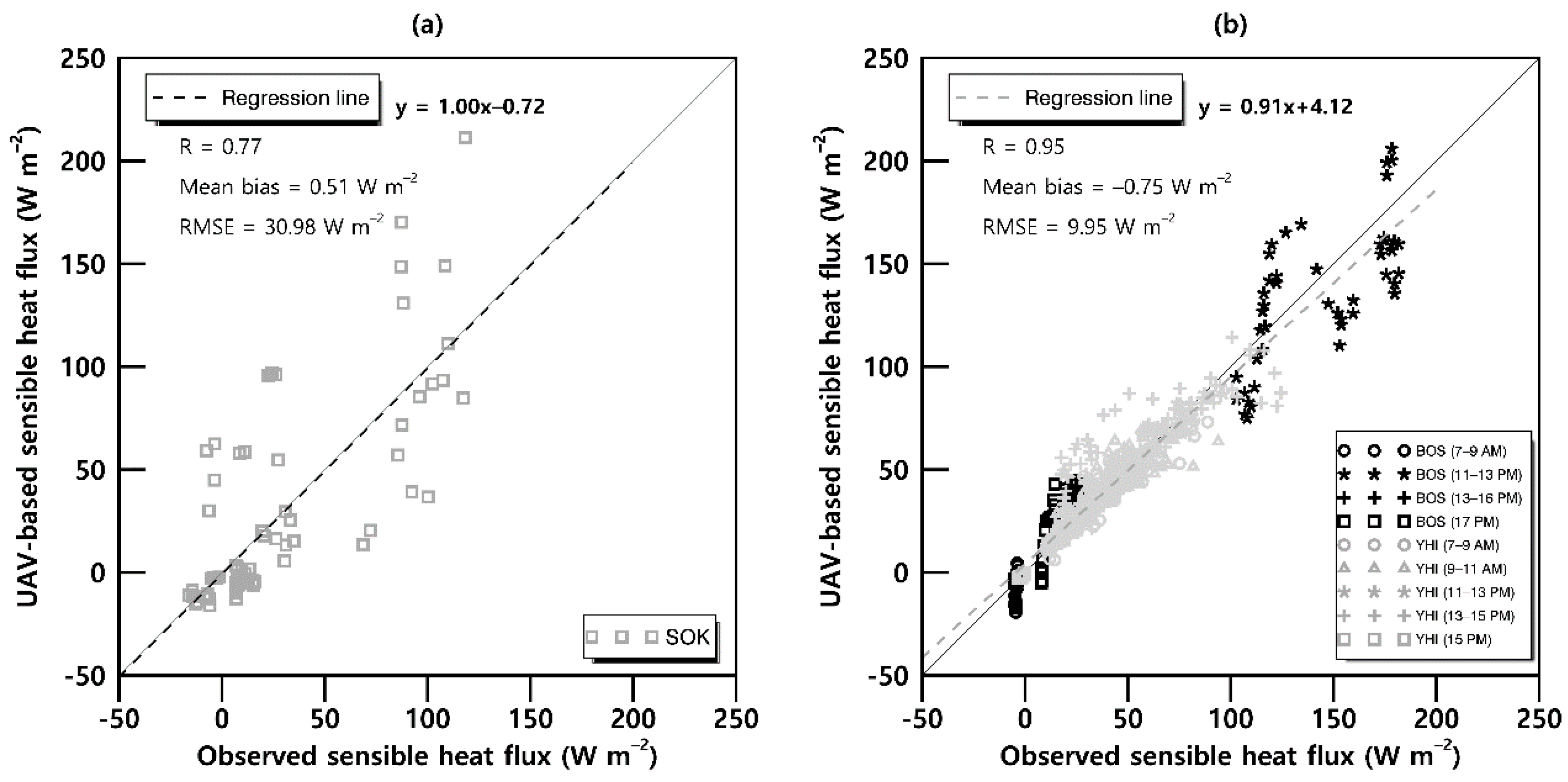
UAV-based heat fluxes (Hb_AWSUAV) were calculated by applying the heat transfer coefficient, AWS-observed wind speed, AWS-observed surface temperature, and UAV-observed air temperature to Equation (1b) and comparing the result with the sensible heat flux H measured directly with eddy covariance equipment and calculated according to Equation (1a) (Figure 8a). The raw data measured at 10 Hz by the anemometer were subjected to peak inspection and direction correction according to the quality control method of Vickers and Mahrt [42]. The eddy covariance method was applied to calculate heat flux following double coordinate conversion. The correlation coefficient between H and Hb_AWSUAV (0.77), mean bias (0.51 W m−2), and RMSE (30.98 W m−2) were within 20% of the maximum H.
UAV-based heat fluxes (Hb_UAVUAV) were calculated by applying the heat transfer coefficient, UAV-based wind speed, AWS-observed surface temperature, and UAV-observed air temperature to Equation (1b) and comparing the results with H. Figure 8b presents the five-minute moving averaged Hb_UAVUAV and Husing different symbols for time. The correlation coefficient (0.95), mean bias (−0.75 W m−2), and RMSE (10 W m−2) between H and Hb_UAVUAV were within 5% of the maximum H. The largest mean bias and RMSE between the Hb_UAVUAV and H were −3.6 W m−2 and 18.5 W m−2, respectively, occurring between 11:00–13:00 LST. This error can be explained by Equation (1b). We confirmed that the mean bias and RMSE between UAV-based and AWS-observed wind speeds were relatively the largest at that time, and those were −0.04 ms−1 and 0.7 ms−1. The mean AWS-observed wind speed was 3 ms−1 between 11:00–13:00 LST, which was the strongest compared to the other times. The mean bias and RMSE were −0.9 °C and 1.2 °C between UAV-observed and AWS-observed temperatures, respectively, and were the largest compared to the other times. Knuth and Cassano [24] calculated the sensible heat flux by applying UAV-observed pressure, temperature, and wind speed to the integral method and examined the sensitivity of each UAV-observed measurement on the calculated heat flux using random perturbations for 500 repetitions. They found that the standard deviation for most flight days was within 5–15 W m−2. Lee et al. [43] estimated the horizontal variability in heat flux surrounding meteorological towers by applying the rotary-wing UAV-observed pressure, temperature, and relative humidity to the conditional sampling technique. Comparisons between UAV-based with independent eddy covariance sensible heat flux agreed to within 5–10 W m−2. When comparing UAV-based and large eddy simulation-modeled heat flux, differences over a few isolated locations were as large as 50–70 W m−2. Lee et al. [43] have also reported that these discrepancies are likely caused by the advection of high thin cirrus clouds, because large eddy simulations were unable to advect the cloud cover across the sensible heat flux that was seen in the observations.
3.4. Atmospheric Boundary Layer Height Based on Rotary-Wing UAV Hovering
Reineman et al. [23] have demonstrated measuring UAV-based turbulent flux and the development of the ABL. Furthermore, Zhang et al. [44] have reported that low soil moisture, high surface sensible heat flux, high Bowen ratio, and low latent heat flux generally facilitate ABL height growth in the afternoon. Low soil moisture tends to favor ABL growth by partitioning more solar radiation to sensible heat flux [45]. Seidel et al. [46] calculated ABL height using seven common methods and found large uncertainties with respect to these methods. Turbulence is generally responsible for the mixing processes in the ABL, and the turbulent motions affect the vertical redistribution of momentum and heat. Regardless of the synoptic condition, the ABL height is mostly determined by the activation of atmospheric turbulence by the supply of thermal energy from the surface to the atmosphere in areas where the heat flux is strong. Therefore, accurate sensible heat flux measurements are important for understanding ABL structural processes. The most widely used and simplest indirect method of estimating heat flux is via the bulk aerodynamic approach, which is based on the bulk transfer formula (Equation (1b)). In radiosonde data, the height of the maximum gradient of vertical change in potential temperature is defined as the ABL height. The relationship between UAV-based heat flux and radiosonde-based ABL height was found for nine cases at SOK, BOS, and YHI.
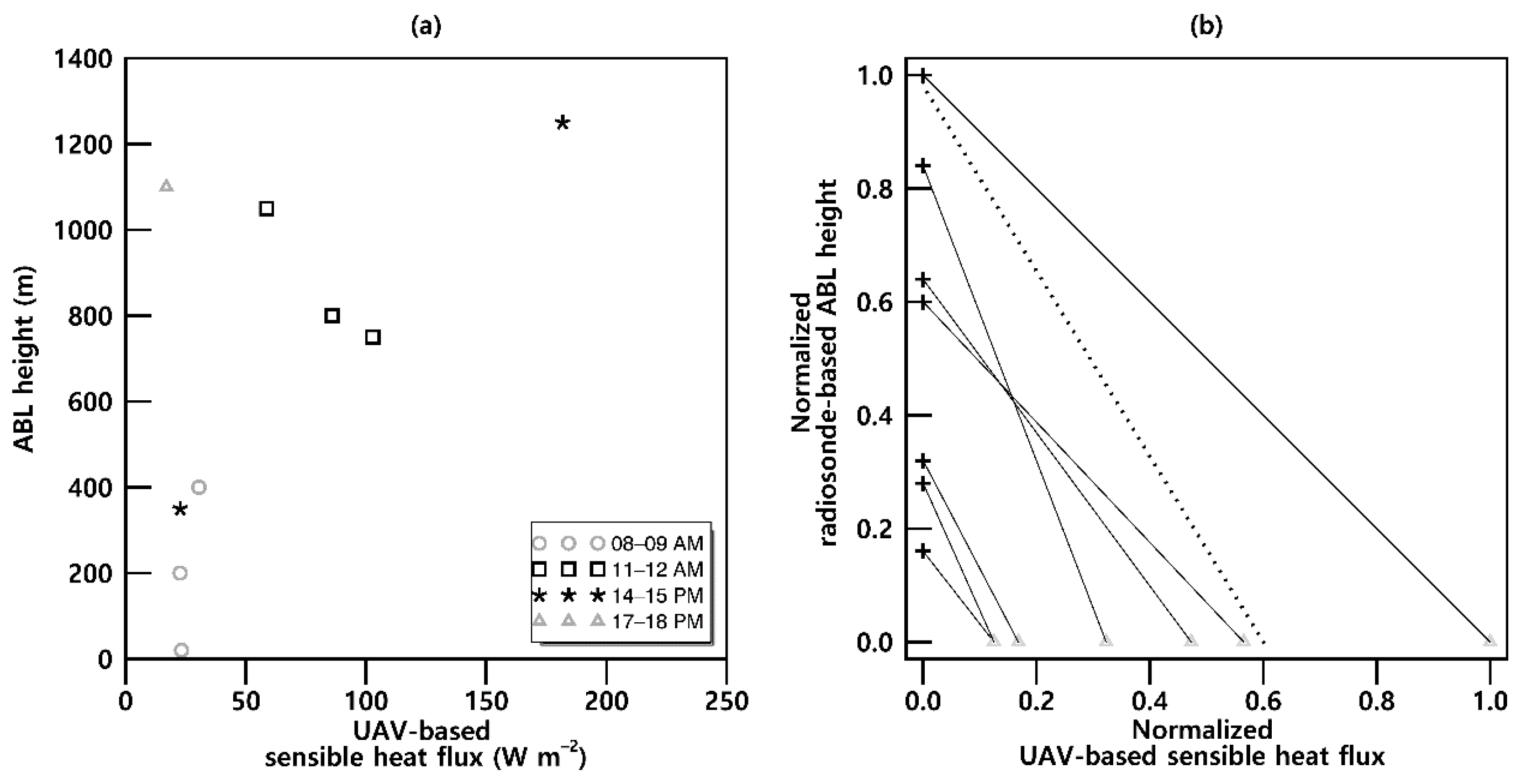
Figure 9a shows radiosonde-based ABL heights and UAV-based sensible heat flux over time. The ABL height increased with sensible heat flux due to surface heating following sunrise. The UAV-based sensible heat fluxes were between 20–30 W m−2 and radiosonde-observed ABL heights were between 20–250 m between 8:00 and 9:00 LST. However, UAV-based heat flux was 30.5 W m−2 and radiosonde-observed ABL height was 400 m at 9:00 LST on November 30, 2018. It has been shown that ABL heights can grow quickly in the morning and reach around 1200 m because of the cloud-free convective conditions, with surface skin temperatures reaching 30 °C. UAV-based heat flux increased to more than 100 Wm−2 between 11:00 and 12:00 LST. As a result, the ABL height of 20–400 m rapidly increased to 750–1,050 m. When the UAV-based heat flux was 190 W m−2 at 14:00 LST on September 11, 2018 in BOS, the ABL grew further to 1250 m. These results are consistent with a previous study where a heat flux of 321 W m−2 increased the ABL height from 457 m to 625 m, i.e., an increase of 39% [25]. The increase in ABL height was due to the increase in heat flux, which was caused by an increase in the temperature difference between the two profiles [24]. By contrast, the radiosonde-based ABL height was 350 m at 15:00 LST on December 15, 2018 at YHI. This occurred because the surface sensible heat flux was low due to clouds and clouds are generally associated with lower ABL heights.
When the surface skin cools due to nocturnal radiation processes, the sensible heat flux becomes negative instead of positive. However, while the UAV-based heat flux was 17 W m−2, the ABL grew to 1100 m at 18:00 LST on September 11, 2018 in BOS, caused by strong winds blowing from the south coast. Strong wind shear within the ABL facilitated dynamic growth, turbulent kinetic energy was generated in the surface layer, and heat flux increased with height. Many previous studies have stated that cloudiness, heating of the ground surface, and variability in surface characteristics can affect the evolution of the ABL. Furthermore, daytime ABL height is positively correlated with surface skin temperature [47]. Conversely, turbulent flux was measured from aircraft following approximately linear gradient profiles [48,49,50].
The linear relationships between normalized heat flux (dimensionless) and normalized ABL height are shown in Figure 9b. Heat flux is assumed to decrease with height and reach zero at the top of the ABL. As shown by the gray lines, the slopes of the straight lines formed by normalized heat flux and ABL heights are the rate of change in the heat flux according to height [40]. By averaging all these slopes, the representative heat flux rate of change was approximately 1.6, as shown by the dashed black line. Therefore, it is possible to estimate ABL height using the UAV-based sensible heat flux.
Our results confirm that the ABL height varies linearly with the surface heat flux and indirect estimation of the ABL height using a UAV-based heat flux is possible; however, it is necessary to analyze the relationship between sensible heat flux and ABL height using more UAV observation cases in future research.
4. Conclusions
Accurate measurement of vertical profiles of temperature, moisture, and wind in the lower ABL at high spatial and temporal resolutions are important for understanding ABL development mechanisms. In this study, we show that these profiles, and estimates of wind speed, heat flux, and ABL height can be achieved using a rotary-wing UAV equipped with a temperature/humidity sensor approximately 40 cm above the UAV. We confirmed that UAV-observed temperatures and relative humidity were in good agreement with the AWS-observed temperatures and relative humidity, with correlation coefficients of 0.98 and 0.9, and a mean bias of −1.05 °C and 6.66%, respectively. Our own relationship (Equation (15)) between flight speed and tilt angle was estimated under calm wind conditions and compared with previous studies. Flight speed was calculated for wind conditions using our relationship and the UAV-based wind speed was estimated using the flight and ground speeds with the wind triangle. The UAV-based wind speeds agreed with the AWS-based wind speeds within an error of 10%. Accurate wind measurements provided excellent UAV-based heat flux with a mean bias of −0.75 W m−2 and RMSE less than 10 W m−2. Radiosonde-based ABL height increased with the UAV-based heat flux by heating the surface after sunrise and vice versa. The relationship between UAV-based heat flux and radiosonde-based ABL height can be used to estimate ABL height. We confirmed the usefulness of estimating UAV-based wind speed, heat flux, and ABL height; however, additional studies are needed to further evaluate our newly proposed approach. The well-known Monin–Obukhov similarity theory is mostly used to close bulk transfer parameterization. However, it is not easy to obtain an accurate surface skin temperature to determine surface flux parameterization based on the Monin–Obukhov similarity and bulk transfer method. The estimation of surface skin temperature was examined using linear extrapolation of the profile of the UAV-observed temperature and evaluated with the observed surface temperature sensor. The correlation coefficient and RMSE showed agreement (0.9 and 3.5 °C, respectively), but the largest difference between the temperatures was 10.5 °C at 10:00 LST on July 10, 2016. This could be due to specific heat difference between the air and land surface and land characteristics. This is a limitation of our newly proposed approach based on the bulk transfer method, which requires surface temperature. Thus, future studies are needed to estimate surface temperatures using a UAV. Utilizing a thermal camera (Duo pro R 640, FLIR, Wilsonville, OR, USA) to observe surface temperature directly might be a viable solution. Other solutions include using the gradient method [33] or the profile method [51], which do not require surface temperature and roughness length. Utilizing UAVs to estimate wind speed, heat flux, and ABL height has advantages over existing standard observation methods. They have the advantage of low-altitude flights at no risk to human pilots and can capture the evolution of ABL over transition zones such as air-sea boundaries. UAV can also help determine the horizontal variability of heat flux at a regional scale. Consequently, UAV can play an important role in acquiring ABL height and near surface atmospheric flux, especially in extreme conditions where satellite-derived flux products are unreliable. UAV-based wind vectors supplement the data of the area that cannot be observed by the UHF wind profiler.
Author Contributions
M.-S.K. designed the research, processed the meteorological data, and wrote the manuscript. M.-S.K. and B.H.K. contributed scientific discussion. B.H.K. supervised this research. M.-S.K. and B.H.K. contributed to reviewing the manuscript.
Funding
This work was funded by the Korea Meteorological Administration Research and Development Program under grant KMI2018-06310.
Acknowledgments
We would like to thank the editor and three anonymous reviewers for their comments, which have greatly improved this manuscript. We thank the Korea Meteorological Administration for the dataset.
Conflicts of Interest
The authors declare no conflict of interest.
References
- Arya, S.P. Introduction to Micrometeorology; Academic Press: San Diego, CA, USA, 1988; ISBN 9788578110796. [Google Scholar]
- Yi, C.; Davis, K.J.; Berger, B.W.; Bakwin, P.S.; Yi, C.; Davis, K.J.; Berger, B.W.; Bakwin, P.S. Long-term observations of the dynamics of the continental planetary boundary layer. J. Atmos. Sci. 2001, 58, 1288–1299. [Google Scholar] [CrossRef]
- Yi, C.; Davis, K.J.; Bakwin, P.S.; Denning, A.S.; Zhang, N.; Desai, A.; Lin, J.C.; Gerbig, C.; Yi, C. Observed covariance between ecosystem carbon exchange and atmospheric boundary layer dynamics at a site in northern Wisconsin. J. Geophys. Res. 2004, 109, D08302. [Google Scholar] [CrossRef]
- Kalverla, P.C.; Duine, G.J.; Steeneveld, G.J.; Hedde, T.; Kalverla, P.C.; Duine, G.J.; Steeneveld, G.J.; Hedde, T. Evaluation of the weather research and forecasting model in the Durance Valley complex terrain during the KASCADE field campaign. J. Appl. Meteorol. Climatol. 2016, 55, 861–882. [Google Scholar] [CrossRef]
- Lehner, M.; Whiteman, C.D.; Hoch, S.W.; Jensen, D.; Pardyjak, E.R.; Leo, L.S.; Di Sabatino, S.; Fernando, H.J.S.; Lehner, M.; Whiteman, C.D.; et al. A case study of the nocturnal boundary layer evolution on a slope at the foot of a desert mountain. J. Appl. Meteorol. Climatol. 2015, 54, 732–751. [Google Scholar] [CrossRef]
- Rennó, N.O.; Williams, E.R. Quasi-lagrangian measurements in convective boundary layer plumes and their implications for the calculation of CAPE. Mon. Weather Rev. 1995, 123, 2733–2742. [Google Scholar] [CrossRef]
- Spiess, T.; Bange, J.; Buschmann, M.; Vörsmann, P. First application of the meteorological Mini-UAV “M2AV”. Meteorol. Zeitschrift 2007, 16, 159–169. [Google Scholar] [CrossRef] [PubMed]
- Holland, G.J.; McGeer, T.; Youngren, H.; Holland, G.J.; McGeer, T.; Youngren, H. Autonomous aerosondes for economical atmospheric soundings anywhere on the globe. Bull. Am. Meteorol. Soc. 1992, 73, 1987–1998. [Google Scholar] [CrossRef]
- Valero, F.P.J.; Bucholtz, A.; Bush, B.C.; Pope, S.K.; Collins, W.D.; Flatau, P.; Strawa, A.; Gore, W.J.Y. Atmospheric radiation measurements enhanced shortwave experiment (ARESE): Experimental and data details. J. Geophys. Res. Atmos. 1997, 102, 29929–29937. [Google Scholar] [CrossRef]
- Lawrence, D.A.; Balsley, B.B.; Lawrence, D.A.; Balsley, B.B. High-resolution atmospheric sensing of multiple atmospheric variables using the DataHawk small airborne measurement system. J. Atmos. Ocean. Technol. 2013, 30, 2352–2366. [Google Scholar] [CrossRef]
- Martin, S.; Bange, J.; Beyrich, F. Meteorological profiling of the lower troposphere using the research UAV “M2AV Carolo”. Atmos. Meas. Tech. 2011, 4, 705–716. [Google Scholar] [CrossRef]
- Mayer, S.; Sandvik, A.; Jonassen, M.O.; Reuder, J. Atmospheric profiling with the UAS SUMO: A new perspective for the evaluation of fine-scale atmospheric models. Meteorol. Atmos. Phys. 2012, 116, 15–26. [Google Scholar] [CrossRef]
- van den Kroonenberg, A.; Martin, T.; Buschmann, M.; Bange, J.; Vörsmann, P. Measuring the wind vector using the autonomous mini aerial vehicle M2AV. J. Atmos. Ocean. Technol. 2008, 25, 1969–1982. [Google Scholar] [CrossRef]
- Shimura, T.; Inoue, M.; Tsujimoto, H.; Sasaki, K.; Iguchi, M.; Shimura, T.; Inoue, M.; Tsujimoto, H.; Sasaki, K.; Iguchi, M. Estimation of wind vector profile using a hexarotor unmanned aerial vehicle and its application to meteorological observation up to 1000 m above Surface. J. Atmos. Ocean. Technol. 2018, 35, 1621–1631. [Google Scholar] [CrossRef]
- Palomaki, R.T.; Rose, N.T.; van den Bossche, M.; Sherman, T.J.; De Wekker, S.F.J. Wind estimation in the lower atmosphere using multirotor aircraft. J. Atmos. Ocean. Technol. 2017, 34, 1183–1191. [Google Scholar] [CrossRef]
- Divitiis, N. Wind estimation on a lightweight vertical-takeoff-and-landing uninhabited vehicle. J. Aircr. 2003, 40, 759–767. [Google Scholar] [CrossRef]
- Molnar, A.; Stojcsics, D. New approach of the navigation control of small size UAVs. In Proceedings of the 19th International Workshop on Robotics in Alpe-Adria-Danube Region (RAAD 2010), Balatonfured, Hungary, 24–26 June 2010; IEEE: Budapest, Hungary, 2010; pp. 125–129. [Google Scholar]
- Pachter, M.; Ceccarelli, N.; Chandler, P. Estimating MAV’s heading and the wind speed and direction using GPS, inertial, and air speed measurements. In AIAA Guidance, Navigation and Control Conference and Exhibit; American Institute of Aeronautics and Astronautics: Hawaii, HI, USA, 2008. [Google Scholar]
- Rodriguez, A.; Andersen, E.; Bradley, J.; Taylor, C. Wind estimation using an optical flow sensor on a miniature air vehicle. In AIAA Guidance, Navigation and Control Conference and Exhibit; American Institute of Aeronautics and Astronautics: South Carolina, CA, USA, 2007. [Google Scholar]
- Brosy, C.; Krampf, K.; Zeeman, M.; Wolf, B.; Junkermann, W.; Schäfer, K.; Emeis, S.; Kunstmann, H. Simultaneous multicopter-based air sampling and sensing of meteorological variables. Atmos. Meas. Tech. 2017, 10, 2773–2784. [Google Scholar] [CrossRef] [Green Version]
- Neumann, P.P.; Bartholmai, M. Real-time wind estimation on a micro unmanned aerial vehicle using its inertial measurement unit. Sensors Actuators A Phys. 2015, 235, 300–310. [Google Scholar] [CrossRef]
- Bonin, T.; Chilson, P.; Zielke, B.; Fedorovich, E. Observations of the Early Evening Boundary-Layer Transition Using a Small Unmanned Aerial System. Bound-Lay Meteorol. 2013, 146, 119–132. [Google Scholar] [CrossRef]
- Reineman, B.D.; Lenain, L.; Statom, N.M.; Melville, W.K.; Reineman, B.D.; Lenain, L.; Statom, N.M.; Melville, W.K. Development and testing of instrumentation for UAV-based flux measurements within terrestrial and marine atmospheric boundary layers. J. Atmos. Ocean. Technol. 2013, 30, 1295–1319. [Google Scholar] [CrossRef]
- Knuth, S.L.; Cassano, J.J. Estimating sensible and latent heat fluxes using the integral method from in situ aircraft measurements. J. Atmos. Ocean. Technol. 2014, 31, 1964–1981. [Google Scholar] [CrossRef]
- Båserud, L.; Reuder, J.; Jonassen, M.O.; Kral, S.T.; Paskyabi, M.B.; Lothon, M. Proof of concept for turbulence measurements with the RPAS SUMO during the BLLAST campaign. Atmos. Meas. Tech. 2016, 9, 4901–4913. [Google Scholar] [CrossRef] [Green Version]
- Garratt, J.R. Review: The atmospheric boundary layer. Earth-Science Rev. 1994, 37, 89–134. [Google Scholar] [CrossRef]
- Deardorff, J.W. Parameterization of the planetary boundary layer for use in general circulation models 1. Mon. Weather Rev. 1972, 100, 93–106. [Google Scholar] [CrossRef]
- Katz, J.; Zhu, P. Evaluation of surface layer flux parameterizations using in-situ observations. Atmos. Res. 2017, 194, 150–163. [Google Scholar] [CrossRef]
- Monin, A.S.; Obukhov, A.M. Basic laws of turbulent mixing in the surface layer of the atmosphere. Tr. Akad. Nauk SSSR Geophiz. Inst. 1954, 24, 163–187. [Google Scholar]
- Stanhill, G. A simple instrument for the field measurement of turbulent diffusion flux. J. Appl. Meteorol. 1969, 8, 509–513. [Google Scholar] [CrossRef]
- Brümmer, B.; Schröder, D.; Launiainen, J.; Vihma, T.; Smedman, A.S.; Magnusson, M. Temporal and spatial variability of surface fluxes over the ice edge zone in the northern Baltic Sea. J. Geophys. Res. 2002, 107, 3096. [Google Scholar] [CrossRef]
- Verkaik, J.W.; Holtslag, A.A.M. Wind profiles, momentum fluxes and roughness lengths at Cabauw revisited. Bound-Lay Meteorol. 2007, 122, 701–719. [Google Scholar] [CrossRef]
- Businger, J.A.; Wyngaard, J.C.; Izumi, Y.; Bradley, E.F.; Businger, J.A.; Wyngaard, J.C.; Izumi, Y.; Bradley, E.F. Flux-profile relationships in the atmospheric surface layer. J. Atmos. Sci. 1971, 28, 181–189. [Google Scholar] [CrossRef]
- Launiainen, J.; Vihma, T. Derivation of turbulent surface fluxes—An iterative flux-profile method allowing arbitrary observing heights. Environ. Softw. 1990, 5, 113–124. [Google Scholar] [CrossRef]
- De Bruin, H.A.R.; Van Den Hurk, B.J.J.M.; Kohsiek, W. The scintillation method tested over a dry vineyard area. Bound-Lay Meteorol. 1995, 76, 25–40. [Google Scholar] [CrossRef]
- Kanda, M.; Moriwaki, R.; Roth, M.; Oke, T. Area-averaged sensible heat flux and a new method to determine Zero-Plane displacement length over an urban surface using scintillometry. Bound-Laye Meteorol. 2002, 105, 177–193. [Google Scholar] [CrossRef]
- Nieveen, J.P.; Green, A.E. Measuring sensible heat flux density over pasture using the ct2-Profile method. Bound-Lay Meteorol. 1999, 91, 23–35. [Google Scholar] [CrossRef]
- Weiss, A.I.; Hennes, M.; Rotach, M.W. Derivation of refractive index and temperature gradients from optical scintillometry to correct atmospherically induced errors for highly precise geodetic measurements. Surv. Geophys. 2001, 22, 589–596. [Google Scholar] [CrossRef]
- Arain, B.; Kendoul, F. Real-time wind speed estimation and compensation for improved flight. IEEE Trans. Aerosp. Electron. Syst. 2014, 50, 1599–1606. [Google Scholar] [CrossRef]
- Stull, R.B. An Introduction to Boundary Layer Meteorology; Kluwer Academic Publishers: Dordrecht, The Netherlands, 1988; ISBN 978-94-009-3027-8. [Google Scholar]
- Alvarado, M.; Gonzalez, F.; Fletcher, A.; Doshi, A. Towards the development of a low cost airborne sensing system to monitor dust particles after blasting at open-pit mine sites. Sensors 2015, 15, 19667–19687. [Google Scholar] [CrossRef] [PubMed]
- Vickers, D.; Mahrt, L.; Vickers, D.; Mahrt, L. Quality control and flux sampling problems for tower and aircraft data. J. Atmos. Ocean. Technol. 1997, 14, 512–526. [Google Scholar] [CrossRef]
- Lee, T.R.; Buban, M.; Dumas, E.; Baker, C.B.; Lee, T.R.; Buban, M.; Dumas, E.; Baker, C.B. A new technique to estimate sensible heat fluxes around micrometeorological towers using small unmanned aircraft systems. J. Atmos. Ocean. Technol. 2017, 34, 2103–2112. [Google Scholar] [CrossRef]
- Zhang, W.; Guo, J.; Miao, Y.; Liu, H.; Song, Y.; Fang, Z.; He, J.; Lou, M.; Yan, Y.; Li, Y.; et al. On the summertime planetary boundary layer with different thermodynamic stability in China: A radiosonde perspective. J. Clim. 2018, 31, 1451–1465. [Google Scholar] [CrossRef]
- Wang, X.Y.; Wang, K.C. Estimation of atmospheric mixing layer height from radiosonde data. Atmos. Meas. Tech. 2014, 7, 1701–1709. [Google Scholar] [CrossRef] [Green Version]
- Seidel, D.J.; Ao, C.O.; Li, K. Estimating climatological planetary boundary layer heights from radiosonde observations: Comparison of methods and uncertainty analysis. J. Geophys. Res. 2010, 115, D16113. [Google Scholar] [CrossRef]
- Zhang, Y.; Seidel, D.J.; Zhang, S.; Zhang, Y.; Seidel, D.J.; Zhang, S. Trends in planetary boundary layer height over Europe. J. Clim. 2013, 26, 10071–10076. [Google Scholar] [CrossRef]
- Lenschow, D.H.; Li, X.S.; Zhu, C.J.; Stankov, B.B. The Stably Stratified Boundary Layer over the Great Plains. In Topics in Micrometeorology. A Festschrift for Arch Dyer; Springer: Dordrecht, The Netherlands, 1988; pp. 95–121. [Google Scholar]
- Mahrt, L. Vertical structure and turbulence in the very stable boundary layer. J. Atmos. Sci. 1985, 42, 2333–2349. [Google Scholar] [CrossRef]
- Tjernström, M. Turbulence length scales in stably stratified free shear flow analyzed from slant aircraft profiles. J. Appl. Meteorol. 1993, 32, 948–963. [Google Scholar] [CrossRef]
- Nieuwstadt, F. The computation of the friction velocity u * and the temperature scale T * from temperature and wind velocity profiles by least-square methods. Bound-Lay Meteorol. 1978, 14, 235–246. [Google Scholar] [CrossRef]
Figure 1.
(a) The quadcopter used in this study and all sensors installed on it (1–5) and (b) the relationship between the wind triangle and flight, ground, wind vectors, and tilt angle (α) of the UAV. The viewing direction of the UAV relative to the north is the compass angle (δc).
Figure 1.
(a) The quadcopter used in this study and all sensors installed on it (1–5) and (b) the relationship between the wind triangle and flight, ground, wind vectors, and tilt angle (α) of the UAV. The viewing direction of the UAV relative to the north is the compass angle (δc).

Figure 2.
(a) Heat transfer coefficients as functions of atmospheric stability ((zr−d0)/L) for different surfaces and (b) comparison of sensible heat fluxes estimated by the bulk transfer method with the sensible heat flux measured by 3D ultrasonic anemometer and SLS20 at sites KHR and SYR.
Figure 2.
(a) Heat transfer coefficients as functions of atmospheric stability ((zr−d0)/L) for different surfaces and (b) comparison of sensible heat fluxes estimated by the bulk transfer method with the sensible heat flux measured by 3D ultrasonic anemometer and SLS20 at sites KHR and SYR.

Figure 3.
Comparison of UAV-observed air temperature (a) and relative humidity (b) with corresponding automatic weather system (AWS)-observed air temperature and relative humidity at 10 m.
Figure 3.
Comparison of UAV-observed air temperature (a) and relative humidity (b) with corresponding automatic weather system (AWS)-observed air temperature and relative humidity at 10 m.

Figure 4.
Comparison of UAV-observed air temperature profiles (black and gray symbols) with radiosonde-observed air temperature profiles (black solid and gray dotted lines) at (a) CHR, (b) WON, and (c) SOK; (d) a comparison of extrapolated surface temperature using UAV-observed air temperature profiles with AWS-observed surface temperatures.


Figure 5.
Rotary-wing UAV using a local coordinate system at the BOS observatory. The roll, pitch, and yaw angles are the rotations about the X, Y, and Z axes, respectively.
Figure 5.
Rotary-wing UAV using a local coordinate system at the BOS observatory. The roll, pitch, and yaw angles are the rotations about the X, Y, and Z axes, respectively.

Figure 6.
Regression function of the relationship between flight speed and tilt angle as experimentally determined during calm wind conditions (<1 m s−1). The solid black line represents the fitted regression function and the gray error bars indicate standard deviations.
Figure 6.
Regression function of the relationship between flight speed and tilt angle as experimentally determined during calm wind conditions (<1 m s−1). The solid black line represents the fitted regression function and the gray error bars indicate standard deviations.

Figure 7.
Comparison of UAV-based wind speeds with AWS-observed wind speeds at BOS and YHI.

Figure 8.
(a) Comparison of UAV-based heat fluxes (Hb_AWSUAV) with observed heat fluxes (H) at SOK and (b) comparison of UAV-based heat fluxes (Hb_UAVUAV) with observed heat fluxes (H) at BOS and YHI.
Figure 8.
(a) Comparison of UAV-based heat fluxes (Hb_AWSUAV) with observed heat fluxes (H) at SOK and (b) comparison of UAV-based heat fluxes (Hb_UAVUAV) with observed heat fluxes (H) at BOS and YHI.

Figure 9.
(a) Radiosonde-observed atmospheric boundary layer (ABL) heights and UAV-based heat fluxes (Hb_UAVUAV) estimated using the bulk transfer method and (b) relationship between normalized ABL height and normalized sensible heat flux.
Figure 9.
(a) Radiosonde-observed atmospheric boundary layer (ABL) heights and UAV-based heat fluxes (Hb_UAVUAV) estimated using the bulk transfer method and (b) relationship between normalized ABL height and normalized sensible heat flux.


Table 1.
Observation periods and characteristics for each site.
| Site | Period | Surface | d0 (m) | z0m (m) | Synoptic Condition | Main Instruments |
|---|---|---|---|---|---|---|
| GH1 | 2006.08.08–2006.08.11 | Reed | 2.1 | 2.8 × 10⁻¹ | North pacific anticyclone | USA |
| GH2 | 2005.02.23–2005.02.25 | Reed | 1.7 | 1.0 × 10⁻¹ | Siberian anticyclone | USA |
| GR1 | 2012.10.08–2012.10.11 | Rice | 0.6 | 8.5 × 10⁻² | Migratory anticyclone | USA |
| GR2 | 2012.10.14–2012.10.16 | Cut paddy | 0.01 | 5.6 × 10⁻² | Migratory anticyclone | USA |
| KHR | 2012.10.01–2012.10.03 | Water | 0 | 1.0 × 10⁻³ | Migratory anticyclone | USA, SLS20 |
| SYR | 2013.03.14–2013.03.16 | Water | 0 | 1.0 × 10⁻³ | Migratory anticyclone | USA, SLS20 |
| CHR | 2016.07.09–2016.07.10 | Asphalt | 0 | 3.0 × 10⁻² | North pacific anticyclone | RS, USA, UAV |
| WON | 2016.07.11–2016.07.14 | Stone | 0 | 0.2 × 10⁻² | North pacific anticyclone | RS, USA, UAV |
| SOK | 2017.02.09–2017.03.15 | Stone | 0 | 2.0 × 10⁻² | Migratory anticyclone | RS, USA, UAV |
| BOS | 2018.09.10–2018.09.12 | Grass | 0.3 | 1.2 × 10⁻² | Migratory anticyclone | RS, USA, UAV |
| YHI | 2018.11.27–2018.12.05 | Trees | 2.0 | 1.7 × 10⁻¹ | Siberian anticyclone | RS, USA, UAV |
Legend: RS, radiosonde; USA: 3D ultrasonic anemometer; UAV, unmanned aerial vehicle.
© 2019 by the authors. Licensee MDPI, Basel, Switzerland. This article is an open access article distributed under the terms and conditions of the Creative Commons Attribution (CC BY) license (http://creativecommons.org/licenses/by/4.0/).
Share and Cite
MDPI and ACS Style
Kim, M.-S.; Kwon, B.H. Estimation of Sensible Heat Flux and Atmospheric Boundary Layer Height Using an Unmanned Aerial Vehicle. Atmosphere 2019, 10, 363. https://doi.org/10.3390/atmos10070363
AMA Style
Kim M-S, Kwon BH. Estimation of Sensible Heat Flux and Atmospheric Boundary Layer Height Using an Unmanned Aerial Vehicle. Atmosphere. 2019; 10(7):363. https://doi.org/10.3390/atmos10070363
Chicago/Turabian StyleKim, Min-Seong, and Byung Hyuk Kwon. 2019. "Estimation of Sensible Heat Flux and Atmospheric Boundary Layer Height Using an Unmanned Aerial Vehicle" Atmosphere 10, no. 7: 363. https://doi.org/10.3390/atmos10070363
Note that from the first issue of 2016, this journal uses article numbers instead of page numbers. See further details here.