An Alternative Bilinear Interpolation Method Between Spherical Grids

Abstract

In geoscientific studies, conventional bilinear interpolation has been widely used for remapping between logically rectangular grids on the surface of a sphere. Recently, various spherical grid systems including geodesic grids have been suggested to tackle the singularity problem caused by the traditional latitude–longitude grid. We suggest an alternative to pre-existing bilinear interpolation methods for remapping between any spherical grids, even for randomly distributed points on a sphere. This method supports any geometrical configuration of four source points neighboring a target point for interpolation, and provides remapping accuracy equivalent to the conventional bilinear method. In addition, for efficient search of neighboring source points, we use the linked-cell mapping method with a cubed-sphere as a reference frame. As a result, the computational cost is proportional to NlogN instead of $N^2$ (N being the number of grid points), even for the remapping of randomly distributed points on a sphere.

1. Introduction

Various spherical grid systems such as cubed-sphere [1] and icosahedral [2] have been suggested to tackle the singularity problem of the traditional latitude–longitude grid. Remapping or regridding between spherical grids is essentially required for earth-system modeling [3]. There are diverse remapping methods to interpolate between the spherical grids such as bilinear [4], bicubic [4], conservative [5,6], and patch recovery [7] methods. The Earth System Modeling Framework (ESMF) Regridding Package and SCRIP (Spherical Coordinate Remapping and Interpolation Package) are well-known remapping toolkits and support these diverse remapping methods.

Bilinear interpolation has been widely used for logically rectangular grids because it is easy to implement and its computational cost is low. Although both of the ESMF and SCRIP remapping toolkits support the bilinear interpolation, they have some limitations. The bilinear remapping tool in SCRIP is applicable for logically rectangular grids only [8], while the one in the ESMF package supports both logically rectangular grids and unstructured meshes composed of polygons, but it does not support self-intersecting cells; for example, a cell twisted into a bow-tie shape [9].

In this study, we suggest an alternative bilinear interpolation method which can be used for any spherical grid, even including randomly distributed points, retains its simplicity for implementation, and has a low computational cost. Especially, we suggest an efficient search algorithm to find neighboring grid points using a linked-cell mapping method and the cubed-sphere as a reference frame. Since the cubed-sphere is one of the spherical grids where elements are equally distributed over the sphere, it can provide a reasonable size of mesh for the search. More details on the methodology are available in Section 3.

We verified the newly suggested bilinear interpolation method by testing the remapping of a spherical harmonic function originally with a latitude–longitude system, a cubed-sphere, a Fibonacci sphere, and randomly distributed points. The results from the test show that the accuracy of the method is equivalent to or slightly better than the pre-existing bilinear interpolation approach. In addition, we found that the computational cost is proportional to NlogN instead of $N^2$, where N is the number of grid points. A detailed explanation of this bilinear interpolation method is presented in the following section. The search algorithm based on the linked-cell mapping method is introduced in Section 3. We describe test sets for the verification of the newly suggested bilinear interpolation method and compare its accuracy to the pre-existing method on the latitude–longitude system, the cubed-sphere, the Fibonacci sphere, and randomly distributed points in Section 4. In the final section, we summarize the feasibility of the new interpolation method and the search algorithm.

2. An Alternative Bilinear Interpolation Method

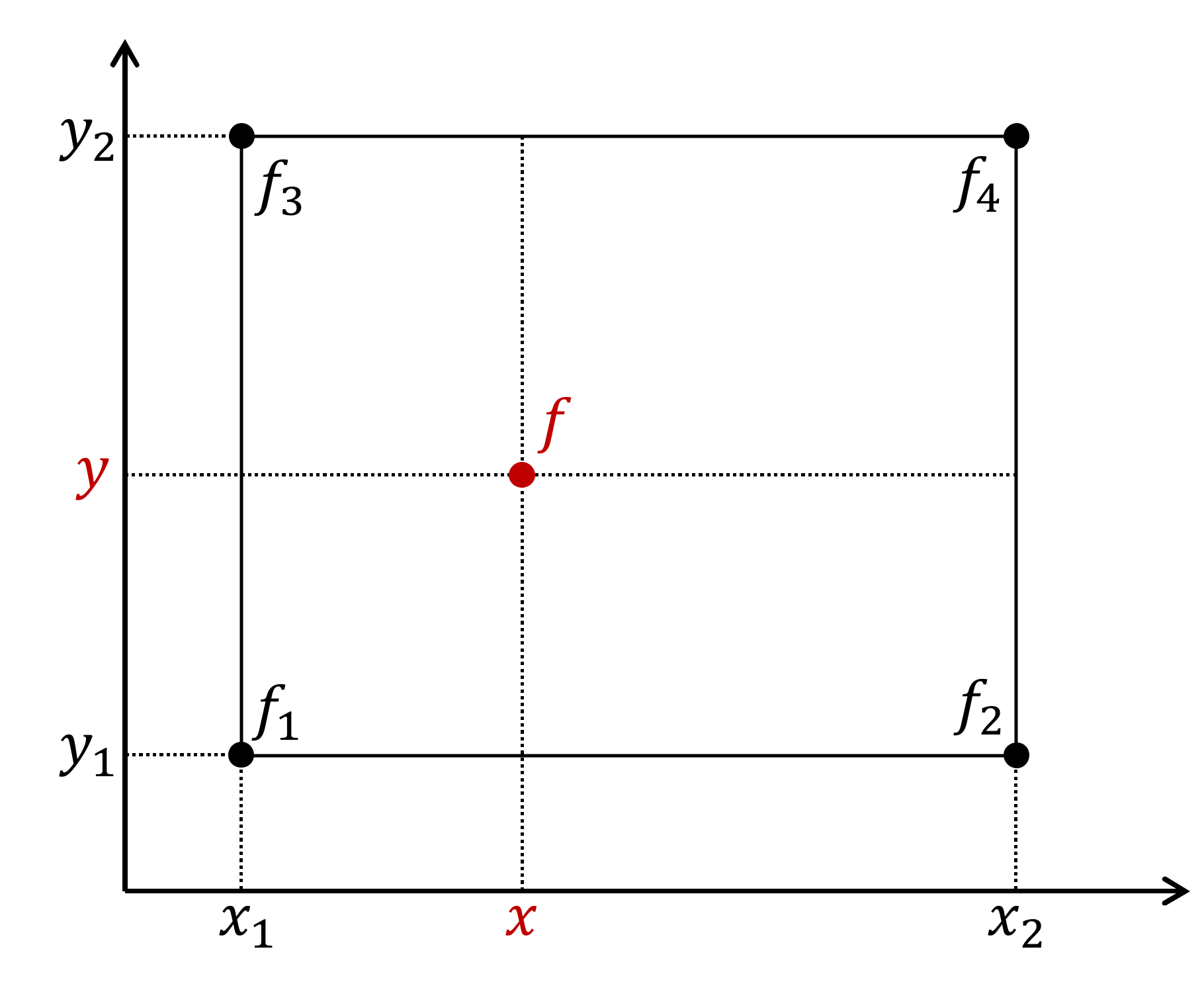
Figure 1 shows the configuration of a target point on which conventional bilinear interpolation proceeds using the four rectangular points surrounding the target point. The procedure is simply linear interpolations, first along the x-axis and then along the y-axis. Centering the target point, weighting for the interpolation is given by the area ratio of the four rectangles to their area sum. This way of weighting is identical to the conventional bilinear interpolation method [4].

$$f\left(x,y\right)=w_1{f}_1+w_2{f}_2+w_3{f}_3+w_4{f}_4,$$

where

$$\begin{gathered} w_1=\frac{\left(x_2-x\right)\left(y_2-y\right)}{\left(x_2-x_1\right)\left(y_2-y_1\right)}, \\ {w}_2=\frac{\left(x-x_1\right)\left(y_2-y\right)}{\left(x_2-x_1\right)\left(y_2-y_1\right)}, \\ {w}_3=\frac{\left(x_2-x\right)\left(y-y_1\right)}{\left(x_2-x_1\right)\left(y_2-y_1\right)}, \\ {w}_4=\frac{\left(x-x_1\right)\left(y-y_1\right)}{\left(x_2-x_1\right)\left(y_2-y_1\right)}. \end{gathered}$$

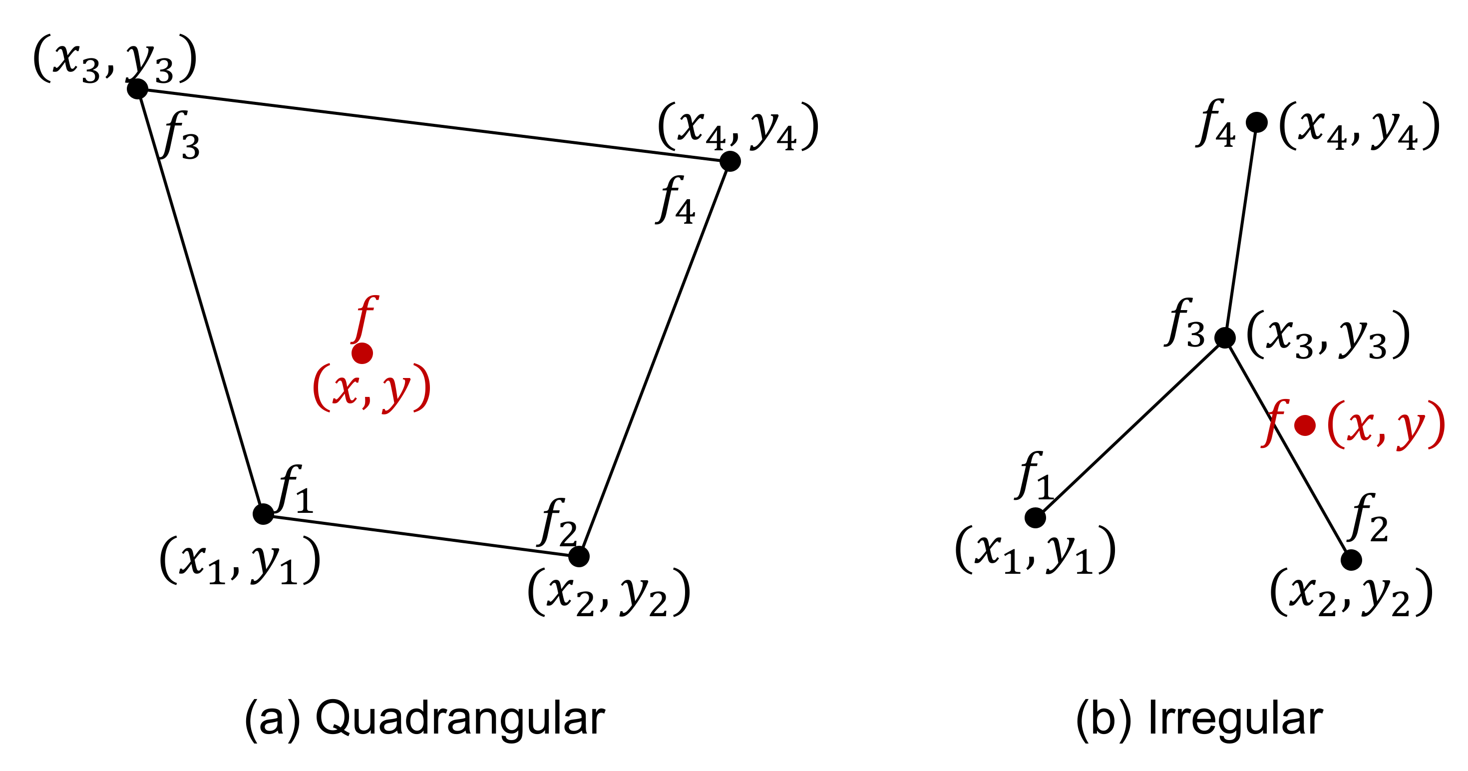
Meanwhile, Figure 2 exhibits examples of the bilinear interpolation on a target using four points which do not form a rectangle, and shows that the bilinear interpolation method as suggested in this study is applicable to any geometrical configuration of source points near a target point. Now, we explain this assumption and the idea behind the bilinear interpolation proposed in this study. The function for the interpolation is given by

$$f\left(x,y\right)=a+bx+cy+dxy.$$

The choice for the function is made on the basis that it is as simple as possible and is identical to conventional bilinear interpolation if the four source points form a rectangle. The coordinates of those four source points are denoted by $\left(x_1,y_1\right)$, $\left(x_2,y_2\right)$, $\left(x_3,y_3\right)$, and $\left(x_4,y_4\right)$, and their corresponding function values are $f_1$, $f_2$, $f_3$, and $f_4$, respectively. A system of equations can be formed and expressed as the multiplication of a matrix and a vector:

$$\left[\begin{array}{cccc}1& x_1& y_1& x_1{y}_1\\ 1& x_2& y_2& x_2{y}_2\\ 1& x_3& y_3& x_3{y}_3\\ 1& x_4& y_4& x_4{y}_4\end{array}\right]\left[\begin{array}{c}a\\ b\\ c\\ d\end{array}\right]=\left[\begin{array}{c}{f}_1\\ f_2\\ f_3\\ f_4\end{array}\right].$$

Once the system of equations has been solved, the coefficients $a$, $b$, $c$, and $d$ of the corresponding function can be obtained, and the bilinear interpolation of the function f(x, y) on the position of any arbitrary point near those four points can proceed. In particular, the following two key points should be examined to ensure that the accuracy of the interpolation is acceptably equivalent to that of conventional bilinear interpolation.

(1) We need to seek a 4 × 4 matrix whose determinant becomes maximum by rotating the x–y axes of the four source points to obtain relevant coordinates to the interpolation. In other words, the accuracy of this bilinear interpolation process depends upon the coordinates of the chosen four neighboring points. According to Cramer’s rule (Apostol, 1969) for a system of equations, coefficients can be given by the ratios of determinants $D_1$, $D_2$, $D_3$, and $D_4$ and to the determinant $D$, where they are defined as follows:

$$D=\left|\begin{array}{cccc}1& x_1& y_1& x_1{y}_1\\ 1& x_2& y_2& x_2{y}_2\\ 1& x_3& y_3& x_3{y}_3\\ 1& x_4& y_4& x_4{y}_4\end{array}\right|,$$

$$D_1=\left|\begin{array}{cccc}{f}_1& x_1& y_1& x_1{y}_1\\ f_2& x_2& y_2& x_2{y}_2\\ f_3& x_3& y_3& x_3{y}_3\\ f_4& x_4& y_4& x_4{y}_4\end{array}\right|,D_2=\left|\begin{array}{cccc}1& f_1& y_1& x_1{y}_1\\ 1& f_2& y_2& x_2{y}_2\\ 1& f_3& y_3& x_3{y}_3\\ 1& f_4& y_4& x_4{y}_4\end{array}\right|,$$

$$D_3=\left|\begin{array}{cccc}1& x_1& f_1& x_1{y}_1\\ 1& x_2& f_2& x_2{y}_2\\ 1& x_3& f_3& x_3{y}_3\\ 1& x_4& f_4& x_4{y}_4\end{array}\right|,D_4=\left|\begin{array}{cccc}1& x_1& y_1& f_1\\ 1& x_2& y_2& f_2\\ 1& x_3& y_3& f_3\\ 1& x_4& y_4& f_4\end{array}\right|.$$

Subsequently, the coefficients in the system of equations can be given as:

$$a=\frac{D_1}{D},b=\frac{D_2}{D},c=\frac{D_3}{D},d=\frac{D_4}{D}.$$

For example, let us consider a rotation matrix transformed with respect to the origin and with the angle $\theta$ from the original matrix given the target point and the four aforementioned neighboring points. After this, the determinants $D$ and $D_4$ become

$$D=\mathrm{A}\cos 2\theta +B\sin 2\theta =A\prime \cos (2\theta -\varphi ),\mathrm{where}\cos \varphi =\frac{B}{A^2+B^2},$$

$$\begin{array}{ll}A=& -(x_1{x}_2+x_3{x}_4)(y_1-y_2)(y_3-y_4)\\ & +(x_1{x}_3+x_2{x}_4)(y_1-y_3)(y_2-y_4)\\ & -(x_1{x}_4+x_2{x}_3)(y_1-y_4)(y_2-y_3)\end{array}$$

$$\begin{array}{ll}2B=& -(x_1{x}_2+y_3{y}_4)(x_1-x_2)(y_3-y_4)+(x_1{x}_3+y_2{y}_4)(x_1-x_3)(y_2-y_4)\\ & -(x_1{x}_4+y_2{y}_3)(x_1-x_4)(y_2-y_3)-(x_2{x}_3+y_1{y}_4)(x_2-x_3)(y_1-y_4)\\ & +(x_2{x}_4+y_1{y}_3)(x_2-x_4)(y_1-y_3)-(x_3{x}_4+y_1{y}_2)(x_3-x_4)(y_1-y_2)\end{array}$$

$$\begin{array}{ll}{D}_4=& -(f_1{x}_2-f_2{x}_1)(y_3-y_4)+(f_1{x}_3-f_3{x}_1)(y_2-y_4)-(f_1{x}_4-f_4{x}_1)(y_2-y_3)\\ & -(f_2{x}_3+f_3{x}_2)(y_1-y_4)+(f_2{x}_4-f_4{x}_2)(y_1-y_3)-(f_3{x}_4-f_4{x}_3)(y_1-y_2)\end{array}$$

Here, $D_4$ is independent of the coordinates' change of the four source points so that the coefficient becomes minimal when we rotate the axes of source points in such a way that the determinant becomes maximal. The accuracy of the interpolation is mainly affected by the coefficient $d$ in that the accuracy is highest when $d$ is minimum, i.e., when $D$ is maximum. Geometrically, the function appears as flat when $d$ is minimum.

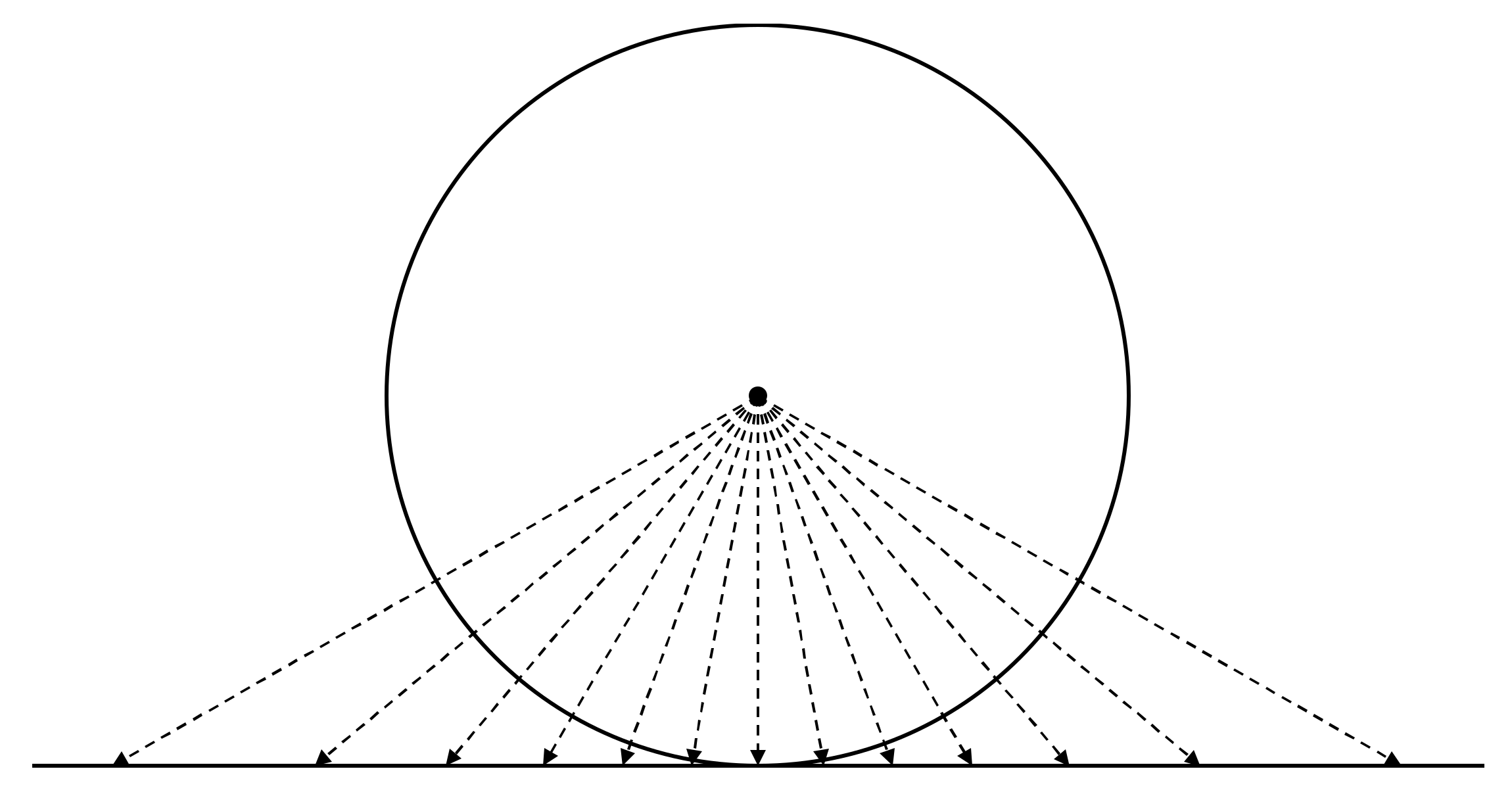
(2) Another key point for accuracy is to ensure that more than three out of the four source points neighboring the target point for the interpolation should not be in a line because if this is the case, the determinant D of the matrix becomes zero, which cannot be used for the interpolation. In practice, if three out of the four points are in a line, this configuration leads to low interpolation accuracy even though the determinant is not zero. We discovered this from our experience with various interpolation experiments; in any case, we note that the bilinear polynomial can actually degenerate into a linear one in such situations, even if the interpolation data come from a quadratic (or higher degree) polynomial. This bilinear interpolation method employs two-dimensional space to execute the interpolation of quantities over any spherical grid, thus there is a requirement that spherical points should be projected on a two-dimensional plane. In this study, we use the gnomonic projection as we think that the interpolation accuracy is not sensitive to the choice of projection. Figure 3 shows the gnomonic projection of points on a sphere on a 2-dimensional plane. In this situation, the length between the points and the area surrounding them become more distorted as the target point is moved further away from the center. To minimize such distortion through conventional gnomonic projection, we employ the latter in such way that the target point is always centered.

3. The Search Algorithm

One of the core processes for the proposed bilinear interpolation method is to find the four nearest source points to the target point. To apply this even for randomly distributed points on a sphere, we designed the method to require only the latitude–longitude coordinates of those points as input information. The distances between the target and source points need to be computed, and in general, this demands a computational cost proportional to $N^2$, and so we applied a linked-cell mapping method for the search, which reduces it proportional to $N\mathit{log}N$.

The linked-cell or cell linked list method [10] is frequently used in the studies of molecular dynamics and has been applied to the search for interacting particles depending on their distances from the target particle. It is an efficient tool that enables searching by storing particles in rectangular cells uniformly divided in space and considering particles only in the same cell where the target point is located. This method leads to a reduction in the computational cost for simulations of molecular dynamics overall by calculating interactions only within a cell. In general, a variable array is used as a linked list for the method, but we use a fixed array for the search list in this study similar to the method introduced in [11]. This provides a fixed size of the array for the list, which is another computational advantage for the search.

To enable the linked-cell mapping method to function effectively on a sphere, we use the cubed-sphere grid as a reference frame, since sizes of the elements on the cubed-sphere do not vary by much and it is easy to find neighboring elements [12]. Figure 4 shows the distribution of elements on the cubed-sphere as a reference frame for the search of source points using the linked-cell mapping method. We show an example of a search using 50 × 25 latitude–longitude grid points and a cubed-sphere with 10 × 10 elements in each panel. Now, we explain the concept of linked-cell mapping by taking the area colored red in Figure 4 into account. The procedure is as follows:

• Information in two index arrays is required: cube_links (ne,ne,6) providing the information of indices of the elements on the cubed-sphere and grid_links (grid_size) containing the indices of the latitude–longitude grid points linked to the specific elements in cube_links (ne,ne,6).
• The coordinates of the latitude–longitude grid points $\left(\lambda ,\theta \right)$ are then transformed into the coordinates of $\left(\alpha ,\beta ,panel\right)$ on the cubed-sphere, and the index of each element containing the transformed coordinates (corresponding to ei = 8, ej = 7, and panel = 6 in Figure 4) is identified.
• Among the indices of the three transformed grid points, the smallest index is 1067, thus we assign cube_links (8,7,6) = 1067 and grid_links (1067) = −1.
• The second index on the mapping list is 1068, and we replace cube_links (8,7,6) = 1068 with grid_links (1067) = −1 while grid_links (1068) = 1067.
• This is repeated for the third index of the mapping: cube_links (8,7,6) = 1069 and then grid_links (1067) = −1, grid_links (1068) = 1067, and grid_links (1069) = 1068.
• Subsequently, the search of points corresponding to element (8,7,6) starts with the saved information cube_links (8,7,6) = 1069 and checks the values of grid_links (1069) = 1068 until −1 is returned for “grid_links” as follows:
  cube_links (8,7,6) = 1069 → grid_links (1069) = 1068 → grid_links (1068) = 1067 → grid_links (1067) = −1

Now, we explain the search procedure of neighboring points for the proposed bilinear interpolation using the cubed-sphere as a reference frame (Figure 4). We assume that the latitude–longitude grid points are transformed on the cubed-sphere and the two index arrays of the linked-cell mapping are prepared as described in the previous paragraph.

• Next, we identify the element that contains the given target point, which is denoted by the x-mark (the yellow-colored element in Figure 4). Using the linked-cell mapping method, we search the source points mapped in that element.
• If the number of source points is less than 4, as in the yellow-colored element in Figure 4, source points mapped in the seven elements surrounding that element are included in the search (the cyan-colored elements in Figure 4).
• The search proceeds in the expanded area unless enough source points are sought (the green-colored elements in Figure 4).
• If more than four source points are available, then they are classified according to their distances from the target point.
• From the four closest points, we examine whether they satisfy the following conditions. A set of four source points that passes those conditions is then selected.

  -

  The determinant, D ≠ 0 (If D = 0, then the source points can be duplicated).

  -

  For accuracy, three of the four points should not be in a line.

• Finally, using the selected set of four source points, we conduct the bilinear interpolation.

4. Experiments

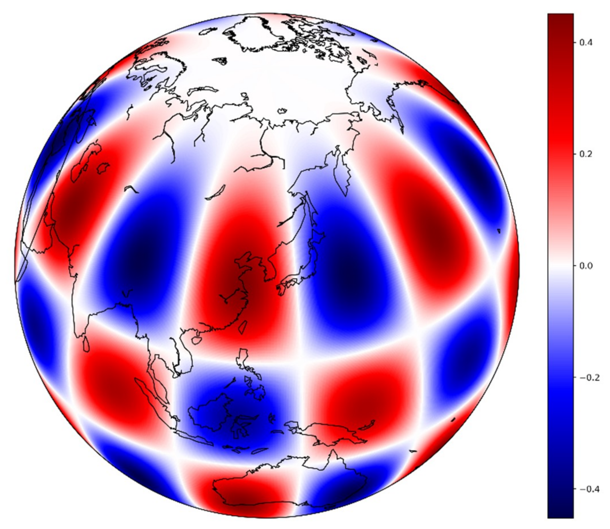
Figure 5 shows the four chosen grid systems on the sphere for the verification of our bilinear interpolation method. We chose a latitude–longitude grid, a cubed-sphere, a Fibonacci sphere, and randomly distributed points scattered on a sphere, and the accuracy of the bilinear interpolation of a given test function was used for the comparison. Figure 6 shows the given test function for the experiment consisting of spherical harmonics $Y_l^m$, where l = 8 and m = 6.

The set of metrics for the comparison includes relative error norms L₁, L₂, and L_∞:

$$\begin{gathered} L_1=\frac{{{\displaystyle \sum }}_i{\left|f_{remap}-f_{ref}\right|}_i}{{{\displaystyle \sum }}_i{\left|f_{ref}\right|}_i} \\ {L}_2=\frac{\sqrt{{{\displaystyle \sum }}_i{(f_{remap}-f_{ref})}_i^2}}{\sqrt{{{\displaystyle \sum }}_i{(f_{ref})}_i^2}} \\ {L}_{\infty }=\frac{\mathit{max}({\left|f_{remap}-f_{ref}\right|}_i)}{\mathit{max}({\left|f_{ref}\right|}_i)} \end{gathered}$$

There were two groups of experiments: the conventional bilinear interpolation test and the proposed bilinear interpolation test.

In the first group, there were again two sets of remapping tests: (1) we remapped from the latitude–longitude grid system to the other grid systems using equirectangular projection and rectangular bilinear interpolation, and (2) we remapped from the cubed-sphere to the other grid systems using fixed gnomonic projection and rectangular bilinear interpolation.

In the second test group, we experimented with our alternative bilinear interpolation method using variable gnomonic projection and interpolation including non-logically rectangular points on the sphere: (1) from the latitude–longitude grids to the other grid systems, (2) from the cubed-sphere to the other grid systems, (3) from the Fibonacci sphere to the other grid systems, and (4) from the randomly distributed points to the other grid systems.

Table 1. Relative error norms from the remapping experiments between the different spherical grid point systems.

	Latlon Rectangle			Cube Rectangle			General 4 Points
	L1	L2	Linf	L1	L2	Linf	L1	L2	Linf
latlon->cube	1.47E-03	1.59E-03	2.25E-03	N/A			1.47E-03	1.59E-03	2.25E-02
latlon->fibonacci	1.46E-03	1.58E-03	2.27E-03				1.44E-03	1.56E-03	2.24E-03
latlon->random	1.41E-03	1.54E-03	2.27E-03				1.40E-03	1.54E-03	2.27E-03
cube->latlon	N/A			2.09E-03	2.29E-03	4.64E-03	1.92E-03	2.11E-03	4.61E-03
cube->fibonacci				2.08E-03	2.27E-03	4.54E-03	1.88E-03	2.09E-03	7.40E-03
cube->random				2.09E-03	2.28E-03	4.52E-03	1.92E-03	2.11E-03	4.51E-03
fibonacci->cube	N/A			N/A			1.72E-03	1.76E-03	2.34E-03
fibonacci->latlon							1.72E-03	1.76E-03	2.43E-03
fibonacci->random							1.73E-03	1.77E-03	2.33E-03
random->cube	N/A			N/A			4.08E-03	6.15E-03	1.31E-01
random->latlon							3.94E-03	5.85E-03	1.05E-01
random->fibonacci							4.09E-03	6.11E-03	9.68E-02

contains a list of the relative error norms (L₁, L₂, and $L_{\infty }$) for each test. This shows that there were only minor differences in interpolation accuracy between the remapping in the control and test groups. For the remapping from the cubed-sphere to the other grid systems, the accuracy was slightly improved by using variable gnomonic projection and the alternative bilinear interpolation method. This might have resulted from the fact that the latter is free from the constraint of rectangular source points surrounding a target point, thus we could use source points located closer to the target point. A similar accuracy was obtained in the proposed bilinear interpolation of the Fibonacci sphere and the random points of the other grid systems.

Meanwhile, the randomly distributed points became denser as the latitude increased, and overall accuracy might have depended more on the intervals between the points at lower latitudes. Therefore, a large L_∞ error rate resulted from situations where the points lay far away from each other. Nevertheless, the order of error norms L₁ and L₂ remained as O (${10}^{-3}$), which demonstrates that the alternative bilinear interpolation method was useful even for randomly distributed points on a sphere.

Figure 7 shows the computational time for the alternative bilinear interpolation with an increasing number of grid points N, which shows that the computational time is proportional to $N\mathit{log}N$, instead of $N^2$. Moreover, the computational cost for the linked-cell mapping was nearly proportional to N instead of $N\mathit{log}N$ since the search for neighboring points was able to proceed without considering all of the grid points, only the four nearest ones instead. The number of grid points in our tests ranged from 48,602 ~ 12,441,602. We used a single core with a single thread from an Intel Xeon CPU E5-2690 2.90 GHz; the Fortran compiler used was gfortran v4.7.1.

5. Conclusions

In this study, we suggest an alternative bilinear interpolation method for remapping between spherical grids, even for randomly distributed points on a sphere. One of the key ideas behind this method is that the interpolation function is derived from a system of equations for four source points regardless of their geometrical configuration with respect to a target point. The system of equations can be represented in a 4 × 4 matrix-vector multiplication form and elements of the matrix are chosen in such way that the determinant is maximized through the rotation of the coordinate system for the four source points. This is an essential property of the alternative bilinear interpolation method, which makes the method applicable for any spherical grid system.

Another key idea is the combination of the linked-cell mapping method for an efficient search of neighboring source points and the cubed-sphere as a reference frame for convenience when searching. This results in a computational cost proportional to $N\mathit{log}N$ instead of $N^2$, even for the remapping of randomly distributed points on a sphere.

For the verification of the proposed bilinear interpolation, we compared the remapping accuracy of a spherical harmonic function with conventional bilinear interpolation available for logically rectangular grids. In addition, we examined the feasibility of the alternative bilinear interpolation method for diverse grid systems on a sphere. The results show that our bilinear interpolation method provided an equivalent remapping accuracy to the conventional bilinear interpolation one. The computational cost measured in the test using this alternative bilinear interpolation method was proportional to $N\mathit{log}N$ instead of N², thus the method is applicable even for high-resolution interpolation.

However, there are two limitations to the interpolation method proposed in this study. The first one is the limited interpolation accuracy compared to what can be achieved by higher-order interpolation methods like radial basis function interpolation. The second one is that the bilinear interpolation cannot guarantee monotonicity, and so conservative remapping would be required for quantities like fluxes and precipitation. Besides, in our study we have solved the problem of the aligned three points in such a way as to find a new candidate point, but it can be also solved by using the least square fitting. Another way is to identify the optimal configuration of points using an approach such as the study of the remainder of the bilinear polynomial interpolant in a special form [13,14]. Regarding to the accuracy and efficiency of the method, we will examine also these issues in our future studies. Nevertheless, the alternative bilinear interpolation method is still useful in diverse geoscientific investigations due to the relatively low computational cost and the ease of implementation. Moreover, the method suggested in this study is applicable to any spherical grid system, even if they are not logically rectangular. This method can also achieve reasonable interpolation accuracy even for randomly distributed points on a sphere and is feasible for high-resolution remapping due to its relatively low computational cost.

References

- Sadourny, R. Conservative finite-difference approximations of the primitive equations on quasi-uniform spherical grids. Mon. Weather Rev. 1972, 100, 136–144. [Google Scholar] [CrossRef]
- Heikes, R.; Randall, D.A. Numerical integrations of shallow-water equations on a twisted icosahedral grid. Part I: Basic design and results. Mon. Weather Rev 1995, 123, 1862–1880. [Google Scholar] [CrossRef]
- Hill, C.; Deluga, C.; Balaji, V.; Suarez, M.; da Silva, A. The architecture of the earth system modeling framework. Comput. Sci. Eng. 2004, 6, 18–28. [Google Scholar] [CrossRef]
- Press, W.H.; Teukolsky, S.A.; Vetterling, W.T.; Flannery, B.P. Numerical Recipes in C—The Art of Scientific Computing, 2nd ed.; Cambridge University Press: New York, NY, USA, 1992. [Google Scholar]
- Jones, P.W. First- and second-order conservative remapping. Mon. Weather Rev. 1999, 127, 2204–2210. [Google Scholar] [CrossRef]
- Ullrich, P.A.; Lauritzen, P.H.; Jablonowski, C. Geometrically exact conservative Remapping (GECoRe): Regular latitude–longitude and cubed-sphere grids. Mon. Weather Rev. 2009, 137, 1721–1741. [Google Scholar] [CrossRef]
- Khoei, A.R.; Gharehbaghi, S.A. The superconvergent patch recovery technique and data transfer operators in 3d plasticity problems. Finite Elem. Anal. Des. 2007, 43, 630–648. [Google Scholar] [CrossRef]
- Jones, P.W. A User’s Guide for SCRIP Version 1.5; Los Alamos National Laboratory, University of California: Oakland, CA, USA, 1998. [Google Scholar]
- Balaji, V.; Boville, B.; Cheung, S.; Clune, T.; Collins, N.; Craig, T.; Cruz, C.; da Silva, A.; DeLuca, C.; de Fainchtein, R.; et al. ESMF Reference Manual for Fortran Version 7.1.0r, 208. Available online: http://www.earthsystemmodeling.org/esmf_releases/public/ESMF_7_1_0r/ESMF_refdoc/ESMF_refdoc.html (accessed on 8 March 2018).
- Allen, M.P.; Tildesley, D.J. Computer Simulation of Liquids; Clarendon Press: Oxford, UK, 1987. [Google Scholar]
- Rapport, D.C. Large-scale molecular dynamics simulation using vector and parallel computers. Comput. Phys. Rep. 1988, 9, 1–53. [Google Scholar] [CrossRef]
- Kim, K.-H.; Shim, P.; Shin, S. A simple method to find a neighboring grid point on the cubed-sphere. Asia-Paci. J. Atmos. Sci. 2018, 54, 413–419. [Google Scholar] [CrossRef]
- Dell’Accio, F.; di Tommaso, F.; Hormann, K. On the approximation order of triangular Shepard interpolation. IMA J. Numer. Anal. 2016, 36, 359–379. [Google Scholar] [CrossRef]
- Dell’Accio, F.; di Tommaso, F.; Nouisser, O.; Zerroudi, B. Increasing the approximation order of the triangular Shepard method. Appl. Numer. Math. 2018, 126, 78–91. [Google Scholar] [CrossRef]
Figure 1.
An example of bilinear interpolation for function f on position (x, y) in a rectangular constellation formed by four grid points , , , and using their corresponding functions , , , and .
Figure 2.
Examples of the alternative bilinear interpolation for function f on position (x, y): (a) quadrangular and (b) irregular constellations of four grid points , , , and using their corresponding functions , , , and .
Figure 3.
A gnomonic projection showing the increase of distortion as the target of the projection is further from the center.
Figure 4.
Linked-cell mapping with the cubed-sphere elements: latitude–longitude grid points (50 × 25 resolution) are mapped to the cubed-sphere elements (ne10 resolution).
Figure 5.
The spherical grid systems investigated in this study: (a) latitude–longitude, (b) cubed-sphere, (c) Fibonacci sphere, and (d) random points.
Figure 6.
The test function used in this study: spherical harmonics .
Figure 7.
The wall clock times for the remapping experiments with increasing grid resolution.