Short-Range Numerical Weather Prediction of Extreme Precipitation Events Using Enhanced Surface Data Assimilation

Abstract

A limited-area kilometre scale numerical weather prediction system is applied to evaluate the effect of refined surface data assimilation on short-range heavy precipitation forecasts. The refinements include a spatially dependent background error representation, use of a flow-dependent data assimilation technique, and use of data from a satellite-based scatterometer instrument. The effect of the enhancements on short-term prediction of intense precipitation events is confirmed through a number of case studies. Verification scores and subjective evaluation of one particular case points at a clear impact of the enhanced surface data assimilation on short-range heavy precipitation forecasts and suggest that it also tends to slightly improve them. Although this is not strictly statistically demonstrated, it is consistent with the expectation that a better surface state should improve rainfall forecasts.

1. Background

Numerical weather prediction (NWP) is concerned with, starting from an initial state, integrating the atmospheric state forward in time. The atmospheric state is represented by a number of variables defined on discrete grid points, and the model is run forward in time to simulate the atmosphere and its evolution. Some processes take place on scales that cannot be represented by the model and are accounted for through various parametrizations. Data assimilation in NWP optimally blends observations with a forecast from the atmospheric model in order to obtain the spatial distribution of atmospheric variables and to produce the best possible model initial state. It was early realised that the forecast quality is strongly dependent on an accurate description of the initial state and, hence, on the capability of the assimilation system [1].

Surface processes, such as heat and water exchanges, are essential to represent in NWP. The present study was carried out within the European Union’s Horizon 2020 project IMPREX (IMproving PRedictions and management of hydrological EXtremes) where the ambition is to enhance forecast quality of extreme hydrometeorological conditions and their impacts. The current work is an extension based on project developments and results by Lindskog and Landelius [2]. Here, we improve the handling of surface quantities and focus on the effect on short-range (days ahead) weather forecasting. Refined surface data assimilation in NWP has the potential to result in an improved prediction of severe precipitation events. Impact of of soil moisture conditions on short- and medium-range NWP have earlier been demonstrated [3,4,5,6,7,8]. In addition, the importance of an accurate soil moisture representation has also been demonstrated at the seasonal range [9,10,11].

Here, we use the HARMONIE-AROME NWP system [12], which is one configuration of the shared Aire Limitée Adaptation Dynamique Developpement InterNational (ALADIN)-High-Resolution Limited-Area Model (HIRLAM) NWP system. The HARMONIE-AROME system is comprised of a data assimilation system for the surface and upper-air together with a forecast model.

Our aim is to improve short-range NWP of extreme precipitation by enhancing the representation of the surface initial state by applying an improved HARMONIE-AROME surface data assimilation. The enhancements concern both methodologies in data assimilation and enhanced observation usage. Situation-dependent background error statistics is introduced. and horizontal small-scale variations are better represented. In addition, use of scatterometer soil moisture-related data has been introduced. One or two of these improvements have been applied before in research and to operational systems [8,13,14,15,16]. Here, we combine these enhancements and merge them for the first time into one novel state-of-the-art data assimilation system. Three cases associated with heavy precipitation are used to get insight on the potential of these combined enhancements. The weather situations include both large-scale, orographically forced precipitation events and also convective events over flat land.

The components of the HARMONIE-AROME forecasting system are the subject of Section 2, with focus on surface data assimilation. In Section 3, the model configuration and the heavy precipitation cases are described. Section 4 is concerned with an investigation of the abilities of the enhanced NWP system. Experimental setup is the subject of Section 5, followed by the associated findings in Section 6. Conclusions are emphasised in Section 7.

2. The Forecasting System and Surface Initial State

2.1. NWP System

The HARMONIE-AROME modelling configuration is comprised of a data assimilation system and a forecast model. The data assimilation consists of two parts, which cover respectively the surface and upper-air. A detailed description of the forecast model setup is given in Seity et al. [17] and Bengtsson [12]. It is a non-hydrostatic model formulation with a spectral representation of the model state. The Eddy Diffusivity Mass Flux (EDMF) scheme is used for sub-grid cloud parametrization. Turbulence processes are represented according to Cuxart et al. [18]. The radiative transfer is modelled as described by Fouquart and Bonnel [19] and Mlawer et al. [20] for short- and long-wave radiation processes, respectively. For surface processes, the SURFEX (Surface Externalisée) scheme [21] is employed together with an ISBA (interactions between the soil–biosphere–atmosphere) scheme [22,23] that uses a force-restore method [24]. The version of the scheme used here has two vertical temperature layers and three layers for soil moisture [25]. The third and deepest soil moisture level was introduced to distinguish between the root zone and sub-root zone soil water reservoirs.

Global forecasts provided by the European Centre for Medium-Range Weather Forecasts (ECMWF) were used as lateral boundary conditions. These forecasts are launched every 6 h with a 1-h output frequency. Global model information was also used to replace larger-scale information in the background state with lateral boundary information [26]. The purpose of this is to make use of high-quality larger scale information in the ECMWF global fields.

Upper-air data assimilation is based on a 3-dimensional variational approach [27]. Types of observations that were assimilated include in situ measurements (pilot–balloon wind, radiosonde, aircraft, buoy, ship, and synop) and microwave radiances from various satellite-based instruments. Statistics for the background state are based on a climatological assumption and are calculated from an ensemble of forecast differences by downscaling global ECMWF ensemble forecasts over the limited-area. Scaling is applied to the derived statistics in order to be in agreement with the amplitude of HARMONIE-AROME + 3-h forecast errors.

2.2. Default Surface Data Assimilation of Temperature and Moisture

The HARMONIE-AROME reference surface data assimilation of temperature and moisture is comprised of two steps. In step one, a horizontal data assimilation based on the CANARI (Code d’Analyse Nećessaire á ARPEGE pour ses Rejets et son Initialisation) optimal interpolation scheme [28] is applied in two dimensions to horizontally spread the information from screen-level (two-metre) temperature and relative humidity observations to update two-metre temperature and relative humidity values over all land surface grid-points containing land parts. This is done according to the following equation:

$${\mathbf{x}}_a={\mathbf{x}}_b+\mathbf{B}{\mathbf{H}}^T{(\mathbf{H}\mathbf{B}{\mathbf{H}}^T+\mathbf{R})}^{-1}(\mathbf{y}-\mathbf{H}{\mathbf{x}}_b).$$

(1)

where ${\mathbf{x}}_a$ denotes the analysed values, ${\mathbf{x}}_b$ denotes the background values, and $\mathbf{y}$ denotes the observations. Furthermore, $\mathbf{B}$ is a matrix containing the background errors and $\mathbf{R}$ is a matrix containing the observation errors. $\mathbf{H}$ is the Jacobian of the observation operator. $\mathbf{R}$ is set to a diagonal matrix while $\mathbf{B}$ is assumed to be non-diagonal but isotropic and horizontally homogeneous with the following correlation function:

$$cor{r}_{i,j}=e^{-\frac{r_{i,j}}{2a}}.$$

(2)

Here, $cor{r}_{i,j}$ denotes the horizontal background error correlation between points i and j separated by $r_{i,j}$. The parameter a, which is the correlation length scale, was set to 80 km for temperature and 85 km for humidity. The background error standard deviations for temperature and relative humidity were assumed to be 1.6 K and 18%, respectively. The corresponding observation error standard deviations were assumed to be 1.4 K and 10%. The correlation functions are sometimes denoted structure functions. All these settings are carried over from the operational HARMONIE-AROME system.

In step two, after the two-dimensional horizontal distribution just described, the two-metre temperature and relative humidity information is vertically distributed to update the surface-soil model. This is done by the application of another optimal interpolation scheme as described in Equations (3)–(6), which originates from Equations (4)–(7) in Mahfouf et al. [13]. The procedure is applied independently for each grid-point, using the horizontally distributed two-metre temperature and relative humidity information to update the temperature and moisture in the soil layers:

$$w_g^a=w_g^b+{\alpha }_1(T_{2m}^a-T_{2m}^b)+{\alpha }_2(R{H}_{2m}^a-R{H}_{2m}^b),$$

(3)

$$w_2^a=w_2^b+{\beta }_1(T_{2m}^a-T_{2m}^b)+{\beta }_2(R{H}_{2m}^a-R{H}_{2m}^b),$$

(4)

$$T_s^a=T_s^b+{\mu }_1(T_{2m}^a-T_{2m}^b)+{\mu }_2(R{H}_{2m}^a-R{H}_{2m}^b),$$

(5)

$$T_2^a=T_2^b+{\nu }_1(T_{2m}^a-T_{2m}^b)+{\nu }_2(R{H}_{2m}^a-R{H}_{2m}^b),$$

(6)

where $T_{2m}$ and $R{H}_{2m}$ denote two-metre temperature and relative humidity, respectively. $T_s$ and $w_g$ denote soil-top values, and $T_2$ and $w_2$ denote layer-two values of soil moisture and temperature. Here, superscript a and b represent analysed and background values, respectively. Note that analysed two-metre temperature and relative humidity values are available in all grid-points as a result of the horizontal optimal interpolation. Furthermore, the empirical coefficients or functions ${\alpha }_1$, ${\alpha }_2$, ${\beta }_1$, ${\beta }_2$, ${\mu }_1$, ${\mu }_2$, ${\nu }_1$, and ${\nu }_2$ are chosen as explained in Giard and Bazile [29] and Coiffier et al. [30], and accordingly, the coefficients ${\mu }_2$ and ${\nu }_2$ are set to zero. The third and deepest soil moisture layer is less coupled to screen level and scatterometer soil top layer moisture observations [31] and is, therefore, left untouched by the above procedure.

3. Modelling System Setup and Description of Cases

The limited-area kilometre scale forecasting system is applied over a domain covering a southern part of Europe, as is illustrated in Figure 1. The three cases with heavy precipitation took place in an area inside the blue circle. These cases are described in

Table 1. Description of extreme precipitation events studied with the HARMONIE-AROME modelling system.

Period	Charachteristics
20130612–20130619	Heavy precipitation in the Pyrenees.
20130721–20130728	Large convective precipitation amounts in northern continental Europe.
20140622–20140625	Severe precipitation case in the southwestern part of France.

. An illustration of one of the cases is given by the SEVIRI (Spinning Enhanced Visible and InfraRed Imager) instrument satellite data visualised in Figure 2.

The model grid consists of 768 × 648 horizontal points with a 2.5-km separation and 65 vertical levels. Data assimilation was carried out every third hour within an intermittent data assimilation cycle, and every sixth hour, a +48-h forecast was launched.

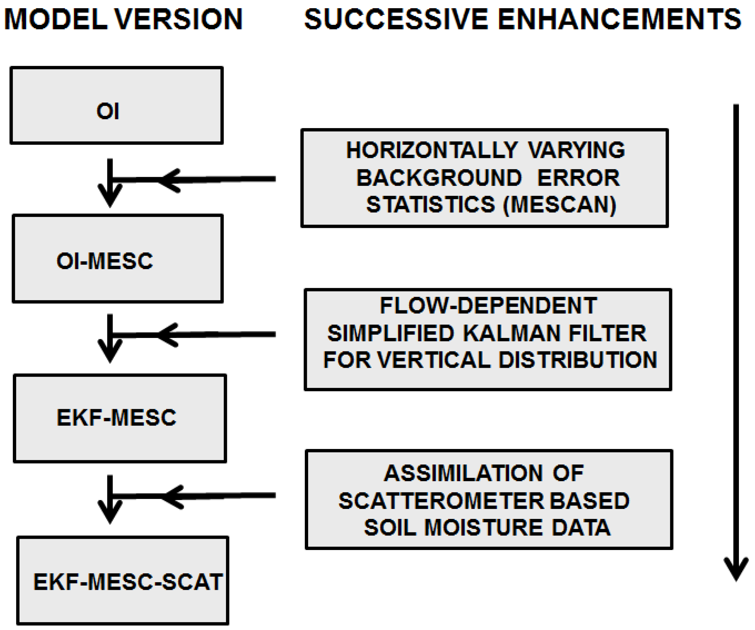
4. An Enhanced Assimilation of Surface Temperature and Soil Moisture

4.1. Overview

There are some obvious limitations in the reference surface data assimilation covered in Section 2. These are related to simplifying assumptions in the spatial distribution of observational information, to the lack of a proper flow-dependency, and to only using synoptic screen-level observations. With the refined system presented below, we have tried to alleviate these shortcomings.

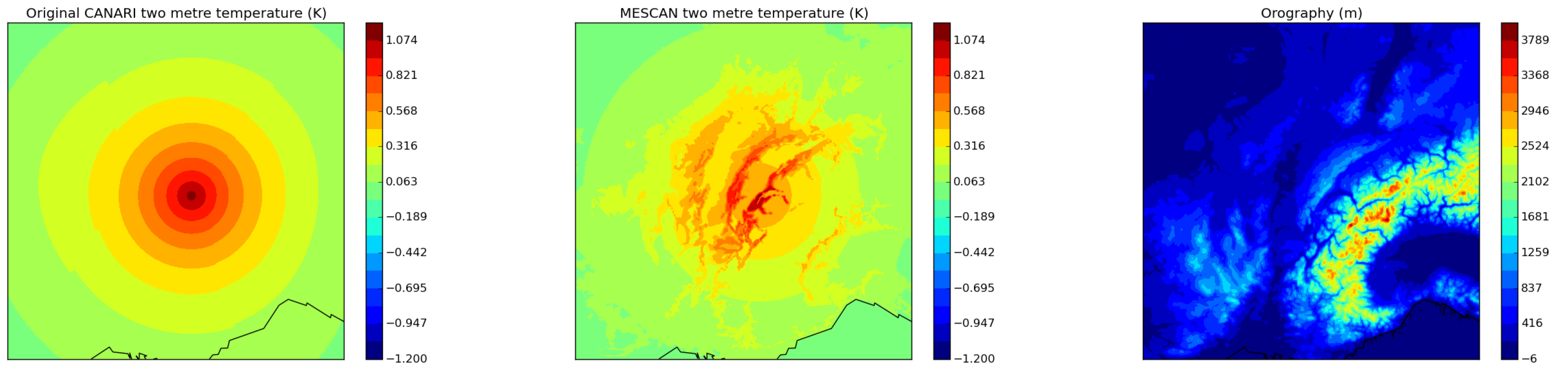
4.2. Screen-Level Structure Functions

The refined structure functions for two-metre temperature and humidity are based on developments made in the European FP7 project “European Reanalysis and Observations for Monitoring” (EURO4M). Here, the isotropic structure functions in the mesoscale analysis system CANARI were replaced with the orography-dependent ones used in MESAN, an operational mesoscale analysis system [32]:

$$corr(r_{i,j},d_p,d_z)=0.5[e^{-\frac{r_{i,j}}{L}}+(1+\frac{2r_{i,j}}{L})e^{-\frac{2r_{i,j}}{L}}]F_p\left(d_p\right)F_z\left(d_z\right).$$

(7)

The correlation difference due to land fraction ($dp$) and height ($dz$) between positions i and j and separated by a distance $r_{i,j}$ are represented by the linear functions $F_p$ and $F_z$. These are empirical scaling functions that describe a reduction of the correlation due to differences in fraction of land ($dp$) and height ($dz$) [32]. The function $F_p$ reduces the correlation with a factor of 0.5 when $dp=1$ and equals one when $dp=0$ (no reduction). In the same way, $F_z$ equals one when $dz=0$ and comes down to 0.5 when $dz$ exceeds 500 m. The correlation length scale, given by L in Equation (7), is set to 190 km for both variables.

This improved version of CANARI is known as MESCAN. Within the EURO4M project, the use of the anisotropic structure functions was shown to result in improved analyses of two-metre temperature and relative humidity [33,34]. In the present study, we relied on those results and assumed that our use of MESCAN would offer an improvement over CANARI when it comes to the horizontal surface screen-level analysis.

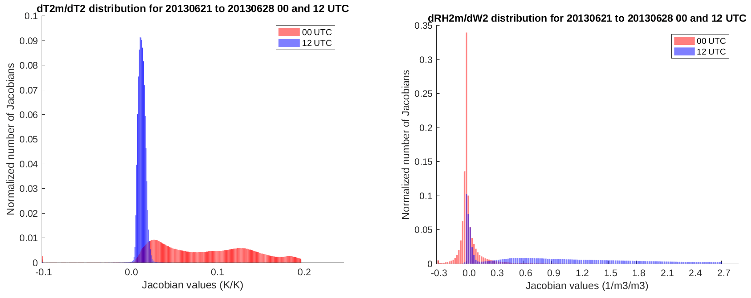
4.3. Flow-Dependent Vertical Spreading of Information

The refined vertical distribution of two-metre temperature and humidity information relies on a Kalman-filter approach. The analysed state is based on a methodology formally given by Equation (1) and with the Jacobian of the observation operator ${\mathbf{H}}_{i,j}$ approximated following Mahfouf et al. [13]. The approximation is obtained for each surface-soil data assimilation control variable (${\mathbf{x}}_j$) by performing one perturbed ($\delta {\mathbf{x}}_j$) model run and by projecting the results to observation space ${\mathbf{y}}_i$. This procedure is carried out for each analysis time every third hour and can formally be written as follows:

$${\mathbf{H}}_{i,j}=\frac{\partial {\mathbf{y}}_i}{\partial {\mathbf{x}}_j}\cong \frac{\partial {\mathbf{y}}_i(\mathbf{x}+\delta {\mathbf{x}}_j)-{\mathbf{y}}_i\left(\mathbf{x}\right)}{\delta {\mathbf{x}}_j}.$$

(8)

The main advantage, as compared to the reference system surface data assimilation procedure, is that it results in a flow-dependent coupling between observations and surface-soil control variables. Here, we have made the simplifying assumption that the background errors are uncorrelated and static. The latter assumption means that our improved methodology falls within the category Simplified Extended Kalman Filter (SEKF) as described by Draper et al. [35], where the flow-dependency of the SEKF enters through the Jacobians of the observation operator only and not through the $\mathbf{B}$ matrix.

Applying the denotations of Equations (3)–(6), the background error standard deviations applied in the vertical are 2.0 K for $T_2$ and $T_s$. For $w_2$ and $w_g$, the background error standard deviations used are 0.15 × ($w_{fc}-w_{wilt}$) and 0.1 × ($w_{fc}-w_{wilt}$), where $w_{fc}$ and $w_{wilt}$ are the volumetric water content at field capacity and at permanent wilting point, respectively, which depend on soil type [23]. The estimates of the observation error standard deviations are 1.0 K and 10% for gridded screen-level temperature and relative humidity, respectively. For scatterometer-based $w_g$, the observation error standard deviations is set to a value of 0.4 × ($w_{fc}-w_{wilt}$). The error estimates are based on Mahfouf el al. [13] and so are the values used in the perturbations of the control vector in the SEKF (${10}^{-4}$ for volumetric water content and ${10}^{-5}$ for temperature).

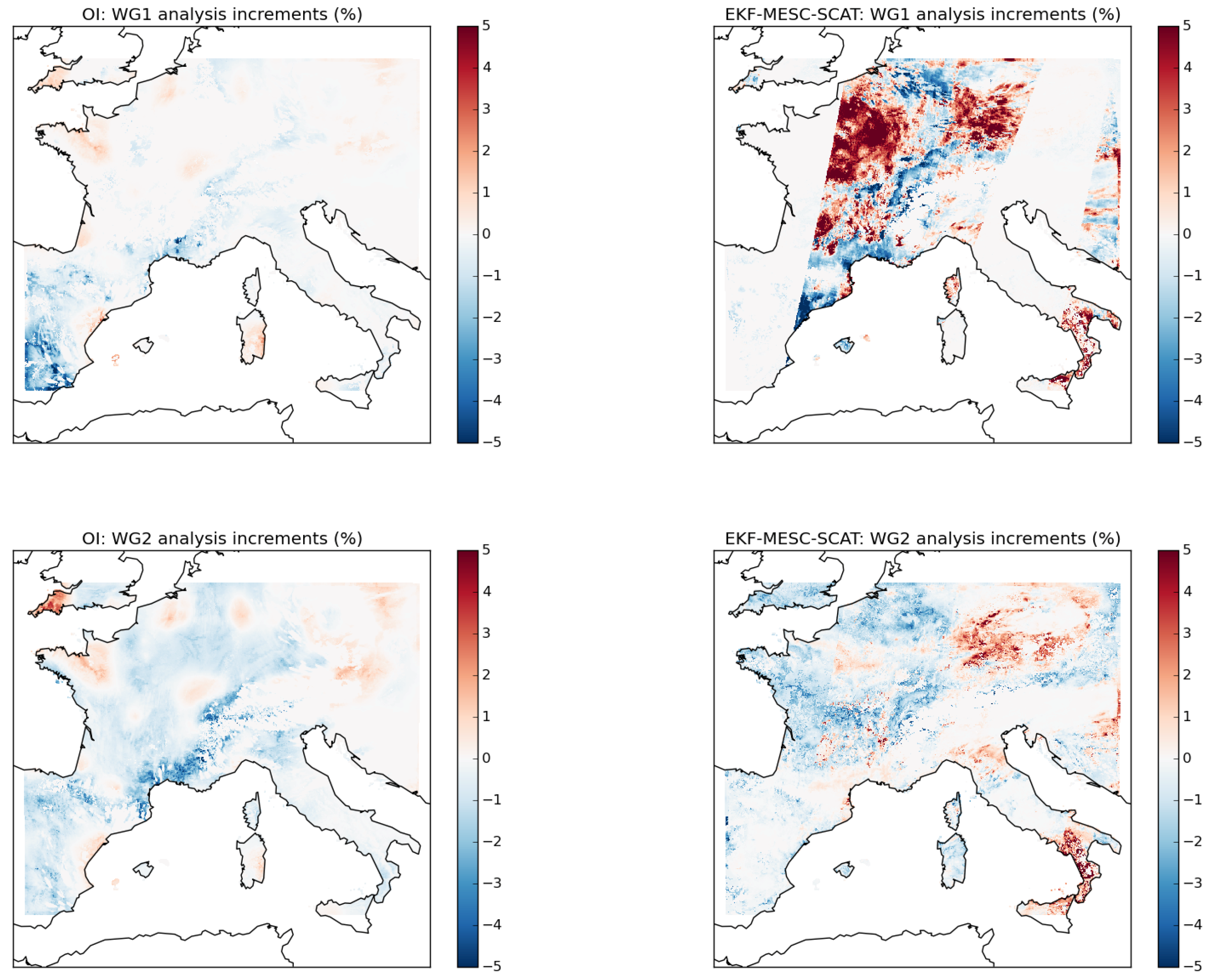
4.4. Use of Remote Sensing Data

There is a clear room for improvement regarding observation usage in the surface data assimilation in the reference system. In particular, the use of soil moisture data obtained from remote-sensing instruments is a promising next step of enhancement.

Use of satellite-based soil moisture products gives the potential to obtain an improved model soil moisture description through surface-soil data assimilation. The polar orbiting MetOp-A and MetOp-B satellites carry an Advanced SCATterometer (ASCAT) instrument, which can provide data related to soil moisture in the uppermost centimetres of the soil. The instrument is a radar backscatter instrument, and the horizontal resolution of the product used here is roughly 25 km [36].

A HARMONIE-AROME-specific preprocessing is applied to link the soil-top layer moisture product with the characteristics of the NWP model used. The pre-processing converts the scatterometer-based product, for which data is provided in degrees of saturation (ranging from 0% during dry conditions to 100% during wet conditions) to corresponding model moisture values. This processing is carried out separately for each model horizontal grid-point covered by an observation. Based on data from a two-month period, the maximum and minimum observed ASCAT soil-top layer moisture values ($ob{s}_{ascat}^{prodmax}$ and $ob{s}_{ascat}^{prodmin}$) were identified, as well as the corresponding maximum and minimum values in the top most level (one) of the soil model.

These estimates are then used to transform between the scatterometer product and the soil moisture in the top-most level of the surface-soil model ($w_g^{ascat}$). The transformation is then, at any given time, applied to all model grid-points covered by scatterometer data. The procedure is demonstrated in Figure 3 and can formally be described by the following equation:

$${\mathbf{w}}_g^{ascat}={\mathbf{w}}_g^{modmin}+\frac{w_g^{modmax}-w_g^{modmin}}{ob{s}_{ascat}^{prodmax}-ob{s}_{ascat}^{prodmin}}\times (ob{s}_{ascat}^{prod}-ob{s}_{ascat}^{prodmin}).$$

(9)

Here, the model value from the grid point og the nearest neighbour to the observation position is used. However, note that there is a significant difference in scales between the model data at 2.5 km and the ASCAT product at 25 km. This inconsistency should ideally be taken care of by having an observation operator that provides model equivalents at the same scale as the satellite observations, based on how the satellite antenna pattern interacts with the underlying model data.

The preprocessing is applied independently for the two different satellites. Since different satellite passages in general are associated with different spatial coverage, potential differences in characteristics between differences passages are accounted for through the conversion carried out separately for each horizontal position. Ideally, conversion between the scatterometer soil moisture product and model soil moisture should be based on a period long enough to build the statistics covering a wide range of plausible soil moisture states. The length of the time period used here was limited by practical constraints, such as available computing resources. In future operational use, the period could be extended by using archived model data. The above approach is similar to the cumulative distribution function (CDF) matching method proposed by Reichle et al. [37]. In the CDF case, each soil moisture time series is rescaled by subtracting the mean and by dividing by the standard deviation and then uses these normalized variables in the data assimilation. In the future, we will also investigate the effect of using such methods for relating the ASCAT product to the control variables in the data assimilation, as proposed by Dharssi et al. [38] and by de Rosnay et al. [31].

Ideally, the scatterometer soil moisture from the two different satellites should be used simultaneously in the data assimilation and weighted according to their assumed error statistics. However, our present version of the SEKF cannot make use of scatterometer soil moisture data from more than one satellite at each horizontal position. Therefore, prior to the surface-soil data assimilation, we search for collocated satellite-based soil moisture observations, and when such collocations are found, preference is given to the one from MetOp-A and the one from MetOp-B is disregarded. The functionality of the tool for handling of collocated scatterometer observations is demonstrated in Figure 4.

5. Organisation of Experiments

To investigate the potential of the surface data assimilation enhancements of the NWP system on the severe precipitation cases presented in Table 1, a number of parallel experiments have been carried out; see

Table 2. Experiment configurations.

Versions	Description
OI	Default surface data assimilation.
OI-MESC	Identical to OI but with default background error statistics replaced by MESCAN.
EKF-MESC	Identical to OI-MESC but with a simplified Kalman filter being used in the vertical.
EKF-MESC-SCAT	Identical to EKF-MESC but using in addition scatterometer soil moisture product.

. The strategy of successive enhancements added to the reference system surface data assimilation (labelled OI) when designing the four parallel model versions are illustrated in the flow-diagram of Figure 5. The procedure is to first run the reference system (OI) for a two-week period in data assimilation cycling mode, prior to each of the period of the three heavy precipitation cases. Various aspects of the modelling system will spin up during this period, and the state obtained at the end of the two-week period is then copied to all parallel experiments. Thereafter, all the parallel experiments are run in cycling mode for a couple of days prior to the period of each heavy precipitation case. In this way, the initial state of all parallel experiments are spun up to be consistent with the respective data assimilation methods of the different experiments. This means that the model states differ already from the very beginning of the heavy precipitation periods.

One advantage of having four parallel experiments, not just one default experiment and one additional, including all data assimilation enhancements, is that it allows for investigation of how sensitive a precipitation forecast is to various surface data assimilation enhancements. Furthermore, it allows for receiving an indication of predictability for each case and the sensitivity to variations of the initial state variables. As shown in Table 1, the three cases that are used to evaluate the enhanced surface data assimilation are associated with heavy precipitation, synoptically driven and influenced by orography, as well as convective situations. The events evaluated all have the potential to be to influenced by fluxes at the surface and, therefore, also by the workings of the surface data assimilation.

6. Results

The effect of the enhancements related to a refined methodology for obtaining a improved NWP surface initial state is, in this section, demonstrated through various types of idealized studies, through verification scores, and through subjective evaluation of a case study.

In Figure 6, the effect of using MESCAN structure functions for the background error statistics is highlighted through assimilation of one single synop two-metre temperature observation located in a mountainous European area. In case of MESCAN, the analysis increments are obviously influenced by terrain. In our case, the observation characterize the temperatures in the valley rather than up in the mountain regions. These terrain-related temperature variations are often seen in reality and are better treated using MESCAN than with the reference background error statistics.

The flow-dependent relations between observations and surface-soil state variables induced by the Kalman filter-based methodology is shown in Figure 7 and is compared to what is used in the reference system. Shown are histograms of Jacobians derived from the surface-soil model grid-points for a ten-day period. The distribution is shown for $\frac{\partial {\mathbf{RH}}_{2m}}{\partial {\mathbf{w}}_2}$ (unit: 1/m³/m³) and $\frac{\partial {\mathbf{T}}_{2m}}{\partial {\mathbf{T}}_2}$ (unit: K/K) for daytime (blue) and nighttime (red) conditions. Due to different spatial variations of surface and upper-air conditions, a clear variation of Jacobians can be seen for both daytime and nighttime conditions. In addition, the Jacobian distributions vary between daytime and nighttime conditions. For example, $\frac{\partial {\mathbf{T}}_{2m}}{\partial {\mathbf{T}}_2}$ Jacobians are larger at 00 UTC than at 12 UTC, reflecting a stronger relation when incoming short-wave radiation is insignificant and when the heat transfer from the deep soil layer to the surface dominates. Couplings also have a clear variation from one day to another (not illustrated).

The effect of assimilating scatterometer-based soil moisture information is presented in Figure 8. Shown are the surface soil moisture data assimilation increments for one particular case on 20140625 at 18 UTC. The increments are presented as a percentage of change of the corresponding background value for the enhanced version (EKF-MESC-SCAT) and the reference version (OI). For the enhanced system, both scatterometer based data as well as screen-level synop humidity and temperature observations are assimilated. For the reference system, on the other hand, only screen-level humidity and temperature observations were used. To enable a fair comparison, the same background state was used (the one from the EKF-MESC-SCAT experiment). For $w_g$, the magnitude of the increments of the two versions differ. Some clear similarities can be found between the two versions within the satellite swaths, but differences can be identified as well. The reason why the satellite information dominates the impact on the $w_g$ analysis increments is both due to the error specification of the data assimilation and also due to the differences in the surface data assimilation approaches. When it comes to moisture in the second layer, $w_2$, the satellite information is less dominant in the assimilation increments. This is also the case for the soil temperatures in both layers.

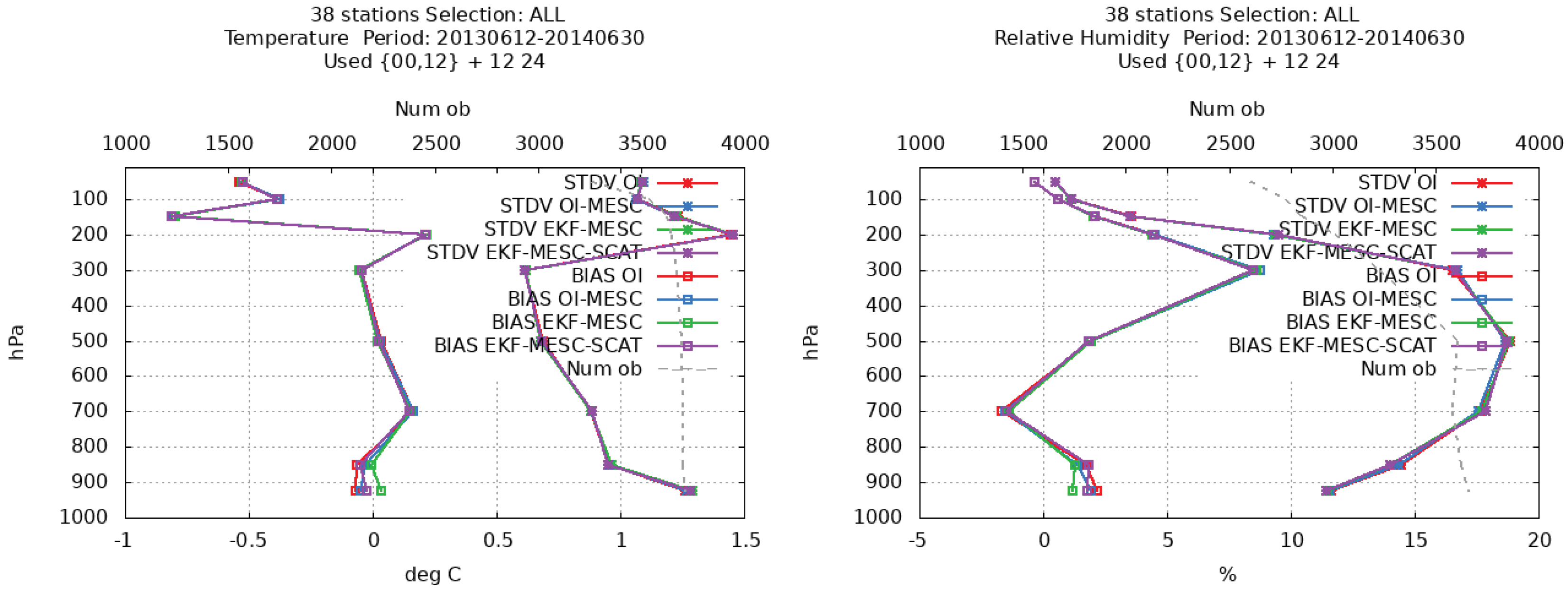
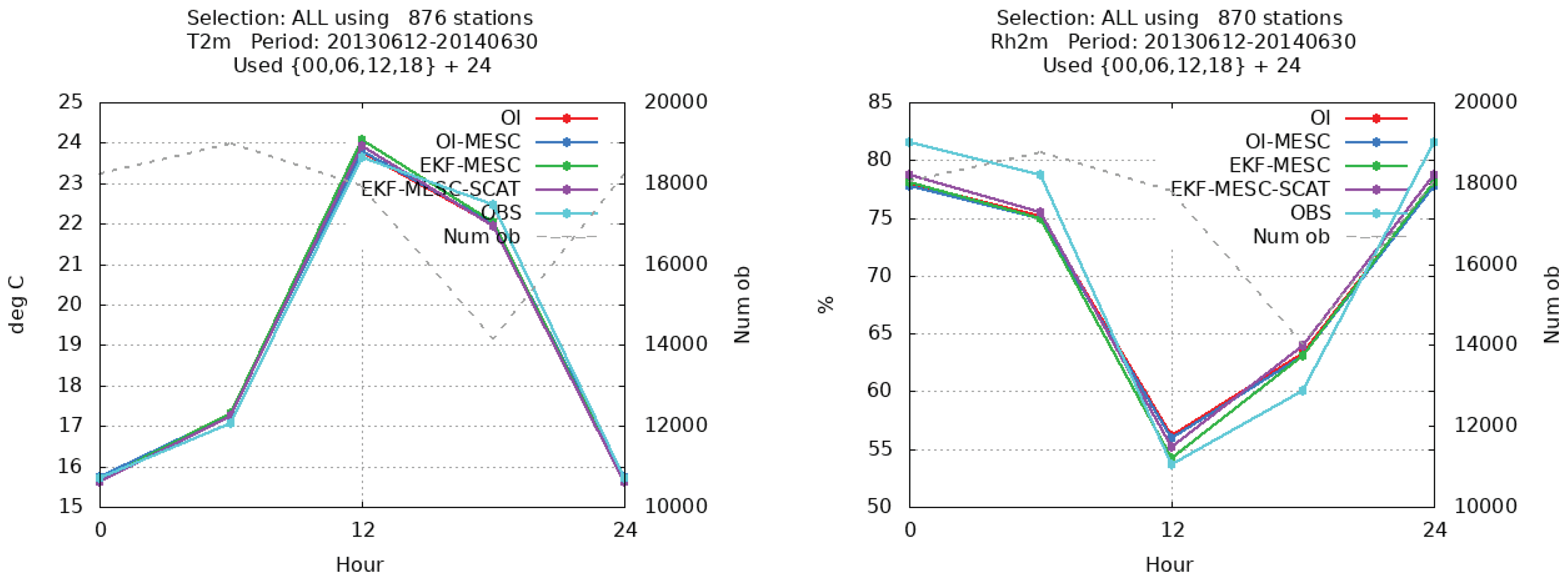
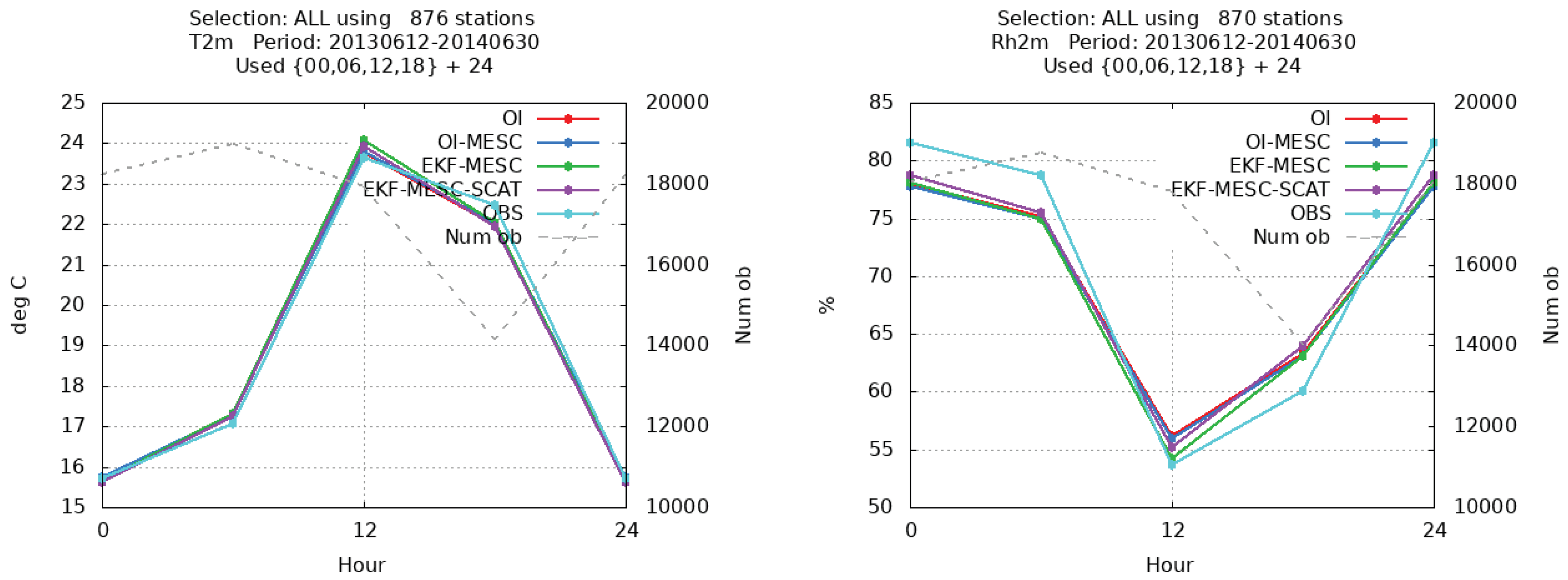
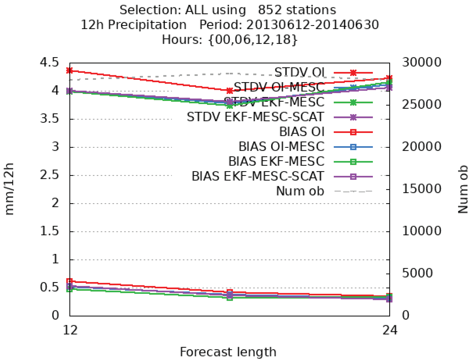
6.1. Objective Verification

One way of measuring forecast quality is to evaluate the model-based weather predictions against available observations. Bias and standard deviation of forecast errors are two typical statistical measures used to quantify systematic forecast errors and the dispersion of the forecast errors. For upper-air variables, the evaluation is typically carried out against radiosonde observations, and for near surface variables, the verification is done against synoptic surface measurements. Synop surface measurements exist over many more locations than radiosonde stations and are also available much more frequently in time, allowing for a larger sample size for the verification.

The objective verification scores for the cases support that the enhanced system has a clear impact. Although the time periods in the experiments are too short to demonstrate statistical significance, we find the impact to be consistent with physics as argued below.

Verification statistics for upper-air the +12-h and +24-h range temperature and humidity predictions are shown in Figure 9. The verification is against radiosonde measurements averaged over all three cases (all within the period from 20130612 to 20140630) presented in Table 1.

Systematic error differences between the different model versions are most evident close to the surface but extend up to mid-troposphere. It seems like the OI-based model version results in larger systematic errors in humidity and temperature predictions as compared to other versions. In terms of dispersion of prediction errors, the impact of methods when obtaining an improved surface-soil moisture state are most clear for humidity and it extends from the surface up to the mid-troposphere.

In Figure 10, scores for two-metre temperature and humidity predictions verified against synop measurements are illustrated. It can be seen that the run with all improvements included (EKF-MESC-SCAT) produced the best forecasts in terms of two-metre relative humidity bias. The improvement of the relative humidity bias (compared to OI) is also consistent with what was seen for low levels when verifying against radiosonde observations in Figure 9. For the runs including only one or two of the methodology enhancements (OI-MESC and EKF-MESC), there is no improvement in terms of two-metre relative humidity bias as compared to the reference system (OI). The scores are rather neutral when it comes to bias and standard deviation of two-metre temperature and standard deviation of two-metre relative humidity. However, the lowest two-metre relative humidity standard deviations are obtained for EKF-MESC-SCAT. The reason for smaller differences between the experiments at zero forecast time as compared with longer ranges is that, at this range, the same observations that have been used in the data assimilation are used also for verification.

Variations between handling of day- and nighttime predictions are illustrated in Figure 11, which illustrates predicted mean values for two-metre temperature and two-metre relative humidity predictions 24 h forward in time as compared with the corresponding observed values. For temperature, the scores are relatively neutral between the experiments and all model versions are in good agreement with synop observations and manage well to capture the daily cycle. On the other hand, forecasts of two-metre relative humidity results in an underestimation of the daily cycle for all model versions. In particular, it seems that nighttime predictions of relative humidity are too low as compared with observations. It can be seen, however, that nighttime two-metre relative humidity forecasts are better for the EKF-MESC-SCAT model version than for the other model versions. In addition, for daytime (12 UTC) conditions, EKF-MESC-SCAT performs slightly better than the reference (OI).

Figure 12 deals with verification scores for predictions of 12 h of accumulated precipitation verified against all synop measurements for a prediction length between +12 and + 24 h. Clearly, the scores depend on the version of parallel experiment, particularly for prediction ranges up to +18 h. Looking at objective verification scores in the form of bias and standard deviation for precipitation, it is clear that all the versions with improved components perform better than the reference version. Based on categorical precipitation scores, like the Kuiper skill score, the improvement is less evident (not shown).

Thus, although the number of cases is too small to derive statistically significant verification scores, the objective results indicate that the enhanced surface data assimilation results in improved short-range NWP precipitation forecasts for severe events. This is consistent with the expectation that a better surface initial state should improve the rainfall forecast.

6.2. Subjective Verification of a Case Study

In the relatively flat land area of the northern continental Europe, a large convective precipitation system developed and moved towards the northeast during the days 26–27 July 2013. The precipitation associated with the system is illustrated in Figure 13, which shows the rain rate in mm per hour as obtained by making use of both information from the satellite-based SEVIRI and SSM/I (Special Sensor Microwave/Imager) instruments based on a multi-sensor approach (https://navigator.eumetsat.int/product/EO:EUM:DAT:MSG:MPE-GRIB).

To illustrate the capabilities of the reference (OI, upper-left) and enhanced (EKF-MESC-SCAT, upper-right) HARMONIE-AROME NWP system to predict the heavy precipitation case, a +36-h forecast launched from 20130726 at 00 UTC of 6 h of accumulated precipitation is presented in Figure 14, together with verifying synop gauge observations (lower right). Comparison of the two figures reveals that the location of the convective system in northern France is better predicted with the enhanced version than with the reference version. While the location of the area with the most intense precipitation is located too far to the west with OI, the location is better predicted with EKF-MESC-SCAT, although still slightly too far to the west. For OI, an EKF-MESC-SCAT overestimates the predicted precipitation amounts as compared to the synop gauge observed amounts. It should furthermore be noted that both model versions predict a precipitation system in southwestern France not supported by observations.

The differences between the two forecasts shown in upper panels of Figure 14 are due to enhancements in deriving the surface initial state and secondary effects due to, for example, the cycling procedure. At one particular time, there were differences not only in surface fields between the forecasts of the different model versions but also in upper-air fields caused by differences in earlier surface initial states and their force on the atmosphere. To illustrate that both the secondary effects from forces on the surface of the atmosphere of previous surface states and the effects from differences in current surface states (also affected by cycling effects) play an important rule, one additional run named EKF-MESC-SCAT OI-UA (UA - Upper-Air) has been carried out for 20130726 at 00 UTC. In this run, upper-air conditions were taken from OI and surface conditions were taken from EKF-MESC-SCAT. The resulting +36-h forecast of 6 h of accumulated precipitation is illustrated in the lower left part of Figure 13. With regard to forecasting the location of the precipitation system in northern France, the EKF-MESC-SCAT OI-UA is somewhat better than the OI-based forecast but worse than EKF-MESC-SCAT, indicating important contributions from both cycling-effect making on upper-air field and of the surface state differences. In Figure 15, it is furthermore demonstrated that such surface state differences between OI and EKF-MESC-SCAT exists. The figure shows differences in the initial state of the $w_2$ soil moisture and the surface temperature for a forecast launched on 20130726 at 00 UTC. The initial state of the EKF-MESC-SCAT version is more moist where the heavy precipitation system develops and propagates. The $w_2$ differences are of the order of 0.03 m³/m³, corresponding roughly to the magnitude of the background error standard deviation derived by Mahfouf [39]. In addition, a surface temperature difference of about 2 K exists between OI and EKF-MESC-SCAT. In general, slightly higher surface temperatures are found for EKF-MESC-SCAT than for OI in the area of activity of the heavy precipitation system in northern France, although some areas with lower temperatures in EKF-MESC-SCAT also exist. Larger $w_2$ soil moisture and top soil level temperatures means enhanced surface to atmosphere heat fluxes creating static instability and conditions favourable for heavy convective precipitation. Interestingly, the location of the area of where EKF-MESC-SCAT generated precipitation in accordance with gauge observations while OI did not coincide with the area where the surface EKF-MESC-SCAT surface initial state is more moist and warmer than the OI surface initial state.

Encouragingly, the refined approach for obtaining an improved surface initial state resulted in a better prediction of the location of the area of heavy convective precipitation. As pointed out by Mahfouf [39], the magnitude of ASCAT data on the the $w_2$ assimilation increments for one particular assimilation cycle is dependent on the Jacobian $\frac{\partial {\mathbf{w}}_g}{\partial {\mathbf{w}}_2}$, of which the magnitude is dependent on the assimilation cycle. Here, we use a rather short assimilation cycle of 3 h, implying smaller but more frequent updates as compared to application of a longer assimilation cycle.

7. Conclusions

This paper presents improved methodologies and enhanced observation usage for data assimilation with a km-scale limited area modelling system. Although one or two of these improvements have been applied before in research and operational systems, they are combined here in a novel system.

Demonstration was made of the performance of the refined NWP system. Three case studies involving strong precipitation events have revealed that the enhancements have an impact on the short-term prediction of precipitation during these events. This is illustrated both by verification statistics and by subjective evaluation of one particular event. It is furthermore shown that the improved procedure for obtaining a surface initial state can lead to a better prediction of severe precipitation events. However, simulations of a much larger number of strong precipitation cases are needed to obtain statistically significant evidence that these enhancements do indeed improve the prediction of heavy precipitation events. Here, the main conclusions are that the surface data assimilation enhancements do have an impact on the prediction of severe precipitation events and that they can improve these forecasts in a way consistent with the expectation that a better surface state improves the rainfall forecasts.

In future work, we will address the difference in scales of representation when comparing values from the model (2.5 km) with the scatterometer product (25 km). Furthermore, issues related to the sharp gradients in the analysis increments occurring close to borders of the satellite swaths need to be addressed. We should furthermore investigate the effect of applying CDF matching methods to relate the ASCAT product to the control variables in the data assimilation, as proposed by Dharssi et al. [38] and by de Rosnay [31]. In addition, extended parallel experiments will be carried out in a preoperational context. These runs should also include various types of quality control, like a background check [40] and rejection in particular areas [39].

References

1. Lorenz, E. A study of the predictability of a 28-variable atmospheric model. Tellus 1965, 17, 321–333. [Google Scholar] [CrossRef] [Green Version]
2. Lindskog, M.; Landelius, T. An Improved System for Short-Term Prediction of Extreme Precipitation Events. IMPREX Deliverable Report 3.2. 2018. Available online: https://www.imprex.eu/system/files/generated/files/resource/deliverable-3-2-imprex-v2-0.pdf (accessed on 25 September 2019).
3. Beljaars, A.; Viterbo, P.; Miller, M.; Betts, A. The anomalous rainfall over the United States during July 1993. Sensitivity to land surface parameterization and soil anomalies. Mon. Weather Rev. 1996, 124, 362–383. [Google Scholar] [CrossRef]
4. Douville, H.; Viterbo, P.; Mahfouf, J.-F.; Beljaars, A. Evaluation of the optimum interpolation and nudging technique for soil moisture analysis using FIFE data. Mon. Weather Rev. 2000, 128, 1733–1756. [Google Scholar] [CrossRef]
5. Drusch, M.; Viterbo, P. Assimilation of screen-level variables in ECMWF’s Integrated Forecast System: A study on the impact on the forecast quality and analyzed soil moisture. Mon. Weather Rev. 2007, 135, 300–314. [Google Scholar] [CrossRef]
6. Mahfouf, J.-F.; Viterbo, P.; Douville, H.; Beljaars, A.; Saarinen, S. A Revised land-surface analysis scheme in the Integrated Forecasting System. ECMWF Newsl. 2000, 88, 8–13. [Google Scholar]
7. Van den Hurk, B.; Ettema, J.; Viterbo, P. Analysis of Soil Moisture Changes in Europe during a Single Growing Season in a New ECMWF Soil Moisture Assimilation System. J. Hydrometeorol. 2008, 9, 116–131. [Google Scholar] [CrossRef]
8. Benjamin, S.G.; Weygandt, S.S.; Brown, J.M.; Hu, M.; Alexander, C.R.; Smirnova, T.G.; Olson, J.B.; James, E.P.; Dowell, D.C.; Grell, G.A.; et al. A North American Hourly Assimilation and Model Forecast Cycle: The Rapid Refresh. Mon. Weather Rev. 2016, 144, 1669–1694. [Google Scholar] [CrossRef]
9. Koster, R.D.; Dirmeyer, P.A.; Guo, Z.; Bonan, G.; Cox, P.; Gordon, C.; Kanae, S.; Kowalczyk, E.; Lawrence, D.; Liu, P.; et al. Regions of Strong Coupling Between Soil Moisture and Precipitation. Sciences 2004, 305, 1138–1140. [Google Scholar] [CrossRef] [Green Version]
10. Koster, R.D.; Mahanama, P.P.; Yamada, T.J.; Balsamo, G.; Berg, A.A.; Boisserie, M.; Dirmeyer, P.A.; Doblas-Reyes, F.J.; Drewitt, G.; Gordon, C.T.; et al. The second phase of the global land-atmosphere coupling experiment: Soil moisture contributions to sub-seasonal forecast skill. J. Hydrometeorol. 2011, 12, 805–822. [Google Scholar] [CrossRef]
11. Weisheimer, A.; Doblas-Reyes, F.J.; Jung, T.; Palmer, T.N. On the predictability of the extreme summer 2003 over Europe. Geophys. Res. Lett. 2011, 38, L05704. [Google Scholar] [CrossRef]
12. Bengtsson, L.; Andrae, U.; Aspelien, T.; Batrak, Y.; Calvo, J.; de Rooy, W.; Gleeson, E.; Hansen-Sass, B.; Homleid, M.; Hortal, M.; et al. The HARMONIE-AROME model configuration in the ALADIN-HIRLAM NWP system. Mon. Weather Rev. 2017, 145, 1919–1935. [Google Scholar] [CrossRef]
13. Mahfouf, J.-F.; Bergaoui, K.; Draper, C.; Bouyssel, F.; Taillefer, F.; Taseva, L. A comparison of two off-line soil analysis schemes for assimilation of screen level observation. J. Geophys. Res. 2009, 114. [Google Scholar] [CrossRef]
14. Muñoz-Sabater, J.; de Rosnay, P.; Albergel, C.; Isaksen, L. Sensitivity of soil moisture analyses to contrasting background and observation error scenarios. Water 2018, 10, 890. [Google Scholar] [CrossRef]
15. Reichle, R.H.; Walker, J.P.; Koster, R.D.; Houser, P.R. Extended versus Ensemble Kalman Filtering for Land Data Assimilation. J. Hydrolmeorol. 2002, 3, 728–740. [Google Scholar] [CrossRef]
16. Schneider, S.; Wang, Y.; Wagner, W.; Mahfouf, J. Impact of ASCAT Soil Moisture Assimilation on Regional Precipitation Forecasts: A Case Study for Austria. Mon. Weather Rev. 2014, 142, 1525–1541. [Google Scholar] [CrossRef]
17. Seity, Y.; Brousseau, P.; Malardel, S.; Hello, G.; Benard, P.; Bouttier, F.; Lac, C.; Masson, V. The AROME-France Convective-Scale Operational Model. Mon. Weather Rev. 2011, 139, 976–991. [Google Scholar] [CrossRef] [Green Version]
18. Cuxart, J.; Bougeault, P.; Redelsperger, J.-L. A turbulent scheme allowing for mesoscale and large-eddy simulations. Q. J. R. Meteorol. Soc. 2000, 126, 1–30. [Google Scholar] [CrossRef]
19. Fouquart, Y.; Bonnel, B. Computation of solar heating of the Earth’s atmosphere: A new parameterization. Beitr. Phys. Atmos. 1980, 53, 35–62. [Google Scholar]
20. Mlawer, E.J.; Taubman, S.J.; Brown, P.D.; Iacono, M.J.; Clough, S.A. Radiative transfer for inhomogeneous atmospheres: RRTM, a validated correlated-k model for the longwave. J. Geophys. Res. 1997, 102, 16663–16682. [Google Scholar] [CrossRef] [Green Version]
21. Masson, V.; Le Moigne, P.; Martin, E.; Faroux, S.; Alias, A.; Alkama, R.; Belamari, S.; Barbu, A.; Boone, A.; Bouyssel, F.; et al. The SURFEX v7.2 land and ocean surface platform for coupled or offline simulations of Earth surface variables and fluxes. Geosci. Model Dev. 2013, 6, 929–960. [Google Scholar] [CrossRef]
22. Noilhan, J.; Planton, S. A Simple Parameterization of Land Surface Processes for Meteo- rological Models. Mon. Weather Rev. 1989, 117, 536–549. [Google Scholar] [CrossRef]
23. Noilhan, J.; Mahfouf, J.-F. The ISBA land surface parameter- ization scheme. Glob. Planet. Chang. 1996, 13, 145–159. [Google Scholar] [CrossRef]
24. Deardorff, J.W. A parameterization of ground surface moisture content for use in atmospheric prediction models. J. Appl. Meteorol. 1977, 16, 1182–1185. [Google Scholar] [CrossRef]
25. Boone, A.; Calvet, J.-C.; Noilhan, J. Inclusion of a third soil layer in a land-surface scheme using the force-restore method. J. Appl. Meteorol. 1999, 38, 1611–1630. [Google Scholar] [CrossRef]
26. Müller, M.; Homleid, M.; Ivarsson, K.-I.; Koltzow, M.; Lindskog, M.; Midtbo, K.-H.; Andrae, U.; Aspelien, T.; Berggren, L.; Bjorge, D.; et al. AROME-MetCoOp: ANordic Convective-Scale Operational Weather Prediction Model. Weather Forecast. 2017, 32, 609–627. [Google Scholar] [CrossRef]
27. Fischer, C.; Montmerle, T.; Berre, L.; Auger, L.; Stefanescu, S. An overview of the variational assimilation in the ALADIN/France numerical weather-prediction system. Q. J. R. Meteorol. Soc. 2005, 131, 3477–3492. [Google Scholar] [CrossRef]
28. Taillefer, F. CANARI—Technical Documentation—Based on ARPEGE Cycle CY25T1 (AL25T1 for ALADIN). 2002. Available online: http://www.umr-cnrm.fr/gmapdoc/ (accessed on 25 September 2019).
29. Giard, D.; Bazile, E. Implementation of a new assimilation scheme for soil and surface variables in a global NWP model. Mon. Weather Rev. 2000, 128, 997–1015. [Google Scholar] [CrossRef]
30. Coiffier, J.; Ernie, Y.; Geleyn, J.-F.; Clochard, J.; Hoffman, J.; Dupont, F. The Operational Hemispheric Model at the French Meteorological Service. In Short and Medium Range Weather Prediction: Collection of Papers Presented at the WMO/IUGG NWP Symposium, Tokyo, 4–6 August 1986; Universal Academy Press: Tokyo, Japan, 1987; pp. 337–345. [Google Scholar]
31. De Rosnay, P.; Drusch, M.; Vasiljevic, D.; Balsamo, G.; Albergel, C.; Isaksen, L. A simplified Extended Kalman Filter for the global operational soil moisture analysis at ECMWF. Q. J. R. Meteorol. Soc. 2013, 139, 1199–1213. [Google Scholar] [CrossRef]
32. Häggmark, L.; Ivarsson, K.-I.; Gollvik, S.; Olofsson, P.-O. Mesan, an operational mesoscale analysis system. Tellus A Dyn. Meteorol. Oceanogr. 2000, 52, 2–20. [Google Scholar] [CrossRef] [Green Version]
33. Soci, C.; Bazile, E. New MESAN-SAFRAN Downscaling System. EURO4M Deliverable D2.5. 2013. Available online: http://www.euro4m.eu/downloads/D2.5_New_MESAN-SAFRAN_downscaling_system.pdf (accessed on 11 September 2019).
34. Soci, C.; Bazile, E.; Besson, F.; Landelius, T.; Mahfouf, J.-F.; Martin, E.; Durand, Y. Report Describing the New System in D2.5. EURO4M Deliverable D2.6. 2013. Available online: http://www.euro4m.eu/downloads/D2.6_Report_describing_the_new_system_in_D2.5.pdf (accessed on 11 September 2019).
35. Draper, C.S.; Mahfouf, J.-F.; Walker, J.P. An EKF assimilation of AMSR-E soil moisture into the ISBA land surface scheme. J. Geophys. Res. 2009, 114, D05108. [Google Scholar] [CrossRef]
36. Wagner, W.; Lemoine, G.; Rott, H. A method for estimating soil moisture from ERS scatterometer and soil data. Remote Sens. Environ. 1999, 70, 191–207. [Google Scholar] [CrossRef]
37. Reichle, R.; Koster, R.; Dong, J.; Berg, A. Global soil moisture from satellite observations, land surface models, and ground data: Implications for data assimilation. J. Hydrometeorol. 2004, 5, 430–442. [Google Scholar] [CrossRef]
38. Dharssi, I.; Bovis, K.J.; Macpherson, B.; Jones, C. Operational assimilation of ASCAT surface soil wetness at the Met Office. Hydrol. Earth Syst. Sci. 2011, 15, 2729–2746. [Google Scholar] [CrossRef] [Green Version]
39. Mahfouf, J.-F. Assimilation of satellite-derived soil moisture from ASCAT in a limited-area NWP model. Q. J. R. Meteorol. Soc. 2010, 136, 784–798. [Google Scholar] [CrossRef]
40. Lindskog, M.; Ridal, M.; Thorsteinsson, S.; Ning, T. Data assimilation of GNSS zenith total delays from a Nordic processing centre. Atmos. Chem. Phys. 2017, 17, 13983–13998. [Google Scholar] [CrossRef] [Green Version]
Figure 1. Model area (red rectangle) and event evaluation area (blue circle).
Atmosphere 10 00587 g001
Figure 2. SEVIRI instrument infrared brightness temperature on 20130727 at 03.30 UTC (unit: K).
Atmosphere 10 00587 g002
Figure 3. Demonstration for 20130614 at 09 UTC of the procedure for conversion of scatterometer product (unit: %) to w g a s c a t , uppermost model level soil moisture (unit: m3/m3).
Atmosphere 10 00587 g003
Figure 4. Illustration of the collocation methodology of scatterometer soil moisture product from MetOp-A (green) and MetOp-B (red) for 20140614 at 09 UTC: The resulting data to be used within the surface-soil data assimilation are marked blue.
Atmosphere 10 00587 g004
Figure 5. Model versions used in the parallel experiments and illustration of adding components through successive enhancements of the reference system (OI).
Atmosphere 10 00587 g005
Figure 6. Effect of screen-level temperature of a single temperature observation located in the valley in the Alps and 1.5 K larger than the background equivalent (unit: K) using reference background error statistics (left) and MESCAN (middle): Also shown is model orography in meters (right).
Atmosphere 10 00587 g006
Figure 7. Statistics based on a ten-day period (20140621 to 2013062830) of Jacobian values for surface grid-points for T 2 m T 2 (left, unit: 1/m3/m3) and RH 2 m w 2 (right, unit: K/K): Statistics are both for daytime (blue histograms) and nighttime (red histograms) conditions.
Atmosphere 10 00587 g007
Figure 8. Data assimilation increments of soil moisture in the top and second soil layers are shown in the upper and lower panels, respectively. Results for the OI experiment are depicted to the left, and the ones for the EKF-MESC-SCAT experiments are to the right. All maps refer to the date 20140625 at 18 UTC, and the unit is % of change of the corresponding background value.
Atmosphere 10 00587 g008
Figure 9. Verification statistics in terms of bias and standard deviation of predictions against radiosonde observations of temperature (left, unit: K) and relative humidity (right, unit: %) averaged over the three cases: Scores are accumulated over +12-h and +24-h prediction ranges and shown as a function of the vertical level. Different colours are for different model versions within the parallel experiment. The grey dashed curve illustrates the number of observations used within the verification.
Atmosphere 10 00587 g009
Figure 10. Verification statistics in terms of bias and standard deviation of predictions against synop observations of two-metre temperature (left, unit: K) and two-metre relative humidity (right, unit: %) averaged over the three cases: Scores are shown as a function of prediction length in hours, and different colours are for different model versions within the parallel experiment. The grey dashed curve illustrates the number of observations used within the verification.
Atmosphere 10 00587 g010
Figure 11. Mean +24-h forecast of two-metre temperature (left, unit: K) and two-metre relative humidity (right, unit: %) as compared with synop observations as a function of time within the day: Different colours are for different model versions within the parallel experiment and for observations. Scores are averaged over the three cases. The grey dashed curve illustrates the number of observations used within the verification.
Atmosphere 10 00587 g011
Figure 12. Verification scores in terms of bias and standard deviation of predictions against synop observations of 12 h of accumulated precipitation (unit: mm/12 h) and averaged over the three cases: Scores are shown as a function of prediction length in hours, and different colours are for different model versions within the parallel experiment. The grey dashed curve illustrates the number of observations used within the verification.
Atmosphere 10 00587 g012
Figure 13. Rain rate (mm/h) for a convective heavy precipitation event on 20130727 at 19.00 UTC (upper left), on 20130728 at 03.15 UTC (upper right), and on 20130728 at 08.30 UTC (lower left): The estimates are based on a multi-sensor approach.
Atmosphere 10 00587 g013
Figure 14. Predictions at +24 h of 6 h of accumulated precipitation (unit:mm/6 h) valid between 20130727 at 00 UTC and 20130727 at 06 UTC with OI (upper left), EKF-MESC-SCAT (upper right), and EKF-MESC-SCAT OI-UA (lower left): Also shown are the corresponding 6-h accumulated rain gauge observations (lower right).
Atmosphere 10 00587 g014
Figure 15. EKF-MESC-SCAT and OI w 2 soil moisture (unit: m3/m3) and and top soil level temperature (right: unit: K) differences for the analysis valid on 20130726 at 06 UTC.
Atmosphere 10 00587 g015