Analysis of a Sea Fog Episode at King George Island, Antarctica

Abstract

In this study, a marine fog episode at King George Island off the Antarctic Peninsula from 26–30 January 2017 was investigated using surface observations, upper-air soundings, and re-analysis data as well as the air mass backward trajectory method. The marine fog episode resulted from an approaching low-pressure system, was maintained at high wind speeds, and quickly dissipated when the low-pressure system passed the observation site. During this episode, cloud lay existed above the fog and stratus, the atmosphere was stably stratified for 1600 m, and the air close to the surface was more mixed than air in the upper layer. The air-sea temperature difference (ASTD) of 1–2 °C and a strong surface wind parallel to the gradient of SST were two important factors in the formation and maintenance of the marine fog near the Antarctic region. The convergence of flux for both water vapor and heat during the fog episode was also discussed.

1. Introduction

Marine fog [1] reduces visibility to less than 1 km and is responsible for 32% of worldwide sea accidents [2]. Regarding global warming [3], changes in marine fog occurrence correspond well with horizontal temperature advection changes near the surface in numerical simulations, including the Southern Ocean around Antarctica [4]. Fog and mist over polar seas are highest in the summer and are rarely observed during winter [5], and the process of their onset, maintenance, and disappearance are all closely related to interactions between the atmosphere, sea, land, and ice.

The cold sea fog investigated by Taylor [6] represents the first major study on sea fog [1]. Lewis et al. [7] contrasted synoptic conditions for fog and fog-free events, and they found that the strength and evolution of synoptic-scale subsidence, the strength and height of marine inversion, the air-sea temperature difference, cloudiness at the top of the marine layer, and air mass transformation along trajectories were causes of sea fog formation. However, the importance of these factors differs in sea fog cases. For example, cold sea fog along the U.S. western coast usually occurs from warm offshore airflow erosion, and the marine inversion almost reaches the sea surface [8,9] where long-wave radiation helps in cooling and in rapid fog growth [10,11,12]. Along the eastern coast of Scotland, the fogged air initially cools from contact with the cold sea, followed by radiative cooling and lowering of the fog temperature below the surface temperature; this initiates convective and radiative heat input from the sea surface and entrainment of warm air at the top of the fog [13]. Cold sea fog at the Yellow Sea usually involves a prominent inversion at 100 m to 350 m altitude [14], and the inverted and dry layer generated by subsidence plays a major role in the formation of the sea fog [15]. Gradual cooling and moistening by turbulent mixing also produce sea fog [16].

Compared with the Antarctic, more research is available on Arctic fog, as exemplified by the publication “The Climate of Arctic” [17]. Fog is abundant during the ice melting season in the Arctic, with sea fog being the most common type [18,19,20]. Temperature inversions occur in over 80% of Arctic summer soundings [21,22] and promote the formation and maintenance of fog [23,24,25]. High Arctic fog frequently resides in an elevated inversion layer, whereas low Arctic fog is often restricted to the mixed layer [26]. King George Island is in the South Shetland Islands at the edge of the Antarctic Peninsula. It is among the most densely populated parts of Antarctica and is visited by an increasing number of tourists annually [27]. The probability of fog increases in the area as northerly winds usher a warm air front, producing fog even in the presence of strong winds [27]. Fog occurs, on average, 73 days annually [28], with most of it being considered cold sea fog (also named as cold fog, warm advection fog, and advection cooling fog [1,29]). It is attributed to condensation of northwesterly warm air advection from the South Pacific Ocean while flowing over the cold circumpolar sea [28].

The complicated evolution of a marine fog indicates that a forecaster’s experience is valuable in accurate fog forecasting [1,30]. In a harsh environment like the Antarctic region, few observation experiments on fog have been undertaken. Matthew et al. observed fog particles around McMurdo Station, Antarctica, showing that the fog droplets appeared to be approximately 7.5 to as much as 10 microns in size [31]. Khwairakpam et al. investigated an episode of coastal advection fog over East Antarctica oases recorded by monostatic acoustic sodar, and they showed that this type of fog was an important source of water for microbes [32]. Overall, marine fog processes in the Antarctic region are largely unknown [4,5]. The aim of this paper is to elucidate the development of King George Island marine fog through site observations and to highlight the dominant processes of its formation in the area.

2. Data and Methodology

Field observation data in this study were obtained from the Chinese Antarctic science research site. The site hosts the Great Wall Station (World Metrological Organization identifier 89058) on King George Island (Figure 1) at an elevation of 10 m above sea level. High-quality, conventional meteorological parameters, including wind speed, wind direction, humidity, and pressure on the ground per hour, were recorded.

A forward scatterometer, PWD-20 (Vaisala) was used to monitor visibility. Its effective measurement range is from 0 to 20 km, with a bias of 10% and 15% for 0–10 and 10–20 km distances, respectively. Observations using PWD-20 can be affected by large buildings and other objects that generate heat or impede precipitation. To avoid this, the equipment was set on a hill 300 m away from the Great Wall Station at an elevation of about 29 m. The visibility was recorded every minute, and we calculated its hourly means after removing peaks in data series that might be caused by worms, dew, and so on. Details about the equipment and quality control method can be found in the article by Yang et al. [33].

Radiosondes (RS-92, Vaisala) were launched once a day at the Great Wall Station around 1200 (UTC, the same hereafter, corresponding to 0900 LST) from 10 January to 10 February 2017. This study mainly focused on the period from 25–30 in January. The air pressure, temperature, relative humidity, wind direction, and wind speed were measured every 2 s with a vertical resolution of 4–10 m. Similar radiosondes have been used in studying fog episodes off the coast of southern China [34,35].

The entire ground observation lasted for one month. Several fog episodes were recorded, but most of them vanished quickly and lasted only for a few hours. We picked a fog case that existed from 27–29 January in this study, and we tried to analyze the contribution of large-scale circulation on this fog process.

Real-time global sea surface temperature analysis data (http://polar.ncep.noaa.gov/sst/) with a resolution of 0.083° and 0.5° were selected from the National Centers for Environmental Prediction (NCEP) [36]. We obtained backward airflow trajectories using the HYSPLIT trajectory online model [37,38], with the Global Data Assimilation System set as the basic data (http://www.emc.ncep.noaa.gov/gmb/gdas/). We downloaded NCEP FNL (final) operational model global tropospheric analyses data with a resolution of one-degree from the NCEP/National Weather Service (NWS)/NOAA/U.S. Department of Commerce [39]. The sea surface flux, including latent and sensible heat fluxes, was provided by NCEP [40].

To diagnose atmospheric physical processes, the heating rate resulting from the convergence of the heat flux is written as:

$$T_{con}=-\nabla ·\left(\overrightarrow{V}T\right),$$

(1)

and the condensation (precipitation) resulting from the convergence of the moisture flux is:

$$q_{con}=-\nabla ·\left(\rho \overrightarrow{V}q\right).$$

(2)

In Equations (1) and (2), $\nabla$ stands for the calculation of divergence in three directions, $\overrightarrow{V}$ is the 3-D wind vector (u, v, ω), $T$ is the air temperature, $q$ is the atmospheric specific humidity, and $\rho$ is the air density. The heating or condensation controlled by large-scale circulation was not the only factor controlling the thermal dynamics process within the atmosphere, for example, atmospheric turbulence-induced transport might also be important in the atmospheric boundary layer, but they are indeed important terms in balance equations for energy and (water) mass within the atmosphere.

3. Results and Discussion

3.1. Surface Meteorological Conditions

Figure 2 shows the temporal variations of visibility, precipitation, relative humidity, temperature, wind speed, and wind barb recorded at Great Wall Station. A marine fog episode occurred near King George Island in the summer between 25–30 January 2017. Light precipitation prior to and during the two sea fog periods suggests it promotes formation and maintenance of fog [41]. Visibility started declining on January 26 and approached 1 km at 08:00, 09:00, and 15:00. Sea fog appeared at 0000 UTC on 27 January and lasted for 14 h (Figure 2a). The visibility improved to over 1 km from 1400 UTC on 27 January to 1500 UTC on 28 January (Figure 2a). Another sea fog episode emerged at 1600 UTC on 28 January and lasted through 29 January, with visibility below 1 km for 32 h. The visibility improved again on 30 January, marking the end of the second sea fog episode.

The relative humidity during the two sea fog periods was ≥96% (Figure 2b), which coincided with the maximum relative humidity on the ground, and exceeded that during precipitation. The surface air temperature varied from 2.8 °C to 3.9 °C during the two sea fog episodes (Figure 2c). The sea fog disappeared at surface temperatures >4 °C or <3 °C. Considering that the sea temperature is relatively stable, when the air temperature changes significantly, the sea–air interaction changes, which may be detrimental to the formation and maintenance of sea fog. The sea fog suspended and ended, while the prevailing wind direction changed from NNW to WNW late on 27 January and early on 30 January. It is conceivable that compared to the west wind, northerly wind means warmer and moister air, which is very important for the maintenance of sea fog. The fog formed after several hours of a pressure drop early on 27 January and late on 28 January, indicating that the fog episode was caused by a low-pressure system.

The wind speed exceeded 6 m·s⁻¹ during the fog episode, and the fog was maintained even at wind speeds above 10 m·s⁻¹ (Figure 2d), typical of a windy sea fog process [27,28]. Filonczuk et al. [42] analyzed multiyear data from a set of coastal weather stations (such as San Diego and San Francisco) and comprehensive marine weather reports (primarily ships) along the California coast. The analysis revealed fog was associated with all wind classes, but most sea fog occurred at wind speeds below 4–6 m·s⁻¹, although it was present in northern regions at speeds near 15 m·s⁻¹ in winter months. Song [43] and Wang [44] analyzed multiyear International Comprehensive Ocean-Atmosphere Data Sets and reported sea fog occurs over the northern Pacific and the northern Atlantic primarily at wind speeds from 4.4 to 12.3 m·s⁻¹. Therefore, although the wind speed of the marine fog episode in this study was high, it was not destructive.

3.2. Synoptic Background

The synoptic background for the fog episode during 25–30 January is depicted in Figure 3. It can be seen that a strong low-pressure system moved from the eastern South Pacific to the Bellingshausen Sea during 25–30 January (Figure 3a–e), crossed the Antarctic Peninsula, and went into the Weddell Sea afterward on 30 January (Figure 3f). Thus, the formation and maintenance of the fog episode seemed to be linked with the passing of the low-pressure system. Previous studies on sea fog pointed out that sea fogs intend to occur with a high-pressure system because a continuous subsidence circulation might lower the stratus to form fog [7,9,14]. In contrast, the increase in air pressure on 28 January (Figure 2b) corresponded to a period of pause for the fog episode (Figure 3d). Thus, we suggested that subsidence due to the ridge might not be essential in the formation of this episode.

Throughout the fog episode, it should be noted that the surface wind direction and SST gradient was quite steady (Figure 3). The SST reduced gradually from 7 to 1 °C, from the north to south across the Drake Passage, and maintained such distribution during the fog episode. The northwesterly winds modulated by the synoptic system were perpendicular to SST isotherms over the Drake Passage at the upper side of the Great Wall Station from 26–29 January (Figure 3b–e). On 30 January, when the surface wind was parallel to the SST isotherms, the fog episode ended. Therefore, when the surface wind was strong and on the same direction as the SST gradient, the warm and humid air was continuously transported to a region with a cold sea surface, which might have triggered the sea fog as observed in this study. Such a mechanism was also recognized in several pieces of literature [1,6,29]. It should be noted that when the fog began to suspend at 1300 on January 27, the wind direction also changed from northerly to westerly. So, we suggested that whether the surface wind was in the same direction as the SST gradient was a crucial factor in forming the sea fog episode.

3.3. Boundary Layer Structure

To investigate the boundary layer structure during the fog episode, humidity, temperature, and virtual potential temperature were analyzed and are displayed in Figure 4. Sounding occurred even after fog onset on 26 January. Since the surface sea fog dissipated to mist at average relative humidity <98% during the observation period, Huang et al. [34,35] considered a relative humidity of 98% as the top (or base) of the sea fog and clouds. In this study, surface visibility was <1 km when the relative humidity was ≥96%. Thus, we defined the relative humidity of 96% as the top (or base) of the sea fog and clouds. However, it should be noted that the reliability of a radiosonde and scatterometer used in extremely humid conditions (like fog in this study) should be questioned; thus, the critical value of relative humidity given here (such as 96%) was just a reference rather than a convincing conclusion.

In some other advection fog cases, the sky was free above the stratus, and long-wave radiation out from the stratus top could cool the stratus and eventually lower the stratus to fog [8,9,11,12]. We suggest that in the case studied, the cloud layer over fog or the stratus prevented solar radiation from warming the fog in the daytime and inhibited the cooling due to long-wave radiation at the top of the fog. On 25 and 30 January, the cloud cover in the upper atmosphere below 1600 m altitude was low (Figure 4a,f). A cloud layer over the fog and stratus existed from 26–29 January (Figure 4b–e). This occurrence is consistent with the common observation of multiple cloud layers separated by uncoupled subcloud layers in polar areas [45,46,47].

The height of the stratus top on 28 January was lower than that of the fog top on 27 and 29 January. The relative humidity curve on 28 January further indicated that a significant entrainment layer existed between 1200 and 1600 m (Figure 4d), which might be caused by subsidence due to the high-pressure ridge. Besides, the change in surface wind direction on 28 January, which might have reduced the water vapor fluxes, should be more critical in the suspension of the fog episode (Figure 2e).

Low-level elevated inversion (compared to surface-based inversion) occurred from 26–30 January, with a strength less than 2.0 °C and height below the top of the fog (Figure 4b–f). The temperature of the top of the fog (stratus) hovered close to 1.5 °C from 27–29 January, being close to the SST near King George Island. The temperature difference between air and sea surface remained close to 1.5 °C during the fog episode. Gao et al. [16] employed the Mesoscale Model 5 [48] to analyze a cold sea fog event over the Yellow Sea. Their study showed that sea fog formed in response to gradual cooling and moistening by turbulent mixing in the region between the inversion base and the sea surface. This region is considered a well-mixed layer. In this study, although the layer under 100 m seemed to be well-mixed by wind-induced turbulence, stratification within the whole fog layer was stable, which was seen from the profile of virtual potential temperature.

In some cases, fog forms as a stratus-lowering process and, thus, can be considered as a cloud in contact with the sea surface [11]. In other cases, the fog forms immediately above the sea surface and then expands vertically to form a cloud [13]. By viewing the low-level cloud observed before fog onset on 25 January and the stratus on 28 January, the fog episode may be considered as a stratus-lowering process.

3.4. Dynamic Process Analysis

3.4.1. Backward Trajectory Analysis

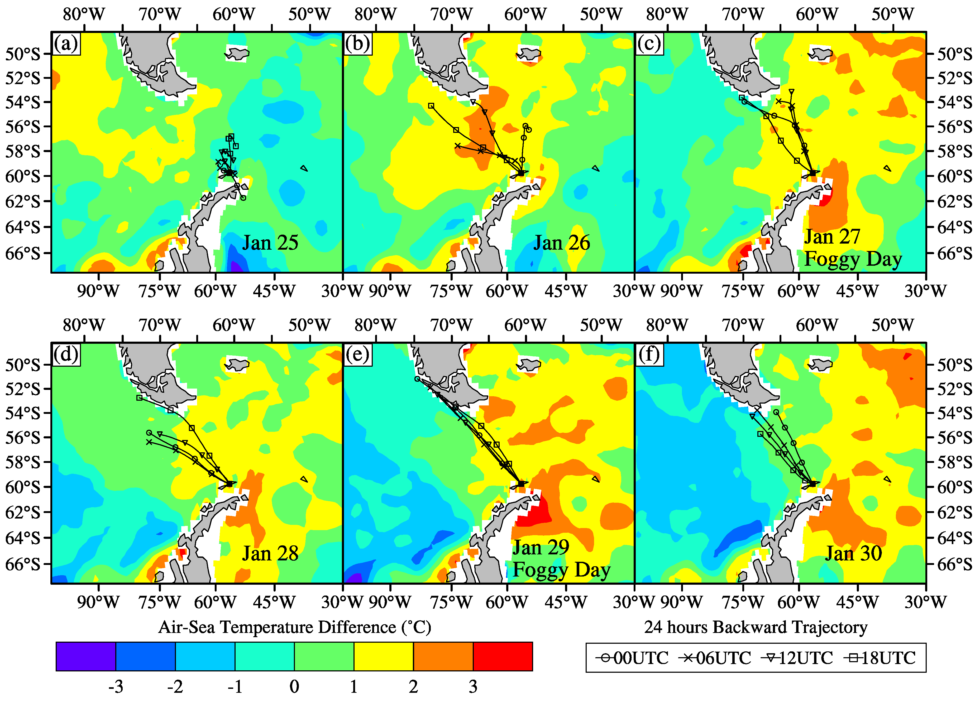
The key factor in a sea fog episode is the saturation level of the near-surface air. The trajectory analysis of an air mass, introduced by Taylor [6], is a widely utilized and effective method to diagnose the cooling and moistening during advection [7,11,12,49,50,51]. According to Heo and Ha [52], most advection fog occurs when the air temperature is approximately 1–2 °C warmer than the SST. Wang [29] emphasized that, in the case of cold sea fog, the proper air-sea temperature difference (ASTD, hereafter) for moistening and cooling the capping air is 0–2 °C. Generally, the closer the ASTD is to 2 °C, the higher the frequency of fog.

We initially applied a 24 h back trajectory analysis four times daily using the HYSPLIT trajectory model available on the website of NOAA Air Resources Laboratory (http://www.arl.noaa.gov). The Great Wall Station represented the end point, while the height concerned was at 10 m above sea level. The difference between the air temperature at 2 m in FNL and the SST yielded the ASTD.

The back trajectory analysis demonstrated the upper stream air of the sea fog originated from regions with ASTD > 0 °C, characteristic of a cold sea fog episode. The ASTD for back trajectories increased from less than −1 °C to more than 2 °C from 25 to 26 January, and it was maintained at >1 °C until 30 January. In addition, the back trajectories began to concentrate when the low-pressure system approached, especially on 29 and 30 January (Figure 5). However, since the ASTD for the trajectories was <1 °C on 30 January, the fog episode ended. Therefore, from the back trajectory analysis, it seemed that a greater ASTD was more important than a steady surface wind for the maintenance of sea fog. But, it should be noted that when the ASTD was much larger, air capping on the sea surface will become more difficult to be saturated [29], which might prevent the forming of fog. Therefore, the ASTD of 1–2 °C might be most beneficial for sea fog formation.

3.4.2. Validation of Analysis Data

The limited information derived from observations induces a resort to analysis data. The reliability of the analysis chosen initially necessitates an evaluation. The temperature and relative humidity from radiosonde observations were consistent with the analysis dataset FNL (Figure 6), with an average absolute bias of 1.97 °C and 7.60%, respectively. The near-surface values of relative humidity reached highs on 26, 27, and 29 January and decreased to a low value early on 28 January. Therefore, although the relative humidity data differ slightly from in situ observations, the analysis data enables investigation of the marine fog episode near King George Island, Antarctica.

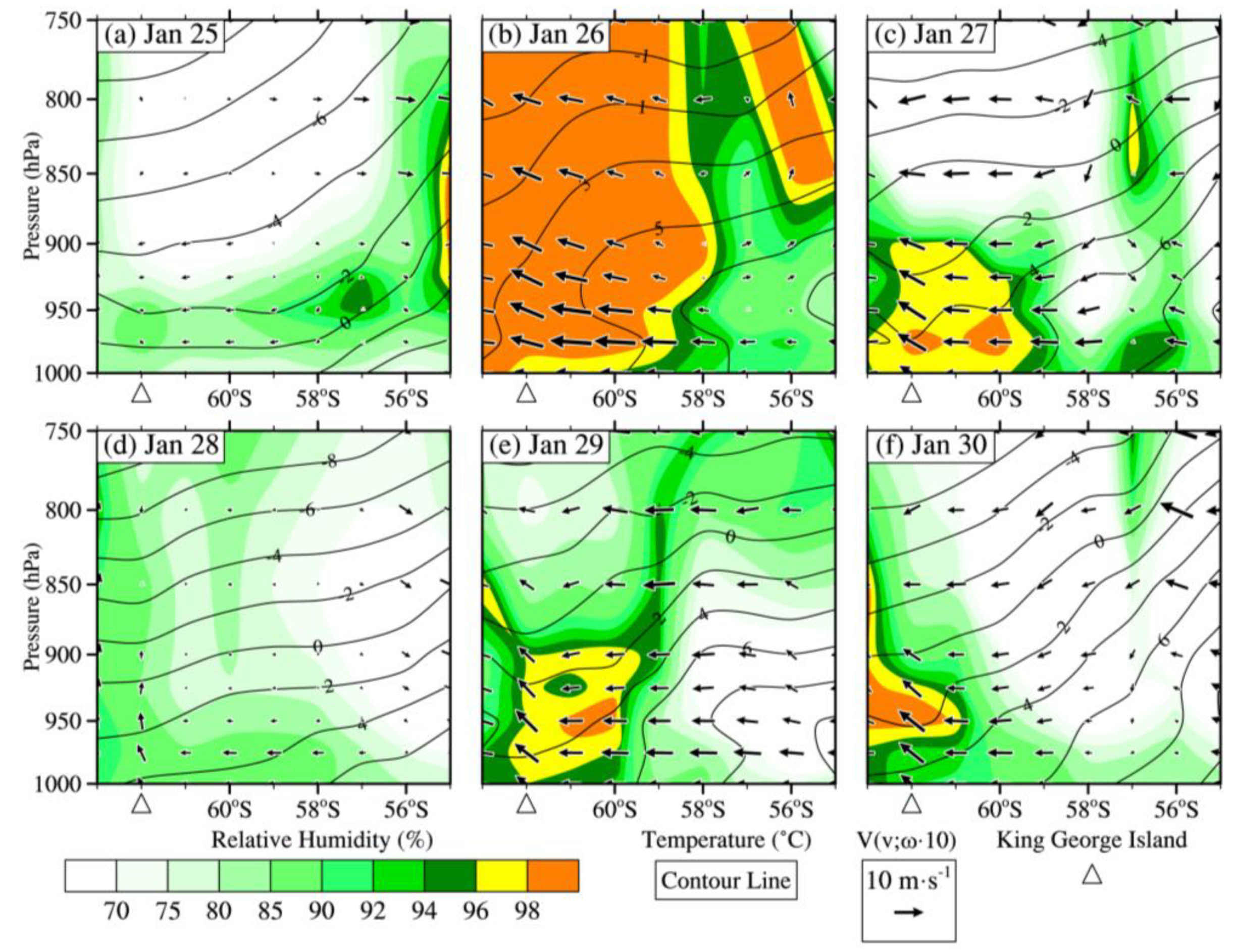
Figure 7 illustrates the vertical section of the thermal structure of the atmosphere over the Drake Passage across King George Island (the surface scope is shown in Figure 1 as the red dotted line) at 0600 UTC from 25–30 January. It showed that the relative humidity of air below 900 hPa was relatively low, and the wind speed in the north component was weak on 25 and 28 January. Conversely, the relative humidity was relatively high, and the wind speed in the north component was strong on 26, 27, 29, and 30 January. Temperature inversion occurred north of King George Island near 59° S, accompanied by a decrease in strength from 26–27 and 29 January. This indicated that the increase in relative humidity primarily resulted from warm advection from the north.

4 Discussion

As in the analysis above, the FNL data can approximately capture the structure of the atmosphere for this fog episode; thus, the effect of large-scale circulation from it might also be representative. The large-scale circulation might be important for this episode, so the convergence of heat (T_con) and the convergence of water vapor flux (q_con) were calculated using Equations (1) and (2) (Figure 8). It should be noted that the vertical integration of q_con has the same unit as surface evaporation/precipitation.

The variations of q_con and T_con were similar from 25–30 January: a positive center for T_con and q_con located between 975 and 850 hPa, and a weak but divergent one was underneath it (Figure 8a). On 26 January, much stronger, but negative, q_con and T_con appeared near the surface, which corresponded to a period of rain. When the negative q_con and T_con near-surface values became moderate, like on the dawn of 27 January and the afternoon on 28 January, the fog began. When there was no negative q_con and T_con near the surface, like on 30 January, and even though there was still strong, positive q_con and T_con values near the 950 hPa level, the fog stopped. The distribution of q_con and T_con means that the advection of large-scale circulation caused heating in the layer of 950–700 hPa and cooling beneath it. The heating and cooling will help to keep a stable stratification in the lower troposphere, which might be a benefit for sustaining the fog. It should be noted that heating due to T_con and q_con was quite large; thus, it can change the stratification of the lower atmosphere quickly. But, the observed profiles of atmosphere during the foggy period were quite stable (Figure 4, Figure 6), and there must have been another kind of process that balanced the heating.

The downward latent and sensible heat flux near the sea surface appeared during most of the period from 25–30 January, and reached their maxima on 26 January and late on 28 January (Figure 8b). The turbulence within the boundary layer delivered both heat and water vapor from the atmosphere into the sea, damping the condensation, and was accompanied by heating in the layer of 950–700 hPa. Because the turbulent fluxes were significant when the surface wind speed was greater than 5 m·s⁻¹, it seems that a strong wind might be critical for the fog near the Antarctic region not only because it continuously induced advection of warm and humid air from north, but also because it maintained the local turbulent intensity within the atmospheric boundary layer.

The warm advection and sea surface cooling promoted sea fog, consistent with previous studies [3,52,53,54]. Heo et al. [53] analyzed in situ observations over the Yellow Sea and showed latent heat flux changes up to −200 to −100 W·m⁻² and sensible heat flux changes up to −70 W·m⁻² during the maturity of advection sea fog. Heo and Ha [52] showed that advection fog is obviously controlled by low-level atmospheric stability and downward latent heat flux with oceanic cooling. Huang et al. [54] improved the regional prediction of sea fog along the Guangdong coastland by using the temperature difference of 1000 hPa and 2 m.

The downward sensible heat flux was stronger than the latent heat flux in this study. This is opposed to cases reported in the Yellow Sea, where latent heat flux dominates [52,53]. The difference might be caused by the fact that the Bowen ratio of seawater depended on SST. However, a turbulent flux was obtained from FNL, and the real surface turbulent heat flux during the fog episode is still unknown.

5. Summary and Conclusions

A marine fog episode near the Great Wall Station at King George Island, Antarctica, was closely monitored, and its vertical structure was recorded by radio sounding. The large-scale circulation during the episode was investigated using analysis data and the air mass backward trajectory model. The onset of the fog was early on 27 January 2017, followed by suspension late on 27 January, a reappearance late on 28 January that lasted through 29 January, and disappearance early on 30 January 2017. The main findings are summarized as follows:

(1) The sea fog episode started as a low-pressure system approached, was suspended when a high-pressure ridge invaded the area, and ended after the low-pressure system passed. Site observations that reveal the surface meteorological conditions suitable for the formation and sustenance of fog included a warm and humid surface air as well as a relatively steady wind direction. Fog tended to dissipate or was suspended when the prevailing wind direction changed from northerly to westerly.

(2) The warm and humid air was advected by northwesterly winds induced by the low-pressure system. The advected air was cooled and moistened near the sea of the Drake Passage in the southern Pacific Ocean. Because of the warm advection process, the air was warmer than the sea surface and caused a stable stratification within the fog layer. The optimum temperature difference between air and sea for the fog near the Antarctic region might vary between 1–2 °C.

(3) In the initial stage of the fog, there were significant convergences for heat and water vapor fluxes in the layer from 950 to 700 hPa, and weak divergences appeared underneath this layer. Meanwhile, the surface latent and sensible heat fluxes were both downward. The downward sensible and latent heat fluxes can offset the heating effect due to the convergent large-scale circulation, which might be a benefit for the maintenance of sea fog.

References

- Koračin, D.; Dorman, C.E.; Lewis, J.M.; Hudson, J.; Wilcox, E.; Torregrosa, A. Marine fog: A review. Atmos. Res. 2014, 143, 142–175. [Google Scholar]
- Tremant, M. La Prévision du Brouillard en. In Mer. Météorologie Maritime et Activities Océanographique Connexes (Rapport No. 20. TD no. 211); World Meteorological Organization: Geneva, Switzerland, 1987. [Google Scholar]
- IPCC. Climate Change 2013: The Physical Science Basis. Contribution of Working Group I to the Fifth Assessment Report of the Intergovernmental Panel on Climate Change; Cambridge University Press: Cambridge, UK; New York, NY, USA, 2013; p. 1535. [Google Scholar]
- Kawai, H.; Koshiro, T.; Endo, H.; Arakawa, O.; Hagihara, Y. Changes in marine fog in a warmer climate. Atmos. Sci. Lett. 2016, 17, 548–555. [Google Scholar] [CrossRef] [Green Version]
- Dorman, C.E.; Mejia, J.; McEvoy, D.; Koračin, D. Worldwide Marine Fog Occurrence and Climatology. In Marine Fog: Challenges and Advancements in Observations, Modeling, and Forecasting; Koračin, D., Dorman, C.E., Eds.; Springer: Cham, Switzerland, 2017; pp. 7–152. [Google Scholar]
- Taylor, G.I. The Formation of Fog and Mist. Q. J. R. Meteorol. Soc. 1917, 43, 241–268. [Google Scholar] [CrossRef]
- Rabin, R.; Businger, J.; Lewis, J.; Koracin, D. Sea fog off the California coast: Viewed in the context of transient weather systems. J. Geophys. Res. Space Phys. 2003, 108, 1–17. [Google Scholar]
- Leipper, D.F. Fog development at San Diego, California. J. Mar. Res. 1948, 7, 337–346. [Google Scholar]
- Leipper, D.F. Fog on the U.S. west coast: A review. Bull. Am. Meteorol. Soc. 1994, 75, 229–348. [Google Scholar] [CrossRef]
- Pilie, R.J.; Mack, E.J.; Rogers, C.W.; Katz, U.; Kocmond, W.C. The Formation of Marine Fog and the Development of Fog-Stratus Systems along the California Coast. J. Appl. Meteorol. 1979, 18, 1275–1286. [Google Scholar] [CrossRef] [Green Version]
- Koračin, D.; Lewis, J.; Thompson, W.T.; Dorman, C.E.; Businger, J.A. Transition of Stratus into Fog along the California Coast: Observations and Modeling. J. Atmos. Sci. 2001, 58, 1714–1731. [Google Scholar] [CrossRef]
- Koračin, D.; Businger, J.A.; Dorman, C.E.; Lewis, J.M. Formation, Evolution, and Dissipation of Coastal Sea Fog. Bound. Layer Meteorol. 2005, 117, 447–478. [Google Scholar]
- Findlater, J.; Roach, W.T.; McHugh, B.C. The haar of north-east Scotland. Q. J. R. Meteorol. Soc. 1989, 115, 581–608. [Google Scholar] [CrossRef]
- Zhang, S.P.; Xie, S.P.; Liu, Q.Y.; Yang, Y.Q.; Wang, X.G.; Ren, Z.P. Seasonal Variations of Yellow Sea Fog: Observations and Mechanisms. J. Clim. 2009, 22, 6758–6772. [Google Scholar] [CrossRef]
- Zhang, S.P.; Liu, F.; Kong, Y. Remote relationship in origination of sea fog in East China Sea to the stratus in Yellow Sea in spring. Oceanol. Limnol. Sin. 2014, 45, 341–352. (In Chinese) [Google Scholar]
- Gao, S.; Lin, H.; Shen, B.; Fu, G. A heavy sea fog event over the Yellow Sea in March 2005: Analysis and numerical modeling. Adv. Atmos. Sci. 2007, 24, 65–81. [Google Scholar] [CrossRef]
- Przybylak, R. The Climate of the Arctic; Springer International Publishing: Cham, Switzerland, 2016; p. 287. [Google Scholar]
- Nilsson, E.D.; Bigg, E.K. Influences on formation and dissipation of high arctic fogs during summer and autumn and their interaction with aerosol. Tellus B Chem. Phys. Meteorol. 1996, 48, 234–253. [Google Scholar] [CrossRef]
- Hanesiak, J.M.; Wang, X.L. Adverse-Weather Trends in the Canadian Arctic. J. Clim. 2005, 18, 3140–3156. [Google Scholar] [CrossRef]
- Tjernström, M.; Birch, C.E.; Brooks, I.M.; Shupe, M.D.; Persson, P.O.G.; Sedlář, J.; Mauritsen, T.; Leck, C.; Paatero, J.; Szczodrak, M.; et al. Central Arctic atmospheric summer conditions during the Arctic Summer Cloud Ocean Study (ASCOS): Contrasting to previous expeditions. Atmos. Chem. Phys. Discuss. 2012, 12, 4101–4164. [Google Scholar] [CrossRef]
- Kahl, J.D. Characteristics of the low-level temperature inversion along the Alaskan Arctic coast. Int. J. Clim. 1990, 10, 537–548. [Google Scholar] [CrossRef]
- Devasthale, A.; Willén, U.; Karlsson, K.G.; Jones, C.G. Quantifying the clear-sky temperature inversion frequency and strength over the Arctic Ocean during summer and winter seasons from AIRS profiles. Atmos. Chem. Phys. Discuss. 2010, 10, 5565–5572. [Google Scholar] [CrossRef] [Green Version]
- Telford, J.W.; Chai, S.K. Inversions, and fog, stratus and cumulus formation in warm air over cooler water. Bound. Layer Meteorol. 1984, 29, 109–137. [Google Scholar] [CrossRef]
- Cotton, W.R.; Bryan, G.; Heever, S.C.V.D. Fogs and stratocumulus clouds. Int. Geophys. 2011, 99, 179–242. [Google Scholar]
- Croft, P.J.; Pfost, R.L.; Medlin, J.M.; Johnson, G.A. Fog Forecasting for the Southern Region: A Conceptual Model Approach. Weather Forecast. 1997, 12, 545–556. [Google Scholar] [CrossRef]
- Gilson, G.F.; Jiskoot, H.; Cassano, J.J.; Gultepe, I.; James, T.D. The Thermodynamic Structure of Arctic Coastal Fog Occurring During the Melt Season over East Greenland. Bound. Layer Meteorol. 2018, 168, 443–467. [Google Scholar] [CrossRef]
- Turner, J.; Pendlebury, S. The International Antarctic Weather Forecasting Handbook (Version 4.0); British Antarctic Survey: Cambridge, UK, 2004; p. 685. [Google Scholar]
- Yang, Q.H.; Zhang, L.; Xue, Z.H.; Xu, C. Analysis of sea fog at Great Wall Station, Antarctic. Chin. J. Polar Res. 2007, 19, 111–120. (In Chinese) [Google Scholar]
- Wang, B.H. Sea Fog; China Ocean Press: Beijing, China, 1985; p. 330. [Google Scholar]
- Koračin, D. Modeling and Forecasting Marine Fog. In Marine Fog: Challenges and Advancements in Observations, Modeling, and Forecasting; Koračin, D., Dorman, C., Eds.; Springer: Cham, Switzerland, 2017. [Google Scholar]
- Lazzara, M.A.; Wang, P.K.; Stearns, C.R. Observations of Antarctic fog Particles. In Proceedings of the 7th Conference on Polar Meteorology and Oceanography and Joint Symposium on High-Latitude Climate Variations, Hyannis, MA, USA, 12–16 May 2003. [Google Scholar]
- Gajananda, K.; Dutta, H.N.; Lagun, V.E. An episode of coastal advection fog over East Antarctica. Curr. Sci. 2007, 93, 654–659. [Google Scholar]
- Yang, Q.H.; Yu, L.J.; Wei, L.X.; Zhang, B.Z.; Meng, S. Analysis of visibility variation at Great Wall Station, Antarctic. Chin. J. Polar Res. 2014, 26, 336–341. (In Chinese) [Google Scholar]
- Huang, H.; Liu, H.; Jiang, W.; Huang, J.; Mao, W. Characteristics of the boundary layer structure of sea fog on the coast of Southern China. Adv. Atmos. Sci. 2011, 28, 1377–1389. [Google Scholar] [CrossRef]
- Huang, H.; Liu, H.; Huang, J.; Mao, W.; Bi, X. Atmospheric Boundary Layer Structure and Turbulence during Sea Fog on the Southern China Coast. Mon. Weather Rev. 2015, 143, 1907–1923. [Google Scholar] [CrossRef]
- Thiebaux, J.; Rogers, E.; Wang, W.; Katz, B. A New High-Resolution Blended Real-Time Global Sea Surface Temperature Analysis. Bull. Am. Meteorol. Soc. 2003, 84, 645–656. [Google Scholar] [CrossRef] [Green Version]
- Stein, A.F.; Draxler, R.R.; Rolph, G.D.; Stunder, B.J.B.; Cohen, M.D.; Ngan, F.; Stein, A. NOAA’s HYSPLIT Atmospheric Transport and Dispersion Modeling System. Bull. Am. Meteorol. Soc. 2015, 96, 2059–2077. [Google Scholar] [CrossRef]
- Rolph, G.; Stein, A.; Stunder, B. Real-time Environmental Applications and Display sYstem: READY. Environ. Model. Softw. 2017, 95, 210–228. [Google Scholar] [CrossRef]
- National Centers for Environmental Prediction/National Weather Service/NOAA/U.S. Department of Commerce (2000): NCEP FNL Operational Model Global Tropospheric Analyses, Continuing from July 1999. Research Data Archive at the National Center for Atmospheric Research, Computational and Information Systems Laboratory. Available online: https://rda.ucar.edu/datasets/ds083.2/ (accessed on 21 June 2017).
- Kalnay, E.; Kanamitsu, M.; Kistler, R.; Collins, W.; Deaven, D.; Gandin, L.; Iredell, M.; Saha, S.; White, G.; Woollen, J.; et al. The NCEP/NCAR 40-Year Reanalysis Project. Bull. Am. Meteorol. Soc. 1996, 77, 437–472. [Google Scholar] [CrossRef]
- Tardif, R.; Rasmussen, R.M. Process-Oriented Analysis of Environmental Conditions Associated with Precipitation Fog Events in the New York City Region. J. Appl. Meteorol. Clim. 2008, 47, 1681–1703. [Google Scholar] [CrossRef] [Green Version]
- Filonczuk, M.; Cayan, D.; Riddle, L. Variability of Marine Fog along the California Coast; Scripps Institution of Oceanography Rep: La Jolla, CA, USA, 1995; p. 102. [Google Scholar]
- Song, Y.J. Characteristics of Sea Fog Frequency over the Northern Pacific. Ph.D. Thesis, Ocean University of China, Qingdao, China, 2009; p. 70. (In Chinese). [Google Scholar]
- Wang, G.L. Climatic Characteristics of Sea Fog Frequency over the Northern Atlantic. Ph.D. Thesis, Ocean University of China, Qingdao, China, 2010; p. 73. (In Chinese). [Google Scholar]
- Curry, J.A.; Schramm, J.L.; Rossow, W.B.; Randall, D. Overview of Arctic Cloud and Radiation Characteristics. J. Clim. 1996, 9, 1731–1764. [Google Scholar] [CrossRef] [Green Version]
- Intrieri, J.M.; Shupe, M.; Uttal, T.; Mccarty, B.J. An annual cycle of Arctic cloud characteristics observed by radar and lidar at SHEBA. J. Geophys. Res. Space Phys. 2002, 107, 8030. [Google Scholar] [CrossRef]
- Sedlar, J.; Tjernström, M. Stratiform Cloud—Inversion Characterization during the Arctic Melt Season. Bound. Layer Meteorol. 2009, 132, 455–474. [Google Scholar] [CrossRef]
- Grell, G.A.; Dudhia, J.; Stauffer, D.R. A Description of the Fifth-generation Penn State/NCAR Mesoscale Model (MM5); National Center for Atmospheric Research: Boulder, CO, USA, 1994; p. 121. [Google Scholar]
- Huang, J.; Zhou, F.X. The cooling and moistening effect on the formation of sea fog in the Huanghai Sea. Acta Oceanol. Sin. 2006, 25, 49–62. [Google Scholar]
- Huang, J.; Wang, X.; Zhou, W.; Huang, H.; Wang, D.; Zhou, F. The characteristics of sea fog with different airflow over the Huanghai Sea in boreal spring. Acta Oceanol. Sin. 2010, 29, 3–12. [Google Scholar] [CrossRef]
- Huang, J.; Wang, B.; Wang, X.; Huang, F.; Lu, W.; Jing, T. The spring Yellow Sea fog: Synoptic and air–sea characteristics associated with different airflow paths. Acta Oceanol. Sin. 2018, 37, 20–29. [Google Scholar] [CrossRef]
- Heo, K.Y.; Ha, K.J. A Coupled Model Study on the Formation and Dissipation of Sea Fogs. Mon. Weather Rev. 2010, 138, 1186–1205. [Google Scholar] [CrossRef]
- Heo, K.Y.; Ha, K.J.; Mahrt, L.; Shim, J.S. Comparison of advection and steam fogs: From direct observation over the sea. Atmos. Res. 2010, 98, 426–437. [Google Scholar] [CrossRef]
- Huang, H.; Huang, J.; Liu, C.; Mao, W.; Bi, X. Improvement of regional prediction of sea fog on Guangdong coastland using the factor of temperature difference in the near-surface layer. J. Trop. Meteorol. 2016, 22, 66–73. [Google Scholar]
Figure 1.
Map showing the location of the Great Wall Station (red star) on King George Island in Antarctica. The red dotted line indicates the location of the section in Figure 7.
Figure 2.
Time series for the hourly visibility and 6-hourly precipitation (a), relative humidity and surface pressure (b), surface air temperature and dewpoint temperature (c), wind speed (d), and wind barb (e) at the Great Wall Station. The yellow shades show the period corresponding to the appearance of sea fog. The x axis is time.
Figure 3.
Composite map of National Centers for Environmental Prediction (NCEP) SST (color shading), sea level pressure (black contour), and wind (black barb) at 10 m above sea level around the Drake Passage at 1200 UTC on 25–30 January 2017 (a–f).
Figure 4.
Atmospheric boundary layer structure around 1200 UTC from 25–30 January 2017 (a–f): relative humidity (RH; %), temperature (T; °C), and virtual potential temperature (VPT; °C). The purple shading indicates relative humidity ≥96%, meaning fog, stratus, or stratocumulus. The green dotted line represents the top of the fog (stratus), and the blue dotted line links the temperature of the top of the fog to the horizontal axis.
Figure 5.
Composite map of air-sea temperature differences (color shading) and 24 h backward trajectories (marked line) from 25 January to 30 January 2017 (a–f).
Figure 6.
Time series of analysis data and in situ observations of temperature (a) and relative humidity (b) at different pressure levels near King George Island. The square and circle represent in situ observed temperatures and relative humidity values, respectively.
Figure 7.
Vertical section of relative humidity (shading), temperature (contour), and the composite of the v-component of wind in m·s−1 and 10 times the vertical velocity in Pa·s−1 (vector) along the longitude line of 301° E, from latitude 55° S to 63° S, across King George Island at a pressure level below 750 hPa, at 0600 UTC from 25 January to 30 January 2017 (a–f). The triangles indicate the location of King George Island.
Figure 8.
Time series of convergence of water vapor flux (a; color shading, unit: 10−4 g·m−3·s−1) and the convergence of heat flux (contour, unit: 10−3 K·s−1) at different levels, and the surface latent (b; green) and sensible heat flux (b; red) near King George Island. The yellow color represents foggy time.
© 2019 by the authors. Licensee MDPI, Basel, Switzerland. This article is an open access article distributed under the terms and conditions of the Creative Commons Attribution (CC BY) license (http://creativecommons.org/licenses/by/4.0/).
Share and Cite
MDPI and ACS Style
Chen, J.; Han, B.; Yang, Q.; Wei, L.; Zeng, Y.; Wu, R.; Zhang, L.; Ding, Z. Analysis of a Sea Fog Episode at King George Island, Antarctica. Atmosphere 2019, 10, 585. https://doi.org/10.3390/atmos10100585
AMA Style
Chen J, Han B, Yang Q, Wei L, Zeng Y, Wu R, Zhang L, Ding Z. Analysis of a Sea Fog Episode at King George Island, Antarctica. Atmosphere. 2019; 10(10):585. https://doi.org/10.3390/atmos10100585
Chicago/Turabian StyleChen, Jianqiao, Bo Han, Qinghua Yang, Lixin Wei, Yindong Zeng, Renhao Wu, Lin Zhang, and Zhuoming Ding. 2019. "Analysis of a Sea Fog Episode at King George Island, Antarctica" Atmosphere 10, no. 10: 585. https://doi.org/10.3390/atmos10100585
Note that from the first issue of 2016, this journal uses article numbers instead of page numbers. See further details here.