Comparison of NMC and Ensemble-Based Climatological Background-Error Covariances in an Operational Limited-Area Data Assimilation System

Abstract

The evaluation of several climatological background-error covariance matrix (defined as the B matrix) estimation methods was performed using the ALADIN limited-area modeling data-assimilation system at a 4 km horizontal grid spacing. The B matrices compared were derived using the standard National Meteorological Center (NMC) and ensemble-based estimation methods. To test the influence of lateral boundary condition (LBC) perturbations on the characteristics of ensemble-based B matrix, two ensemble prediction systems were established: one used unperturbed lateral boundary conditions (ENS) and another used perturbed lateral boundary conditions (ENSLBC). The characteristics of the three B matrices were compared through a diagnostic comparison, while the influence of the different B matrices on the analysis and quality of the forecast were evaluated for the ENSLBC and NMC matrices. The results showed that the lateral boundary condition perturbations affected all the control variables, while the smallest influence was found for the specific humidity. The diagnostic comparison showed that the ensemble-based estimation method shifted the correlations toward the smaller spatial scales, while the LBC perturbations gave rise to larger spatial scales. The influence on the analysis showed a smaller spatial correlation for the ensemble B matrix compared to that of the NMC, with the most pronounced differences for the specific humidity. The verification of the forecast showed modest improvement for the experiment with the ensemble B matrix. Among the methods tested, the results suggest that the ensemble-based data-assimilation method is the favorable approach for background-error covariance calculation in high-resolution limited-area data assimilation systems.

1. Introduction

Numerical weather prediction (NWP) models are the main source of information on the future state of the atmosphere. As NWP models are based on partial differential equations that describe the evolution of the state of the atmosphere, accurate knowledge of the initial conditions is essential. To address this problem, many methods and approaches have been developed and have become an important part of atmospheric science known as data assimilation (DA) (e.g., [1]).

DA methods were mainly developed in the global NWP model framework and were subsequently adopted in limited-area models (LAMs). A detailed mathematical description of operational DA methods can be found in [2]. In [3] a survey of DA methods used in LAMs is presented, along with the challenges in the research and development in convection permitting NWP models. DA combines different sources of information about the state of the atmosphere with the aim to obtain the best possible estimate of its true state. As all sources of information are imperfect, and to produce the optimal combination, the error statistics (of this information) must be estimated as accurately as possible.

Currently, variational DA is the method of choice for many NWP centers around the world for both LAM and global models. Variational DA seeks the model state (analysis) that is the statistically optimal combination between a background field (usually a short-range forecast) and observations by minimizing a cost function. One of the important components of the DA system is a background-error covariance matrix. It influences the analysis field because it determines the weight of the background field with respect to the observations and determines how the information from observations is spread spatially and temporally to the model grid-point space. Additionally, in multivariate formulation, the background-error covariance matrix spreads information from one to the other model variables.

In theory, to be able to estimate a background error, the true state of the atmosphere should be known. As this is not possible, one seeks an appropriate surrogate of the background error that should have similar statistical properties, and presently, mostly forecast differences are used. The forecast differences are computed either between two forecasts that are valid at the same time but initialized at different times or from an ensemble of forecasts. The so-called NMC method [4] employs the first approach, where 48- and 24-hour or 36- and 12-hour forecast differences are usually used for evaluation of climatological background-error covariance matrix (B matrix). The reason for using the 24-hour forecast differences is that it avoids including errors in modeling the diurnal cycle in the background error [5]. The NMC approach is rather simple to use because it requires forecasts that are usually present in the archives, so it was the first choice of many global and LAM models. Although the NMC method has its potential deficiencies (e.g., [6]), according to Table 4 from [3] it is one of the most widely used methods for obtaining the B matrix. Therefore, interest in studying various aspects of the NMC B matrix continues also in recent years (e.g., [7,8]). For the LAM, a variant of the NMC method called the lagged NMC method [9] was developed where both forecasts that are initialized at different times use the same global LBCs (i.e., initialized at the same time). Additionally, a shorter forecast uses the initial conditions from the global model (interpolated to the LAM grid). The second approach computes forecast differences from an ensemble of perturbed assimilation cycles (e.g., [5,10,11]). In the LAM context, such B matrix is estimated from a sample of differences between ensemble members obtained either from the downscaling of a host ensemble (e.g., [12,13,14]) or from ensemble of perturbed assimilation cycles of the LAM (e.g., [15,16,17,18]). Ensemble-based methods sample forecast differences over some period of time and thus also as NMC provide estimate of climatological B matrix. With increase of computer power available, more attempts to increase ensemble size and to estimate daily (flow-dependent) B matrices were made (e.g., [17,19,20]). While this approach was found beneficial, for many meteorological centers it is not operationally feasible which is why climatological B matrix is still widely used.

The comparison of the B matrices obtained by NMC and ensemble-based estimation method was studied for the global system (e.g., [10,21]) and for the LAM (e.g., [13,14]). The NMC method suffers from two main drawbacks. First, it includes long forecast ranges (24 or 48 hours), which are usually much longer than the ones used in the DA cycle. The second drawback is the analysis step representation, where instead of the analysis differences as in the ensemble method, in the NMC method analysis increments are involved, as shown in [13]. This leads to overestimation of the correlations in both the horizontal and vertical. Additionally, for the NMC method in data-poor regions, small forecast differences are expected, and the background-error variances are likely to be underestimated. While having a significant influence on the B matrix characteristics, the influence of the sampling method on the quality of the model forecast was modest for the global models [10,11,21]. Previous research has shown that, with the exception of using different sampling strategies, the B matrix characteristics are also influenced by (i) the model resolution (e.g., [12,16]), (ii) the geographical location (the location of the model domain) (e.g., [10]) and (iii) the weather regime during the sampling period (the seasonal dependency) (e.g., [19]).

This study aims to provide additional further insights into differences between NMC and ensemble-based B matrices with an aim to improve operational application of those matrices in different data-assimilation systems. For comparison of different formulations, we estimated three new B matrices, the first using the standard NMC method and the two latter ones using different ensemble-based methods. Due to constraints regarding computing resources required to run real-time EDA with many members operationally, our focus was using EDA to estimate climatological B matrix over the same period as NMC in order to take into account the seasonal/weather regime influence on the B matrix characteristics. Also, to have same sample size as for NMC we have opted to use only two ensemble members. Such a comparison in the LAM framework differed from most of the other studies in the field in several aspects. First, the NMC and ensemble B matrix was sampled over the same time period. A similar diagnostic comparison in the LAM framework was performed in [13] using samples obtained by downscaling the global model ensemble (as opposed to the ensemble of perturbed assimilation cycles of LAM used here). It was shown by [16] that the background-error covariances from the downscaled ensemble differed from those calculated from the ensemble of perturbed assimilation cycles of LAM. The comparison of the NMC, downscaled global model ensemble and perturbed assimilation cycle LAM ensemble B matrices was also performed in [14], but sampling in the different methods was performed neither for the same time period nor for periods of the same length. Second, the B matrix was estimated for the NWP model with a 4 km horizontal grid spacing. A similar horizontal resolution was used in [18] but it was dealing only with ensemble methods. Third, the B matrix was estimated for the domain that covered a geographically diverse area of southern Europe, including the Mediterranean Sea, several mountain chains (the Alps, Dinaric Alps, and Apennines), and several plains and lowlands, and these topographical features have an important influence on the weather conditions specific to this area and pose challenges to optimal data assimilation [22]. This is likely to result in some differences compared to the studies performed in other regions. Fourth, our study used a somewhat smaller domain for the calculation of the B matrix compared to most of the other aforementioned studies. The size of the domain in our experiments resembled the domains of operational numerical weather prediction models of many countries in the region, which typically cannot afford using large domains due to computational constraints. Because of the small horizontal domain of the model, the influence of LBC perturbation on the characteristics of ensemble-based B matrix could be enhanced.

The ensemble-based B matrices were estimated from a 2-member ensemble of perturbed assimilation cycles of the NWP model (EDA). The first EDA setup used the same LBCs for all members while in the other setup perturbed LBCs from the global ensemble were used. Using the same LBCs for EDA members was inspired by [14]. Although neglecting the LBC errors led to an unrealistic setup, our approach aimed to test the influence of the LBC perturbations on the characteristics of the B matrix for a relatively small LAM domain (the influence of the LBCs could be substantial). The statistical properties of the ensemble-based and NMC B matrices were compared, and the influence of using different B matrices in the LAM DA system on the analysis and quality of the model forecast was assessed. Such ensemble-based B matrix with unperturbed LBCs was estimated and used in the work of [18], with the aim of suppressing the B matrix influence on the large scales in the analysis, as those were included in their LAM from the global model analysis via digital filter blending. As we did not use such a procedure (digital filter blending), the suppression of one source of background errors would not be realistic (except for diagnostic purposes) in our forecasting system. Therefore, the ensemble-based B matrix with unperturbed LBCs was not used in the verification experiments.

In Section 2, the methods, model and used datasets are described. The results of the diagnostic study and the influence of the different B matrices on the analysis and quality of the forecasts are presented in Section 3. The main results are summarized in Section 4.

2. Materials and Methods

2.1. Model

The model used in this study was the spectral NWP ALADIN model [23] in its hydrostatic form with a 4 km horizontal grid spacing, quadratic grid and 73 vertical levels (ALADIN-HR4). The horizontal domain of the model had 480 × 432 horizontal grid points and can be seen in Figure 1.

For the physics parameterizations, the so-called ALARO package [24] developed for convection permitting resolution was used. Within it, the convection scheme is split into two parts to separate precipitating (moist deep convection) and non-precipitating processes (shallow convection). For the first one, the Modular Multiscale Microphysics and Transport scheme (3MT; [25]) has been developed, with intention to be used at so-called convection permitting resolutions. 3MT is a prognostic, mass-flux type of scheme where system is closed with equations for updraft and downdraft velocity and mesh area fractions occupied by updraft and downdraft, as well as for entrainment and convective clouds. The second part of the scheme is treated within the turbulence parametrization through modification of Richardson number after [26]. More details about the model settings can be found in [27]. In its operational implementation at the Croatian Meteorological and Hydrological Service (DHMZ), model forecast is initiated 4 times per day (at 00, 06, 12 and 18 UTC), with a forecast range of up to 72 hours. The model is initiated without a filtering procedure (e.g., digital filter) from a 3-hourly DA cycle. The DA setup is similar to the one detailed in [28], except that it uses ALADIN-HR4 with a 3-hourly cycling. B matrix was estimated by the standard NMC method calculated from a sample of 36- and 12-hour forecast differences obtained from a three-month forecast archive of 2015. In the following text, some main characteristics of the DA system are presented. The data assimilated includes surface observations (obtained from the global exchange and additional local automatic stations), upper-air soundings, aircraft measurements, wind vectors derived from satellite images and infrared radiances from geostationary satellites. The analysis is performed in three steps: (i) replacing the model sea surface temperature with the OSTIA analysis [29,30]); (ii) updating the soil variables using information from the 2 meter temperature and relative humidity analysis obtained by optimal interpolation [31]; (iii) upper-air three-dimensional analysis (3DVar) (Fischer et al., 2005) using all previously mentioned observations. The ALADIN-HR4 model is coupled with three hourly frequency to the deterministic run of the Integrated Forecast System (IFS, ecmwf.int/research/ifsdocs/) global model.

2.2. Methods

To specify the background-error covariances in the ALADIN model, the method of control variable transform was used [32]. Some of its most important properties are as follows: the (climatological) covariances are estimated from regional and temporal samples of the forecast differences using a spectral approach; the covariances are constructed as isotropic and homogeneous; the autocovariances are nonseparable in the spectral space, which implies a dependence of the horizontal correlations with the height and allows varying of the vertical correlations with the horizontal scale (the total wavenumber); and the cross covariances are modeled using multiple linear regression, by which new control variables are obtained (vorticity, unbalanced divergence, unbalanced temperature, unbalanced surface pressure and unbalanced specific humidity). In this work, the B matrix was estimated from a set of samples obtained by three error simulation methods: (i) the NMC–B matrix estimated from samples obtained by the standard NMC method; (ii) the ENS–B matrix estimated from samples obtained by the ensemble method using unperturbed LBCs; and (iii) the ENSLBC–B matrix estimated from samples obtained by the ensemble method using perturbed LBCs.

2.2.1. NMC Method

The first set of forecast differences was calculated using the standard NMC method, where the existing archive of ALADIN-HR4 operational forecasts was used. The samples were calculated as the difference between the 36-hour forecast and the 12-hour forecast of the subsequent day, and this procedure was performed for the model forecasts initialized at 00, 06, 12 and 18 UTC during the period of 10 December 2016–27 February 2017, which resulted in 316 samples. One forecast difference could be written as:

$${\mathit{ϵ}}_b^{NMC}={\mathit{x}}_{36}-{\mathit{x}}_{12}$$

(1)

where ${\mathit{x}}_{36}$ and ${\mathit{x}}_{12}$ denote the state vector of the 36- and 12-hour forecasts, respectively. This sample could be considered to be the difference between two 12-hour forecasts where ${\mathit{x}}_{36}$ is a 12-hour forecast that starts from different initial conditions compared to the initial conditions of the ${\mathit{x}}_{12}$ forecast (and uses different LBCs). The difference in the initial conditions was the result of several subsequent DA cycles (8 in this case as operationally, 3-hourly cycling was used). For each of these DA cycles, an analysis increment was added to the background field (the analysis step), and then 3-hourly forecast was performed (the forecast step). Similar to [13] where the operators were assumed to be linear, and taking into account the 3-hourly cycling, the first analysis perturbation (${ϵ}_a$) added to the background at time $t_i$ (33 hours before verification time) was:

$${\mathit{ϵ}}_a^i={\mathit{dx}}^i=\mathit{K}({\mathit{y}}^i-H{{\mathit{x}}_{\mathit{b}}}^i)$$

(2)

where $\mathit{K}$ is the gain matrix given as $\mathit{K}=\mathit{B}{H}^T{(H\mathit{B}{H}^T+\mathit{R})}^{-1}$, $\mathit{H}$ is the observation operator, $\mathit{y}$ is the observation vector, and ${\mathit{x}}_b$ is the background state vector. Exponent T denotes adjoint operator and $\mathit{R}$ and $\mathit{B}$ are the observation and background-error covariance matrices, respectively. This perturbation was evolved by the forecast model in the next 3 hours to provide background perturbation:

$${\mathit{ϵ}}_b^i=\mathit{M}{\mathit{ϵ}}_a^i$$

(3)

where M is the operator corresponding to the forecast evolution during a period of 3 hours. By repeating this procedure for the next 7 assimilation cycles, it can be shown that the forecast difference at the verification time is given by the following equation:

$${\mathit{ϵ}}_b^{NMC}={\mathit{ϵ}}^{i+11}=M^4(\sum _{j=1}^8(M^{8-j}d{x}^{i+j-1}))$$

(4)

where $M^j$ is the operator corresponding to the forecast evolution during a period of j x 3 hours and $d{x}^i$ is the analysis increment at time $t_i$ (note that $t_{i+1}$ is 3 hours after $t_i$). From Equation (4) it can be seen that the forecast difference (${ϵ}_b^{NMC}$) is the result of the accumulation (∑) of several analysis increments ($d{x}^i$) and 12-hour forecast ($M^4$). Values of variances obtained by this method were used in diagnostic plots without rescaling, while rescaling of variances was done before setting up DA cycle that was used to initiate forecasts used for verification.

2.2.2. Ensemble Method

Two other sets of samples were obtained from the EDA system with 2 members that had the same setup as the operational DA system except for using a 6-hourly cycling frequency instead of the 3-hourly frequency used operationally. The choice of 6-hourly cycling was made to decrease the computational cost of the experiments because limited computer resources were available. The difference between the two EDA systems was the following: one was using LBCs provided by the IFS global ensemble [33], while the other used the same LBCs provided by the deterministic IFS forecast for all ensemble members. For both EDA systems, the assumption of a perfect model was used. The samples were obtained by calculating the differences between the 6-hour forecasts for the two ensemble members every 6 hours. The EDA was started on 20 November 2016 from the same background field for all ensemble members. Before the analysis step, two different observation vectors were obtained by perturbing real observations vector. This was done by adding perturbations that had a Gaussian distribution with a zero mean and standard deviation corresponding to the estimated observation error standard deviations. Using this procedure, the two perturbed analysis and a subsequent two perturbed 6-hour forecast (the new backgrounds) were obtained. The first 20 days were considered to be the system spin-up and for the computation of the statistics, the period from 11 December 2016. 12 UTC–28 February 2017. 06 UTC was used to be consistent with the NMC sampling strategy, thus providing a sample of 316 differences for estimating the B matrix. One pair of forecast differences can be expressed as:

$${\mathit{ϵ}}_b^{ENS}={\mathit{x}}_{b,1}-{\mathit{x}}_{b,2}$$

(5)

where ${\mathit{x}}_{b,1}$ and ${\mathit{x}}_{b,2}$ denote the pair of state vectors of the ensemble member 6-hour forecasts. Following [13], at time $t_{i-1}$, two analyses are available, and their difference is:

$${\mathit{ϵ}}_a^{i-1}={\mathit{x}}_{a,1}^{i-1}-{\mathit{x}}_{a,2}^{i-1}$$

(6)

These analyses are then evolved by a 6-hour model integration, and if the assumption of a perfect model is used, the difference between the two backgrounds ${ϵ}_b$ at time $t_i$, reads:

$${\mathit{ϵ}}_b^i=M{\mathit{ϵ}}_a^{i-1}$$

(7)

By following the algorithm of the ensemble method, those two backgrounds are then combined with two observation sets (obtained by perturbing the observations) in the analysis procedure. The analysis difference ${ϵ}_a^i$ at time $t_i$ could be written as:

$${\mathit{ϵ}}_a^i={\mathit{ϵ}}_b^i+\mathit{K}({\mathit{ϵ}}_o^i-\mathit{H}{\mathit{ϵ}}_b^i)$$

(8)

Finally, by evolving these two analyses with a 6-hour model integration, the difference between the two backgrounds ${ϵ}_b$ at time $t_{i+1}$ reads:

$${\mathit{ϵ}}_b^{ENS}={\mathit{ϵ}}_b^{i+1}=M{\mathit{ϵ}}_a^i=M({\mathit{ϵ}}_b^i+\mathit{K}({\mathit{ϵ}}_o^i-\mathit{H}{\mathit{ϵ}}_b^i))$$

(9)

where ${\mathit{ϵ}}_a^i$ is the vector of the analysis difference between two ensemble members at time $t_i$, ${\mathit{ϵ}}_b^i$ is the vector of the background field difference between two ensemble members at time $t_i$, ${\mathit{ϵ}}_o^i$ is the vector of differences between two different observation sets (for two corresponding ensemble members) at time $t_i$, K is the gain matrix, H is the observation operator and M is the operator corresponding to the forecast evolution during a period of 6 hours. From Equation (9), it can be seen that the differences in the forecasts for the ensemble method are the result of the different initial conditions (${ϵ}_a$), and they are the result of the explicit observation perturbations (${ϵ}_o$) and implicit background perturbations (${ϵ}_b$). Additionally, in one of the ensemble experiments (EDA with perturbed LBCs),the LBC perturbation contributed to the forecast difference (although not explicitly written in Equation (9)). Comparing Equation (9) with Equation (4), it can be noted that much larger forecast ranges were present in the NMC method. For the estimation of the B matrix, the difference between two perturbed ensemble members is used (rather than the differences between the perturbed and unperturbed control members). As shown by [13], this result is estimating twice the background-error covariances and the result must be divided by a factor 2. It was also shown that the main conceptual difference between the NMC and the ensemble method is that in the analysis error equation, the NMC method replaced $\mathit{I}-\mathit{K}\mathit{H}$ by $-\mathit{K}\mathit{H}$

$${\mathit{ϵ}}_a^i=(\mathit{I}-\mathit{K}\mathit{H}){\mathit{ϵ}}_b^i+\mathit{K}{\mathit{ϵ}}_{\mathit{o}}^{\mathit{i}}\approx -\mathit{K}\mathit{H}{\mathit{ϵ}}_b^i+\mathit{K}{\mathit{ϵ}}_{\mathit{o}}^{\mathit{i}}$$

(10)

which is valid only in data rich regions and where the background and observation error variances are approximately the same (the observations have similar quality and spatial error structures as the background). On the other hand, in areas where the observation network is sparse or where observations have a poor quality (large error variance), small analysis increments are expected, and the analysis error is expected to be large. Additionally, it can be shown that if the observation errors are less spatially correlated than the background errors. $-\mathit{K}\mathit{H}$ tends to act as a low-pass filter (in contrast to the high-pass filter characteristics of $\mathit{I}-\mathit{K}\mathit{H}$) resulting in a larger scale analysis increment compared to the analysis error, thus leading to the overestimation of the analysis error correlations by the NMC method.

3. Results

3.1. Diagnostic Comparison

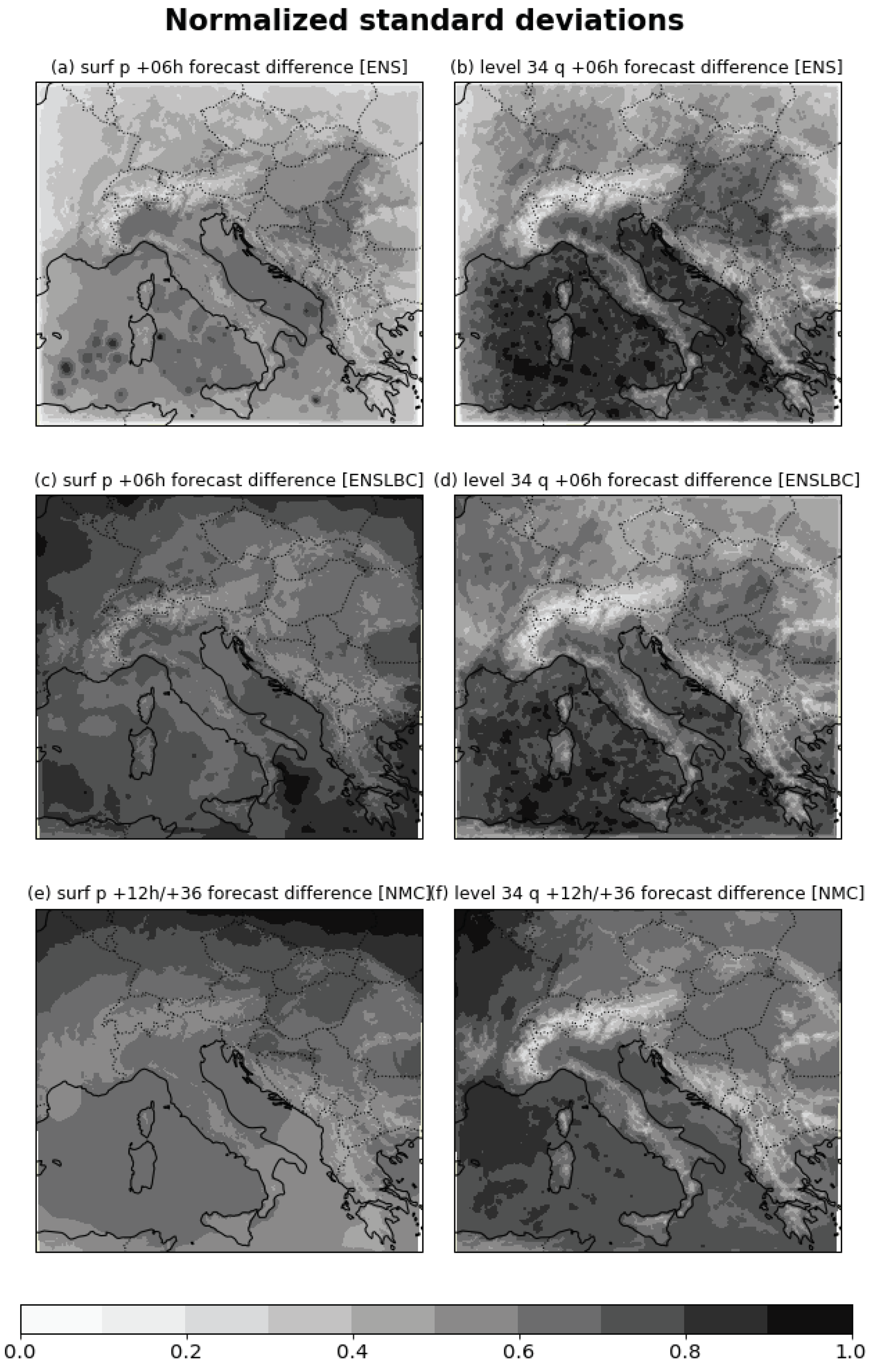
3.1.1. Geographical Distribution of the Standard Deviations

To address the characteristics of the estimated B matrices, the standard deviations (STD) in the grid-point space were computed and compared. In Figure 1 the normalized STD for the surface pressure and specific humidity at level 34 (approximately 500 hPa) of the samples used in B matrix estimation are plotted. The normalization was performed by dividing the STD by the maximum horizontal value of the STD. The maximum values of the STD were similar for the two ensemble experiments (ENS p: 0.6 hPa; ENSLBC p: 0.77 hPa; ENS q: 0.26 g/kg; and ENSLBC q: 0.29 g/kg) but were significantly larger for the NMC experiment (NMC p: 6.76 hPa and NMC q: 0.55 g/kg). The maximum STD values for the surface pressure and ensemble experiments were comparable to those found in [14], but they were larger than those of their NMC experiment (3.53 hPa for their NMC experiment). The patterns found in the STD maps could be explained by several overlapping effects, and they are discussed in the following text.

(a) Influence of the weather regime

Large STD were expected for the NMC and ENSLBC samples at the N and the NW part of the domain as synoptic disturbances were common in this area during the winter period used for obtaining samples. These disturbances influenced the faster spreading of information from the LBCs into the domain and decreased the predictability of the model state in this area. For the ENS, wider areas of low LBC STD were expected at the N and the NW part of the domain due to the stronger advection from the boundaries caused by synoptic disturbances. This is indeed true for the STD of the surface pressure in the ENS sample, where a small surface pressure STD could be found at all borders with the largest area of small STD at the N and NW parts of the domain. This effect was not as pronounced for the specific humidity. For the NMC, the largest pressure STD was found in the northern (N) part of the domain, and the largest STD of the humidity was at the W boundary of the domain. On the other hand, for the ENSLBC experiment, the larger STD of the surface pressure were found at all model boundaries with the largest amplitudes on the N, NW and S (SE) boundaries.

(b) Influence of the method used for obtaining the samples

As discussed at the end of Section 2, in data-poor areas, small forecast differences are expected for the NMC samples. This is one of the shortcomings of the NMC method because in this area, the background error should be higher as the analysis had less information to reduce the error locally. On the other hand, the STD in the data-poor area was expected to be higher for the ensemble differences, as in this area, there were no observations to anchor the analysis and the subsequent forecast. The observation density for the surface observations (also to some extent for upper-air observations) was small at the S part of the domain (mostly covered by sea); thus, lower NMC STD were expected in that area and higher for the ensemble samples. For both ensemble samples, the land-sea contrast was visible in the surface pressure and humidity STD fields with the higher values found over sea. A similar distribution could also be found for the upper-air temperature and wind fields (not shown). For the NMC samples, this land-sea contrast was not visible for the surface pressure and humidity, but it was clearly visible for the upper-air temperature and wind fields (not shown) with smaller STD values over sea.

(c) Influence of the LBCs

The influence of LBC perturbations was expected predominantly near the lateral boundaries of the domain with a larger affected area at the N due to the influence of the weather regime. As all the members of the ENS experiment had the same LBCs, the STD for the surface pressure was the lowest at the boundaries of the domain. This area of smaller STDs spread toward the center of the domain with the largest area of small STD at the N and NW of the domain. However, this area of small STD, although present, was not as noticeable for the humidity. Neglecting the LBC perturbation in the ENS experiment is deficient by construction, but it is an interesting setup to visualize the LBC influence in the surface pressure STD plot. In contrast, in the ENSLBC experiment, where perturbed LBCs were used, the largest surface pressure STDs were found at the edges of the domain (mainly at the N, NW and SE) from where they were decreasing toward the center of the domain. The humidity STD patterns were similar between the ENS and ENSLBC experiments. The influence of the LBC perturbations on the STD in the ENS (ENSLBC) experiment for the upper-air temperature fields (not shown) was similar to that for the surface pressure with the lowest (highest) STD at all domain boundaries. For both ensemble experiments, the wind field STD had a maximum in the central and the southern part of the domain (not shown). For the NMC samples, the geographical distribution of STD for the upper-air wind fields and temperature differed from that found in the ensemble experiments, with the maximum amplitude found in the N of the domain (not shown). For the NMC experiment, which also used different LBCs (from the IFS deterministic run) in the +12 and +36-hour model forecasts, the highest surface pressure STD were at the northern edge of the domain from where they were spreading southerly inside the domain. For the humidity, the largest STD were found at the western edge of the domain, and the overall pattern was different than that found for the ensemble methods. The LBCs that were used in the NMC experiment came from a deterministic IFS model run with a horizontal grid spacing of approximately 9 km, while the LBCs used in the ENSLBC experiment came from a coarser IFS ensemble with a horizontal grid spacing of approximately 18 km. A notable difference was found between the NMC and ENSLBC STD patterns, as higher NMC STD were found mainly in the N part of the domain, while for the ENSLBC effect of LBC perturbations was visible at all lateral boundaries. Noticeable differences in the horizontal grid spacing between the ALADIN-HR4 and IFS ensembles for the ENSLBC experiment could lead to discrepancies between the development of the model state in the host and driving model and influence the boundary area on all sides of the domain, but this assumption should be further investigated, which was not the aim of this paper.

Considering the previously mentioned effects, it is important to note that the specific humidity patterns of STD were rather similar between the two ensemble experiments. This could imply that humidity background errors were less sensitive to the LBC perturbations and thus more sensitive to analysis perturbations (the latter being the same in both ensemble experiments). The LBC perturbation influence on the standard deviations in the grid space was also discussed in [14], and it was found that the LBCs influenced a relatively small part of their domain while they influenced a relatively large part of the ALADIN-HR4 domain. Having a small horizontal domain of the model, with a large part influenced by LBC perturbations, and taking into account that during the estimation of the B matrix averages over the domain were used, LBC perturbations could have a considerable effect on the B matrix characteristics (increase of background-error variances and influence on background-error correlations).

Similar STD maps could be used in 3DVar, but this was not the case in the conducted experiments; we instead used them for diagnostic purposes.

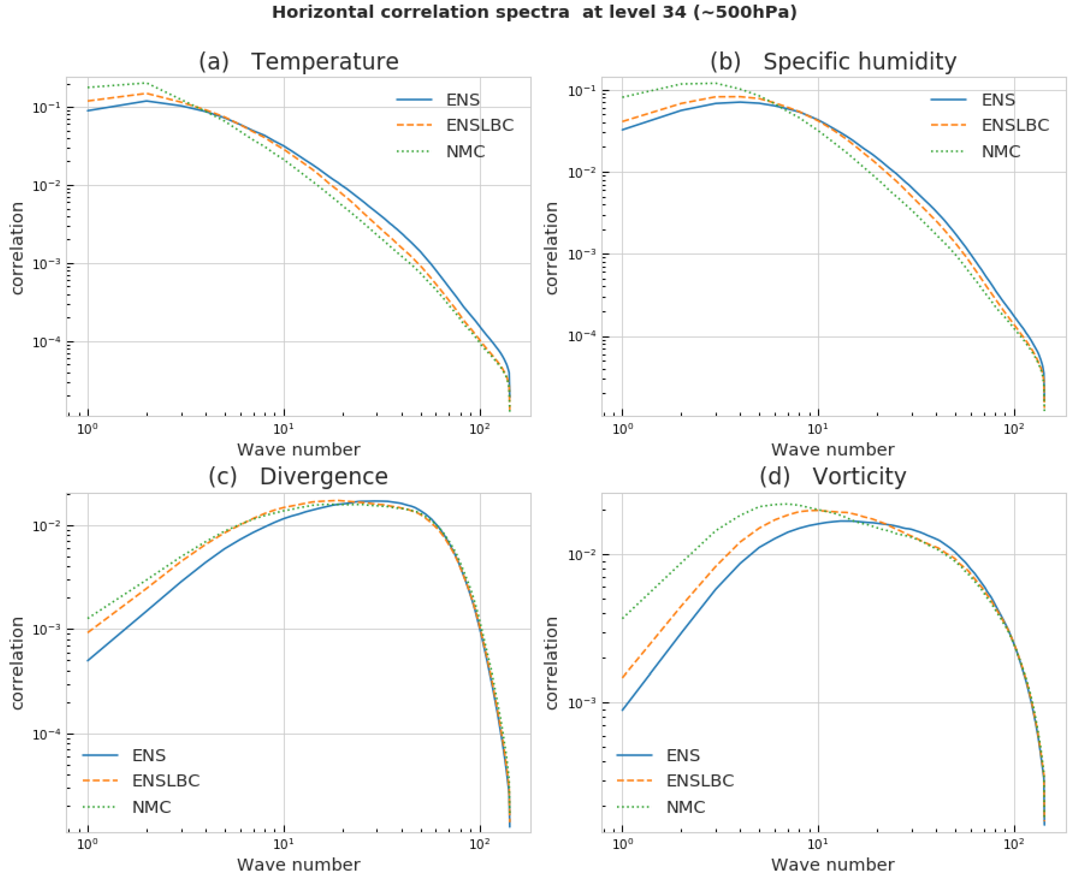
3.1.2. Horizontal Spectral Densities

The horizontal correlation spectra were obtained by normalizing the variance spectra by the total variance to compare the contributions of the different horizontal scales to the correlation function shape for the different experiments. The horizontally averaged variance spectra were calculated according to Equation (A3) of [32]. They are plotted for all control variables (surface pressure, temperature, specific humidity, vorticity and divergence) in Figure 2 (for vertical level 34, near 500 hPa).

The relative amount of the large-scale variance (small wave numbers) was the largest for NMC experiment, with the ENSLBC experiment in the middle and the ENS experiment with the smallest amount of large-scale variance. This result is consistent with findings in [13], where it was shown that the large-scale part of the spectrum was (i) decreased for the ensemble method compared to the NMC method because of the involvement of the analysis error instead of the analysis increments and the shorter forecast ranges in the evolution of the model state errors and (ii) increased for the NMC method due to the different LBCs used (as in ENSLBC). The shape of the correlation spectra was shifted toward the smaller scales (especially for the ENS method) for both ensemble methods compared to the NMC method, and this shift was more pronounced for the surface pressure, temperature, humidity and less pronounced for the divergence and vorticity. The difference between the shape of the correlation spectra for the ENSLBC and NMC experiments was found to be smallest for the divergence at all levels. The smallest difference between the correlation spectra of the ENSLBC and ENS experiments was found for the humidity. This result suggests that the LBC perturbations in the ENSLBC experiment have a small influence on the shape of correlation spectra of humidity background error. Similar shapes of the correlation functions and shifts to smaller scales for the ensemble method compared to NMC were also reported in previous research (e.g., [13,14]). For all experiments a shift of correlations spectra towards the large scales by going from the surface to the model top was noticed (not shown).

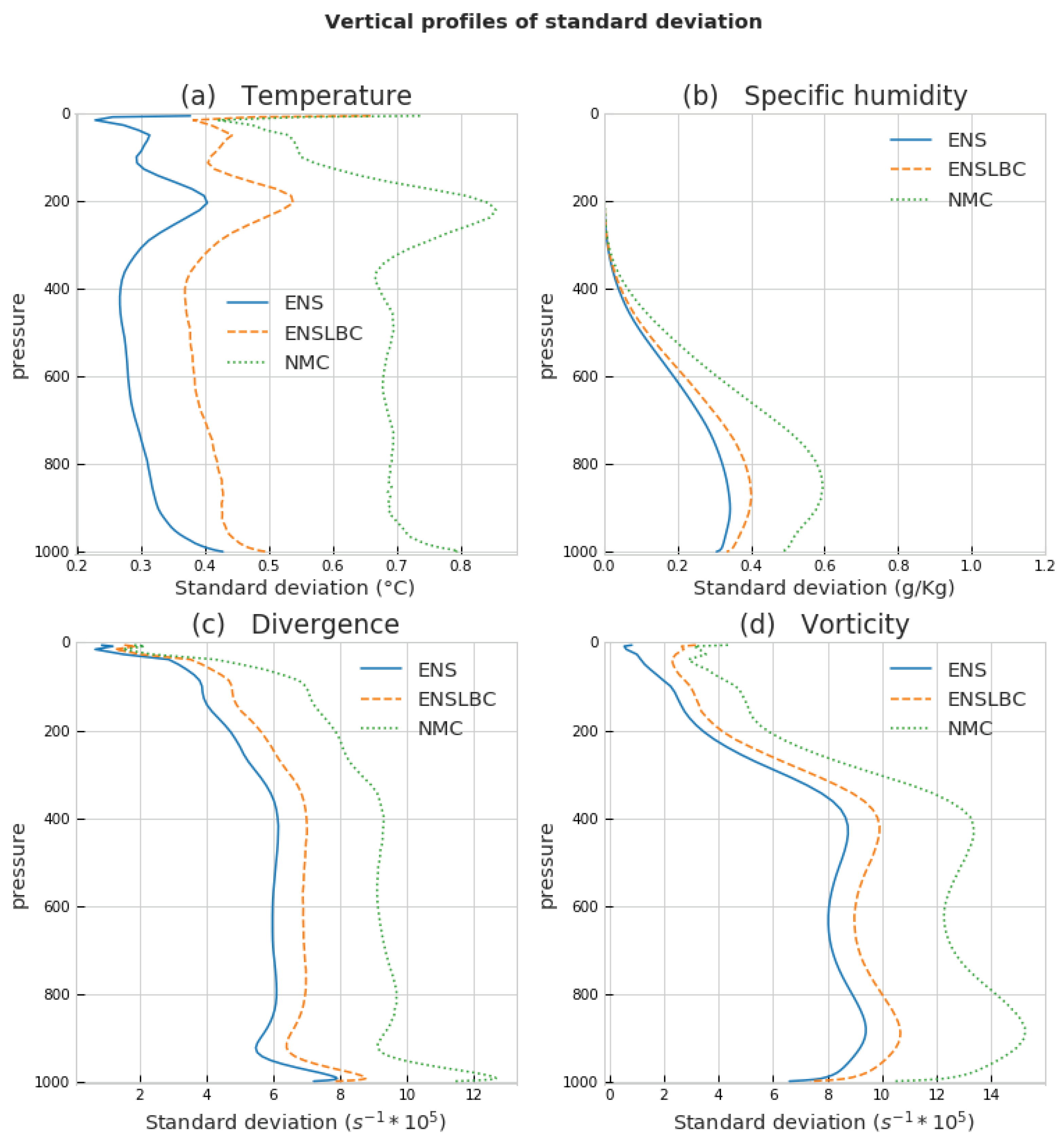
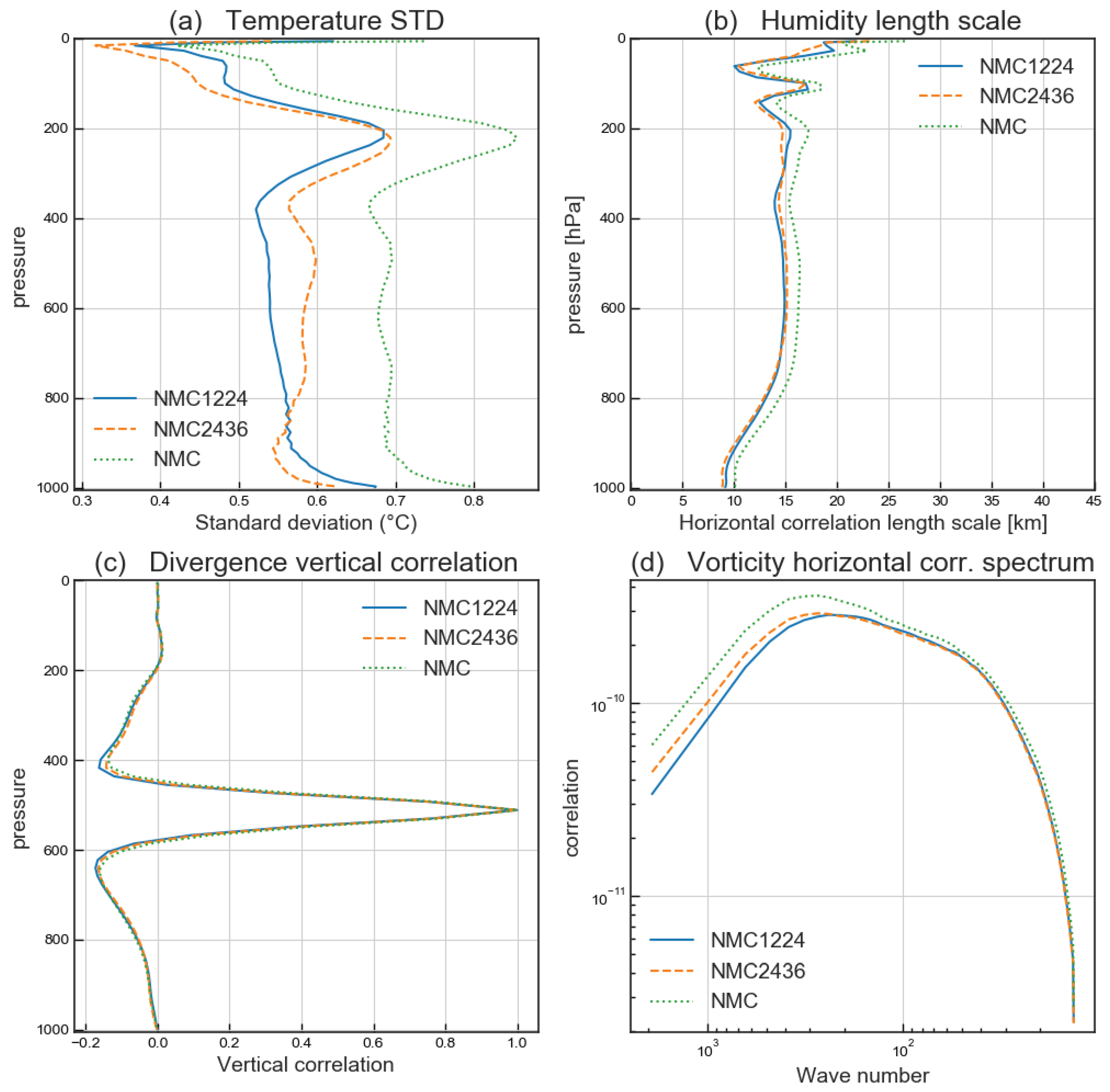
3.1.3. Standard Deviation

The vertical profiles of the horizontally averaged standard deviations for the temperature, specific humidity, vorticity, and divergence for the three experiments are plotted in Figure 3.

They were obtained from sum of variance contributions from different horizontal wave numbers at a given model level according to calculations shown in [32]. The largest standard deviations were found for the NMC experiment, while the smallest ones were for the ENS experiment (as it lacks spreads near model boundaries, by construction). The ENSLBC standard deviations were between those of the ENS and NMC experiments, which could be expected from the variance spectra discussed in Section 3.1.2. Additionally, the smallest difference between the two ensemble methods was for the specific humidity. It was also showed in [13,14] that using ensemble methods decreased the STD magnitude for all control variables compared to the NMC method. Although there is a clear distinction between values of STD for NMC and ensemble-based B matrices, those are usually scaled before using them in DA.

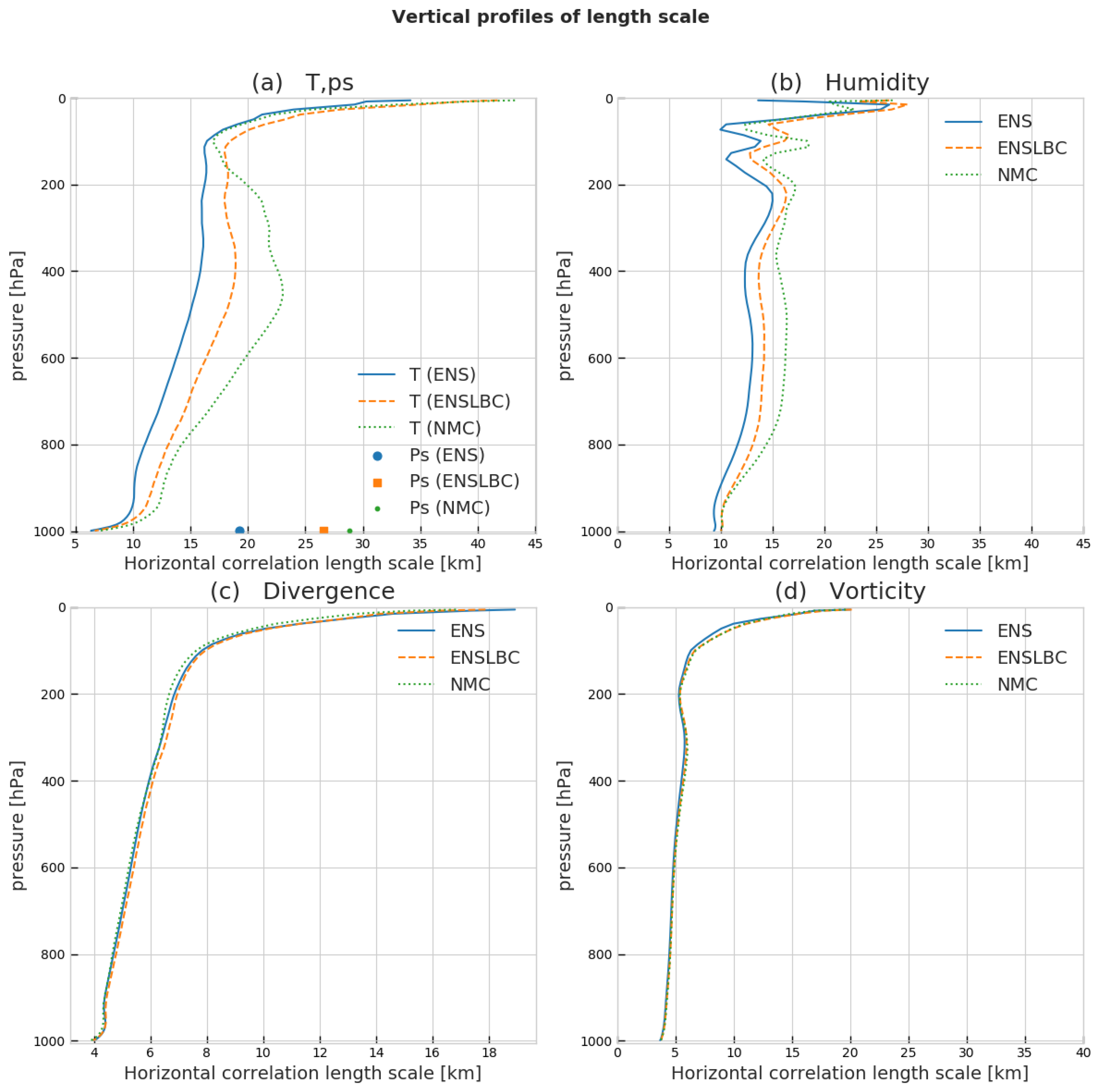
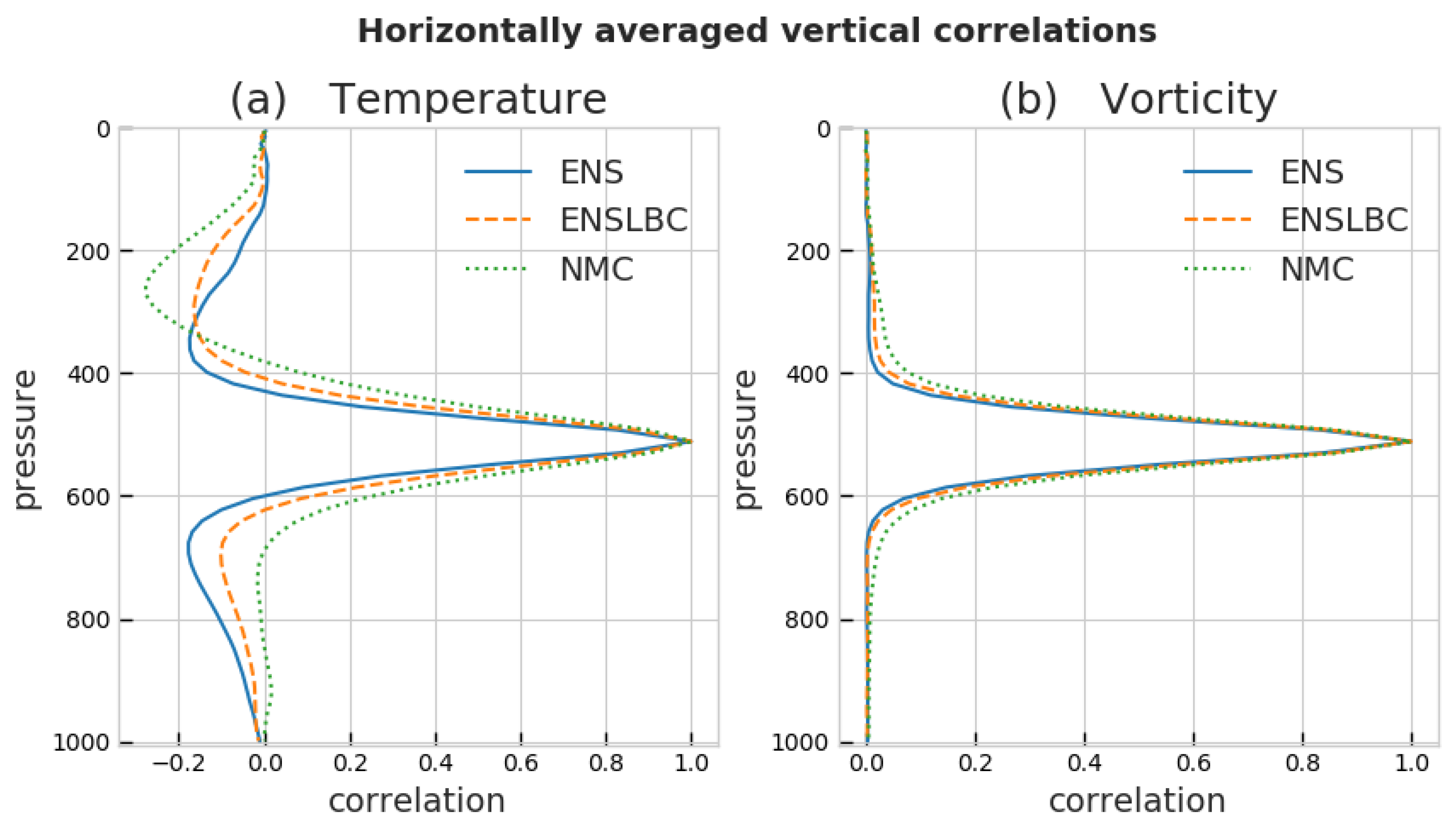
3.1.4. Horizontal and Vertical Correlations

The vertical profiles of the horizontal correlation length scales were estimated as in [32] and are plotted in Figure 4.

The horizontal correlation length scale at a given level is inversely proportional to the variance spectrum multiplied by the square of the wave number. Such a formulation puts weight on the short scale correlations, which is the reason the correlation length scales are small in terms of the absolute values. Therefore, because of the tendency of the correlation spectra to shift to large scales when going to higher levels, increase in the length scale with height is expected. This was the case for the temperature, vorticity and divergence, while the correlation length scale was noisy for humidity above 200 hPa (probably because there is only little humidity at this level). The largest differences among the correlation length scales for the different experiments were found for the temperature and specific humidity, while for the vorticity and divergence, the differences were negligible. The highest correlation length scale amplitudes were for the NMC experiment and the smallest for the ENS experiment with the ENSLBC values in between. The shape of the correlation length scale vertical profile was more similar for the two ensemble methods for the temperature and humidity compared to that of the NMC method.

The horizontal correlation lengths were comparable with those of previous research for models with a similar horizontal grid spacing (e.g., [18]) except for shorter values of the horizontal correlation length in stratospheric levels (especially for the vorticity and divergence). The decrease in the length scales for the ENS and ENSLBC experiments compared to that of the NMC experiment agreed with the decrease in the variance at the large scales, as discussed in Section 3.1.2. The vertical profiles of the vertical correlations were calculated by averaging the vertical covariances over the horizontal wave numbers, and they are plotted with reference to model level 34 (approximately 500 hPa) in Figure 5 for the temperature and vorticity.

The NMC experiment had the broadest vertical correlations, while the sharpest one was for the ENS experiment. Additionally, the ENS and ENSLBC experiments resulted in more similar correlation shapes compared to that of the NMC experiment.

The vertical profiles show that for the temperature negative correlations (up to −0.25) were found above the maximum correlation near 500 hPa. This may reflects the vertical structure of the upper-level thoughts in the mid-latitudes, where upper-level tropospheric cold air is associated with a decrease of the tropopause and a warming of the air above it (e.g., [34]). Similar results are found below 500 hPa, albeit not as significant and consistent. While the shape of the correlation profile of the temperature was rather symmetrical above level 34 (approximately 500 hPa) for the ensemble experiments, negative correlations were found mainly above that level for the NMC experiment. Similar asymmetric features within the NMC temperature correlations were also found in [14].

The diagnostic study presented above suggest that the ensemble-based B matrix is better adapted for use in the LAM DA system because it emphasizes more on the small scales than the NMC B matrix. The importance and influence of the LBC perturbations was demonstrated with the ENS and ENSLBC experiments showing that the LBC perturbations mainly influenced the large scale for all control variables with the exception of the humidity, where the influence of the LBC perturbation is small. One of the driving ideas behind this work was to compare the ensemble method with NMC method that was used to estimate the operational B matrix, but to do the sampling for the same period as ENS/ENSLBC. Therefore, 36- and 12-hour forecast differences were used. The choice of 24 hour staggered forecast is usually made with aim to avoid errors in modeling of the diurnal cycle, but different choices have been made in previous literature (36- and 12-hour as in e.g., [13,35] or 48- and 24-hour as in [14], or 24- and 12-hour as in e.g., [7,8]). As forecasts used in NMC method incorporate longer forecast ranges than forecast used for obtaining background, adjustment to statistics is usually made with aim to scale resulting variances. As discussed in Section 2.2 and in [13] longer forecast ranges and involvement of analysis increments instead of analysis errors differences influences properties of NMC B matrix. In order to assess degree at which analysis increments and longer forecast ranges influence NMC B matrix characteristics, two additional NMC B matrices were estimated, using 36- and 24-hour forecast differences (NMC2436) and using 24- and 12-hour forecast differences (NMC1224). Comparison of NMC1224 and NMC2436 enables us to assess influence of longer forecast ranges, while comparison of NMC1224 and NMC enables us to assess influence of accumulation of analysis increments (8 in NMC and 4 in other two experiments). Similar diagnostic plots were made as before and some results are shown in Figure 6.

Results indicate that for standard deviation, length scale and vertical correlation more pronounced differences among experiments were found for temperature and humidity than for vorticity and divergence. Largest differences for divergence and vorticity were found for large-scale part of horizontal correlation spectrum where highest values were found for NMC experiment (e.g., Figure 6c). Overall results clearly show (e.g., Figure 6a,b,d) that accumulation of analysis increments influences statistics more than longer forecast ranges. Although, as shown, choice of forecast staggering can influence NMC B matrix characteristics, still differences between NMC and ensemble-based B matrix are more pronounced. In the following section, the impact of using NMC and ENSLBC B matrices on the analysis and quality of forecasts was tested. Because the ENS B matrix was only used to diagnose the influence of LBCs, it was left out in further analysis.

3.2. Impact on the Analysis and Forecast

Two ALADIN-HR4 DA cycles with 6-hour cycling were set up during June 2017, where B matrices, calculated from the ENSLBC and NMC experiments, were used. The DA cycle was the same as that used in the operational runs (Section 2.1), except that 6-hour cycling was used here. Two DA cycles provided an initial “condition” file for a 72-hour forecast starting at 00 UTC. No filtering method (e.g., digital filter initialization) was applied before model integration. The filtering step was omitted to avoid small scale structures that are the result of the analysis being misinterpreted as noise. To reduce the noise during a model spin-up, space-consistent coupling was used. Space-consistent coupling refers to a setup where the first LBC file was the same as the initial condition file (coming from the ALADIN-HR4 assimilation cycle). Prior to setting up DA cycles used for initialization of forecast, one month of 6 hourly cycling was performed for both experiments and tuning of the B matrices was conducted by using innovations as proposed by [36]. As in [35] the misfit ratio between vertical averages of predefined and diagnosed standard deviations was computed for temperature, specific humidity and kinetic energy (the squared average of u and v wind components). No variable dependent correction was applied, rather the average misfit ratio was calculated as average over mentioned variables and used for the overall tuning.

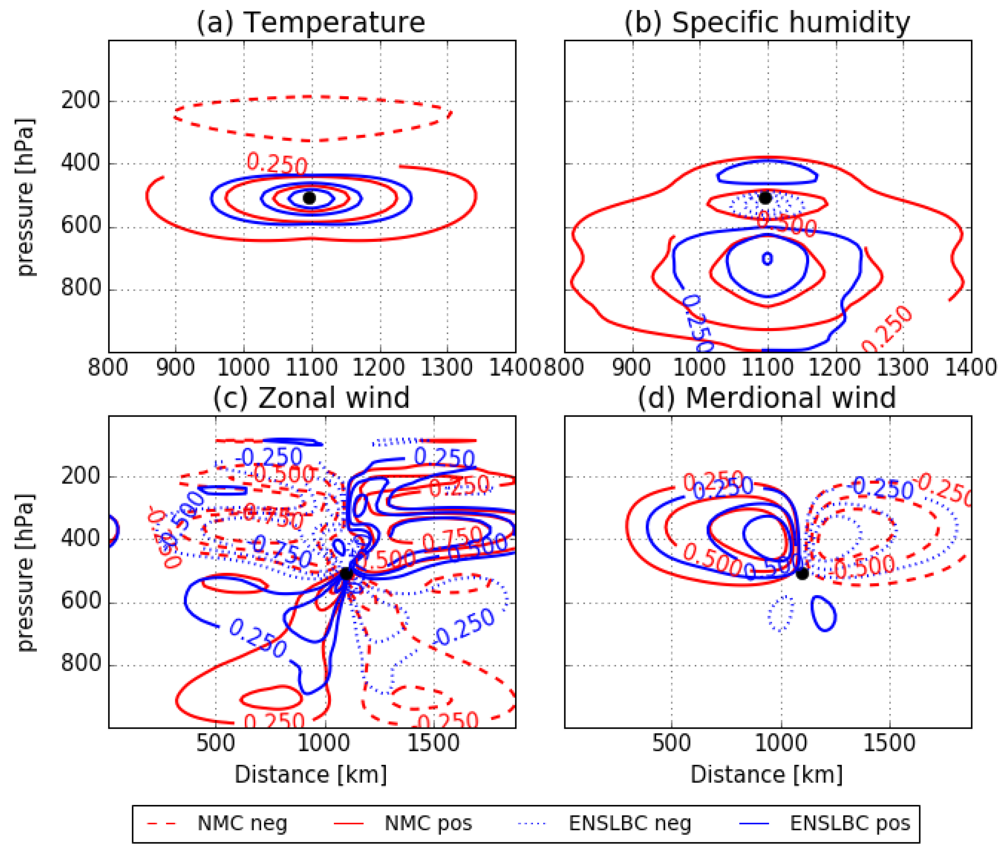
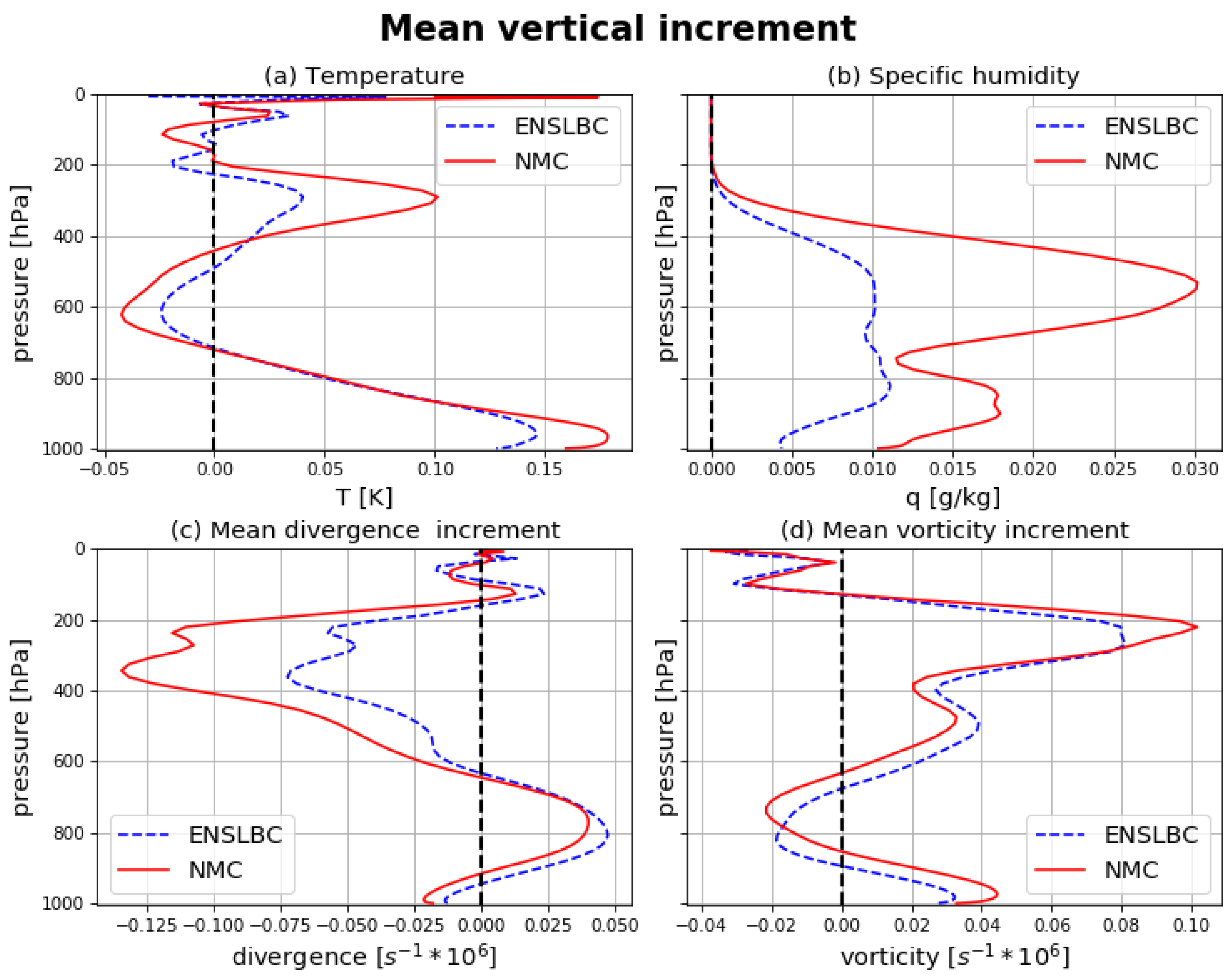
3.2.1. Impact on the Analysis

To test the influence of the different B matrices on the analysis, two single-observation experiments were performed with a temperature innovation of 1 K from radiosonde observations at approximately 500hPa and horizontally located at the model grid-point near the town of Zagreb, Croatia. The increments were normalized by their respective maximum values. The vertical zonal cross section through the location of observation of the normalized analysis increment for the temperature, specific humidity and two wind components is plotted in Figure 7.

The resulting increments for the two B matrices differed both in shape and spatial extent from the observation location. Sharper increments for the ENSLBC B matrix were clearly visible for all variables where the 0.5 contour lines differed by 50–200 km in extension for the two experiments. Except for the sharpness, the differences in the sign of the increment at certain places between the two experiments were noticed in all figures. This was most pronounced for the humidity, where a strong negative increment was present near the observation point for the ENSLBC experiment, while it was completely missing in the NMC experiment. Similar differences were also found for at horizontal cross section plot of the normalized analysis increments at model level near 500 hPa (not shown).

The influence on the analysis was also tested by averaging the increments horizontally by the model level and in time over all assimilation cycles in June 2017, and the results for the temperature, specific humidity, divergence and vorticity are shown in Figure 8.

The shape of the temperature increments is similar for both experiments, but the warming (below 900 hPa, and between 400 and 200 hPa) and cooling (approximately 600 hPa) is more pronounced for the NMC experiment. The vorticity increments were also rather similar, with slight differences in the location and intensity of the extremes. Larger differences were found for the divergence between 600 and 200 hPa. The largest differences were for the humidity, where moistening was present in both experiments, but the shape of the mean vertical increment was quite different between the two experiments.

The fit of the analysis to the observation was assessed by calculating the bias and root-mean-square error (RMSE) against radiosonde observations for the month of July 2017 and is presented in Figure 9.

The overall better fit to the observations was for the ENSLBC experiment, especially for the wind. Smaller RMSE but slightly higher bias of NMC compared to ENSLBC was found for geopotential between 800 and 400 hPa. The moistening in the NMC experiment between 800 and 400 hPa, as shown in Figure 8 drove the model away from the observations, which was visible on the bias score for the specific humidity.

The beginning of model integration could be affected by the imbalances produced by the analysis, and the effect of these imbalances (spin-up effect) could be noticed in the surface pressure field. To assess the degree of balance within the analyses produced using different B matrices, the mean and root-mean-square of the surface pressure tendency over the domain were calculated. Statistics for the surface pressure tendencies were calculated for every time step (180 sec) during the 6-hour forecasts inside the DA cycle, and the average over several forecasts (11 forecasts) is plotted in Figure 10.

High values for both the mean and root-mean-square at the beginning of the forecasts indicated that the model was adjusting during the first three hours of forecasting in both experiments. Nevertheless, smaller values were found for the ENSLBC experiment compared to the NMC experiment, thus most probably showing more balanced initial conditions. Even though, variances of both B matrices were rescaled, it appears from Figure 8 that somewhat larger amplitude increments were present for NMC B matrix and this could also influence spin-up. To test this, we have re-run DA cycle with NMC B matrix for same period (11 forecasts), but we have inflated standard deviations for NMC B matrix (with same factor for all variables) for approximately 60%. Resulting pressure tendencies were only slightly different (not shown) from results obtained for NMC, which indicates that more balanced initial conditions and not amplitude of analysis increments decreased spin-up.

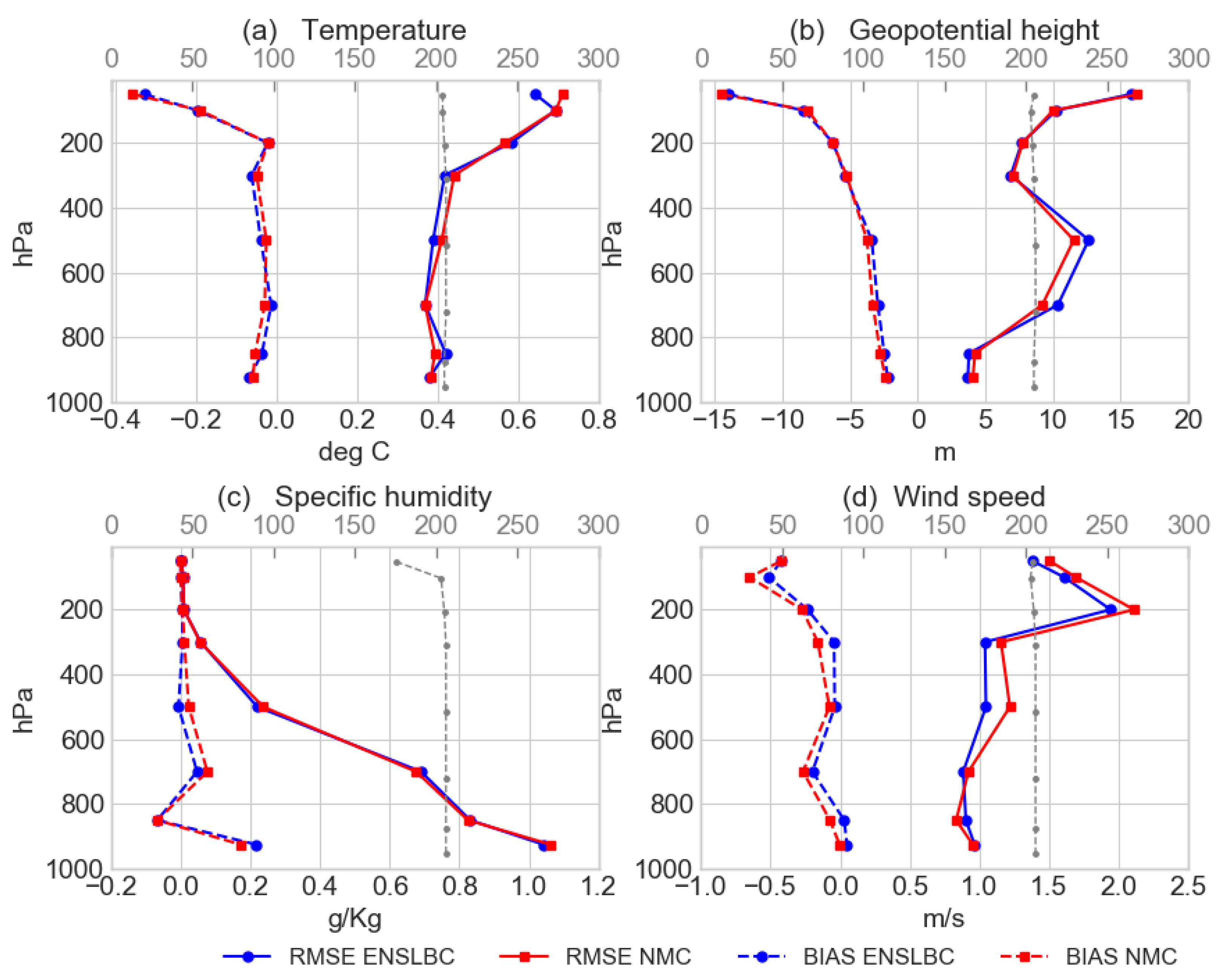
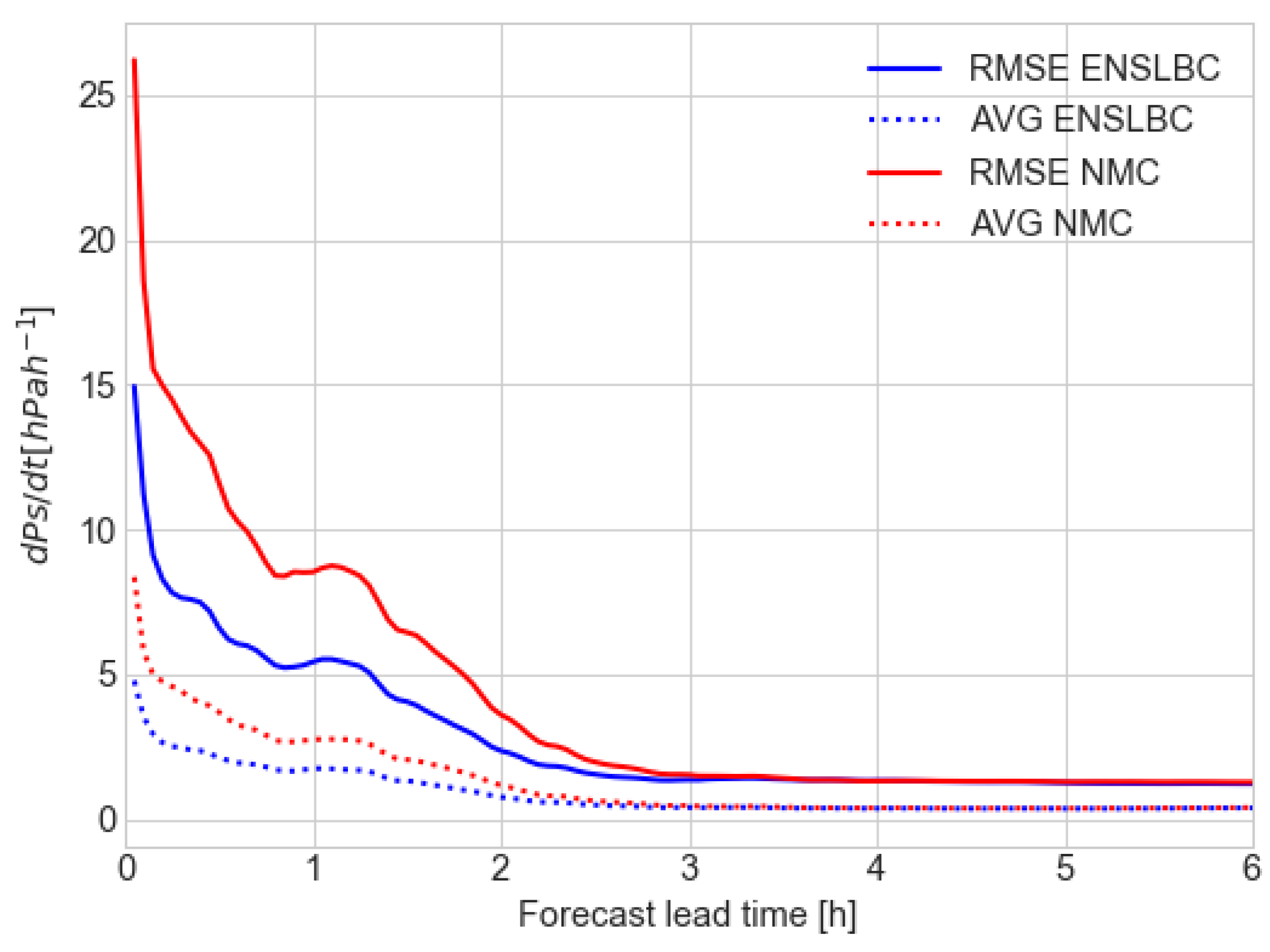
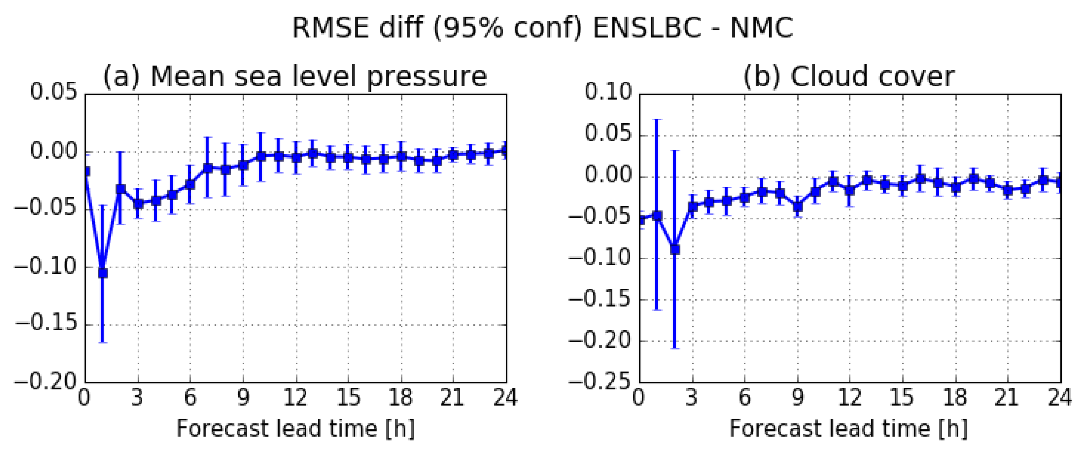
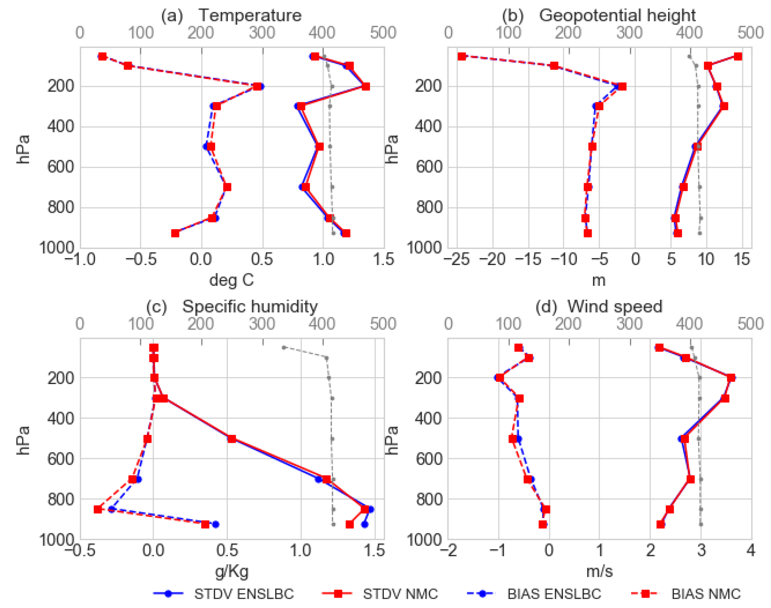
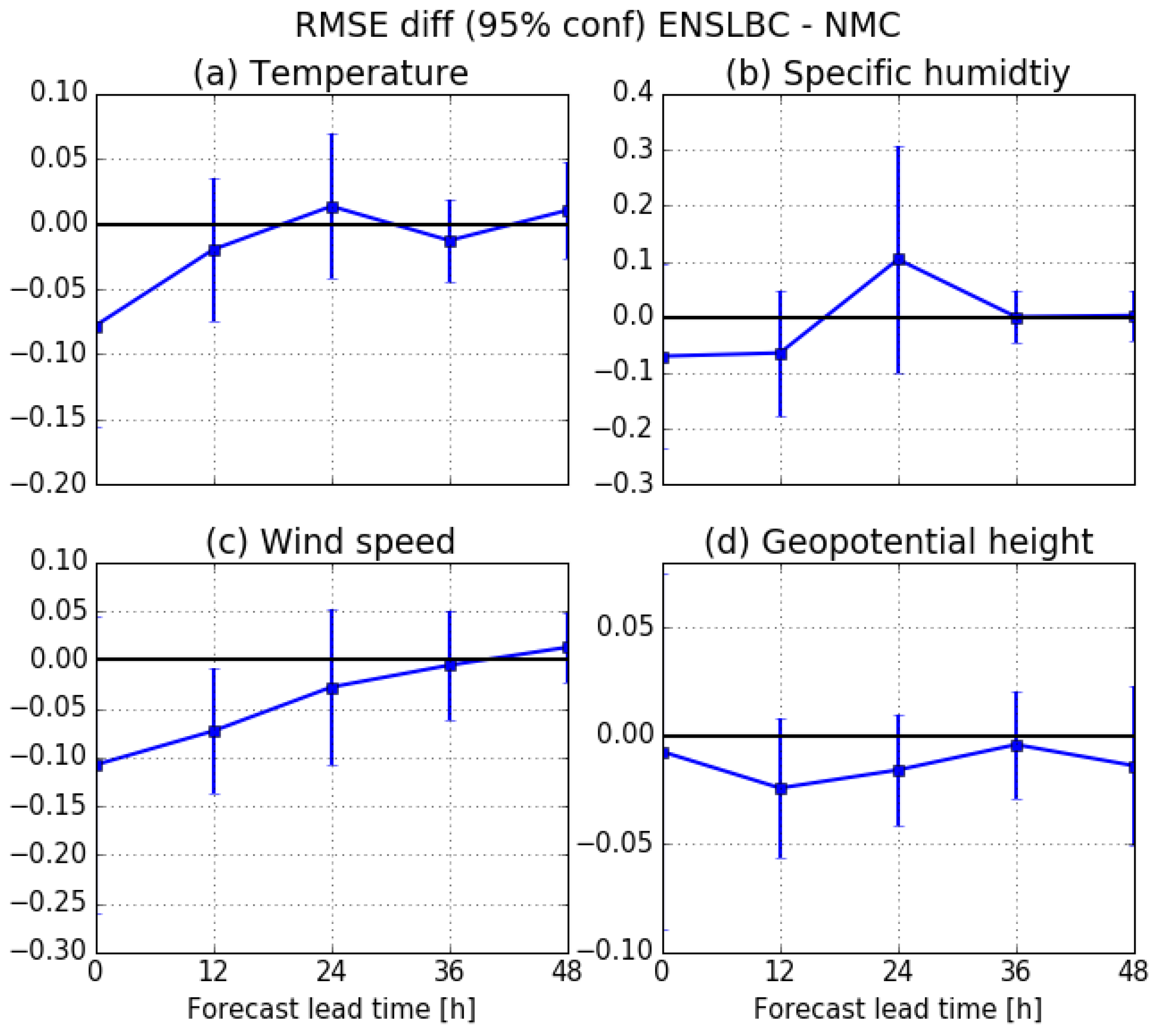
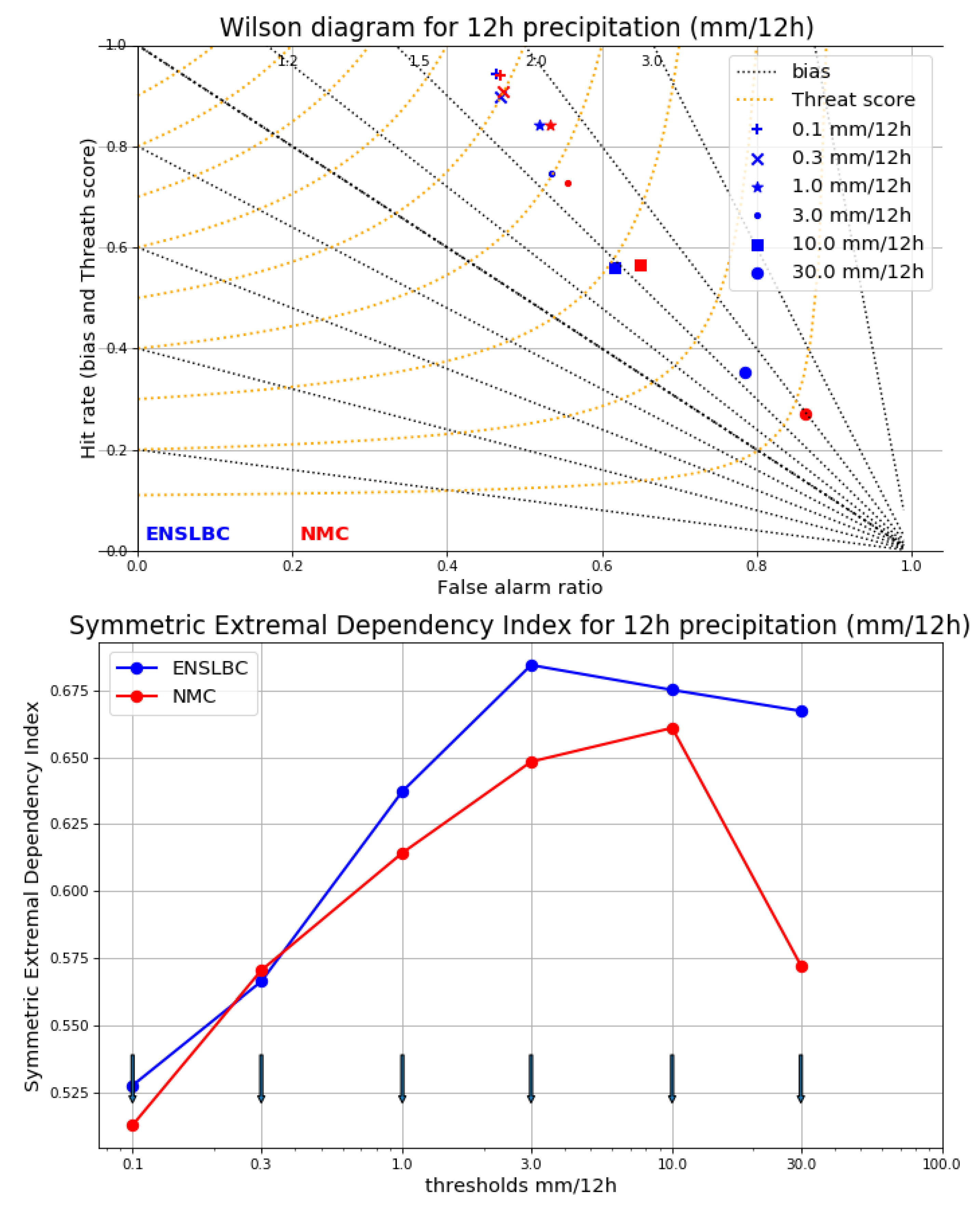
3.2.2. Impact on The Forecast Quality

The quality of the forecasts started from the ALADIN-HR4 DA system using different B matrices was assessed by comparing the forecasts with in situ data from surface and radiosonde observations during June 2017. To determine if the differences between the experiments were statistically significant, a t-test was used at the 95% confidence level.

For the surface parameters, the differences between the experiments were negligible, except for the mean sea level pressure (MSLP) and total cloudiness. Figure 11 shows the normalized mean root-mean-square difference between the ENSLBC and NMC experiments for the MSLP and for the cloud cover for June 2017 and for both experiments.

The results suggest that the MSLP forecast was better in the first 6 hours for the ENSLBC experiment, which was likely related to the higher degree of balance in the ENSLBC experiment as shown in Section 3.2.1. The total cloud cover was better for the ENSLBC experiment for the first 12 hours of the forecast (only for two lead times they were not statistically significant). Similar verification scores for most parameters but different ones for the humidity could be connected with the results from Section 3.2.1, where it was shown that the most pronounced differences between the two B matrices and their effect on the analysis were found for the humidity.

The vertical profiles of the bias and STD were calculated by comparing the model forecasts with radiosonde observations at 12 UTC (using the +12- and +36-hour forecasts started at 00 UTC) for June 2017 and are shown in Figure 12.

The results are rather similar for both experiments, with small differences indicating slightly better results for the ENSLBC experiment. Nevertheless, as demonstrated, for example, for the verification of the forecasts at 500 hPa in Figure 13, these differences were mostly not significant, and if they were it was only for certain cases depending on the model level, the forecast hour and the model variable.

For the precipitation, the point-based verification where the model output was compared to the rain gauge measurements over the domain was performed and the verification statistics were calculated from contingency tables. To compare the model results with the 12-hour accumulated precipitation from a rain gauge that measured the precipitation at 18 UTC, the model precipitation accumulation between the +6 and +18 hour forecast was used, and the verification results are shown in Figure 14.

The Wilson diagram (one variant of the performance diagram [37]) aggregates several verification measures with the ideal score in the upper left corner of the diagram. The scores suggested that for the two highest precipitation thresholds, better results were obtained for the ENSLBC experiment. Additionally, the symmetric extremal dependence index (SEDI) [38], which is base-rate-independent and thus suited for the verification of rare events, was calculated and plotted on the bottom row of Figure 14. Again, the ENSLBC experiment outperformed the NMC experiment to a certain extent. This is especially the case for higher precipitation thresholds. The threat score already shows the ENSLBC predominance for high precipitation event thresholds, but this result is important because the SEDI, unlike the threat score, is not base-rate-dependent score. Therefore, it confirms the ENSLBC high precipitation event forecasting predominance independently on the underlying climatology.

4. Summary and Conclusions

Climatological B matrices for the ALADIN-HR4 model were estimated using three error simulation techniques. The characteristics of these B matrices, along with their influence on the analysis and quality of the forecast, were investigated using spectral and moment-based evaluation in diagnostic comparison, single-observation experiments and full observation forecast experiments. The first technique used was the standard NMC method. The second and third approaches obtained samples of forecast differences by using the EDA system with a cycling frequency of 6 hours and with 2 members. To test the influence of LBC perturbations, one EDA system had the same LBCs for all members (from the deterministic IFS run), while the other had perturbed LBCs from the global IFS ensemble. For all experiments, the sampling was consistently performed over the same period of almost 3 months.

The examination of the forecast differences using the geographical distribution of the normalized standard deviation showed that neglecting LBC perturbations led to unrealistically small standard deviations near the domain boundaries. It also showed that for the specific humidity, the smallest differences were between the ENS and ENSLBC experiments, which suggest that the humidity field is more sensitive to the method used to sample the forecast error than to LBCs. For the other variables, especially for the surface pressure and temperature, a notable influence on the standard deviation amplitude came from the LBC perturbations. More importantly, this influence spread over a significant portion of the relatively small ALADIN-HR4 domain. Considering that the B matrix was estimated from temporal and the domain averages, the influence of the LBC perturbations could dominate other sources of background errors. The influence of LBC perturbations was confirmed by diagnostic comparison, where it was shown that the contribution of the large scales to the shape of the correlation function for the ENSLBC experiment was enhanced and had amplitudes closer to those of the NMC experiment. Nevertheless, the shape of the correlation functions from the ENSLBC experiment was shifted to smaller scales compared to the NMC experiment. The ensemble B matrices were further characterized by smaller standard deviations, shorter horizontal length scales and sharper vertical correlations compared to the B matrix derived using the NMC method, which agrees with previous research results. The influence of the ENSLBC and NMC B matrix on the analysis was tested by performing a single-observation experiment, calculating the mean analysis increments, calculating the fit of the analysis to the observations and by assessing the influence of the B matrix on the internal model balances in the analysis.

The single-observation experiment showed that the ENSLBC analysis increments had a smaller spatial extent with a shape that was more or less similar for all control variables compared to the NMC experiment. The most pronounced differences were found for the specific humidity. This agreed well with the mean analysis increments, which differed between the NMC and ENSLBC experiments, mostly for the specific humidity, showing apparently excessive (from the fit of the analysis to the observations) moistening of one part of the atmosphere. A clear benefit of using the ENSLBC B matrix was demonstrated by the model spin-up, where it was shown that less imbalance was present in the analysis using the ENSLBC method. For both experiments, approximately 3 hours were needed for the model to adjust to the internal balance, and the degree of imbalance was relatively smaller for the ENSLBC experiment.

The quality of the forecast initialized from the local DA system that used different B matrices was assessed by comparing the forecast with in situ data from surface and radiosonde observations during June 2017. The verification results showed that the choice of the B matrix had a small influence on the forecast of the surface parameters. Nevertheless, a statistically significant improvement of the ENSLBC experiment compared to the NMC experiment was found for the mean sea level pressure and for the cloud cover in the first 6–12 hours of the forecast. The upper-air verification scores were generally not significant, although some slightly better statistics were obtained for the ENSLBC experiment. A comparison of the 12-hour “accumulation” precipitation forecasts (accumulation between +06 and +18-hour forecast started at 00UTC) was performed against rain gauge measurements (that measure precipitation at 18UTC), and better results for the precipitation thresholds of 10 and 30 mm/12 h were obtained for the ENSLBC experiment.

The comparison of the NMC and ENSLBC B matrices in a diagnostic sense and based on the influence on the analysis and quality of the forecast showed that using the ENSLBC B matrix in the variational DA system would be preferred. For all performed comparisons, the most marked differences were noticed for the specific humidity or variables related to it (e.g., cloudiness, precipitation). Smaller, if any, improvement was found for the other variables. With the increased availability of humidity and precipitation information, sensitivity found in humidity fields needs to be further explored, as future plans involve assimilation of humidity observations derived from radar data delivered by OPERA radar project [39].

References

1. Kalnay, E. Atmospheric Modeling, Data Assimilation and Predictability; Cambridge University Press: Cambridge, UK, 2003. [Google Scholar]
2. Bannister, R. A review of operational methods of variational and ensemble-variational data assimilation. Q. J. R. Meteorol. Soc. 2017, 143, 607–633. [Google Scholar] [CrossRef]
3. Gustafsson, N.; Janjić, T.; Schraff, C.; Leuenberger, D.; Weissmann, M.; Reich, H.; Brousseau, P.; Montmerle, T.; Wattrelot, E.; Bučánek, A.; et al. Survey of data assimilation methods for convective-scale numerical weather prediction at operational centres. Q. J. R. Meteorol. Soc. 2018, 144, 1218–1256. [Google Scholar] [CrossRef]
4. Parrish, D.F.; Derber, J.C. The National Meteorological Center’s spectral statistical-interpolation analysis system. Mon. Weather Rev. 1992, 120, 1747–1763. [Google Scholar] [CrossRef]
5. Fisher, M. Background error covariance modelling. In Proceedings of the Seminar on Recent Development in Data Assimilation for Atmosphere and Ocean, Reading, UK, 8–12 September 2003; pp. 45–63. [Google Scholar]
6. Errico, R.M.; Privé, N.C.; Gu, W. Use of an OSSE to evaluate background-error covariances estimated by the NMC method. Q. J. R. Meteorol. Soc. 2015, 141, 611–618. [Google Scholar] [CrossRef]
7. Sun, J.; Wang, H.; Tong, W.; Zhang, Y.; Lin, C.Y.; Xu, D. Comparison of the impacts of momentum control variables on high-resolution variational data assimilation and precipitation forecasting. Mon. Weather Rev. 2016, 144, 149–169. [Google Scholar] [CrossRef]
8. Xu, D.; Shen, F.; Min, J. Effect of Adding Hydrometeor Mixing Ratios Control Variables on Assimilating Radar Observations for the Analysis and Forecast of a Typhoon. Atmosphere 2019, 10, 415. [Google Scholar] [CrossRef]
9. Široká, M.; Fischer, C.; Cassé, V.; Brožkova, R.; Geleyn, J.F. The definition of mesoscale selective forecast error covariances for a limited area variational analysis. Meteorol. Atmos. Phys. 2003, 82, 227–244. [Google Scholar] [CrossRef]
10. Pereira, M.B.; Berre, L. The use of an ensemble approach to study the background error covariances in a global NWP model. Mon. Weather Rev. 2006, 134, 2466–2489. [Google Scholar] [CrossRef]
11. Buehner, M. Ensemble-derived stationary and flow-dependent background-error covariances: Evaluation in a quasi-operational NWP setting. Q. J. R. Meteorol. Soc. 2005, 131, 1013–1043. [Google Scholar] [CrossRef]
12. Ştefănescu, S.E.; Berre, L.; Pereira, M.B. The evolution of dispersion spectra and the evaluation of model differences in an ensemble estimation of error statistics for a limited-area analysis. Mon. Weather Rev. 2006, 134, 3456–3478. [Google Scholar] [CrossRef]
13. Berre, L.; Ecaterina Ştefănescu, S.; Belo Pereira, M. The representation of the analysis effect in three error simulation techniques. Tellus A 2006, 58, 196–209. [Google Scholar] [CrossRef]
14. Storto, A.; Randriamampianina, R. Ensemble variational assimilation for the representation of background error covariances in a high-latitude regional model. J. Geophys. Res. Atmos. 2010, 115. [Google Scholar] [CrossRef] [Green Version]
15. Fischer, C.; Montmerle, T.; Berre, L.; Auger, L.; Ştefănescu, S.E. An overview of the variational assimilation in the ALADIN/France numerical weather-prediction system. Q. J. R. Meteorol. Soc. 2005, 131, 3477–3492. [Google Scholar] [CrossRef]
16. Brousseau, P.; Berre, L.; Bouttier, F.; Desroziers, G. Background-error covariances for a convective-scale data-assimilation system: AROME–France 3D-Var. Q. J. R. Meteorol. Soc. 2011, 137, 409–422. [Google Scholar] [CrossRef]
17. Berre, L.; Monteiro, M.; Pires, C. An impact study of updating background error covariances in the ALADIN-France data assimilation system. J. Geophys. Res. Atmos. 2013, 118, 11–075. [Google Scholar] [CrossRef]
18. Bučánek, A.; Brožková, R. Background error covariances for a BlendVar assimilation system. Tellus A Dyn. Meteorol. Oceanogr. 2017, 69, 1355718. [Google Scholar] [CrossRef]
19. Monteiro, M.; Berre, L. A diagnostic study of time variations of regionally averaged background error covariances. J. Geophys. Res. Atmos. 2010, 115. [Google Scholar] [CrossRef] [Green Version]
20. Ménétrier, B.; Montmerle, T.; Berre, L.; Michel, Y. Estimation and diagnosis of heterogeneous flow-dependent background-error covariances at the convective scale using either large or small ensembles. Q. J. R. Meteorol. Soc. 2014, 140, 2050–2061. [Google Scholar] [CrossRef]
21. Buehner, M.; Gauthier, P.; Liu, Z. Evaluation of new estimates of background-and observation-error covariances for variational assimilation. Q. J. R. Meteorol. Soc. 2005, 131, 3373–3383. [Google Scholar] [CrossRef]
22. Hacker, J.; Draper, C.; Madaus, L. Challenges and Opportunities for Data Assimilation in Mountainous Environments. Atmosphere 2018, 9, 127. [Google Scholar] [CrossRef]
23. ALADIN International Team. The ALADIN project: Mesoscale modelling seen as a basic tool for weather forecasting and atmospheric research. WMO Bull. 1997, 46, 317–324. [Google Scholar]
24. Termonia, P.; Fischer, C.; Bazile, E.; Bouyssel, F.; Brožková, R.; Bénard, P.; Bochenek, B.; Degrauwe, D.; Derkova, M.; El Khatib, R.; et al. The ALADIN System and its Canonical Model Configurations AROME CY41T1 and ALARO CY40T1. Geosci. Model Dev. Discuss. 2017, 2017, 1–45. [Google Scholar] [CrossRef]
25. Gerard, L.; Piriou, J.M.; Brožková, R.; Geleyn, J.F.; Banciu, D. Cloud and precipitation parameterization in a meso-gamma-scale operational weather prediction model. Mon. Weather Rev. 2009, 137, 3960–3977. [Google Scholar] [CrossRef]
26. Geleyn, J. Use of a modified Richardson number for parameterizing the effect of shallow convection. J. Meteorol. Soc. Jpn. Ser. II 1986, 64, 141–149. [Google Scholar] [CrossRef]
27. Tudor, M.; Ivatek-Šahdan, S.; Stanešić, A.; Horvath, K.; Hrastinski, M.; Odak Plenković, I.; Bajić, A.; Kovačić, T. Changes in the ALADIN operational suite in Croatia in the period 2011-2015. Hrvatski Meteorološki Časopis 2016, 50, 71–89. [Google Scholar]
28. Stanešić, A. Assimilation system at DHMZ: Development and first verification results. Hrvatski Meteorološki Časopis 2011, 44, 3–17. [Google Scholar]
29. Donlon, C.J.; Martin, M.; Stark, J.; Roberts-Jones, J.; Fiedler, E.; Wimmer, W. The operational sea surface temperature and sea ice analysis (OSTIA) system. Remote Sens. Environ. 2012, 116, 140–158. [Google Scholar] [CrossRef]
30. Ivatek-Šahdan, S.; Stanešić, A.; Tudor, M.; Plenković, I.O.; Janeković, I. Impact of SST on heavy rainfall events on eastern Adriatic during SOP1 of HyMeX. Atmos. Res. 2018, 200, 36–59. [Google Scholar] [CrossRef]
31. Bouttier, F.; Courtier, P. Data Assimilation Concepts and Methods March 1999; Meteorological Training Course Lecture Series; ECMWF: Reading, UK, 2002; p. 59. [Google Scholar]
32. Berre, L. Estimation of synoptic and mesoscale forecast error covariances in a limited-area model. Mon. Weather Rev. 2000, 128, 644–667. [Google Scholar] [CrossRef]
33. Buizza, R.; Leutbecher, M.; Isaksen, L. Potential use of an ensemble of analyses in the ECMWF Ensemble Prediction System. Q. J. R. Meteorol. Soc. 2008, 134, 2051–2066. [Google Scholar] [CrossRef]
34. Hoskins, B.J.; McIntyre, M.; Robertson, A.W. On the use and significance of isentropic potential vorticity maps. Q. J. R. Meteorol. Soc. 1985, 111, 877–946. [Google Scholar] [CrossRef]
35. Bölöni, G.; Horvath, K. Diagnosis and tuning of the background error statistics in a variational data assimilation system. Q. J. Hung. Meteorol. Serv. 2010, 114, 1–19. [Google Scholar]
36. Desroziers, G.; Berre, L.; Chapnik, B.; Poli, P. Diagnosis of observation, background and analysis-error statistics in observation space. Q. J. R. Meteorol. Soc. 2005, 131, 3385–3396. [Google Scholar] [CrossRef]
37. Roebber, P.J. Visualizing multiple measures of forecast quality. Weather Forecast. 2009, 24, 601–608. [Google Scholar] [CrossRef]
38. Ferro, C.A.; Stephenson, D.B. Extremal dependence indices: Improved verification measures for deterministic forecasts of rare binary events. Weather Forecast. 2011, 26, 699–713. [Google Scholar] [CrossRef]
39. Saltikoff, E.; Haase, G.; Delobbe, L.; Gaussiat, N.; Martet, M.; Idziorek, D.; Leijnse, H.; Novák, P.; Lukach, M.; Stephan, K. OPERA the Radar Project. Atmosphere 2019, 10, 320. [Google Scholar] [CrossRef]
Figure 1. Normalized standard deviation of the surface pressure for (a) ENS, (c) ENSLBC and (e) NMC experiments. The normalized standard deviation of the specific humidity at level 34 (approximately 500 hPa) for (b) ENS, (d) ENSLBC and (f) NMC experiment. The normalization was performed by dividing the standard deviations by the maximum horizontal value of the standard deviation. The maximum values of the standard deviations for the surface pressure were: ENS: 0.6 hPa; ENSLBC: 0.77 hPa; NMC: 6.76 hPa. The maximum values of the standard deviations for the specific humidity at level 34 were as follows: ENS: 0.26 g/kg; ENSLBC: 0.29 g/kg; NMC: 0.55 g/kg.
Atmosphere 10 00570 g001
Figure 2. Horizontal correlation spectra of (a) temperature, (b) specific humidity, (c) divergence and (d) vorticity on level 34, which is located approximately near the 500 hPa level for the ENS (blue; full lines), ENSLBC (orange; dashed lines) and NMC (green; dotted lines) experiments.
Atmosphere 10 00570 g002
Figure 3. Vertical profile of the horizontally averaged standard deviations for (a) temperature, (b) specific humidity, (c) divergence and (d) vorticity for the ENS (blue; full lines), ENSLBC (orange; dashed lines) and NMC (green; dotted lines) experiments.
Atmosphere 10 00570 g003
Figure 4. Vertical profile of the horizontal correlation length scale for (a) temperature and surface pressure, (b) humidity, (c) divergence and (d) vorticity for the ENS (blue; full lines), ENSLBC (orange; dashed lines) and NMC (green; dotted lines) experiments.
Atmosphere 10 00570 g004
Figure 5. Vertical profile of the horizontally averaged vertical correlations at level 34 (approximately 500 hPa) for (a) temperature and (b) vorticity for the ENS (blue; full lines), ENSLBC (orange; dashed lines) and NMC (green; dotted lines) experiments.
Atmosphere 10 00570 g005
Figure 6. (a) Vertical profile of the horizontally averaged standard deviations for temperature, (b) Vertical profile of the horizontal correlation length scale for humidity, (c) Vertical profile of the horizontally averaged vertical correlations at level 34 (approximately 500 hPa) for divergence, (d) Horizontal correlation spectrum of vorticity and for NMC1224 (blue; full lines), NMC2436 (orange; dashed lines) and NMC (green; dotted lines) experiments.
Atmosphere 10 00570 g006
Figure 7. Vertical cross section of the analysis increments due to single radiosonde temperature observations with an innovation of 1K at approximately 500 hPa normalized by its maximum value and plotted with contours with levels from −1 to 1 K with 0.25 K increments for (a) temperature, (b) specific humidity, (c) zonal wind component, and (d) meridional wind component. A zero contour line was omitted to maintain the clearness of the plot. The experiment where the ENSLBC B matrix was used was denoted with blue full lines for positive values and blue dotted lines for negative values, while the experiment where the NMC B matrix was used was denoted with red full lines for positive values and red dashed lines for negative values. The location of the observation was marked with a black dot.
Atmosphere 10 00570 g007
Figure 8. Mean vertical analysis increments for the month of June 2017 and for (a) temperature, (b) specific humidity, (c) divergence, (d) vorticity. The analysis increments for the NMC experiment (solid red), and the ENSLBC experiment (dashed blue) were horizontally averaged by the model level and in time over all analyses performed in the data-assimilation cycle during the month of June 2017.
Atmosphere 10 00570 g008
Figure 9. Vertical profile of the bias (dashed line) and root-mean-square error (RMSE) (full line) for (a) temperature [K], (b) geopotential height [m], (c) specific humidity [g/kg] and (d) wind speed [m/s] from the analysis and for the experiments: ENSLBC (blue) and NMC (red). The number of data used in the verification is shown with the gray dashed line on top of the x-axis. The statistical scores were computed against radiosonde observations at 00 UTC over all radiosonde stations in the domain and over June 2017 and they represent analysis fit to the assimilated observations.
Atmosphere 10 00570 g009
Figure 10. Temporal evolution of the surface pressure tendency mean (dashed line) and root-mean-square (full line) averaged over the domain and over 11 forecasts as a function of the forecast lead time for the ENSLBC (blue) and NMC experiments (red).
Atmosphere 10 00570 g010
Figure 11. Normalized mean root-mean-square difference between the ENSLBC and NMC experiment for (a) mean sea level pressure, (b) cloud cover during 24 hours of forecasting computed over all surface observations inside the domain (700 stations) for June 2017. The error bars show the 95% confidence intervals using the Student’s t-test (the negative values indicate that the ENSLBC experiment is better; the difference is significant if the error bars do not cross the zero line.
Atmosphere 10 00570 g011
Figure 12. Vertical profile of the bias (dashed line) and standard deviation (STD) (full line) for (a) temperature [K], (b) geopotential height [m], (c) specific humidity [g/kg] and (d) wind speed [m/s] for the experiments: ENSLBC (blue) and NMC (red). The number of data used in the verification is shown with the gray dashed line on top of the x-axis. The verification scores were computed against radiosonde observations at 12 UTC (using 12- and 36-hour forecasts initialized at 00UTC) over all radiosonde stations in the domain and over June 2017.
Atmosphere 10 00570 g012
Figure 13. Normalized root-mean-square difference between the ENSLBC and NMC experiments for (a) temperature, (b) specific humidity, (c) wind speed and (d) geopotential height at 500 hPa during 48 hours of forecasting computed against radiosonde observations for June 2017. The error bars show the 95% confidence intervals using the Student’s t-test (the negative values indicate that the ENSLBC experiment is better; the difference is significant if the error bars do not cross the zero line (black).
Atmosphere 10 00570 g013
Figure 14. First row: A Wilson diagram for the 12-hour precipitation for June 2017 for the NMC experiment (red) and for the ENSLBC experiment (blue). On the y-axis, the hit rate is shown. On the x-axis, the false alarm ratio is shown. The orange contours denote the threat score and the black lines denote the frequency bias. The ideal score is in the upper left corner. The verification was performed for different thresholds of the 12-hour accumulated precipitation, and they are indicated on the graphs with different symbols. Second row: The symmetric extremal dependence index for the 12-hour precipitation for June 2017 and for the NMC experiment (red) and for the ENSLBC experiment (blue). The thresholds used are indicated in the plot with arrows and were the same as for the Wilson diagram [mm/12 h]: 0.1, 0.3, 1, 3, 10, and 30.
Atmosphere 10 00570 g014