Article

The Influence of Stratospheric Sulphate Aerosol Deployment on the Surface Air Temperature and the Risk of an Abrupt Global Warming

1
Laboratorio Internacional de Cambio Global (LINCG), CSIC-PUC, Barcelona, 08003, Spain
2
Climatic Research Unit, School of Environmental Sciences, UEA, Norwich, NR4 7TJ, UK
3
School of Environmental Sciences, UEA, Norwich, NR4 7TJ, UK
*
Author to whom correspondence should be addressed.
Atmosphere 2010, 1(1), 62-84; https://doi.org/10.3390/atmos1010062
Submission received: 25 October 2010 / Revised: 26 November 2010 / Accepted: 2 December 2010 / Published: 10 December 2010

Abstract

:
We used the ‘Radiative-Convective Model of the Earth-atmosphere system’ (OGIM) to investigate the cooling effects induced by sulphur injections into the stratosphere. The ensemble of numerical calculations was based on the A1B scenario from the IPCC Special Report on Emissions Scenarios (SRES). Several geoengineered scenarios were analysed, including the abrupt interruption of these injections in different scenarios and at different dates. We focused on the surface air temperature (SAT) anomalies induced by stratospheric sulphate aerosol generated in order to compensate future warming. Results show that continuous deployment of sulphur into the stratosphere could induce a lasting decrease in SAT. Retaining a constant aerosol loading equivalent to 6 TgS would delay the expected global warming by 53 years. Keeping the SAT constant in a context of increasing greenhouse gases (GHGs) means that the aerosol loading needs to be increased by 1.9% annually. This would offset the effect of increasing GHG under the A1B scenario. A major focus of this study was on the heating rates of SAT that would arise in different scenarios in case of an abrupt cessation of sulphur injections into the stratosphere. Our model results show that heating rates after geoengineering interruption would be 15–28 times higher than in a case without geoengineering, with likely important consequences for life on Earth. Larger initial sulphate loadings induced more intense warming rates when the geoengineering was stopped at the same time. This implies that, if sulphate loading was increased to maintain constant SAT in the light of increasing GHG concentrations, the later the geoengineering interruption was to occur, the higher the heating rates would be. Consequently, geoengineering techniques like this should only be regarded as last-resort measures and require intense further research should they ever become necessary.

Graphical Abstract

1. Introduction

There is growing concern related to the increasing anthropogenic greenhouse gas (GHG) emissions. The perspective is that this trend will not slow at an adequate rate to avoid the risk of dangerous climate change. Mitigation based on cut backs of these emissions should be a key issue in the international policy agenda. However, political leaders failed to reach an international agreement at Copenhagen Summit (2009) and the required societal response is taking longer than what is desirable. In this context, a few scientists have suggested that geoengineering could provide more time to undertake the required energy system transformation. The geoengineering schemes, currently placed in the science-fiction domain, might emerge as a complementary tool to emissions cut backs in order to tackle the ongoing global warming [1].
According to Keith [2], the term geoengineering refers to the deliberate modification of the natural environment by means of engineering schemes aiming to achieve a benefit for society. The target of these techniques ranges from rainmaking or “pluviculture” to the deflection of hurricanes or even the mitigation of the human induced global warming. Depending on what the final objective is, the scheme deployed and the technical approach will vary considerably [3].
Budyko [4] was the first to suggest to counteract the greenhouse gas induced global warming by injecting sulphate aerosol precursors into the stratosphere. The aerosol produced would increase the Earth’s albedo leading to a planetary cooling. He found the inspiration for that idea in the cooling effects observed after strong volcanic eruptions. It is known that these eruptions injected sulphur dioxide (SO2) into the stratosphere and that, later on, this SO2 was transformed into sulphate aerosol by chemical reactions [5]. Note that a global cooling of a few tenths of a degree was observed in the northern summers following important volcanic eruptions [6]. Therefore, explosive volcanic eruptions provide us with an excellent opportunity to study the climatic effects induced by SO2 injected into the stratosphere [7]. However, Budyko stated that this analogy is imperfect and carries many caveats. As pointed out by Jones and Kelly [6] such a volcanic induced cooling is unlikely to mask the ongoing global warming trend unless the eruptions appear more frequently. This means that this stratospheric sulphate aerosol layer should be maintained in time in order to be effective and there is no perfect natural analogue on how the Earth’s climate would react to this continuous forcing. For the next decades, little attention was given to Budyko’s ideas.
It was not until 1992 that geoengineering came back to the scientific discussion. A report issued by the US National Academy of Sciences (NAS92) analysed some geoengineering techniques and performed a multiple costs assessment. They concluded that geoengineering might be a surprisingly low cost option but warned about many caveats of these techniques, suggesting that further research should be accomplished before endorsing any kind of geoengineering [8].
However, little discussion of geoengineering was given in the first three reports from the Intergovernmental Panel on Climate Change (IPCC) [9]. The Fourth Assessment Report (4AR) included only a brief review of geoengineering techniques and described them as conflictive and likely to be ineffective [10].
The first study which directly addressed this issue was made by Govindasamy and Caldeira [11]. They examined the effects of increasing the planetary albedo with the help of the ‘Community Climate Model’ (CCM3), an atmospheric general circulation model (GCM). The artificial albedo enhancement was implemented with a simple solar luminosity adjustment. They compared a control case with two cases, one with double CO2 levels and the other one with double CO2 levels and a globally uniform reduction of the solar constant by 1.8 %. Surprisingly, the amplitude of the diurnal and seasonal cycles in the geoengineered case showed only a slight change. They concluded that this albedo enhancement could compensate for the global warming induced by a doubling of the CO2 concentration in the atmosphere. Note that in their study they assumed an idealised and steady state of CO2 concentration after doubling. Consequently, they did not take into account the transient conditions of the climate system. On the other hand, they simulated the geoengineering deployment by changing the solar constant. This is an external forcing and the outcomes might be different if the forcing takes place within the atmosphere. In a later study they presented a similar experiment but this time quadrupling the CO2 [12].
Two papers published in 2006 renewed interest in Budyko’s geoengineering speculation [13,14]. Both papers were based on two key points gained from the data obtained after Mount Pinatubo’s eruption (1991). Firstly, the 6 Teragrams of sulphur (TgS) remaining in the stratosphere six months after the eruption induced a negative radiative forcing that cooled the planet. Secondly, the climate system was not drastically modified after the eruption. Both papers suggested that the risk of serious disruption in the climate system would be minimal as long as the maximum sulphur loading injected into the stratosphere was equal to that injected in Mount Pinatubo’s eruption.
Taking into account the loading of sulphur injected into the stratosphere in the Pinatubo’s eruption, Crutzen [13] deduced by simple linear downscaling that each TgS would induce a cooling effect of 0.75 W/m2. To counteract the warming due to CO2 doubling, a loading of 5.3 TgS in the stratosphere would be required according to the calculations by Crutzen.
Wigley [14] used an upwelling-diffusion Energy Balance Model, ‘Model for the Assessment of Greenhouse gas—Induced Climate Change’ (MAGICC) to simulate the sulphate aerosol layer he reduced the solar constant globally. He found that the sustained negative radiative forcing achieved with this geoengineering scheme could offset the global warming expected for this century. Wigley showed that the cooling effects appeared shortly after the geoengineering deployment and disappeared rapidly once the geoengineering was interrupted. Nonetheless, he did not explicitly estimate the duration and magnitude of these temperature readjustments.
The following year, Matthews and Caldeira [15] used the University of Victoria Earth System Climate Model (UVic ESCM) to explore the rapid mean surface air temperature changes that would result if the geoengineering scheme failed within the A2 SRES scenario [16]. They took into account the transient conditions of the climate system (but only with regard to CO2 abundance) and implemented a ‘geoengineering parameter’ which regulated the amount of radiation reaching the top of the atmosphere (TOA) and that eventually led to SATs stabilisation at preindustrial levels.
Shortly after, Lane et al. [17] proposed to perform the sulphur injections in the Arctic region. They speculated that the sulphate aerosol would remain mainly at high latitudes and this would prevent from disruption of the climate on a global scale. Rasch et al. [18] examined the influence of particle size on the residence time and radiative behaviour of sulphate aerosol with the help of an Atmosphere-Ocean General Circulation Model. They found that smaller aerosol particles would remain in the stratosphere longer and absorb less longwave radiation.
In another paper Robock et al. [19] performed a similar experiment in which they also included the transient changes in GHGs estimated for the A1B scenario. They used the National Aeronautics and Space Administration Goddard Institute for Space Studies Model which is fully coupled to a dynamic ocean with 13 vertical levels. Note that their complex climate model allowed them to analyse the geographical and seasonal response of the climate system to the sulphur injections. In addition, they examined the climate response to Arctic and Tropical injections varying the loading and the altitude of the injections. They found that the loading injected in the Arctic region remained in the stratosphere for a shorter time than in the case of injections taking place in the Tropics. Furthermore, the Arctic injections did produce global effects contrary to what Lane et al. [17] assumed. However, the most remarkable finding was that climate conditions (SAT, precipitation and sea ice) within the geoengineered case did not differ greatly from current conditions simulated by their model.
Recently, Brovkin et al. [20] used the Earth System model of intermediate complexity CLIMBER-2 to reproduce the cooling effects of an anthropogenic aerosol layer within an emissions scenario slightly less intensive than the IPCC SRES A2 scenario. They also examined the abrupt warming that would occur if sulphur injections were interrupted, but they only explored one case with the cessation of injections happening in 2300. They found an abrupt global warming of up to 5 ºC within a few decades. Even if they did not take into account other non-CO2 GHG and their atmospheric model had only one stratospheric layer, they provided interesting insights in the geographical analysis and side effects of this geoengineering scheme. Their analysis revealed warmer boreal winters at high latitudes and cooler summers over northern hemisphere landmasses within a geoengineered world. Similarly, Ross and Matthews [21] performed an ensemble of numerical calculations with the help of an Energy Balance Model (MAGICC) varying its climate sensitivity and assessing its influence on different geoengineered scenarios.
Lately, Eliseev et al. [22] examined the influence of sulphate aerosol geoengineering with the help of a climate model of intermediate complexity developed at the A. M. Obukhov Institute of Atmospheric Physics of the Russian Academy of Sciences (IAP RAS CM) within the IPCC SRES A1B scenario. They set controlled stratospheric aerosol emissions to be proportional to the positive radiative forcing induced by GHG (CO2, CH4 and N2O) at the upper layer of the atmosphere. They showed that a compensation for the global warming was feasible and accomplished a systematic ensemble of calculations varying parameters like the residence time or the extinction coefficient of aerosol particles. They also examined one scenario in which sulphur emissions were ceased abruptly in the year 2075. In this scenario the cooling effect of sulphate aerosol vanished in one or two decades with warming rates of SAT of 3–4 K per decade over most parts of the Northern Hemisphere.
In a further recent paper, Eliseev et al. [23] have accomplished a similar analysis but this time they have examined temperature changes at a decadal scale. They have explored the efficiency of aerosol cooling when deployed at the TOA in different latitudinal distributions and its influence on precipitation patterns. They complemented the results obtained with IAP RAS CM employing a globally averaged energy-balance climate model. Their results show that the most efficient aerosol latitudinal distribution is the one that peaks in the latitudinal band between 50–70ºN, with an aerosol loading peak within the Arctic circle (70ºN) being the most efficient. However, the authors acknowledge that atmospheric dynamics might condition their imposed latitudinal aerosol distribution making it unrealistic. Note that Robock et al. [19] found shorter residence times for aerosols injected in the Arctic region. They simulated an abrupt interruption of sulphur emissions on 2075 finding a warming of the globally averaged SAT of 0.6–1.5 K in the first decade and of 0.2 K in the second decade.
This study builds on and develops a previous work by Llanillo [24] in which complete and partial mitigation of anthropogenic global warming and heating rates unleashed after an abrupt interruption of stratospheric sulphur injections were examined. We explore the climate response to planetary geoengineering in terms of surface air temperature (SAT) with the help of a one-dimensional radiative convective model. The cooling induced by sulphur injections and the magnitude of the resultant SAT readjustment in the case of a geoengineering failure at different times and with different stratospheric aerosol loadings have been analysed within the SRES A1B scenario. None of the previous studies have compared the different abrupt heating rates that would arise depending on the date at which a geoengineering failure takes place. None of them have simultaneously considered the radiative forcing induced by time dependent concentrations of CO2, N2O, CH4, CFC-11, CFC-12 and O3. No-one has studied this geoengineering scheme with the help of a radiative convective model which we think provides a complementary approach to other works on this issue. Furthermore, we estimated the rate at which the loading of sulphur injected every year should be increased in order to smoothly compensate for the increasing radiative forcing of GHGs. Moreover, we translate this rate into extra kilotonnes of sulphur and extra cost to be faced every year. We illustrate here that this geoengineering scheme, apart from being a long-term commitment, is bound with rising costs each year.
The final purpose of this project is to contribute to the scientific discussion about the efficacy and risks of this highly controversial technique. In the future, geoengineering might be considered as a complement to emission cut backs to avoid dangerous climate change. There are numerous other factors that need to be considered with respect to this type of geoengineering solution to future climate change. Section 3.4 discusses some of these issues, as the addition of sulphur to the atmosphere has many side effects and doesn’t mitigate all the direct impacts of increases in CO2. In order to better assess its suitability at that moment, intensive research should be undertaken to improve our knowledge of these techniques.

2. Methods and Models

2.1. Scenario Description

The A1B scenario, drawn from the IPCC Special Report on Emissions Scenarios (SRES), was selected as a baseline scenario for this study. This scenario belongs to the A1 storyline which is based on key assumptions of how demographic and socioeconomic growth and technology development might shape the world by 2100. In this scenario global population peaks in the mid-century and then subsequently decreases, there is an intense economic growth and the supply of energy is balanced between fossil-fuel and other sources [16]. This is a non-policy scenario that might never unfold. However, it seems like a possible pathway should no policy agreement result successful.
The IPCC SRES provides GHG emissions data estimated for the period 2000–2100 for the A1B scenario. However, in order to run the climate model, the GHG emissions data have to be transformed into atmospheric GHG abundances in parts per million (ppm). The GHG abundances required were drawn from the Appendix II of the IPCC Third Assessment Report (TAR) [25]. The values chosen for CO2 abundance were those obtained from the ‘reference case’ run in the ‘Bern Carbon Cycle-Climate model’ (BERN-CC) [26].
The climate model used in this study takes into account the abundances of nitrous oxide (N2O), methane (CH4), ozone (O3) and chlorofluorocarbons (CFC-11, CFC-12) as well. These GHG abundances were drawn from the Appendix II in the TAR [25]. In addition, the GHG data for the period 1980-2000 were obtained from [27] and the GHG preindustrial abundances were taken from Ehhalt et al. [28].
We used Mount Pinatubo’s eruption as a test case for our climate model because it provides a natural, although imperfect, analogue to the geoengineering scheme examined here. The data required to simulate the magnitude of this eruption, the ‘Dust veil index’ (DVI) and the ‘Volcanic explosivity index’ (VEI), were drawn from Kelly et al. [29]. The loading of sulphur injected into the stratosphere and the subsequent cooling registered were taken from several authors [30,31,32,33].

2.2. The OGI Climate Model

We used the ‘One-Dimensional Radiative Convective Model’ (1DRCM) of the Earth-Atmosphere system developed by MacKay and Khalil [34] at the Oregon Graduate Institute (OGI). The OGI Model (OGIM) calculates the radiative fluxes within the Earth-atmosphere system and allows convection to be considered in the analysis. Therefore, it is well suited to examine the effect on radiative fluxes of internal or external perturbations such as increasing GHGs or a stratospheric sulphate aerosol layer. In addition, its time-dependent nature allows the time evolution of the system in the aftermath of a perturbation to be studied.
The OGIM has 18 atmospheric layers (up to 60 km) plus the Earth’s surface layer, assumed to be ocean. It presents a climate sensitivity of 1.93 ºC for a doubling of CO2 (from 320 ppm to 640 ppm) keeping the abundances of other GHGs constant. This value is slightly lower than the current estimated range of climate sensitivity of the AOGCM (from 2.1 to 8.9 ºC) according to Forest et al. [35]. GHGs considered in the model are: water vapour, CO2, CH4, N2O, O3, CFC-11 and CFC-12.
Due to its one-dimensional character, it can neither simulate seasonal variations in climate nor reproduce the internal oscillations of the climate system [34]. Therefore, it cannot be used to study other side-effects of geoengineering such as the disruption of the hydrological cycle highlighted by Trenberth and Dai [36] or the winter warming due to changes in atmospheric circulation stated by Robock [37]. Furthermore, the outputs from the OGIM are globally averaged values and this prevents a geographical analysis of the SAT response to geoengineering being performed. However, even with these limitations, we think that our model study provides meaningful physical insights into the SAT anomalies induced by stratospheric sulphur injections and helps to grow the body of evidence on the risks of geoengineering schemes.
The following description aims to give a basic understanding of how the model works. For a more detailed explanation of the OGIM please refer to [34]. Firstly, the OGIM calculates the net radiative flux into and out of each layer and examines whether there is an imbalance between absorption and emission. Secondly, the model generates the radiative T-profile for the atmosphere and, if this profile is judged to be unstable, a ‘convective adjustment’ to a specified lapse rate is performed. At the end of each time step, the average temperature of a layer may have changed due to radiative and convective processes. The OGIM calculates the temperature change for each layer and, if the equilibrium condition has not been reached, the above calculations are repeated in the next time step. This process will be repeated until the equilibrium condition is met.

2.3. Adapting the OGI Climate Model to the Experiment

2.3.1. Parameter adjustments

Based on the recommendations in the original paper by [34] and a large number of sensitivity tests we chose a time step size of 2 days and used the 1976 Standard Atmosphere profile [38] as initial atmospheric T-profile. The ocean mixed layer (OML) depth determines the thermal inertia of the system. MacKay and Khalil [34] showed that the final equilibrium SAT given by the OGIM was independent of the OML depth. However, they found that the transient approach of the model to equilibrium was heavily influenced by this parameter. While testing the performance of the OGIM (next section), we found that it reproduced accurately the transient changes of SAT with a shallow OML depth. Larger OML depths seemed to increase the thermal inertia of the system and delay the temperature response of the model. Therefore, the OML depth used here represents an “effective” OML depth in the absence of a more detailed description of physical oceanic processes which cannot be included in a 1D RCM.

2.3.2. GHG abundances

We modified the original code such that in addition to CO2, the concentrations of N2O, CH4, tropospheric O3 and CFCs are also changing steadily according to the A1B scenario during a transient model run. Furthermore we assumed a linear decrease in stratospheric O3. In addition to estimated future changes in GHGs we also simulated the period 1980–2000 with GHG abundances according to Prentice et al. [27].

2.3.3. Sulphate aerosol layer due to geoengineering

In order to implement the sulphate aerosol layer, the same approach used by MacKay and Khalil [34] to account for the volcanic eruptions was selected. They simulated the injection of volcanic material into the stratosphere by increasing the albedo at the TOA (α).
The parameter α0 represents the albedo at the TOA just after a volcanic eruption and is the result of combining three more parameters, i.e.,
α0 = a[DVI] * [VEI]/ 6000
where VEI and the DVI inform of the magnitude of the volcanic eruption and a is an adjustable parameter. This parameter was empirically set to be 0.013 for the Krakatau’s eruption (VEI and DVI were 6 and 1,000 respectively). In this case, the resulting α0 is equal to parameter a.
MacKay and Khalil [34] assumed an exponential decay in time of α as follows:
α = α0 exp[−(tt0)]
where (t-t0) is the time (year) since the volcanic eruption took place. We used the same approach to reproduce the decay of the aerosol layer following a geoengineering failure.
Furthermore, the parameter a was made time-dependent in order to simulate increasing rates of sulphur injections in some of the numerical simulations:
at = a0[1+ r(tt0)]
where at is the value of parameter a at time t, a0 is the value of parameter a just after the first sulphur injection at time t0, r represents the rate at which the amount of sulphur injected is increased every year and (t-t0) is the time (year) since the beginning of geoengineering.
In order to calculate the extra mass of sulphur to be injected each time (∆MS), the change in albedo is converted to mass of sulphur as follows:
∆MS = (atat−1) × β
where (atat-1) represents the change in albedo we intend to achieve between t and t − 1 and the coefficient β (β = 4.6154 × 10⁵ kilotonnes of sulphur) converts this change into mass of sulphur. β is deduced from the assumption that 6 TgS placed in the stratosphere would increase the Earth’s albedo by 0.013.
It must be acknowledged that the approach of reproducing the sulphate aerosol layer by increasing the albedo at the TOA is flawed because it does not reproduce the stratospheric warming observed when sulphate aerosol remains in the stratosphere. From the radiative balance perspective, this approach should not significantly influence the SAT values since the atmospheric layers neighbouring the sulphate layer would absorb most of its longwave emission. However, the atmospheric circulation changes that may be triggered by the stratospheric warming [37] might influence the SAT values (warming in the Northern Hemisphere winters).

3. Results and Discussion

When simulating past conditions, the absolute SAT values given by OGIM were found to be too warm (+2.2 ºC) in comparison with the estimated mean values for the real world. The same difference was found when simulating the A1B SRES scenario and comparing with the IPCC estimates. We ascribe this offset to the simplicity of the OGIM. However, the timing and magnitude of the changes in SAT due to perturbations in the radiative fluxes were found to be in good agreement with other studies [32,39] when expressed in terms of temperature anomalies. Consequently, the focus was set on SAT anomalies instead of absolute SAT values.

3.1. Testing the Performance of the OGI Climate Model

3.1.1. The eruption of Mount Pinatubo

Volcanic eruptions powerful enough to produce climatic effects represent a valuable test to assess the performance of a climate model [29]. When Mount Pinatubo erupted in late June (1991), the observational and monitoring network was well developed worldwide. Consequently, Mount Pinatubo’s disruption on climate was thoroughly documented [40]. This wealth of data provides a valuable opportunity to test the performance of the OGIM. Specifically, the focus here was on the SAT perturbation in the aftermath of the eruption.
In order to apply the ‘albedo at the TOA’ approach to this eruption, the values of VEI and DVI (6 and 1,000 respectively) were taken from Kelly et al. [29] and the parameter a was assumed to be the same as for Krakatau’s eruption based on Martí and Ernst [41] who found that the cooling effects due to Mount Pinatubo’s eruption were similar to those of the Krakatau’s eruption.
Note that the OGIM is unable to reproduce seasonal variations of the climate and this limitation prevents from studying the temperature anomalies as departures from the monthly mean values of previous years as done in Jones et al. [33]. Therefore, OGIM cannot reproduce the cooling of the summers or the warming of the winters observed after the eruption. As stated earlier, OGIM is unable to provide spatial detail, which will be very important if anything like this is ever attempted.
We calculated the average cooling by subtracting the mean SAT value of the 2 years before the eruption from the mean SAT value of the 2 years following the eruption. The average cooling reproduced by the model was found to be 0.47 ºC. According to previous studies [32,41], the global average cooling of the 2 northern summers following the Pinatubo’s eruption was about 0.4–0.5 ºC. It must be highlighted that the length of the period averaged determines the resulting cooling. This is due to real world transient conditions (warming trend). For instance, in Kelly et al. [29] the period averaged was larger (−5 and +5 years) and hence, the average cooling (for summer months) they obtained was slightly smaller (0.3–0.4 ºC). Consequently, the results obtained with the OGIM suit remarkably well with the observed data. Furthermore, Hansen et al. [31] estimated an average cooling 2 years after the eruption of 0.5 ºC with the help of the GISS global climate model. On the other hand, the cooling effects completely disappeared 3.2 years after the eruption in the simulation with the OGIM. According to Martí and Ernst [41], the cooling effects of Mount Pinatubo’s eruption were unrecognizable 3 years after the eruption.

3.1.2. The A1B SRES scenario

The A1B scenario is the baseline scenario that we selected to analyse future geoengineered scenarios. Therefore, testing the ability of the OGIM to reproduce the average warming predicted by complex 3D climate models for this scenario was crucial for this study.
The global mean warming was calculated in the same way than in the AR4. Firstly, the global mean temperature for the period 1980–1999 was calculated with the OGIM as a benchmark from which to assess the increase in temperatures. Secondly, the model was run with the A1B scenario conditions. The mean SAT value used to assess the warming was obtained averaging the SAT values for the period 2090–2100 as indicated in Meehl et al. [39]. In the AR4, the A1B scenario was simulated by an ensemble of AOGCMs. The mean global warming above 1980–1999 values obtained from these runs was 2.8 °C with an uncertainty range of 1.7 °C to 4.4 °C. The mean global warming obtained with OGIM was 2.5 °C, slightly smaller than the AOGCMs mean but well within the expected range. The good performance of OGIM both in reproducing short-term volcanic perturbations to the climate system as well as long-term trends as in the A1B scenario shows that the OGIM has sufficient skill to be used for the purposes of this study.

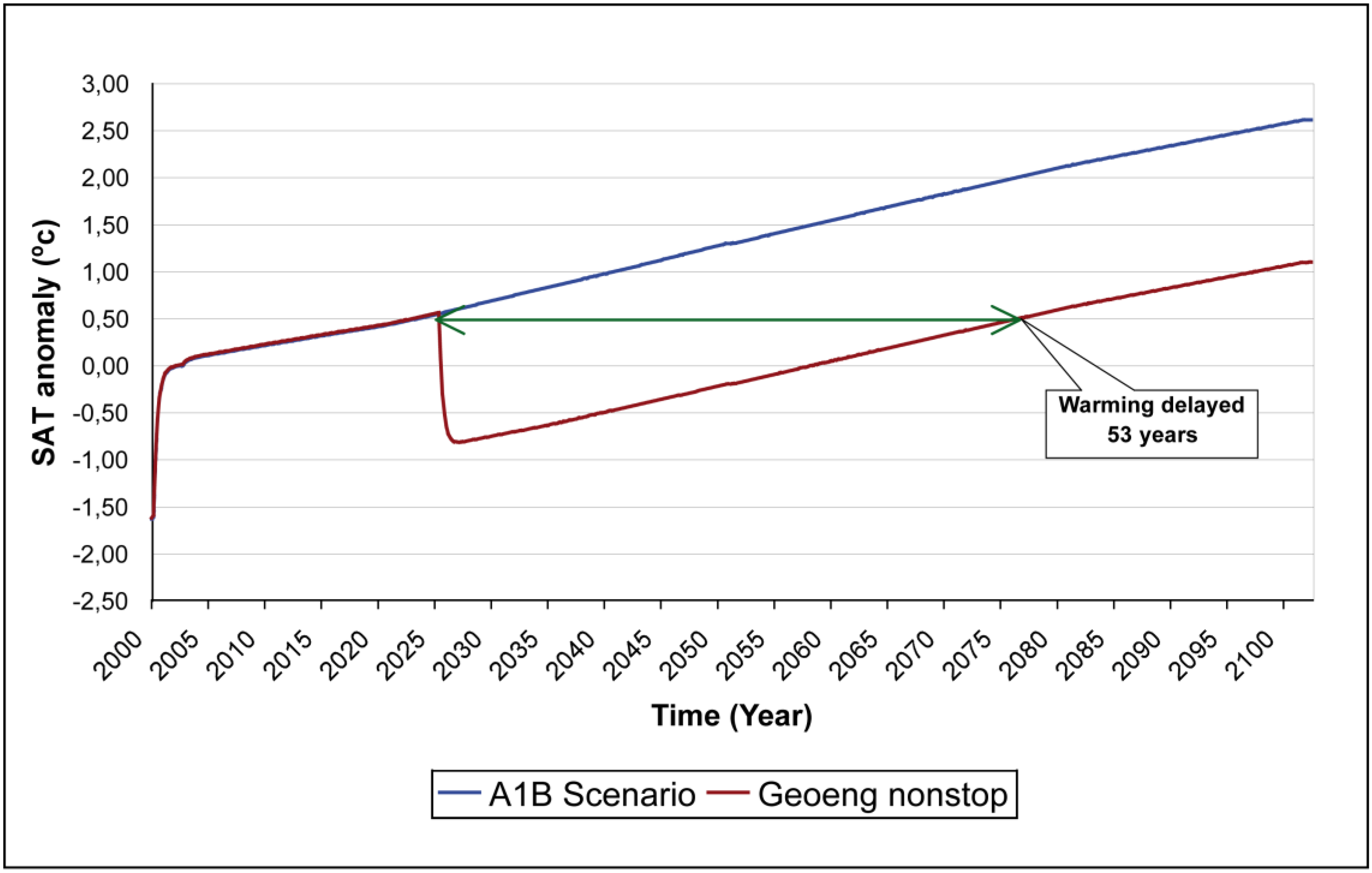
3.2. Geoengineering Deployment

In all the numerical experiments, sulphur injections into the stratosphere were set to start in 2025 and the injections were preset to take place every year thereafter. This frequency was selected in order to avoid the inter-annual temperature oscillations (due to changes in the aerosol loading) found by Wigley [14] when using lower frequencies of injections. The parameter a from Equation 1 was adjusted to account for the loading injected.

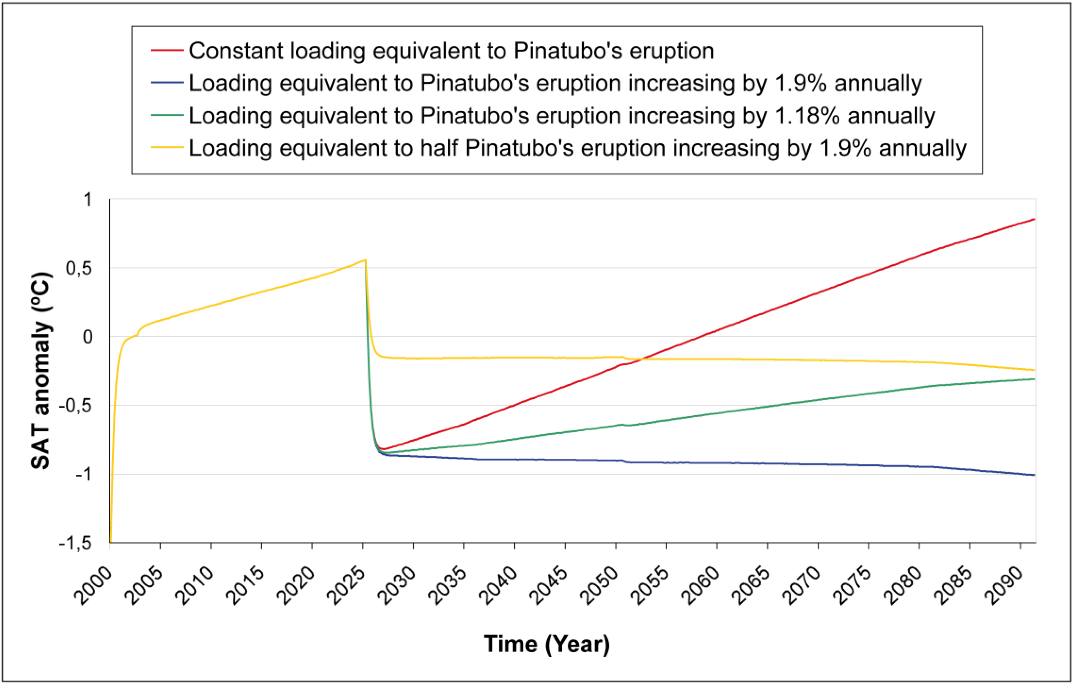
3.2.1. Loading equivalent to Pinatubo’s eruption kept constant through injections

The Pinatubo’s eruption injected about 10 TgS into the stratosphere [30] and, after 6 months, the remaining aerosol in the stratosphere that cooled the climate was about 6 TgS [13]. This means that, to produce a lasting cooling effect, a stratospheric loading of about 6 TgS should be maintained via man-made injections.
To simulate this case, it was assumed that the radiative forcing due to 6 TgS placed in the stratosphere was equivalent to assign parameter a (from the time-dependent albedo at the TOA formula) the value of 0.013. This assumption is supported by the successful simulation of Pinatubo’s eruption completed before. Moreover, to account for the constant aerosol loading, the albedo at the TOA was set to be constant from when the injections started.
In the first two years after the initial injection, the climate was rapidly cooled to preindustrial values. In fact, the largest temperature anomaly found, relative to the period 1980–1999 simulated in the OGIM, was −0.8 ºC. According to Jones et al. [42] this would fit with the expected values of the 17th century, the coldest century of the millennium. They stated that the 17th century would have been 0.5–0.8 ºC below the 1961–1990 average. Note that in this study, the reference period is 1980–1999 and, consequently, the temperature anomaly of the 17th century should be slightly higher relative to the period 1980–1999.
From the year 2027 onwards, the warming effect induced by increasing GHGs prevails over the cooling due to the aerosol shield and temperatures start to increase steadily unlike in the study made by Govindasamy and Caldeira [11] who kept the CO2 constant in the atmosphere after doubling.
Figure 1 shows that sulphur injections delayed the global warming by 53 years. This is in good agreement with Robock et al. [19]. In fact, they found a delay in the warming estimated for the A1B scenario of approximately 23 years when injecting about half of the loading injected here (2.5 TgS). This result supports the view that an anthropogenic sulphate aerosol layer is able to compensate for the ongoing global warming and is in good concordance with recent studies [20,21,22,23].
As Wigley [14] stated, this delay could provide valuable extra time to reduce the dependency of the energy system from fossil fuels before serious climate change unfolds.
Figure 1. A1B scenario with a loading injected equivalent to Mount Pinatubo’s eruption.
Atmosphere 01 00062 g001

3.2.2. Loading equivalent to Pinatubo’s eruption increasing every year

In the previous section it was found that, in order to keep the mean SAT constant within a world of increasing GHG abundances, the geoengineering intensity should be increased accordingly. Robock et al. [19] did not consider the possibility of increasing steadily in time the loading injected. In Brovkin et al. [20] it is stated that sulphur loading for complete compensation of GHG warming should be increased from 6.2 TgS in 2100 to 12.7 TgS in 2300. Eliseev et al. [22,23] have recently pointed out that sulphur injections would need to be doubled from 2050 to 2100. In this work we calculated the rate at which the loading of sulphur injected every year should be increased in order to induce a smooth stabilisation of the SAT. Furthermore, we translate this rate into additional emissions of sulphur and extra cost to be faced every year. We illustrate here that this geoengineering scheme, apart from being a long-term commitment, is bound with rising costs each year.
Parameter a in equation 1 was made time-dependent in order to account for the increasing sulphur loading to be injected every year (Equations 3 and 4). The following scenarios were selected to illustrate the effects of increasing aerosol loadings in the SAT.
a)
The loading injected increases by 1.9 % every year:
In this case, the parameter a starts with Pinatubo’s value (0.013) and is incremented every year by 1.9 % (r = 0.019). This means that every year the injection would be 114 kilotonnes of sulphur larger than the previous year. It should be borne in mind that, as the loading injected increases, the costs of deployment rise accordingly. In 1992 the estimated cost of injecting 1 TgS into the stratosphere was calculated to be US $25 billion [13]. Therefore, the deployment of 6 TgS per year would cost US $150 billion annually (ignoring changes in currency value). Assuming linearity in the relationship between costs and loading deployed, increasing the initial loading by 1.9% would cost an additional US $2.85 billion every year.
In this scenario, after rapid initial cooling, SAT anomalies are held slightly below preindustrial values (Figure 2). It is remarkable that increasing the loading injected every year by 114 kilotonnes of sulphur offsets the warming due to increasing GHGs in the atmosphere and keeps the SAT approximately constant.
Figure 2. Comparison of different geoengineering intensities within the A1B scenario.
Atmosphere 01 00062 g002
These results fit well with recent works carried out by Matthews and Caldeira [15] within the A2 SRES scenario, Brovkin et al. [20] whose baseline scenario was slightly less intensive in CO2 emissions than the A2, and Eliseev et al. [22,23] within the SRES A1B scenario. Matthews and Caldeira [15] used a geoengineering parameter that was preset to regulate the amount of solar radiation reaching the TOA to compensate for CO2 forcing. Similarly, in Eliseev et al. [22,23] emissions are set proportional to the TOA instantaneous radiative forcing imposed by CO2, CH4 and N2O. Brovkin et al. [20] preconditioned the amount of sulphur emissions in order to prevent exceeding a target temperature but they only took into account the forcing of CO2.
In our study the increase in geoengineering intensity was not automatically preset to match the increasing GHGs radiative forcing at the TOA or to prevent surpassing a predetermined SAT value. Therefore, we have experimentally calculated the increase of sulphate aerosol loading needed to keep SAT values constant. None of the previous studies explicitly calculated the rate of increase needed nor did they take into account the radiative forcing due to changing atmospheric abundances of CH4, N2O, O3 and CFCs altogether within the A1B scenario.
b)
The loading injected increases by 1.18 % every year:
As in the previous case, the parameter a starts with the Pinatubo’s value but here it is incremented by 1.18 % (r = 0.0118) on a yearly basis. In this case, the loading injected is increased every year by 70.8 kilotonnes of sulphur. This scheme would be cheaper to deploy, in fact, it would cost an additional US $1.77 billion every year.
As expected, the SAT quickly decreased to preindustrial values at the beginning of the injections. However, this geoengineering rate was found to be insufficient to counteract the warming effects due to increasing GHGs and, consequently, the SAT rose steadily since the initial cooling is achieved. Figure 2 shows that, at the end of the run (2,100), the mean SAT reached typical values of the 1970s or in other words, a SAT anomaly of ~(−0.3) ºC relative to the period 1980–1999 [43].

3.2.3. Loading equivalent to half of the amount injected by Pinatubo’s eruption increasing by 1.9% every year

In the previous cases, the initial cooling found once the injections started might be considered too large. In order, to reduce the magnitude of the initial SAT decrease, an extra case in which the initial aerosol loading is halved was analysed.
In this case, the parameter a was adjusted to start with a value of 0.0065 (assumed to be equivalent to deploying 3 TgS into the stratosphere) and preset to be increased every year by 1.9% (r = 0.019). Therefore, the loading injected increases by 57 kilotonnes of sulphur every year. As expected, the initial cooling was found to be more gradual and similar to the global average SAT decrease found by Robock et al. [19] when injecting a loading equivalent to 2.5 TgS.
The model needs three years (2000–2003) for spin-up. In this case, a SAT anomaly of ~ (−0.3) ºC relative to the baseline period 1980–1999 [43] was found. This means that the SAT was initially cooled to the 1970s values. From that point, the SAT was held approximately constant throughout all of the run length (Figure 2).

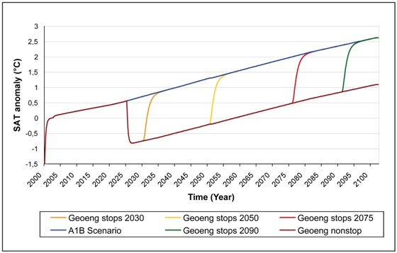
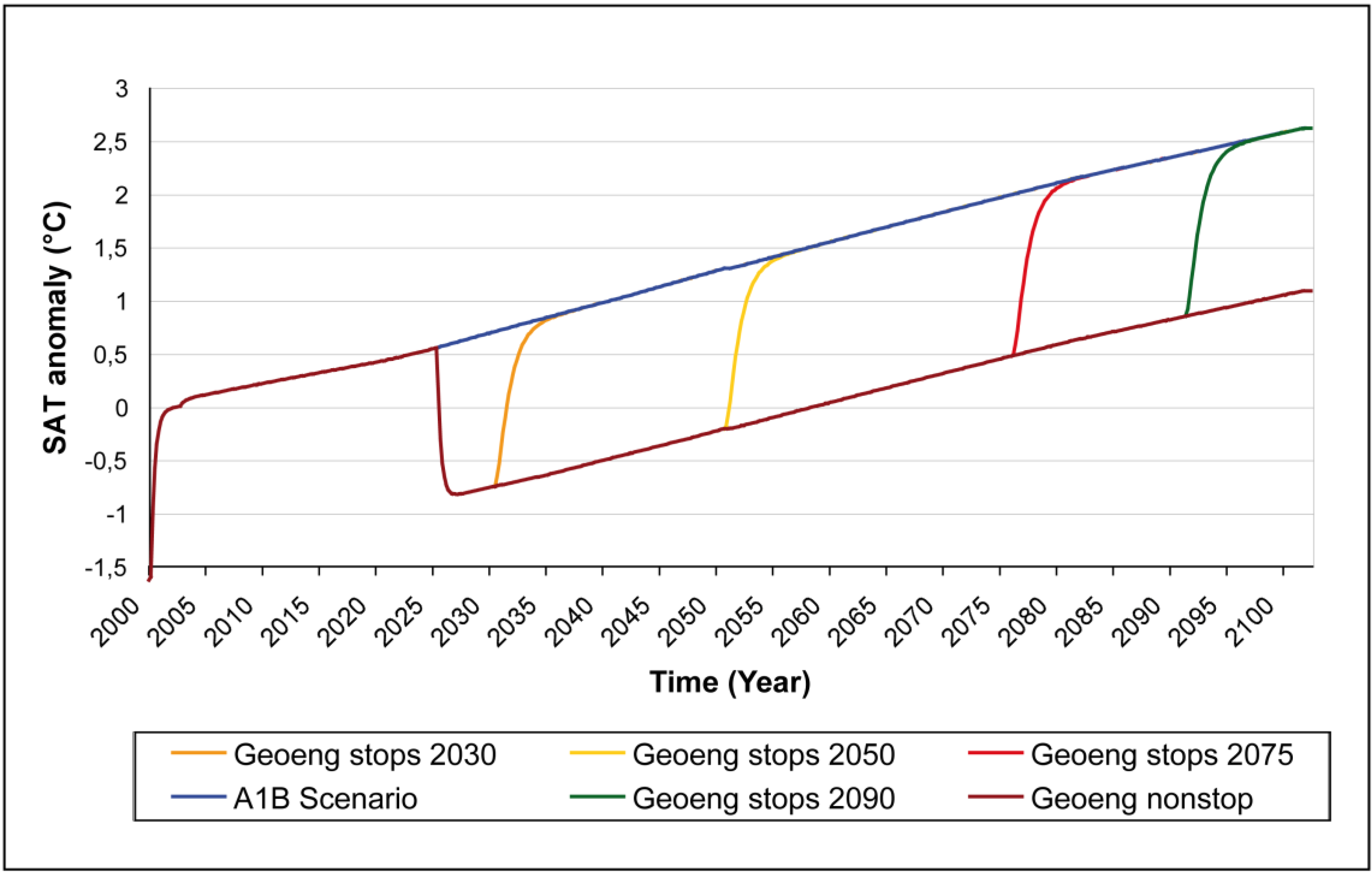
3.3. Geoengineering Failure Scenarios

As mentioned above, the continuous injection of sulphur into the stratosphere is associated with increasing costs and, in order to work, it would also require international agreement and stability in the long-term. This seems to be a fairly complicated scenario as any international conflict or technological failure might arise forcing an abrupt interruption of sulphur injections (geoengineering failure). In this section we therefore examine what would be the impact of an abrupt cessation of geoengineering at different dates and with different aerosol loadings. We assumed that the sulphate aerosol loading decreases exponentially with time once the failure takes place.

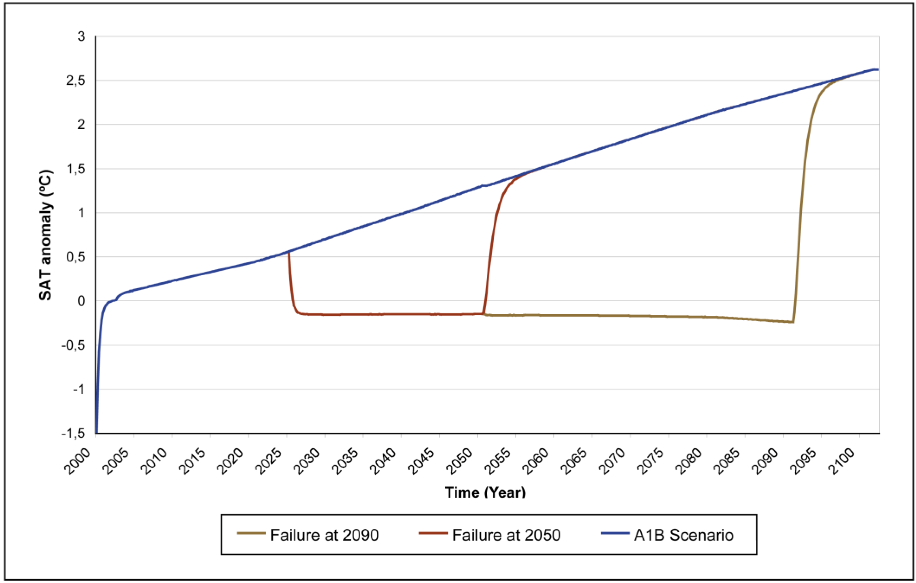
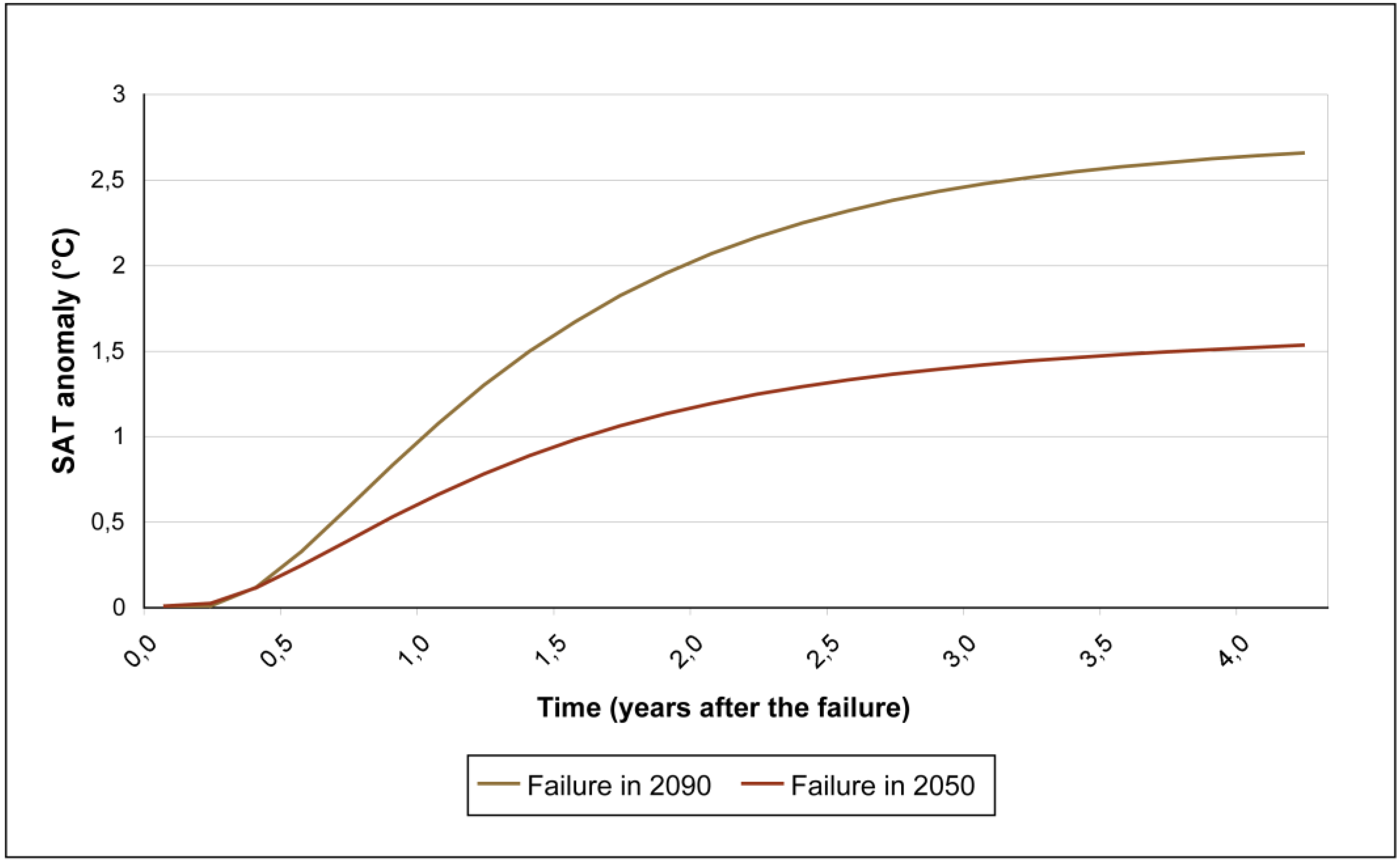
3.3.1. Injections interrupted at 2030, 2050, 2075 and 2090 with a constant aerosol loading

Figure 3 shows that, once the initial cooling is reached, if the negative radiative forcing exerted by the sulphate layer is kept constant in time, the positive radiative forcing exerted by increasing GHGs (according to A1B scenario) will eventually induce an increase in SAT. Note that, once the cooling effects of the sulphate layer have been overcome, the increasing rate of SAT is the same as in the ‘non-geoengineered scenario’ (A1B). We found that, in this scenario, the abrupt warming rate triggered after the geoengineering interruption is independent of when the failure takes place.
Figure 3. SAT response to geoengineering failures at different times with a constant loading equivalent to Mount Pinatubo’s eruption.
Atmosphere 01 00062 g003
The mean annual warming rate found in the first five years after the failure was 0.3 °C/year. It must be highlighted that this warming rate is 15 times larger than the current warming rate (0.02 °C/year) of the climate [15] and almost 43 times larger than the rate of annual warming for land areas observed in the twentieth century, which was 0.07 °C per decade according to Jones and Moberg [44].

3.3.2. Injections interrupted at 2050 and 2090 with a loading equivalent to half of the Pinatubo’s eruption increasing by 1.9% every year

This case was selected to illustrate the following point. It was found that, if the aerosol loading increases in time at an appropriate rate to (at least) compensate for the warming due to increasing GHGs, the later the geoengineering failure occurs, the larger the peak annual warming rate of SAT.
Figure 4 and Figure 5 show that, for the same loading initially injected, the warming rate with a failure after 75 years of injections will be considerably higher than after 25 years. In fact, it was found that the mean annual warming rate for the next five years with a failure at 2090 (0.56 °C/year) was 18% higher than the peak warming rate with a failure at 2050 (0.3 °C/year). In other words, the climate would warm 28 times faster than the current climate with the failure at 2090 and 15 times faster if the failure occurred at 2050.
Figure 4. SAT response to geoengineering failures at 2050 and 2090 with a constant loading equivalent to half of the Mount Pinatubo’s eruption.
Atmosphere 01 00062 g004
Figure 5. Globally averaged SAT warming after geoengineering failures at 2050 and 2090 with a constant loading equivalent to half of the Mount Pinatubo’s eruption.
Atmosphere 01 00062 g005

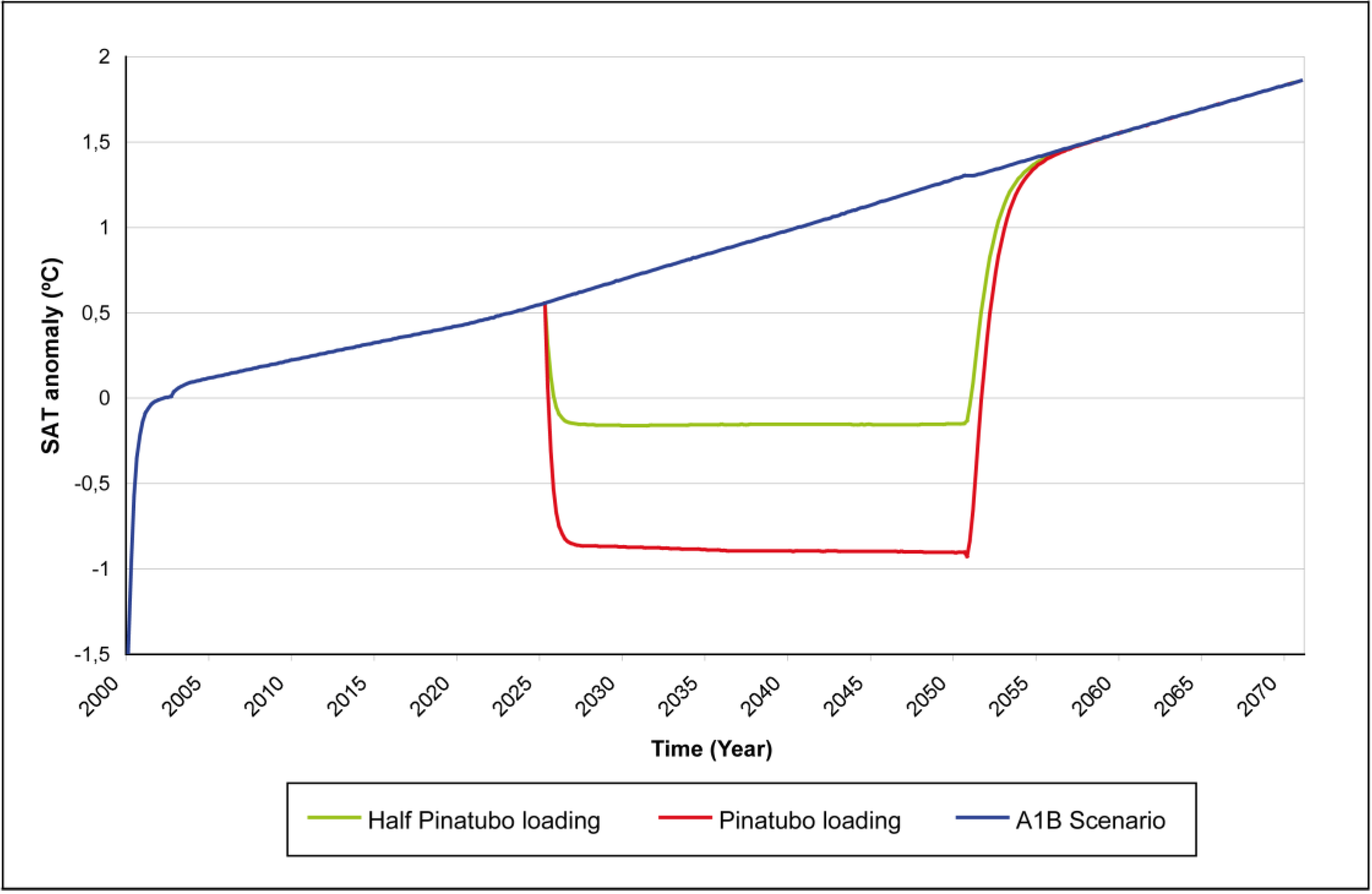
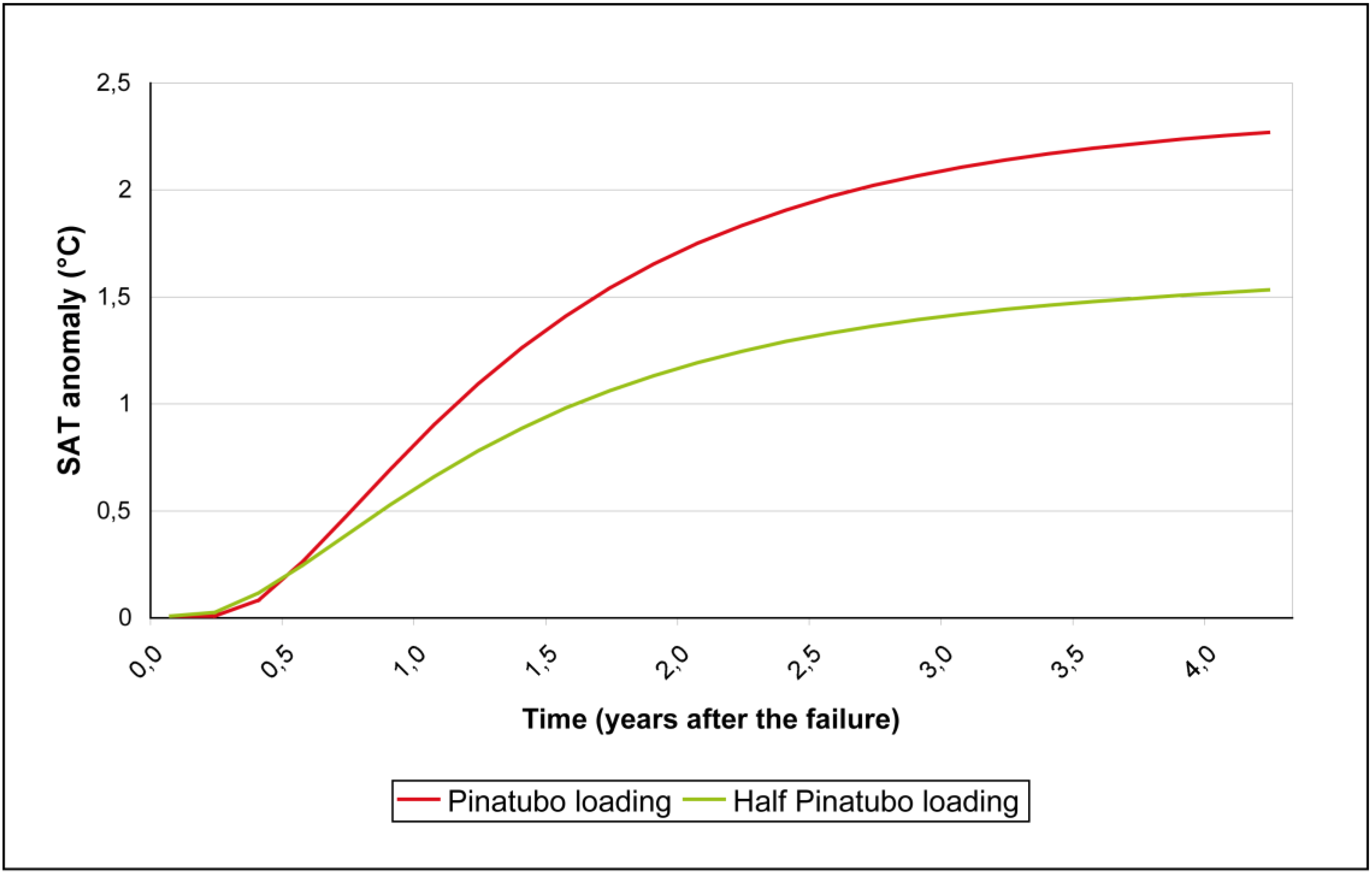
3.3.3. Injections interrupted at 2050 with different aerosol loadings

This case has been drawn to illustrate the point that, in case of a geoengineering failure, the warming rate of SAT to expect will be larger the higher the aerosol loading deployed in the stratosphere.
In this case, the first scenario was assigned a loading equivalent to that of Mount Pinatubo’s eruption (6 TgS) and the second one half of that loading. Both scenarios were preset to increase their respective loadings by 1.9 % every year.
It was found that the mean annual warming rate in the high loading scenario (0.46 ºC/year) was 15% larger than that of the low loading scenario (0.3 ºC/year) (see Figure 6 and Figure 7). In comparison with the current warming rate of climate according to Matthews and Caldeira [15], the abrupt warming triggered in the high loading scenario was found to be 20 times higher and 15 times in the low loading scenario.
Another finding was that the time needed for the cooling effects to be fully appreciated was 22 months after the first injection, independent of the loading injected.
The magnitude of the mean annual warming rates found seems to be reasonable and in line with recent studies which have examined this issue in different scenarios or from different perspectives [15,20,21,22,23].
Figure 6. SAT response to a geoengineering failure at 2050 with different aerosol loadings.
Atmosphere 01 00062 g006
Figure 7. Globally averaged SAT warming after a geoengineering failure at 2050 with different aerosol loadings.
Atmosphere 01 00062 g007

3.4. Shortcomings of This Geoengineering Scheme

Sulphur injections into the stratosphere present important caveats and side effects that must be thoroughly researched and evaluated in order to provide a sound assessment of this type of geoengineering before any other consideration is taken.
First of all and as shown in this study, an abrupt cessation of sulphur injections would unleash an unprecedented and catastrophic warming of the Earth. In addition to the climatic disruption, the world economy would be seriously damaged [45]. In order to prevent this situation, sulphur should be injected on a regular basis and for a long-term into the stratosphere.
Secondly, the questionable governance of these schemes must be highlighted. It seems unlikely that an international body specifically created for this purpose would be able to regulate the sulphur deployment and provide the stability required in the long-term [46].
Far from resolving the problem related with the ocean acidification [14,37,47], this technique might have secondary effects on pH and aragonite saturation [48]. In fact, the effect of lower temperatures in a geoengineered world with higher CO2 abundances would increase the CO2 solubility in the ocean [15] and alter the behaviour of terrestrial carbon sinks as well [48]. However, sulphur injections could delay sea-level rise by 40–80 years [49].
On the other hand, adding sulphur to the stratosphere might disrupt the hydrological cycle as highlighted by Trenberth and Dai [36]. They found an important decrease in precipitation over land after Mount Pinatubo eruption. Moreover, several modelling studies have found a reduction in global precipitation when simulating a geoengineered scenario [15,19,47,50]. In addition, as pointed out by Robock et al. [19], this geoengineering scheme might weaken the African and Asian summer monsoon causing widespread droughts and hunger.
Rasch et al. [50] noted that injecting sulphur into the stratosphere would moderately increase acid rain. However, they pointed out that this moderate increment might be offset by a reduction in tropospheric sulphur pollution.
Another shortcoming is that, even if the global mean SAT is kept constant by means of a uniformly distributed sulphate aerosol layer, there will always be temperature changes at the regional scale. Whether due to the patchy nature of the GHG forcing itself [51,52,53] or due to the aerosol lowering the albedo of land with high reflective surfaces [20]. This fact highlights the limitations of using the global mean SAT as an indicator of the climatic system and the need to define a set of more sophisticated anthropogenic climate-forcing indicators [46].
So even if we could keep the Earth’s temperature at roughly the same globally averaged SAT, it seems unlikely that all aspects of the physical system will behave in the same way as before human-induced GHG increases [50]. Furthermore, regional SAT anomalies expected in a geoengineered world could lead to regional conflict [37].
The deployment of an anthropogenic sulphate aerosol would induce a heating of the lower tropical stratosphere [7]. This would increase the stratospheric water vapour content enhancing catalytic ozone destruction cycles [54]. The warming of the tropical stratosphere would also promote polar ozone depletion as the temperature gradient between tropics and polar regions would increase and the polar vortex could be reinforced [55]. A larger temperature gradient would induce stronger westerlies and a winter warming over northern Eurasia and North America [56].
The reduction in ultra-violet solar radiation reaching the ground might also impact stratospheric but especially tropospheric chemistry [50]. On the other hand, the increase in diffuse radiation might enhance photosynthesis [57]. Robock [37] noted more shortcomings as the risk of military use of this technology, the reduction of incoming radiation for solar power systems, the whitening of the sky or the seeding of cirrus clouds.
Finally, the practical implementation of this geoengineering scheme seems to be a delicate and long commitment task [50]. Whether mixing sulphur into the fuel of commercial planes or firing large naval rifles or suspending hoses from stratospheric balloons, the implementation would be bound with environmental impact [58]. Izrael et al. [59] have recently accomplished field experiments in which they generated an artificial sulphate aerosol layer in the middle troposphere. They measured a temporal 1 % solar radiation reduction before the aerosol layer dissipated.

4. Conclusions

Our results show that the sulphur injections rapidly reduced the mean SAT of the Earth. In fact, with a constant loading equivalent to that injected in Mount Pinatubo’s eruption, SAT readily decreased to preindustrial values whereas when halving the aerosol loading, SAT values approached those of the 1970s. As expected, the magnitude of the initial cooling was dependent on the sulphur loading initially injected.
The cooling effect due to the sulphate aerosol layer begins shortly after the injections started in all the cases examined. This means that the deployment of this kind of geoengineering scheme could be postponed until dangerous climate change is at hand.
We found that, if an aerosol loading equivalent to 6 TgS was retained constant in time, the global warming would be delayed by 53 years. In this case, the global warming problem was not solved but displaced in time. However, this extra time could be valuable to fully implement the cut backs on GHG emissions. Nevertheless, provided that technology can ‘fix’ the problem, emission targets might be abandoned [60] with the GHG emissions surpassing the A1B SRES scenario estimates and, consequently, increasing the risk of larger warming rates in case of a geoengineering failure. It must be borne in mind that, once geoengineering is started, the commitment might be for several hundred years or, in other words, until the CO2 in excess is removed from the atmosphere [61].
Keeping the SAT constant in the context of increasing GHGs implies increasing the aerosol loading steadily with time. Within the A1B scenario context, it was found that an annual loading increase by 1.9 % counterbalanced the warming induced by increasing GHGs, independently of the aerosol loading initially injected. Therefore, the costs of keeping the SAT constant are expected to increase steadily in time.
Among all the cases examined, it was judged that deploying a loading equivalent to 3 TgS (half Pinatubo’s loading) and increasing it every year by 1.9% would be the least climatic disruptive option.
The analysis of different geoengineering failure scenarios confirmed that the maximum annual warming rate unleashed in the aftermath of a failure would be remarkably higher than the current warming rate of the climate. This could have dramatic effects for life on Earth as the capacity to adapt to such an abrupt global warming is limited.
Our results show that larger initial loadings induce more intense warming rates after a geoengineering failure. On the other hand, the warming rate was found to be independent of the timing of the failure on the condition that the aerosol loading had been kept constant until the injections were interrupted. Conversely, when the loading injected had been steadily increased with time, the later the injections were stopped the higher the warming rate found (on the condition that the loading injected is increased by at least 1.9% every year).
The work accomplished here, despite using a simple climate model, provides a new approach to this issue and fits reasonably well with recent studies [15,20,22,23]. The results obtained with this study should contribute to the growing body of evidence about the effects and risks of this geoengineering scheme.
Injecting sulphur into the stratosphere has theoretically proved to compensate for the increasing GHG forcing and, as Schneider [46] pointed out, the climatic disruptions that might unfold in a geoengineered scenario would not necessarily be worse than an unabated 5 ºC warming before 2100. Nonetheless, considering all the caveats and shortcomings and the uncertainties that remain, this geoengineering proposal should be regarded with extreme caution. Comprehensive scientific evaluation should be accomplished and many uncertainties must be clarified before we can even consider this scheme as a complement to emission cut backs.

Acknowledgements

We are thankful to R.M. MacKay and M.A.K. Khalil for making their climate model freely available and anonymous reviewers for helpful comments on the manuscript.

References

  1. Lenton, T.M.; Vaughan, N.E. The radiative forcing potential of different climate geoengineering options. Atmos. Chem. Phys. 2009, 9, 5539–5561. [Google Scholar] [CrossRef]
  2. Keith, D.W. Geoengineering. In Encyclopedia of Global Change; Oxford University Press: New York, NY, USA, 2002; pp. 495–502. [Google Scholar]
  3. Cotton, W.R.; Pielke, R.A. Human Impacts on Weather and Climate; Cambridge University Press: Cambridge, UK, 2007. [Google Scholar]
  4. Budyko, M.I. Climatic Changes. In American Geophysical Society; American Geophysical Union: Washington, DC, USA, 1977; p. 244. [Google Scholar]
  5. Meixner, F.X.; Georgii, H.W.; Ockelmann, G.; Jäger, H.; Reiter, R. The arrival of the Mount St. Helens eruption cloud over Europe. Geophys. Res. Lett. 1981, 8, 163–166. [Google Scholar] [CrossRef]
  6. Jones, P.D.; Kelly, P.M. The effect of tropical explosive volcanic eruptions in surface air temperature. In Reprint from the Climatic Research Unit; University of East Anglia: Norwich, UK, 1996. [Google Scholar]
  7. Robock, A. Volcanic eruptions and climate. Rev. Geophys. 2000, 38, 191–219. [Google Scholar] [CrossRef]
  8. Panel on Policy Implications of Greenhouse Warming; National Academy of Sciences; National Academy of Engineering; Institute of Medicine. Policy Implications of Greenhouse Warming: Mitigation, Adaptation, and the Science Base; The National Academies Press: Washington, DC, USA, 1992. [Google Scholar]
  9. Keith, D.W. Geoengineering the climate: History and prospect. Annu. Rev. Energ. Environ. 2000, 25, 245–284. [Google Scholar] [CrossRef]
  10. Barker, T.; Bashmakov, I.; Alharthi, A.; Amann, M.; Cifuentes, L.; Drexhage, J.; Duan, M.; Edenhofer, O.; Flannery, B.; Grubb, M.; Hoogwijk, M.; Ibitoye, F.I.; Jepma, C.J.; Pizer, W.A.; Yamaji, K. Mitigation from a cross-sectoral perspective. In Climate Change 2007: Mitigation of Climate Change; Contribution of Working Group III to the Fourth Assessment Report of the Intergovernmental Panel on Climate Change; Metz, B., Davidson, O.R., Bosch, P.R., Dave, R., Meyer, L.A., Eds.; Cambridge University Press: Cambridge, UK and New York, NY, USA, 2007. [Google Scholar]
  11. Govindasamy, B.; Caldeira, K. Geoengineering earth’s radiation balance to mitigate CO2 induced climate change. Geophys. Res. Lett. 2000, 27, 2141–2144. [Google Scholar] [CrossRef]
  12. Govindasamy, B.; Caldeira, K.; Duffy, P.B. Geoengineering Earth's radiation balance to mitigate climate change from a quadrupling of CO2. Global Planet. Change 2003, 37, 157–168. [Google Scholar] [CrossRef]
  13. Crutzen, P. Albedo enhancement by stratospheric sulfur injections: A contribution to resolve a policy dilemma? Climatic Change 2006, 77, 211–220. [Google Scholar] [CrossRef]
  14. Wigley, T.M. A combined mitigation/geoengineering approach to climate stabilization. Science 2006, 314, 452–454. [Google Scholar] [CrossRef]
  15. Matthews, H.D.; Caldeira, K. Transient climate-carbon simulations of planetary geoengineering. Proc. Natl. Acad. Sci USA 2007, 104, 9949–9954. [Google Scholar] [CrossRef]
  16. Nakicenovic, N.; Alcamo, J.; Davis, G.; de Vries, B.; Fenhann, J.; Gaffin, S.; Gregory, K.; Grubler, A.; Yong Jung, T.; Kram, T.; Lebre, La Rovere, E.; Michaelis, L.; Mori, S.; Morita, T.; Pepper, W.; Pitcher, H.; Price, L.; Riahi, K.; Roehrl, A.; Rogner, H.H.; Sankovski, A.; Schlesinger, M.; Shukla, P.; Smith, S.; Swart, R.; van Rooijen, S.; Victor, N.; Dadi, Z. Special Report on Emissions Scenarios (Intergovernmental Panel on Climate Change); Cambridge University Press: Cambridge, UK and New York, NY, USA, 2000. [Google Scholar]
  17. Lane, L.; Caldeira, K.; Chatfield, R.; Langhoff, S. Workshop Report on Managing Solar Radiation; National Aeronautics and Space Administration (NASA); Ames Research Center: Moffett Field, CA, USA, 2007. [Google Scholar]
  18. Rasch, P.J.; Crutzen, P.J.; Coleman, D.B. Exploring the geoengineering of climate using stratospheric sulfate aerosols: The role of particle size. Geophys. Res. Lett. 2008, 35, L02809. [Google Scholar]
  19. Robock, A.; Oman, L.; Stenchikov, G.L. Regional climate responses to geoengineering with tropical and Arctic SO2 injections. J. Geophys. Res. 2008, 113, D16101. [Google Scholar] [CrossRef]
  20. Brovkin, V.; Petoukhov, V.; Claussen, M.; Bauer, E.; Archer, D.; Jaeger, C. Geoengineering climate by stratospheric sulfur injections: Earth system vulnerability to technological failure. Climatic Change 2009, 92, 243–259. [Google Scholar] [CrossRef]
  21. Ross, A.; Matthews, H.D. Climate engineering and the risk of rapid climate change. Environ. Res. Lett. 2009, 4, 045103. [Google Scholar] [CrossRef]
  22. Eliseev, A.; Mokhov, I.; Karpenko, A. Global warming mitigation by means of controlled aerosol emissions into the stratosphere: Global and regional peculiarities of temperature response as estimated in IAP RAS CM simulations. Atmos. Ocean. Opt. 2009, 22, 388–395. [Google Scholar] [CrossRef]
  23. Eliseev, A.; Chernokulsky, A.; Karpenko, A.; Mokhov, I. Global warming mitigation by sulphur loading in the stratosphere: dependence of required emissions on allowable residual warming rate. Theor. Appl. Climatol. 2010, 101, 67–81. [Google Scholar] [CrossRef]
  24. Llanillo, P.J. The Influence of Planetary Geoengineering on the Surface Air Temperature. MSc Dissertation, University of East Anglia, Norwich, UK, 2008. [Google Scholar]
  25. Ehhalt, D.; Prather, M.; Dentener, F.; Derwent, R.; Dlugokencky, E.; Holland, E.; Isaksen, I.; Katima, J.; Kirchhoff, V.; Matson, P.; Midgley, P.; Wang, M. SRES Tables. Appendix II. Climate Change 2001: The Scientific Basis. In Contribution of Working Group I to the Third Assessment Report of the Intergovernmental Panel on Climate Change; Cambridge University Press: Cambridge, UK and New York, NY, USA, 2001. [Google Scholar]
  26. Joos, F.; Prentice, I.C.; Sitch, S.; Meyer, R.; Hooss, G.; Plattner, G.-K.; Gerber, S.; Hasselmann, K. Global warming feedbacks on terrestrial carbon uptake under the Intergovernmental Panel on Climate Change (IPCC) Emission Scenarios. Global Biogeochem. Cycle. 2001, 15, 891–907. [Google Scholar] [CrossRef]
  27. Prentice, I.C.; Farquhar, G.D.; Fasham, M.J.R.; Goulden, M.L.; Heimann, M.; Jaramillo, V.J.; Kheshgi, H.S.; Le Quéré, C.; Scholes, R.J.; Wallace, D.W.R. The Carbon Cycle and Atmospheric Carbon Dioxide. Climate Change 2001: The Scientific Basis. In Contribution of Working Group I to the Third Assessment Report of the Intergovernmental Panel on Climate Change; Cambridge University Press: Cambridge, UK and New York, NY, USA, 2001. [Google Scholar]
  28. Ehhalt, D.; Prather, M.; Dentener, F.; Derwent, R.; Dlugokencky, E.; Holland, E.; Isaksen, I.; Katima, J.; Kirchhoff, V.; Matson, P.; Midgley, P.; Wang, M. Atmospheric Chemistry and Greenhouse Gases. Climate Change 2001: The Scientific Basis. In Contribution of Working Group I to the Third Assessment Report of the Intergovernmental Panel on Climate Change; Cambridge University Press: Cambridge, UK and New York, NY, USA, 2001. [Google Scholar]
  29. Kelly, P.M.; Jones, P.D.; Pengqun, J. The spatial response of the climate system to explosive volcanic eruptions. Int. J. Climatol. 1996, 16, 537–550. [Google Scholar] [CrossRef]
  30. Bluth, G.J.S.; Doiron, S.D.; Schnetzler, C.C.; Krueger, A.J.; Walter, L.S. Global tracking of the SO2 clouds from the June, 1991 Mount Pinatubo eruptions. Geophys. Res. Lett. 1992, 19, 151–154. [Google Scholar] [CrossRef]
  31. Hansen, J.; Lacis, A.; Ruedy, R.; Sato, M. Potential climate impact of Mount Pinatubo eruption. Geophys. Res. Lett. 1992, 19, 215–218. [Google Scholar] [CrossRef]
  32. Parker, D.E.; Wilson, H.; Jones, P.D.; Christy, J.R.; Folland, C.K. The impact of Mount Pinatubo on world-wide temperatures. Int. J. Climatol. 1996, 16, 487–497. [Google Scholar] [CrossRef]
  33. Jones, P.D.; Moberg, A.; Osborn, T.J.; Briffa, K.R. Surface climate responses to explosive volcanic eruptions seen in long European temperature records and mid-to-high latitude tree-ring density around the Northern Hemisphere. In Volcanism and the Earth’s Atmosphere; Robock, A., Oppenheimer, C., Eds.; American Geophysical Union: Washington, DC, USA, 2003; pp. 239–254. [Google Scholar]
  34. MacKay, R.M.; Khalil, M.A.K. Theory and development of a one dimensional time dependent radiative convective climate model. Chemosphere 1991, 22, 383–417. [Google Scholar] [CrossRef]
  35. Forest, C.E.; Stone, P.H.; Sokolov, A.P. Estimated PDFs of climate system properties including natural and anthropogenic forcings. Geophys. Res. Lett. 2006, 33, L01705. [Google Scholar]
  36. Trenberth, K.E.; Dai, A. Effects of mount pinatubo volcanic eruption on the hydrological cycle as an analog of geoengineering. Geophys. Res. Lett. 2007, 34, L15702. [Google Scholar] [CrossRef]
  37. Robock, A. Twenty reasons why geoengineering might be a bad idea. Bull. Atom. Sci. 2008, 64, 14–18. [Google Scholar] [CrossRef]
  38. U.S. Standard Atmosphere; National Oceanic and Atmospheric Administration (NOAA) and National Aeronautics and Space Administration (NASA): Washington, DC, USA, 1976.
  39. Meehl, G.A.; Stocker, T.F.; Collins, W.D.; Friedlingstein, P.; Gaye, A.T.; Gregory, J.M.; Kitoh, A.; Knutti, R.; Murphy, J.M.; Noda, A.; Raper, S.C.B; Watterson, I.J.; Weaver, A.J.; Zhao, Z.C. Global Climate Projections. In Climate Change 2007: The Physical Science Basis; Contribution of Working Group I to the Fourth Assessment Report of the Intergovernmental Panel on Climate Change; Cambridge University Press: Cambridge, UK and New York, NY, USA, 2007. [Google Scholar]
  40. Decker, R.; Decker, B. Volcanoes; Freeman: New York, NY, USA, 1997. [Google Scholar]
  41. Martí, J.; Ernst, G. Volcanoes and the Environment; Cambridge University Press: Cambridge, UK, 2005. [Google Scholar]
  42. Jones, P.D.; New, M.; Parker, D.E.; Martin, S.; Rigor, I.G. Surface air temperature and its changes over the past 150 years. Rev. Geophys. 1999, 37, 173–199. [Google Scholar] [CrossRef]
  43. Trenberth, K.E.; Jones, P.D.; Ambenje, P.; Bojariu, R.; Easterling, D.; Klein Tank, A.; Parker, D.; Rahimzadeh, F.; Renwick, J.A.; Rusticucci, M.; Soden, B.; Zhai, P. Observations: Surface and Atmospheric Climate Change. In Climate Change 2007: The Physical Science Basis; Contribution of Working Group I to the Fourth Assessment Report of the Intergovernmental Panel on Climate Change; Cambridge University Press: Cambridge, UK and New York, NY, USA, 2007. [Google Scholar]
  44. Jones, P.D.; Moberg, A. Hemispheric and large-scale surface air temperature variations: An extensive revision and an update to 2001. J. Clim. 2003, 16, 206–223. [Google Scholar] [CrossRef]
  45. Goes, M.; Tuana, N.; Keller, K. The Economics (or lack thereof) of Aerosol Geoengineering. Climatic Change 2010. in review. [Google Scholar]
  46. Schneider, S.H. Geoengineering: Could— or should— we do it? Climatic Change 1996, 33, 291–302. [Google Scholar] [CrossRef]
  47. Bala, G.; Duffy, P.B.; Taylor, K.E. Impact of geoengineering schemes on the global hydrological cycle. Proc. Natl. Acad. Sci USA 2008, 105, 7664–7669. [Google Scholar] [CrossRef]
  48. Matthews, H.D.; Cao, L.; Caldeira, K. Sensitivity of ocean acidification to geoengineered climate stabilization. Geophys. Res. Lett. 2009, 36, L10706. [Google Scholar] [CrossRef]
  49. Moore, J.C.; Jevrejeva, S.; Grinsted, A. Efficacy of geoengineering to limit 21st century sea-level rise. Proc. Natl. Acad. Sci USA 2010, 107, 15699–15703. [Google Scholar] [CrossRef] [Green Version]
  50. Rasch, P.J.; Tilmes, S.; Turco, R.P.; Robock, A.; Oman, L.; Chen, C.C.; Stenchikov, G.L.; Garcia, R.R. An overview of geoengineering of climate using stratospheric sulphate aerosols. Phil. Trans. Roy. Soc. A—Math. Phy. 2008, 366, 4007–4037. [Google Scholar] [CrossRef]
  51. Schneider, S.H. Detecting Climatic Change Signals: Are There Any “Fingerprints”? Science 1994, 263, 341–347. [Google Scholar]
  52. Schneider, S.H. Earth systems engineering and management. Nature 2001, 409, 417–421. [Google Scholar] [CrossRef]
  53. Schneider, S.H. Geoengineering: could we or should we make it work? Phil. Trans. Roy. Soc. A—Math. Phy. 2008, 366, 3843–3862. [Google Scholar] [CrossRef]
  54. Kenzelmann, P.; Peter, T.; Fueglistaler, S.; Weisenstein, D.; Luo, D.; Schraner, M.; Rozanov, E. Geo-engineering side effects: Heating the tropical tropopause by sedimenting sulphur aerosol? In IOP Conference Series: Earth and Environmental Science; Institute for Atmospheric and Climate Science, ETH Zurich: Zürich, Switzerland, 2009; Volume 6, p. 452017. [Google Scholar]
  55. Tilmes, S.; Muller, R.; Salawitch, R. The sensitivity of polar ozone depletion to proposed geoengineering schemes. Science 2008, 320, 1201–1204. [Google Scholar] [CrossRef]
  56. Stenchikov, G.; Hamilton, K.; Stouffer, R.J.; Robock, A.; Ramaswamy, V.; Santer, B.; Graf, H.-F. Arctic Oscillation response to volcanic eruptions in the IPCC AR4 climate models. J. Geophys. Res. 2006, 111, D07107. [Google Scholar]
  57. Gu, L.; Baldocchi, D.D.; Wofsy, S.C.; Munger, J.W.; Michalsky, J.J.; Urbanski, S.P.; Boden, T.A. Response of a deciduous forest to the mount Pinatubo eruption: Enhanced photosynthesis. Science 2003, 299, 2035–2038. [Google Scholar] [CrossRef]
  58. Robock, A. Atmospheric science. Whither geoengineering? Science 2008, 320, 1166–1167. [Google Scholar] [CrossRef]
  59. Izrael, Y.; Zakharov, V.; Petrov, N.; Ryaboshapko, A.; Ivanov, V.; Savchenko, A.; Andreev, Y.; Eran’kov, V.; Puzov, Y.; Danilyan, B.; Kulyapin, V.; Gulevskii, V. Field studies of a geo-engineering method of maintaining a modern climate with aerosol particles. Russ. Meteorol. Hydrol. 2009, 34, 635–638. [Google Scholar] [CrossRef]
  60. Brewer, P.G. Evaluating a technological fix for climate. Proc. Nat. Acad. Sci. USA 2007, 104, 9915–9916. [Google Scholar] [CrossRef]
  61. Bengtsson, L. Geo-Engineering to Confine Climate Change: Is it at all feasible? Climatic Change 2006, 77, 229–234. [Google Scholar] [CrossRef]

