Assessment of Maximum Possible Urbanization Influences on Land Temperature Data by Comparison of Land and Marine Data around Coasts

Abstract
:1. Introduction
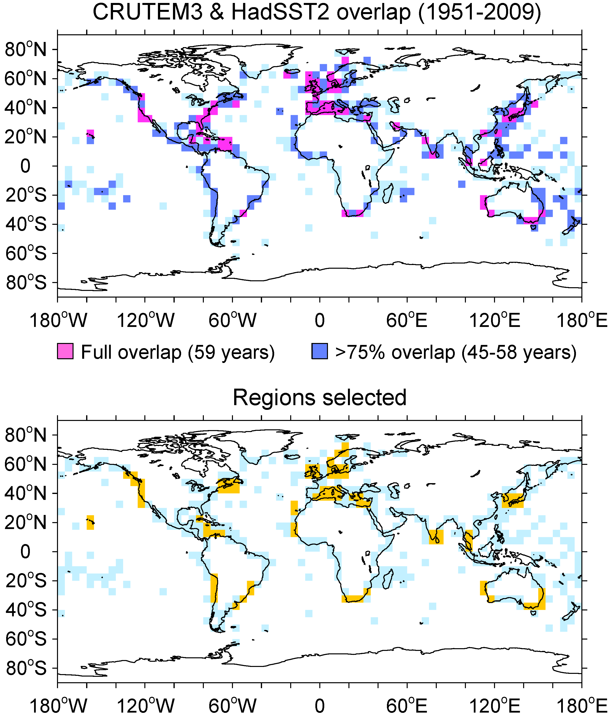
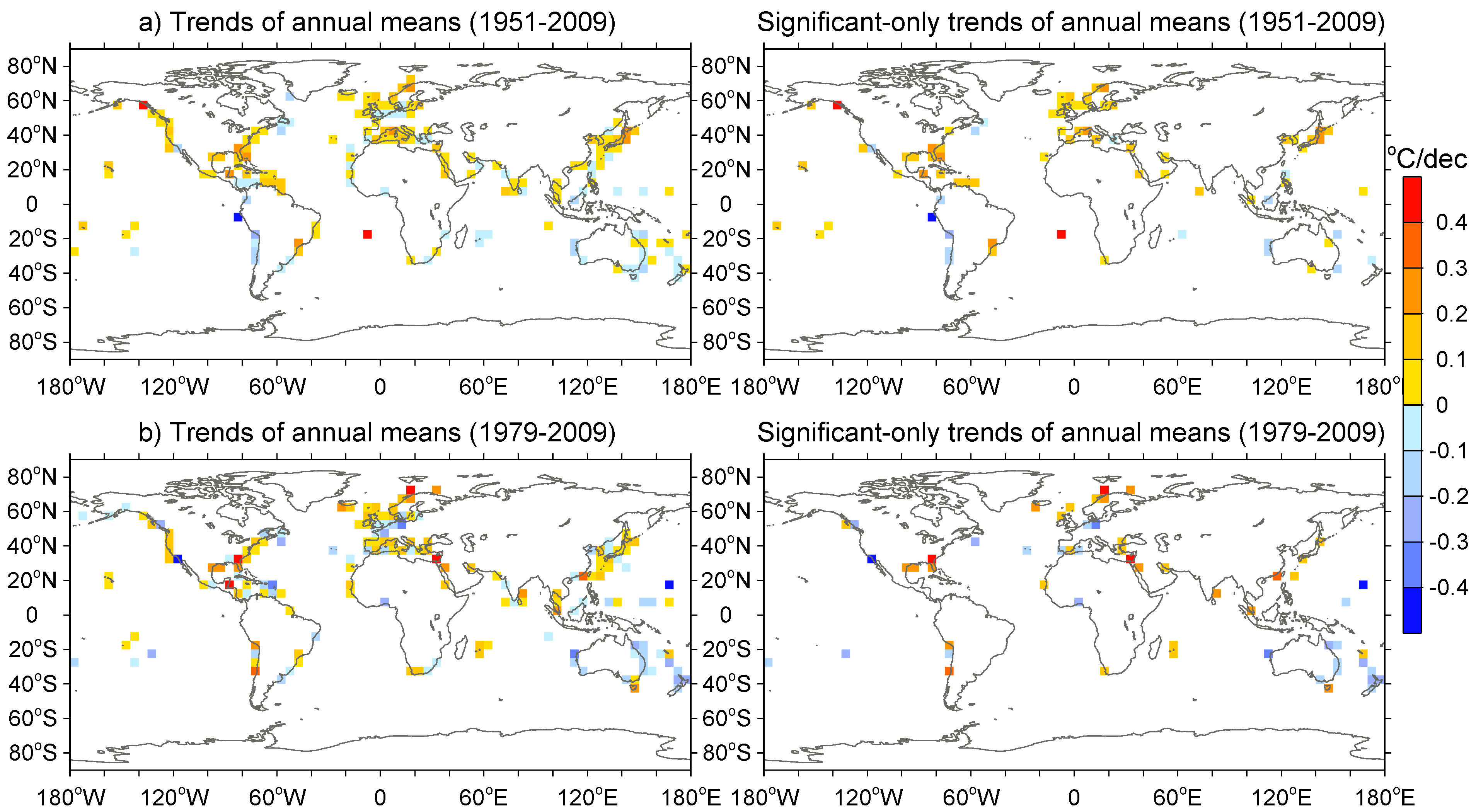
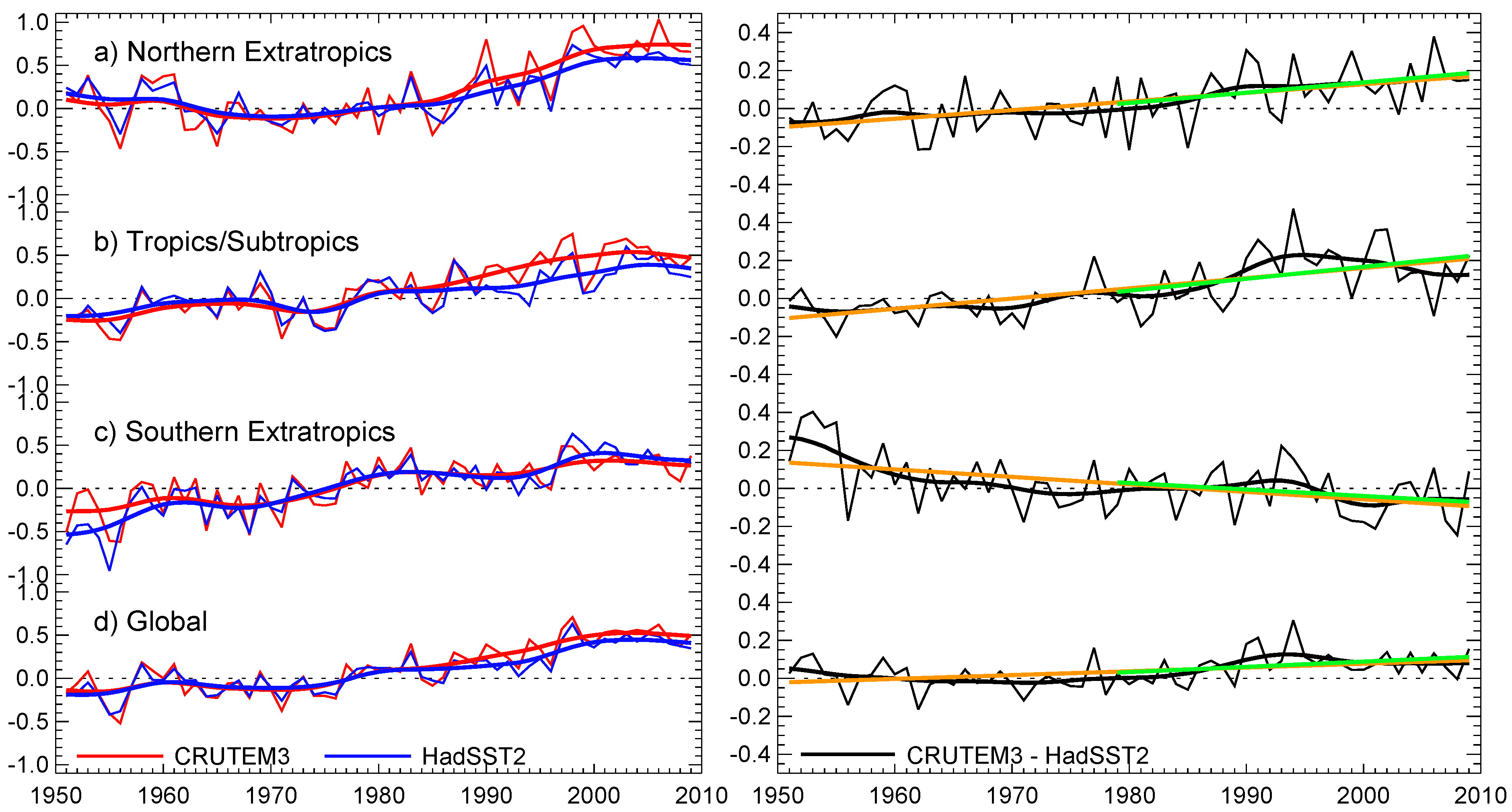
2. Data and Methods

| Region | 1951–2009 | 1951–1979 | 1979–2009 | ||||||||||||||
|---|---|---|---|---|---|---|---|---|---|---|---|---|---|---|---|---|---|
| ANN | DJF | MAM | JJA | SON | ANN | DJF | MAM | JJA | SON | ANN | DJF | MAM | JJA | SON | |||
| Northern Extratropics | |||||||||||||||||
| West Mediterranean (7) | 0.22 | 0.21 | 0.34 | 0.20 | 0.14 | −0.10 | −0.24 | −0.21 | −0.24 | 0.32 | 0.35 | 0.54 | 0.58 | 0.19 | 0.19 | ||
| 0.10 | 0.09 | 0.15 | 0.09 | 0.07 | −0.07 | −0.08 | −0.16 | −0.10 | 0.05 | 0.26 | 0.30 | 0.42 | 0.17 | 0.18 | |||
| 0.12 | 0.12 | 0.19 | 0.10 | 0.07 | −0.04 | −0.16 | −0.06 | −0.15 | 0.27 | 0.09 | 0.23 | 0.16 | 0.02 | 0.01 | |||
| East Mediterranean (4) | 0.10 | 0.12 | 0.21 | 0.08 | 0.01 | −0.12 | 0.11 | −0.27 | −0.25 | −0.12 | 0.48 | 0.48 | 0.70 | 0.39 | 0.43 | ||
| 0.07 | 0.03 | 0.12 | 0.09 | 0.06 | −0.11 | −0.04 | −0.10 | −0.22 | −0.10 | 0.32 | 0.25 | 0.39 | 0.38 | 0.35 | |||
| 0.03 | 0.09 | 0.10 | −0.01 | −0.05 | −0.02 | 0.15 | −0.17 | −0.03 | −0.02 | 0.16 | 0.23 | 0.30 | 0.01 | 0.08 | |||
| Britain–Ireland (4) | 0.17 | 0.17 | 0.17 | 0.13 | 0.18 | −0.03 | −0.21 | 0.04 | −0.04 | 0.08 | 0.44 | 0.49 | 0.31 | 0.45 | 0.32 | ||
| 0.13 | 0.13 | 0.15 | 0.13 | 0.10 | −0.02 | −0.04 | 0.03 | 0.03 | −0.06 | 0.39 | 0.41 | 0.36 | 0.42 | 0.34 | |||
| 0.04 | 0.03 | 0.02 | 0.00 | 0.09 | −0.01 | −0.16 | 0.01 | 0.01 | 0.15 | 0.06 | 0.09 | −0.05 | 0.03 | −0.02 | |||
| South Scandinavia (6) | 0.26 | 0.35 | 0.22 | 0.11 | 0.34 | 0.03 | 0.11 | 0.03 | −0.09 | 0.09 | 0.61 | 0.59 | 0.57 | 0.42 | 0.61 | ||
| 0.24 | 0.37 | 0.31 | 0.12 | 0.15 | 0.07 | 0.17 | 0.10 | −0.03 | −0.02 | 0.70 | 0.80 | 0.76 | 0.61 | 0.54 | |||
| 0.01 | −0.03 | −0.09 | −0.01 | 0.18 | −0.04 | −0.06 | −0.07 | −0.06 | 0.11 | −0.09 | −0.21 | −0.19 | −0.19 | 0.06 | |||
| Northeast Norway (4) | 0.23 | 0.25 | 0.18 | 0.11 | 0.37 | −0.12 | 0.06 | 0.05 | −0.44 | −0.17 | 0.60 | 0.34 | 0.48 | 0.56 | 0.86 | ||
| 0.05 | 0.05 | 0.11 | 0.02 | 0.03 | −0.06 | −0.03 | 0.10 | −0.24 | −0.14 | 0.34 | 0.33 | 0.38 | 0.30 | 0.36 | |||
| 0.18 | 0.21 | 0.07 | 0.08 | 0.34 | −0.06 | 0.08 | −0.05 | −0.20 | −0.03 | 0.26 | 0.02 | 0.10 | 0.26 | 0.50 | |||
| Korea–Japan (6) | 0.17 | 0.19 | 0.11 | 0.20 | 0.19 | 0.04 | 0.04 | 0.12 | 0.03 | −0.03 | 0.37 | 0.36 | 0.23 | 0.42 | 0.51 | ||
| 0.10 | 0.12 | 0.07 | 0.10 | 0.13 | −0.04 | −0.08 | 0.00 | 0.01 | −0.07 | 0.30 | 0.30 | 0.22 | 0.34 | 0.37 | |||
| 0.07 | 0.07 | 0.04 | 0.10 | 0.06 | 0.09 | 0.12 | 0.12 | 0.02 | 0.04 | 0.07 | 0.05 | 0.01 | 0.09 | 0.14 | |||
| West USA–Canada (7) | 0.12 | 0.18 | 0.15 | 0.04 | 0.11 | 0.00 | 0.01 | 0.11 | −0.06 | −0.07 | 0.01 | −0.08 | 0.13 | −0.02 | −0.13 | ||
| 0.05 | 0.11 | 0.09 | −0.03 | 0.02 | −0.12 | −0.07 | −0.07 | −0.16 | −0.19 | −0.08 | −0.09 | 0.01 | −0.17 | −0.12 | |||
| 0.07 | 0.07 | 0.05 | 0.08 | 0.10 | 0.11 | 0.08 | 0.17 | 0.09 | 0.11 | 0.09 | 0.01 | 0.12 | 0.15 | −0.01 | |||
| East USA–Canada (6) | 0.06 | 0.06 | 0.15 | 0.07 | −0.01 | −0.24 | −0.14 | 0.16 | −0.24 | −0.58 | 0.16 | −0.12 | 0.24 | 0.30 | 0.24 | ||
| 0.12 | 0.13 | 0.20 | 0.13 | 0.08 | −0.22 | −0.26 | −0.07 | −0.14 | −0.23 | 0.24 | 0.10 | 0.38 | 0.25 | 0.25 | |||
| −0.07 | −0.07 | −0.05 | −0.07 | −0.09 | −0.02 | 0.12 | 0.22 | −0.10 | −0.35 | −0.09 | −0.22 | −0.14 | 0.05 | −0.02 | |||
| AVERAGE | 0.15 | 0.17 | 0.17 | 0.11 | 0.13 | −0.07 | −0.03 | 0.04 | −0.14 | −0.12 | 0.30 | 0.23 | 0.34 | 0.30 | 0.30 | ||
| 0.10 | 0.12 | 0.14 | 0.08 | 0.08 | −0.10 | −0.09 | −0.04 | −0.11 | −0.12 | 0.25 | 0.23 | 0.31 | 0.23 | 0.24 | |||
| 0.05 | 0.05 | 0.04 | 0.04 | 0.06 | 0.03 | 0.05 | 0.07 | −0.03 | 0.00 | 0.05 | 0.01 | 0.03 | 0.07 | 0.07 | |||
| Tropics/Subtropics | |||||||||||||||||
| Northwest Africa (5) | 0.17 | 0.14 | 0.14 | 0.18 | 0.21 | −0.04 | −0.20 | −0.14 | −0.02 | 0.14 | 0.26 | 0.27 | 0.32 | 0.23 | 0.25 | ||
| 0.15 | 0.13 | 0.14 | 0.16 | 0.15 | −0.04 | −0.09 | −0.09 | −0.01 | 0.05 | 0.24 | 0.17 | 0.25 | 0.30 | 0.24 | |||
| 0.02 | 0.01 | 0.00 | 0.01 | 0.06 | −0.01 | −0.11 | −0.05 | 0.00 | 0.09 | 0.02 | 0.11 | 0.07 | −0.08 | 0.01 | |||
| South India (4) | 0.16 | 0.16 | 0.15 | 0.14 | 0.19 | 0.04 | 0.11 | 0.05 | 0.00 | 0.03 | 0.14 | 0.02 | 0.17 | 0.16 | 0.20 | ||
| 0.12 | 0.09 | 0.15 | 0.16 | 0.11 | 0.17 | 0.13 | 0.20 | 0.18 | 0.16 | 0.04 | −0.02 | 0.10 | 0.13 | 0.05 | |||
| 0.04 | 0.07 | −0.01 | −0.02 | 0.07 | −0.13 | −0.01 | −0.15 | −0.18 | −0.13 | 0.10 | 0.04 | 0.07 | 0.03 | 0.15 | |||
| Thailand (3) | 0.17 | 0.15 | 0.17 | 0.15 | 0.21 | 0.07 | 0.08 | 0.07 | 0.07 | 0.10 | 0.24 | 0.15 | 0.26 | 0.25 | 0.31 | ||
| 0.12 | 0.08 | 0.16 | 0.12 | 0.10 | 0.05 | −0.05 | 0.08 | 0.10 | 0.00 | 0.11 | 0.04 | 0.15 | 0.10 | 0.16 | |||
| 0.05 | 0.07 | 0.02 | 0.03 | 0.10 | 0.01 | 0.13 | −0.02 | −0.03 | 0.10 | 0.13 | 0.11 | 0.11 | 0.15 | 0.16 | |||
| Hawaii (2) | 0.15 | 0.14 | 0.19 | 0.16 | 0.11 | 0.36 | 0.40 | 0.33 | 0.37 | 0.30 | 0.01 | 0.01 | 0.07 | −0.04 | −0.05 | ||
| 0.04 | 0.03 | 0.04 | 0.05 | 0.03 | 0.04 | −0.02 | −0.01 | 0.07 | 0.06 | −0.03 | −0.03 | 0.03 | −0.05 | −0.08 | |||
| 0.11 | 0.11 | 0.14 | 0.11 | 0.08 | 0.33 | 0.41 | 0.34 | 0.31 | 0.24 | 0.04 | 0.04 | 0.04 | 0.01 | 0.02 | |||
| Caribbean (6) | 0.11 | 0.10 | 0.12 | 0.10 | 0.12 | −0.08 | −0.09 | −0.08 | −0.13 | −0.12 | 0.21 | 0.14 | 0.23 | 0.25 | 0.23 | ||
| 0.06 | 0.06 | 0.07 | 0.06 | 0.05 | −0.06 | −0.03 | −0.09 | −0.10 | −0.04 | 0.18 | 0.12 | 0.19 | 0.27 | 0.16 | |||
| 0.05 | 0.04 | 0.05 | 0.04 | 0.07 | −0.02 | −0.06 | 0.01 | −0.03 | −0.08 | 0.03 | 0.02 | 0.04 | −0.02 | 0.07 | |||
| AVERAGE | 0.15 | 0.14 | 0.15 | 0.15 | 0.17 | 0.07 | 0.06 | 0.04 | 0.06 | 0.09 | 0.17 | 0.12 | 0.21 | 0.17 | 0.19 | ||
| 0.10 | 0.08 | 0.11 | 0.11 | 0.09 | 0.03 | −0.01 | 0.02 | 0.05 | 0.05 | 0.11 | 0.05 | 0.14 | 0.15 | 0.11 | |||
| 0.05 | 0.06 | 0.04 | 0.03 | 0.08 | 0.04 | 0.07 | 0.03 | 0.01 | 0.04 | 0.06 | 0.06 | 0.07 | 0.02 | 0.08 | |||
| Southern Extratropics | |||||||||||||||||
| South Africa (4) | 0.19 | 0.20 | 0.18 | 0.18 | 0.17 | 0.17 | 0.20 | 0.10 | 0.12 | 0.18 | 0.15 | 0.07 | 0.17 | 0.20 | 0.14 | ||
| 0.15 | 0.16 | 0.13 | 0.14 | 0.14 | 0.21 | 0.29 | 0.09 | 0.14 | 0.29 | 0.08 | 0.00 | 0.09 | 0.17 | 0.03 | |||
| 0.04 | 0.04 | 0.05 | 0.04 | 0.02 | −0.04 | −0.09 | 0.01 | −0.02 | −0.11 | 0.06 | 0.07 | 0.08 | 0.03 | 0.11 | |||
| West Australia (3) | 0.06 | 0.11 | 0.10 | 0.06 | −0.05 | 0.25 | 0.15 | 0.30 | 0.15 | 0.36 | −0.09 | −0.02 | 0.00 | −0.16 | −0.18 | ||
| 0.16 | 0.22 | 0.22 | 0.13 | 0.08 | 0.25 | 0.20 | 0.33 | 0.24 | 0.22 | 0.11 | 0.20 | 0.12 | 0.04 | 0.09 | |||
| −0.11 | −0.11 | −0.13 | −0.07 | −0.13 | 0.00 | −0.05 | −0.04 | −0.09 | 0.14 | −0.21 | −0.22 | −0.12 | −0.20 | −0.27 | |||
| East Australia (5) | 0.13 | 0.09 | 0.12 | 0.17 | 0.16 | 0.13 | 0.09 | 0.08 | 0.11 | 0.26 | 0.06 | −0.08 | 0.13 | 0.15 | 0.09 | ||
| 0.18 | 0.15 | 0.19 | 0.20 | 0.19 | 0.29 | 0.33 | 0.29 | 0.25 | 0.29 | 0.18 | 0.08 | 0.20 | 0.23 | 0.24 | |||
| −0.05 | −0.06 | −0.07 | −0.03 | −0.03 | −0.16 | −0.24 | −0.21 | −0.14 | −0.03 | −0.12 | −0.16 | −0.06 | −0.09 | −0.15 | |||
| North Chile (4) | 0.00 | 0.02 | 0.05 | 0.00 | −0.05 | −0.23 | −0.24 | −0.05 | −0.24 | −0.33 | −0.06 | −0.10 | −0.07 | −0.01 | −0.08 | ||
| 0.16 | 0.22 | 0.11 | 0.13 | 0.14 | 0.07 | 0.00 | 0.00 | 0.09 | 0.08 | −0.14 | −0.16 | −0.21 | −0.12 | −0.08 | |||
| −0.16 | −0.19 | −0.07 | −0.13 | −0.19 | −0.30 | −0.24 | −0.05 | −0.33 | −0.41 | 0.08 | 0.07 | 0.15 | 0.11 | 0.00 | |||
| Argentina–Brazil (4) | 0.20 | 0.25 | 0.17 | 0.18 | 0.17 | 0.13 | 0.14 | 0.24 | 0.06 | 0.08 | 0.22 | 0.10 | 0.32 | 0.30 | 0.09 | ||
| 0.12 | 0.16 | 0.08 | 0.11 | 0.12 | 0.22 | 0.20 | 0.26 | 0.28 | 0.07 | 0.21 | 0.21 | 0.19 | 0.17 | 0.30 | |||
| 0.08 | 0.09 | 0.09 | 0.07 | 0.05 | −0.09 | −0.06 | −0.02 | −0.22 | 0.01 | 0.01 | −0.11 | 0.13 | 0.13 | −0.21 | |||
| AVERAGE | 0.11 | 0.13 | 0.12 | 0.12 | 0.08 | 0.09 | 0.07 | 0.13 | 0.04 | 0.11 | 0.05 | 0.00 | 0.11 | 0.09 | 0.01 | ||
| 0.15 | 0.18 | 0.15 | 0.14 | 0.13 | 0.21 | 0.20 | 0.20 | 0.20 | 0.19 | 0.09 | 0.07 | 0.08 | 0.10 | 0.11 | |||
| −0.04 | −0.05 | −0.02 | −0.02 | −0.06 | −0.12 | −0.14 | −0.06 | −0.16 | −0.08 | −0.03 | −0.07 | 0.03 | −0.01 | −0.10 | |||
| GLOBAL AVERAGE (Coastal) | 0.14 | 0.15 | 0.15 | 0.12 | 0.13 | 0.03 | 0.03 | 0.07 | −0.01 | 0.03 | 0.18 | 0.11 | 0.22 | 0.19 | 0.17 | ||
| 0.12 | 0.13 | 0.13 | 0.11 | 0.10 | 0.05 | 0.03 | 0.06 | 0.05 | 0.04 | 0.15 | 0.11 | 0.18 | 0.16 | 0.15 | |||
| 0.02 | 0.02 | 0.02 | 0.02 | 0.03 | −0.02 | 0.00 | 0.01 | −0.06 | −0.01 | 0.03 | 0.00 | 0.04 | 0.03 | 0.02 | |||
3. Discussion
4. Conclusions
Acknowledgements
References
- Brohan, P.; Kennedy, J.J.; Harris, I.; Tett, S.F.B.; Jones, P.D. Uncertainty estimates in regional and global observed temperature changes: A new data set from 1850. J. Geophys. Res. 2006, 111, D12106:1–D12106:21. [Google Scholar]
- Jones, P.D.; Wigley, T.M.L. Estimation of global temperature trends: What’s important and what isn’t. Clim. Change 2010, 100, 59–69. [Google Scholar] [CrossRef]
- Böhm, R.; Jones, P.D.; Hiebl, J.; Frank, D.; Brunetti, M.; Maugeri, M. The early instrumental warm-bias: a solution for long central European temperatures series 1760–2007. Clim. Change 2010, 101, 41–67. [Google Scholar] [CrossRef]
- Oke, T.R. Initial Guidance to Obtain Representative Meteorological Observations at Urban Sites, Instruments and Methods of Observation Program; IOM Report No. 81, WMO/TD 1250; World Meteorological Organization: Geneva, Switzerland, 2004. [Google Scholar]
- Stewart, I.D. A systematic review and scientific critique of methodology in modern urban heat island literature. Int. J. Climatol. 2010, in press. [Google Scholar]
- Fujibe, F. Detection of urban warming in recent temperature trends in Japan. Int. J. Climatol. 2009, 29, 1811–1822. [Google Scholar] [CrossRef]
- Ren, G.Y.; Chu, Z.Y.; Chen, Z.H.; Ren, Y.Y. Implications of temporal change in urban heat island intensity observed at Beijing and Wuhan stations. Geophys. Res. Lett. 2007, 34, L05711:1–L05711:5. [Google Scholar]
- Ren, G.Y.; Zhou, Y.; Chu, Z.; Zhou, J.; Zhang, A.; Guo, J.; Liu, X. Urbanization effects on observed surface air temperature trends in North China. J. Clim. 2008, 21, 1333–1348. [Google Scholar] [CrossRef]
- Arnfield, A.J. Two decades of urban climate research: a review of turbulence, exchanges of energy and water, and the urban heat island. Int. J. Climatol. 2003, 23, 1–26. [Google Scholar] [CrossRef]
- Parker, D.E. Urban heat island effects on estimates of observed climate change. Wiley Interdiscip. Rev. Climate Change 2010, 1, 123–133. [Google Scholar] [CrossRef]
- Parker, D.E. Large-scale warming is not urban. Nature 2004, 432, 290–290. [Google Scholar] [CrossRef]
- Parker, D.E. A demonstration that large-scale warming is not urban. J. Clim. 2006, 19, 2882–2895. [Google Scholar] [CrossRef]
- Peterson, T.C. Assessment of urban versus rural in situ surface temperatures in the contiguous United States: no difference found. J. Clim. 2003, 16, 2941–2959. [Google Scholar] [CrossRef]
- Jones, P.D.; Lister, D.H. The Urban Heat Island in Central London and urban-related warming trends in Central London since 1900. Weather 2009, 64, 323–327. [Google Scholar] [CrossRef]
- Wilby, R.L.; Jones, P.D.; Lister, D.H. Decadal variations in the nocturnal heat island of London. Weather 2010. submitted. [Google Scholar]
- Karl, T.R.; Hassol, S.J.; Miller, C.D.; Murray, W.L. (Eds.) Temperature Trends in the Lower Atmosphere: Steps for Understanding and Reconciling Differences; A Report by the Climate Change Science Program and Subcommittee on Global Change Research; Washington, DC, USA, 2006. Available online: http://www.climatescience.gov/Library/sap/sap1-1/finalreport/default.htm (accessed on 6 June 2010).
- Mears, C.A; Wentz, F.J. The effect of diurnal correction on satellite-derived lower tropospheric temperature. Science 2005, 309, 1548–1551. [Google Scholar] [CrossRef]
- Christy, J.R.; Norris, W.B.; Spencer, R.W.; Hnilo, J.J. Tropospheric temperature change since 1979 from tropical radiosonde and satellite measurements. J. Geophys. Res. 2007, 112, D06102:1–D06102:16. [Google Scholar]
- Rayner, N.A.; Brohan, P.; Parker, D.E.; Folland, C.K.; Kennedy, J.J.; Vanicek, M.; Ansell, T.J.; Tett, S.F.B. Improved analyses of changes and uncertainties in sea surface temperature measured in situ since the mid-nineteenth century: The HadSST2 data set. J. Clim. 2006, 19, 446–469. [Google Scholar] [CrossRef]
- Thompson, D.W.J.; Kennedy, J.J.; Wallace, J.M.; Jones, P.D. A large discontinuity in the mid-twentieth century in observed global-mean surface temperature. Nature 2008, 453, 646–649. [Google Scholar] [CrossRef]
- Santer, B.D.; Wigley, T.M.L.; Boyle, J.S.; Gaffen, D.J.; Hnilo, J.J.; Nychka, D.; Parker, D.E.; Taylor, K.E. Statistical significance of trends and trend differences in layer-average atmospheric temperature time series. J. Geophys. Res. 2000, 105, 7337–7356. [Google Scholar] [CrossRef]
- Sutton, R.T.; Dong, B.; Gregory, J.M. Land/sea warming ratio in response to climate change: IPCC AR4 model results and comparison with observations. Geophys. Res. Lett. 2007, 34, L02701:1–L02701:5. [Google Scholar]
- Joshi, M.M.; Gregory, J.M.; Webb, M.J.; Sexton, D.M.H.; Johns, T.C. Mechanisms for the land/sea warming contrast exhibited by simulations of climate change. Clim. Dyn. 2008, 30, 455–465. [Google Scholar] [CrossRef]
- Small, C.; Cohen, J. Continental physiography, climate and the global distribution of human population. Curr. Anthropol. 2004, 45, 269–277. [Google Scholar] [CrossRef]
© 2010 by the authors; licensee MDPI, Basel, Switzerland. This article is an open access article distributed under the terms and conditions of the Creative Commons Attribution license (http://creativecommons.org/licenses/by/3.0/).
Share and Cite
Efthymiadis, D.A.; Jones, P.D. Assessment of Maximum Possible Urbanization Influences on Land Temperature Data by Comparison of Land and Marine Data around Coasts. Atmosphere 2010, 1, 51-61. https://doi.org/10.3390/atmos1010051
Efthymiadis DA, Jones PD. Assessment of Maximum Possible Urbanization Influences on Land Temperature Data by Comparison of Land and Marine Data around Coasts. Atmosphere. 2010; 1(1):51-61. https://doi.org/10.3390/atmos1010051
Chicago/Turabian StyleEfthymiadis, Dimitrios A., and Philip D. Jones. 2010. "Assessment of Maximum Possible Urbanization Influences on Land Temperature Data by Comparison of Land and Marine Data around Coasts" Atmosphere 1, no. 1: 51-61. https://doi.org/10.3390/atmos1010051