1. Introduction
The controlled radical polymerization includes a couple of polymerization techniques which are suitable for synthesizing polymers of well-defined architectures that have narrow molecular weight distributions. The three most mentionable representatives are the Reversible Addition Fragmentation Chain Transfer (RAFT) polymerization [
1], the Atom Transfer Radical Polymerizations (ATRP) [
2], and the Nitroxide Mediated Living Free Radical Polymerizations (NMP) [
3]. For validating the underlying complex reaction mechanisms, modeling and simulation have proved to be valuable tools.
Two concepts are common for simulating kinetic models. The first is the mathematic-numeric approach based on a system of differential equations. One example is the method of moments. Recent applications in the field of controlled radical polymerization are the models of D’hooge
et al. [
4] (ATRP) and Saldivar-Guerra
et al. [
5,
6] (RAFT, NMP). Another example for this solution is the popular commercial software PREDICI
® by CiT (Computing in Technology, GmbH). Implementing the discrete Galerkin h-p-method, calculation of the full molecular weight distribution is possible [
7,
8]. Each previous specified type of the controlled radical polymerization (RAFT [
9,
10], ATRP [
11], NMP [
12]) has been simulated with PREDICI up to complex models of copolymerization [
13].
The second approach, is the application of Monte Carlo (MC) methods. Simulating polymer chains as individual objects allows gaining more detailed microstructural information about the polymeric products. In contrast to the differential method, MC simulations have a defined number of objects used in the model. If a number is chosen which is too small, the simulation will lead to incorrect results, while a large model will increase the computation time and memory consumption. The ATRP polymerization [
14], optionally with a bifunctional ATRP initator [
15], ATRP copolymerization [
16], RAFT polymerization [
17,
18], NMP homopolymerization [
19], NMP copolymerization [
20], and gradient copolymerization with tracking the sequence distribution [
21,
22] are examples of the application of the Monte Carlo simulation.
This publication introduces an implementation of a universal Monte Carlo simulator ‘mcPolymer’ (open source software under the GNU General Public License [
23]) which can handle versatile problems concerning the controlled radical polymerization (NMP, ATRP, RAFT). A first version of this tool was already used for simulating some kinetic models of the controlled radical polymerization based on experimental data [
17].
In the following, the application of mcPolymer is demonstrated through various examples while validating the MC simulation, comparing the results with equivalent PREDICI models. Thereby, different technical aspects in running a Monte Carlo simulation are inspected, such as the influence of the simulation parameters, data structures of the polymeric reactants, and the computer architecture on the preciseness and performance of the simulation. Furthermore, we discuss the application of mcPolymer in parallel environments using the example of the RAFT polymerization and the modeling of the nitroxide controlled copolymerization.
2. Simulating Chemical Kinetics with Monte Carlo Methods
The Monte Carlo Simulation of chemical kinetics is based on the algorithm proposed by Gillespie [
24]. The particles
Xi of the species
Si (
i = 1, 2, ….,
N) are located in a homogenous reaction volume. The species
Si represent the reactants of the
M reactions
Rµ (
µ = 1, 2, ….,
M) of the kinetic model. According to the reaction probabilities
pv, the next reaction to be executed is randomly determined (Equation 1). The reaction probabilities are proportional to the reaction rates (Equation 2). Since the reaction rates are based on a discrete number of particles
Xiin the reaction volume, the macroscopic deterministic rate constants
kexp have to be transformed into microscopic stochastic rate constants
kMC (Equations 3–5) using the system volume
V and the Avogadro’s constant
NA. Therefore, the stochastic reaction rates
Rv can be calculated from the number of particles
Xi (Equations 6–8). The time interval
τ between two sequentially executed reactions is determined by Equation 9 utilizing a second random number
r2. Due to the varying number of particles during the simulation, the reaction probabilities have to be updated after every reaction step, which also affects the time interval
τ (Equation 9).
First order reaction:
Bimolecular reaction, different reacting species:
Bimolecular reaction, identical reacting species:
First order reaction:
Bimolecular reaction, different reacting species:
Bimolecular reaction, identical reacting species:
The Monte Carlo simulation is processed in the following steps:
1. Initialization
First, the overall number of particles nsx of the simulation is defined. Those particles are distributed to the species Si proportional to the given concentrations (Equation 10). The reaction volume V can be calculated from the overall number of particles and the sum of concentrations [Si]0 (Equation 11). Afterwards, the stochastic rate constants kMC can be determined with the Equations 3–5. The simulation time t is set to 0.0. Additionally, the reaction time of the simulation has to be defined as well as a specific time interval dt for recording intermediate results. This time interval dt has to be an integer divider of the reaction time.
2. Update of the reaction rates Rv and probabilities pv (Equations 2, 6–8)
3. Generation of a random number r1 and choice of a reaction (Equation 1)
In mcPolymer, the choice of the reaction is implemented using a linear scan through the reaction possibilities. For the kinetic model, we recommend formulating the reaction with the highest reaction probabilities first to achieve a good hit rate. Barner-Kowollik
et al. [
18] proposed an improved algorithm that reduces the complexity of reaction choice by using a special data structure (binary tree). This algorithm might have advantages when a large number of reactions in the kinetic model are included, which have widely scattered reaction probabilities.
4. Execution of the reaction
While performing the reaction, the particle numbers of the reactants Xi are changed by consuming the educts and creating the products. Other reactions may contain reactants of the executed reaction. Therefore, all related reaction rates Rv are marked for update (processed in step 2).
5. Calculation of the time interval τ (Equation 9) and update of the simulation time (Equation 12)
6. Writing results
After specified intervals, the simulation results are recorded. Optionally, we can determine derived parameters (e.g., the conversion of specific reactant) from the intermediate results and update reaction rate constants during the simulation. Therefore, simulating diffusion controlled reactions is feasible.
Steps 2 to 5 represent one Monte Carlo (MC) step. The implementation has to be very efficient and the random numbers (
r1,
r2) need to be of high quality for exact results. For our simulator, we utilize the C++ Mersenne Twister random number generator by Wagner based on the algorithm by Matsumoto
et al. [
25]. Since we utilize an enormous number of high-quality random numbers for our simulation, we need a fast generator with a long period that matches these criteria.
3. Implementation of Polymerization Kinetics
3.1. Macromolecular Species
Kinetic models of radical polymerization contain low molecular weight species and macromolecules with different chain lengths. Furthermore, the macromolecules occur in complex architectures.
The simplest implementation is to store the macromolecules in a chain length distribution histogram. If the polymerization model contains linear homopolymers only, this alternative is very memory efficient. We only require a field, in which the number of chains is stored using the index as mapping reference to the chain length. One disadvantage is the time-consuming choice of a discrete macromolecule for executing a reaction.
A second alternative is storing the macromolecules in a vector of pointers to individual macromolecular objects with their own properties. This needs much more memory space, but offers a lot of advantages due to the individual characteristics of the discrete macromolecules. In these objects, complex molecular architectures (e.g., star polymers) can be stored, which can occur when modeling the controlled radical polymerization. Another example is storing the individual composition of each polymer chain in a copolymerization model. The implemented macromolecular species are summarized in
Table 1. Another advantage of this mode comes from the much faster choice of the macromolecules as educts while executing the reactions.
Table 1.
Molecular species.
Table 1.
Molecular species.
| Name | Mode of storage | Description |
|---|
| Species | – | any low molecular species |
| Monomer | – | Monomer |
| Initiator | – | Initiator, additional property: initiator efficiency
f (0.0 < f ≤ 1.0) |
| SpeciesMacroHomopolymer | histogram | homopolymer |
| SpeciesMacroD | histogram | dead homopolymer |
| product in termination reactions |
| SpeciesMacro | vector | homopolymer |
| object properties: chain length |
| SpeciesMacro_P-O-P | vector | homopolymer consisting of two polymer chains |
| object properties: chain length of each chain |
| SpeciesMacro_P-O<PP | vector | homopolymer consisting of three polymer chains (star polymer) |
| object properties: chain length of each chain |
| SpeciesMacroCopolymer | vector | copolymer |
| object properties: number of comonomer units |
| SpeciesMacroCopolymerD | vector | dead copolymer |
| object properties: number of comonomer units |
| product in termination reactions |
3.2. Reaction Templates
Beside elemental reactions, a set of templates for reactions with macromolecular reactants were provided. The reaction templates are summarized in
Table 2. In the reaction templates, macromolecular species are both stored in the vector and the histogram mode. Occasionally, both modes are used, e.g., when generating dead polymer in a termination reaction.
Table 2.
Reaction templates.
The controlled radical polymerization involves a reversible deactivation of propagating polymer chains. This can be modeled using the reaction templates Transfer_PL-PL (ATRP) or Transfer_PL-P and Transfer_P-PL (NMP). For modeling the RAFT polymerization, both an addition and a fragmentation reaction is needed.
Table 2 contains a suitable fragmentation template (ChainFragmentation) with a polymer species as educt typed SpeciesMacro_P-o-P, which requires an additional selection step for the specific chain to be transferred. Copolymerization models need templates for recording polymer chain compositions (
Table 3). Penultimate effects can optionally be simulated by using the provided reaction templates. The appendices contain the concrete application of the reaction templates for simulating controlled radical polymerization (NMP: Appxs 1, 2; ATPP: Appx 3; RAFT: Appx 4, NMP-Copolymerization: Appx 5).
The C++ STL offers highly efficient vector classes for storing macromolecular species. The vector only contains pointers to the potentially very complex objects. In the aforementioned examples, a macromolecular object has to be transferred from the vector of the educt species to the vector of a product species. Thereby, a macromolecular object is chosen using a random number. Since the arrangement of the object pointers is not relevant for our model, we only perform insert and delete operations at the tail of the vectors. This minimizes the administration overhead of the vector class and gives a measurable performance increase.
Table 3.
Reaction templates for copolymerization models.
4. Technical Aspects of mcPolymer
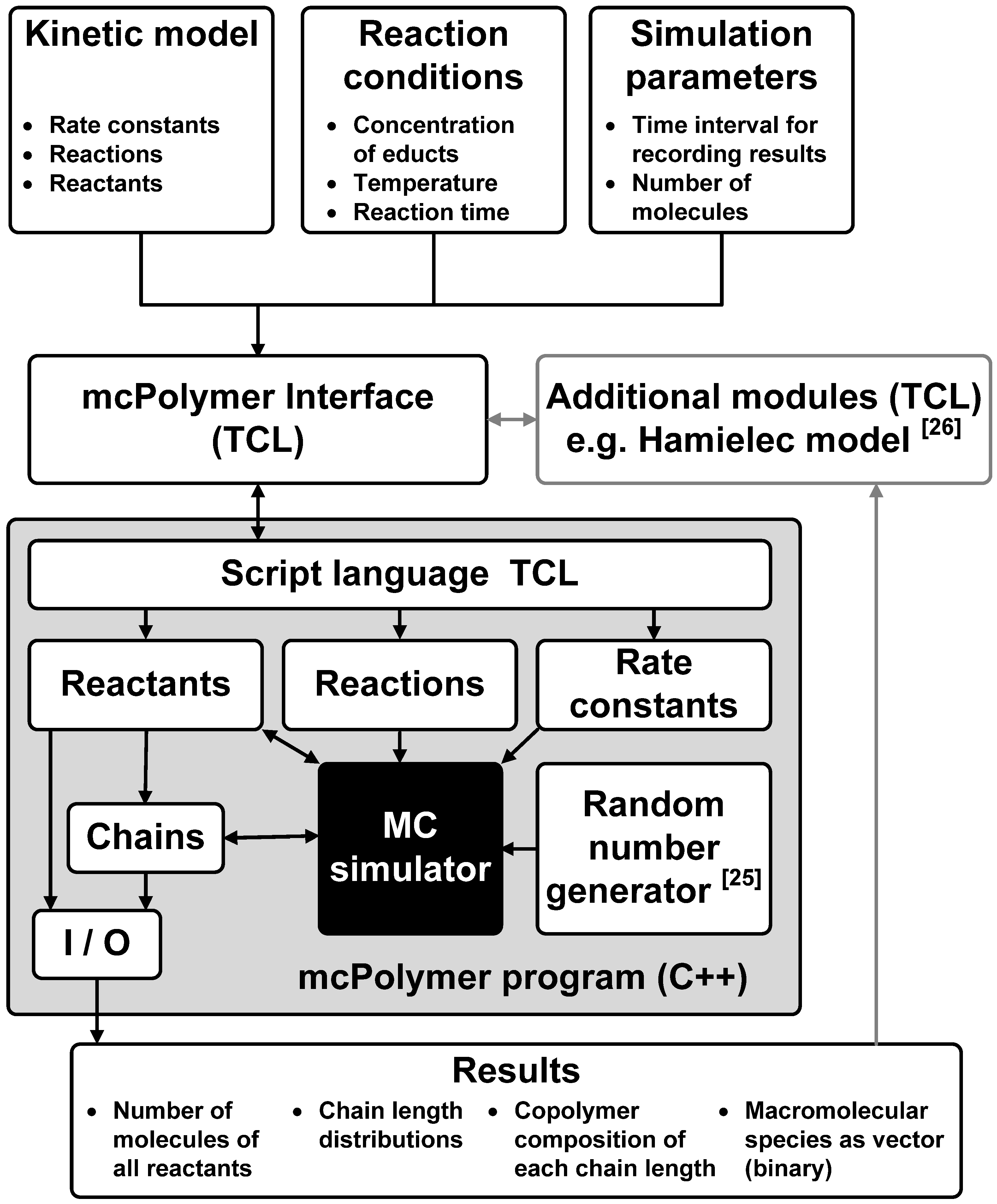
Apart from achieving a good performance of the MC simulation, another main goal of the implementation was a maximal flexibility in formulating the kinetic models and the reaction conditions. Therefore, the kinetic model was not implemented in the C++ core of the simulator, but rather as a script that is interpreted by the system. Utilizing the script language TCL, the kinetic model, the reaction conditions and the simulation parameters can be described in a flexible and readable form. The interpretation and test of plausibility is carried out by the mcPolymer Interface (TCL script). This interface initializes all objects in mcPolymer and then runs the simulation. A time interval parameter dt for writing intermediate results is set at the initialization of the simulation. Periodically completing dt, mcPolymer freezes the simulation in order to export the results as ASCII and binary files.
At this point, the interface is able to analyze the results (e.g., the conversion of educts) and modify derived reaction rate constants. An application is a periodic update of the reaction rate constant kt of the termination reaction as function of the monomer conversion for simulating the gel effect. The required calculations are not time-critical and can be provided as additional modules in the interface. For instance, it would be possible to calculate chain-length dependent rate coefficients periodically and apply them in the simulation.
Using the TCL libraries, mcPolymer itself is a TCL shell that can run TCL scripts including the mcPolymerInterface file. The interaction between the specific program modules is illustrated in
Figure 1.
Figure 1.
Software architecture of the mcPolymer simulator.
Figure 1.
Software architecture of the mcPolymer simulator.
The program mcPolymer can be initialized using intermediate results. The macromolecular species are imported from the binary files. This feature is essential in applying mcPolymer in parallel environments.
The simulation program can run on different platforms: from workstation computers with Microsoft Windows up to compute servers running UNIX (Linux). Utilizing the script language TCL for the interfaces, an integration of graphic user interfaces with data visualizing programs like gnuplot [
27] for result presentation are possible.
Along with this paper, the mcPolymer simulator is published as open source software under the GNU general public license (GPL) [
23]. The source code of mcPolymer is part of the appendix of this publication. It also contains instructions how to compile and use the software with the given example models. Anyone can modify and extend the software (e.g., adding new reaction templates). Furthermore a distribution and usage is possible observing the conditions of the GPL.
5. Simulation of Nitroxide-Controlled Homopolymerization
5.1. Kinetic Model
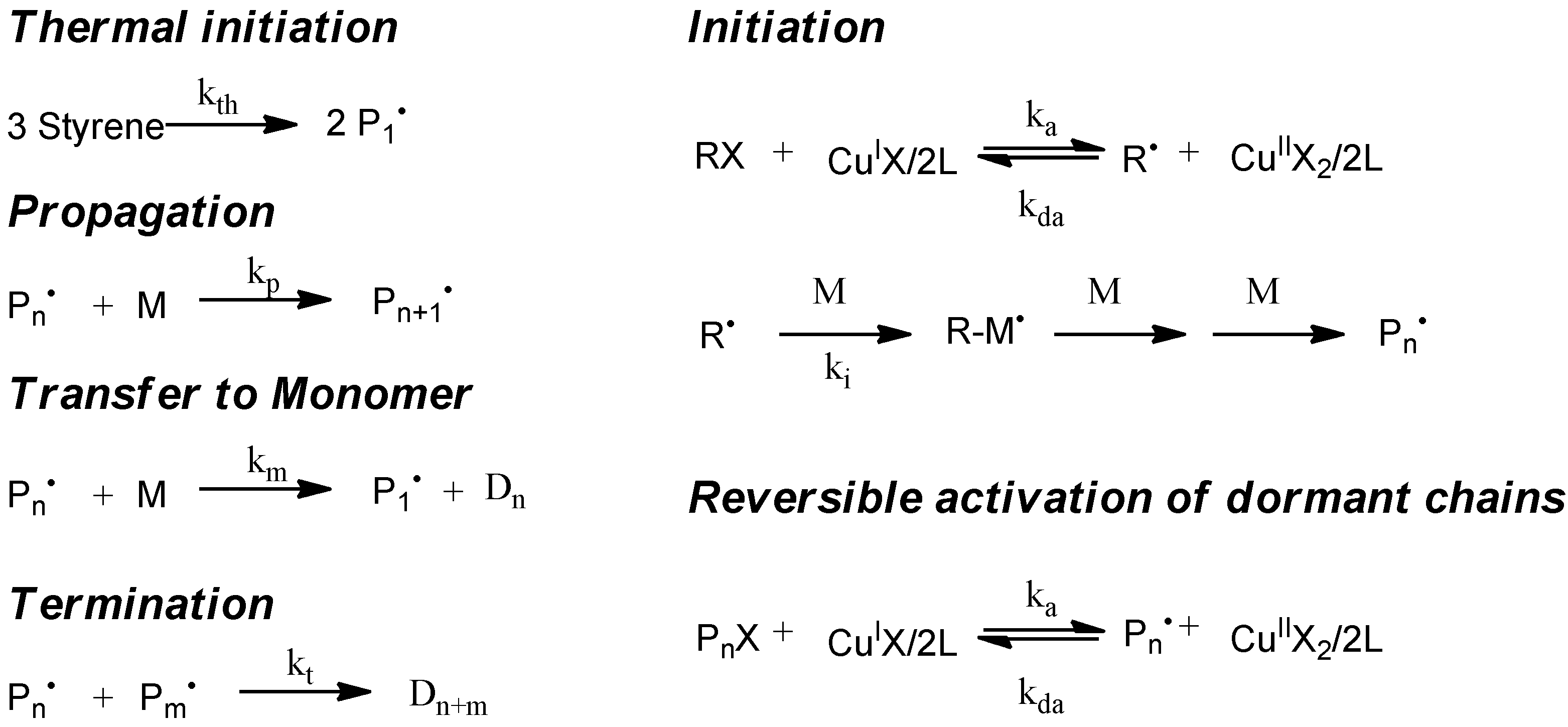
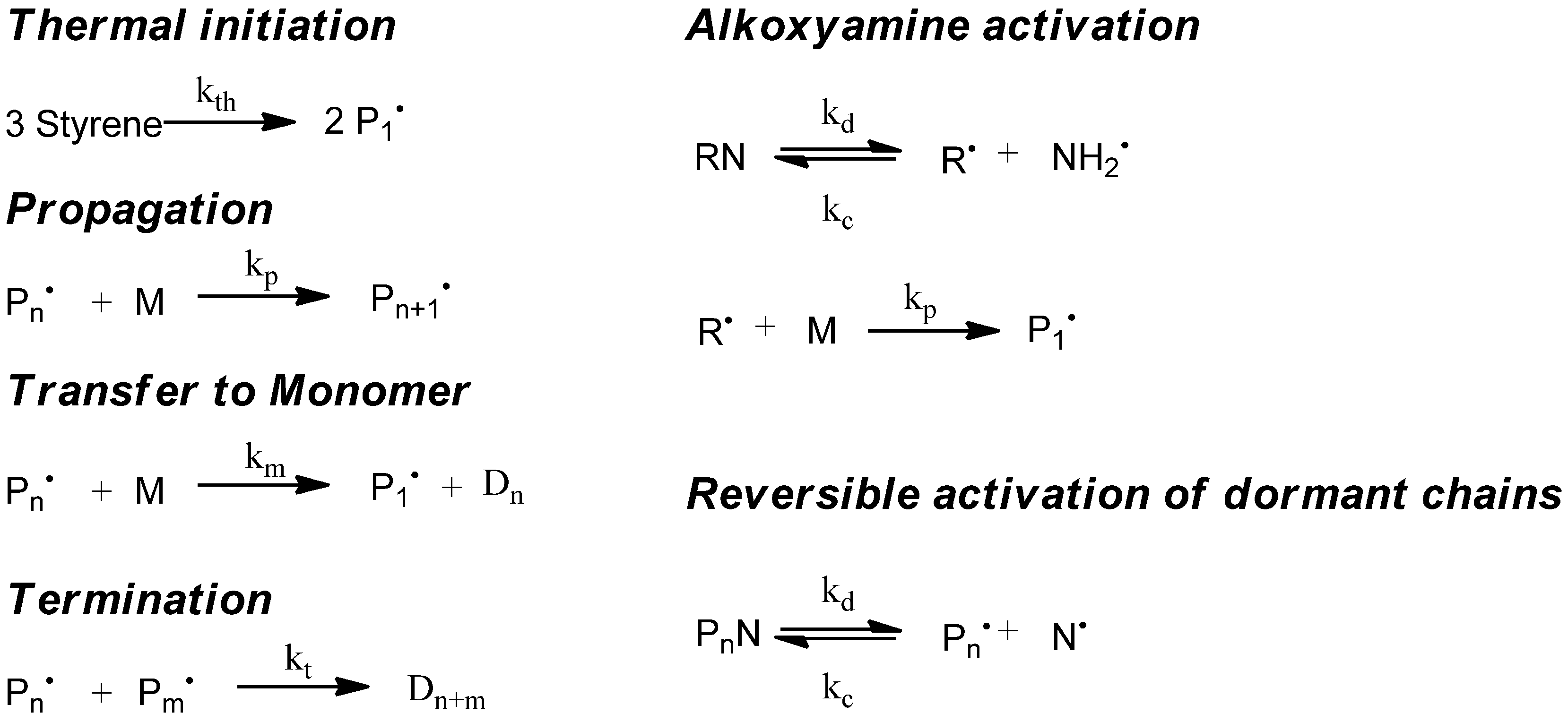
The simulation of the controlled radical polymerization with mcPolymer is exemplified first of all by a thermal-initiated nitroxide-mediated styrene homopolymerization in bulk. In addition to the reactions of the styrene homopolymerization (
Figure 2, left), the reactions of alkoxyamine activation and the equilibrium of reversible activation of dormant chains (
Figure 2, right) are required. The rate constants of styrene homopolymerization (
Table 4) are well established in the literature. For modeling the thermal initiation of styrene and the gel effect we used the empirical Hamielec model [
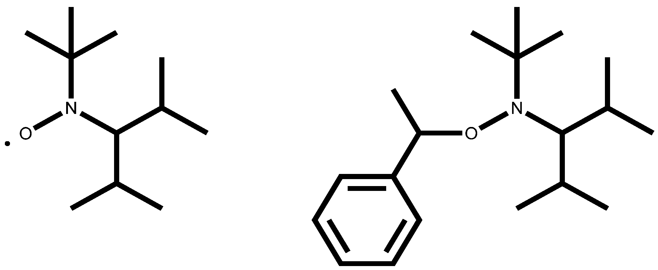
26] (Equations 13 and 14). In our simulation we applied the nitroxide 2,2,5-trimethyl-4-(isopropyl)-3-azahexane-3-oxyle (BIPNO,
Figure 3). The corresponding rate constants k
d and k
c (
Table 5) were determined using time dependent measurements of the free nitroxide and alkoxyamine concentration and applying the persistent radical effect theory [
28].
Figure 2.
Kinetic model of nitroxide mediated radical polymerization (NMP).
Figure 2.
Kinetic model of nitroxide mediated radical polymerization (NMP).
Figure 3.
Structure of nitroxide BIPNO (N) and the corresponding alkoxyamine PhEt-BIPNO (RN).
Figure 3.
Structure of nitroxide BIPNO (N) and the corresponding alkoxyamine PhEt-BIPNO (RN).
Table 4.
Rate constants of styrene homopolymerization.
Table 4.
Rate constants of styrene homopolymerization.
| Rate Constant | Value | Reference |
|---|
| kth (L2 mol−2 s−1) | 2.2 × 10⁵exp(−13810/T) | [26] |
| kp (L mol−1 s−1) | 4.2658 × 10⁷exp(−3910/T) | [29] |
| km (L mol−1 s−1) | 2.31 × 10⁶exp(−6377/T) | [26] |
| kt (L mol−1 s−1) | 2.12 × 10⁹exp(−743/T) | [30] |
Table 5.
Rate constants concerning reversible deactivation of propagating chains of styrene with nitroxide BIPNO at 123 °C.
Table 5.
Rate constants concerning reversible deactivation of propagating chains of styrene with nitroxide BIPNO at 123 °C.
| Rate Constant | Value | Reference |
|---|
| kd (s−1) | 6.8 × 10⁻³ | [28] |
| kc (L mol−1 s−1) | 6.32 × 10⁵ | [28] |
5.2. Implementation with mcPolymer
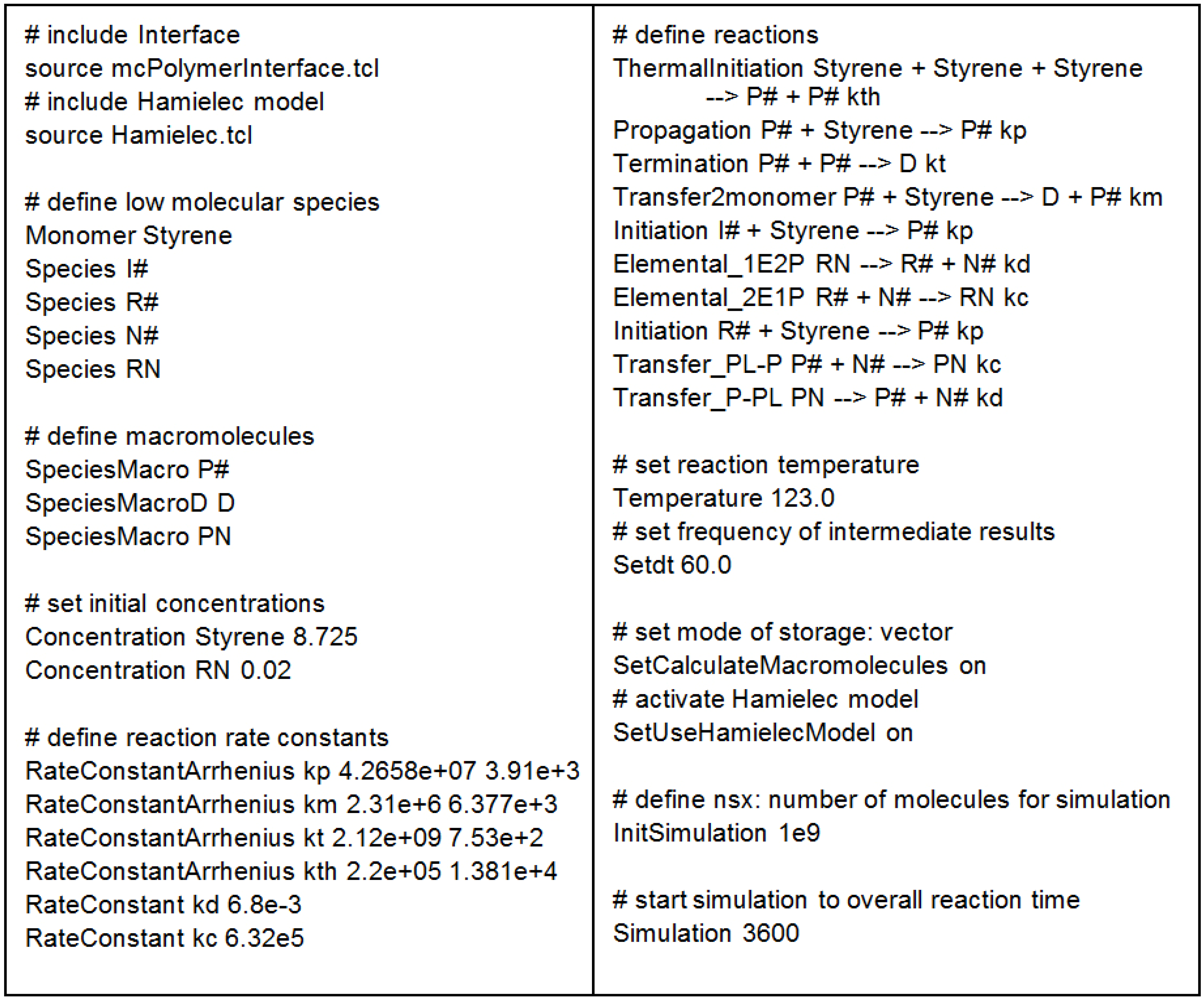
Figure 4.
TCL scheme of an exemplary mcPolymer model.
Figure 4.
TCL scheme of an exemplary mcPolymer model.
Figure 4 illustrates the simple implementation of the kinetic model as a TCL script. At first, we include the mcPolymerInferface and the Hamielec Model. Afterwards, we have to define the low molecular and macromolecular species and set their initial concentrations. The rate constants are declared as either temperature dependent or fixed. The reaction templates formulate the kinetic model using the formerly declared definitions.
InitSimulation defines the number of molecules nsx being used in the simulation. In this application, the time interval parameter dt not only defines the frequency of the output of the intermediate results, but also the time stamps for recalculating kt, applying Equations 13 and 14 as function of the monomer conversion (X).
5.3. Validation of the Monte Carlo Approach
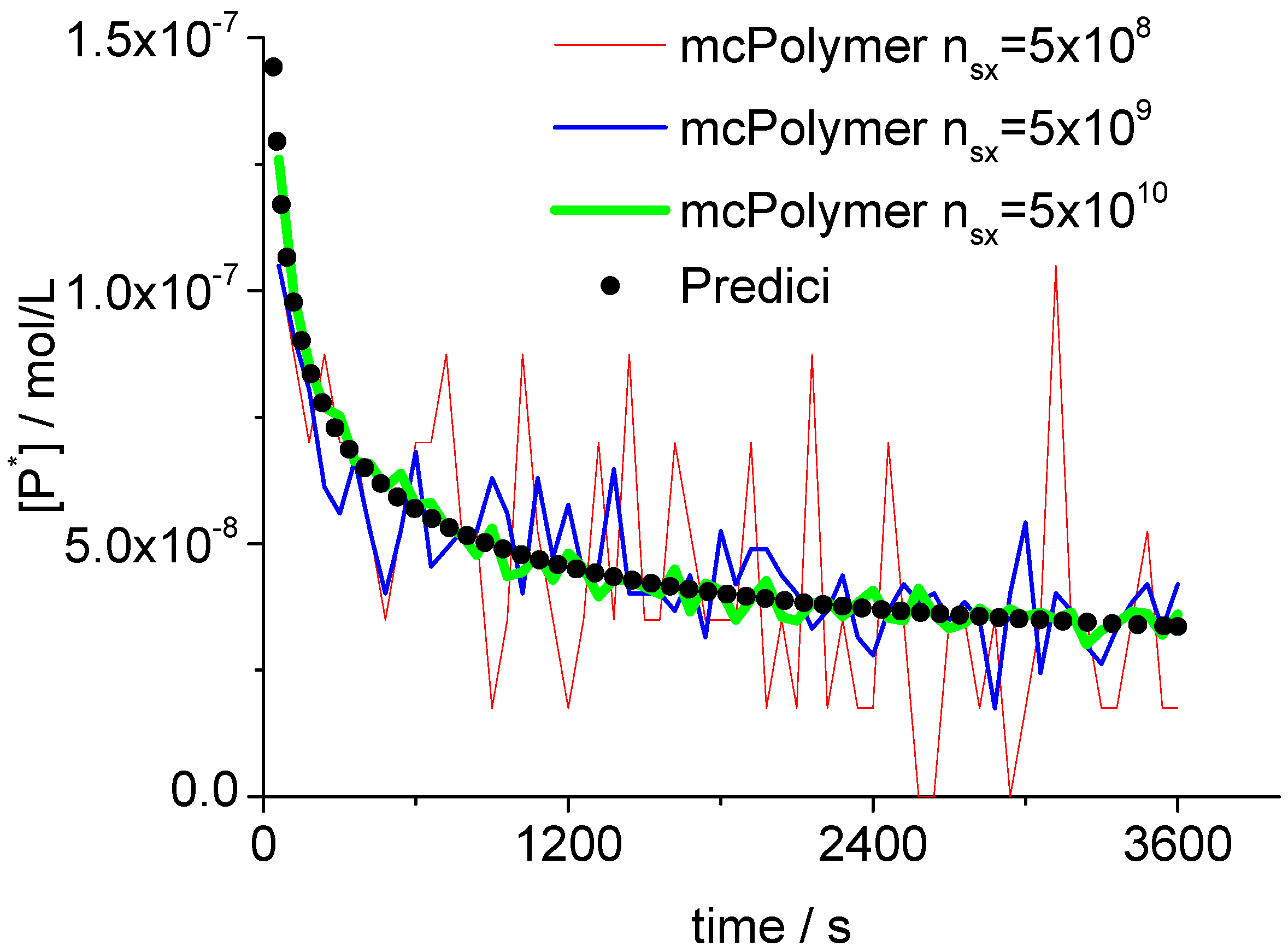
The Monte Carlo simulation only yields correct results if the concentrations of the involved species are represented by an adequate number of molecules (nsx). A general statement for the required system size cannot be made since it depends on the concrete reaction conditions. In our example, the monomer concentration scales at 101 while the radical concentration Pn· is about 10−8.
Therefore, we can derive a minimum number of 10
8 molecules for the actual simulation. Proper results considering the monomer conversion and the molar mass distribution can already be obtained with 5 × 10
8 molecules. Evoked by the persistent radical effect [
31], we are in a domain of non-stationary radical concentration. This effect does not show up until in a simulation with at least 5 × 10
9 molecules (
Figure 5). At the point of initialization (Equation 10) as well as during the simulation, the actual number of molecules is directly proportional to the total number of particles (
nsx). Here (
nsx = 5 × 10
8), the propagating polymer chains
Pn· were represented by approximately 20–70 discrete objects in the MC simulation.
Figure 5.
Concentration of propagating chains compared to PREDICI simulation results.
Figure 5.
Concentration of propagating chains compared to PREDICI simulation results.
A validation of the MC simulation can be carried out by a comparison with the simulation results of the commercial program PREDICI ([PhEt-BIPNO]0 = 0.02 mol/L; Reaction Time = 1 h). PREDICI is a deterministic differential equation solver, so the formerly discussed simulation parameter does not matter. Comparing computation performance between PREDICI and a Monte Carlo simulator are not very useful, since the computation time of the latter varies dependent on the system size, while PREDICI’s remains constant. The execution time of the model discussed here is approx. 15 seconds in PREDICI (PREDICI Version 6.20.2, Intel Core i5-650, OS: MS Windows 7).
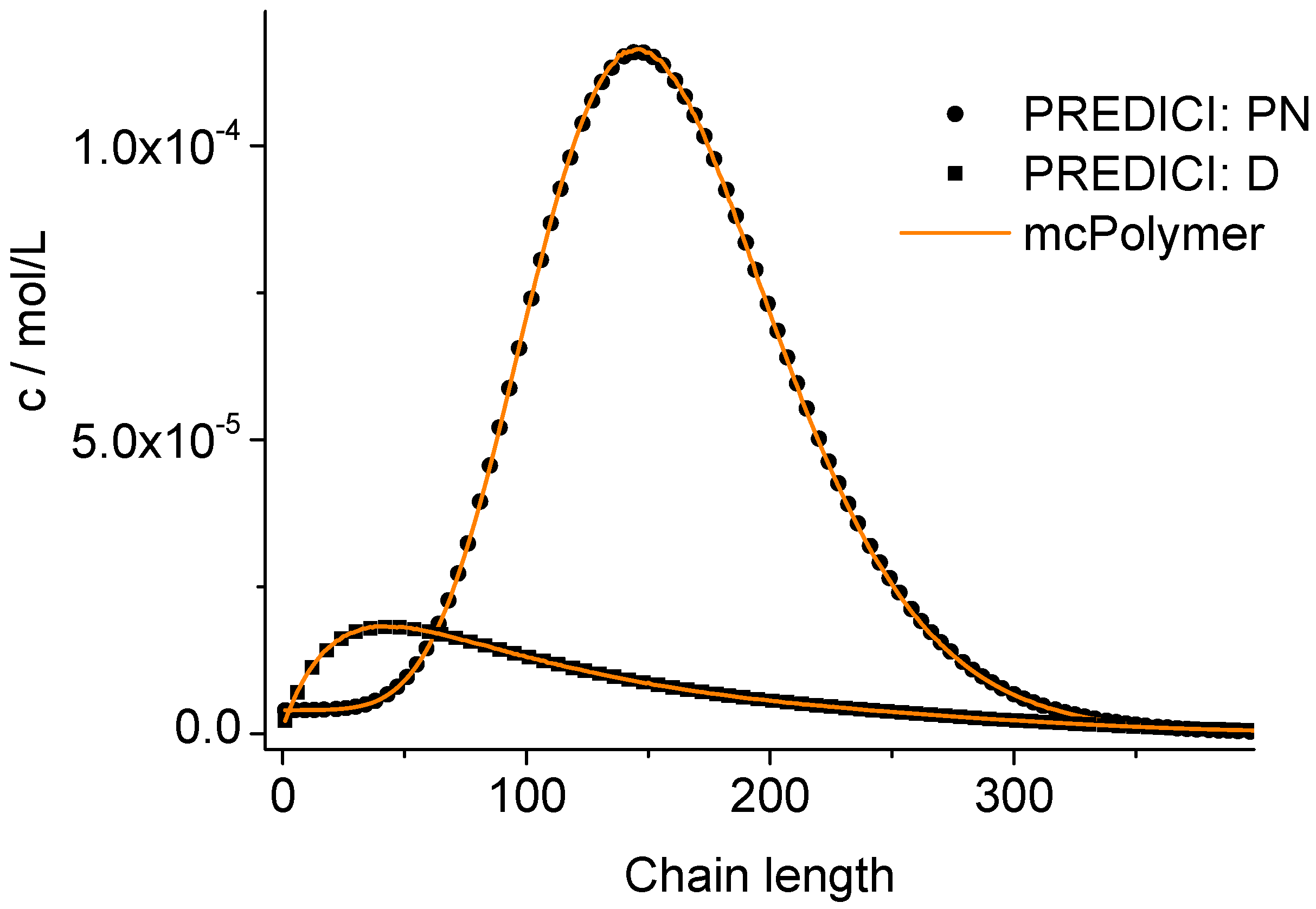
The correctness of the applied kinetic model was proven earlier on the basis of experimental data [
19]. Considering the perfect correlation between the simulation by mcPolymer and the results obtained by the PREDICI simulation (
Figure 6), we conclude a correct implementation of the kinetic model of the nitroxide-controlled polymerization with mcPolymer. Due to the comparatively high concentrations of the polymer species (PN: 1.45 × 10
−2 mol/L, D: 3.8 × 10
−3 mol/L) presented in
Figure 6, no noise appears in the chain length distribution results.
Figure 6.
Chain length distributions compared to PREDICI simulation results.
Figure 6.
Chain length distributions compared to PREDICI simulation results.
5.4. Performance Analysis
The computation time depends on the number of molecules (
nsx), the mode of storage of the macromolecular species (histogram/vector), and the concentration of the reactants. In addition to the mere computation time, the speed performance of the simulation can be rated by the number of Monte Carlo steps executed per second. We introduced this performance parameter with the first application of mcPolymer [
17]. Later on, it was used by Barmer Kowollik
et al. [
18] for benchmarking parallelized Monte Carlo simulations and by Broadbelt
et al. [
32] for performance analysis of nitroxide-controlled copolymerization.
The performance analysis has been processed on the following two systems:
2 AMD Opteron 6134 Magny Cours CPU (16 cores, 2.2 GHz), 128 GB RAM, OS: Open SuSE Linux 11.4, compiler: GNU Compiler Collection (gcc) 4.5.1→Linux-Opteron;
1 Intel Core i5-650 Clarkdale (2 Cores, 3.2–3.46 GHz), 16 GB RAM, OS: MS Windows 7 Enterprise 64 bit, compiler: Visual Studio 2010 Ultimate 64 bit →Windows-Core i5.
The results of the test runs are summarized in
Table 6 and
Table 7. As one can see, the number of MC steps is directly proportional to the system size
nsx. Due to persistent radical effect, the radical concentration is not constant and depends on the initial concentration of the alkoxyamine. Therefore, at the same reaction time and higher alkoxyamine concentration, a higher monomer conversation is achieved and thus more Monte Carlo steps are required.
Table 6.
Performance analysis on the Linux-Opteron system, reaction time = 1 h.
Table 6.
Performance analysis on the Linux-Opteron system, reaction time = 1 h.
| nsx | [PhEt-BIPNO]0 = 0.02 mol/L | [PhEt-BIPNO]0 = 0.01 mol/L |
|---|
| MC steps | Time/s | MCpsec/s−1 | MC steps | Time/s | MCpsec/s−1 |
|---|
| 1 × 10⁹ | 3.85 × 10⁸ | 108 | 3.53 × 10⁶ | 2.85 ×10⁸ | 24 | 3.91 × 10⁶ |
| 5 × 10⁹ | 1.92 × 10⁹ | 559 | 3.43 × 10⁶ | 1.42 × 10⁹ | 122 | 3.88 × 10⁶ |
| 1 × 10¹⁰ | 3.85 × 10⁹ | 1174 | 3.28 × 10⁶ | 2.85 × 10⁹ | 250 | 3.79 × 10⁶ |
| 5 × 10¹⁰ | 1.92 × 10¹⁰ | 6156 | 3.12 × 10⁶ | 1.42 × 10¹⁰ | 1273 | 3.73 × 10⁶ |
| 1 × 10¹¹ | 3.85 × 10¹⁰ | 13239 | 2.91 × 10⁶ | 2.85 × 10¹⁰ | 2621 | 3.62 × 10⁶ |
Table 7.
Performance analysis on the Windows-Core i5 system; [PhEt-BIPNO]0 = 0.02 mol/L, reaction time = 1 h.
Table 7.
Performance analysis on the Windows-Core i5 system; [PhEt-BIPNO]0 = 0.02 mol/L, reaction time = 1 h.
| nsx | MC steps | Vector storage mode | Histogram mode |
|---|
| Time/s | MCpsec/s−1 | Time/s | MCpsec/s−1 |
|---|
| 1 × 10⁹ | 3.85 × 10⁸ | 61 | 6.31 × 10⁶ | 73 | 5.27 × 10⁶ |
| 5 × 10⁹ | 1.92 × 10⁹ | 319 | 6.03 × 10⁶ | 357 | 5.39 × 10⁶ |
| 1 × 10¹⁰ | 3.85 × 10⁹ | 685 | 5.61 × 10⁶ | 711 | 5.41 × 10⁶ |
| 5 × 10¹⁰ | 1.92 × 10¹⁰ | 3689 | 5.21 × 10⁶ | 3568 | 5.39 × 10⁶ |
| 1 × 10¹¹ | 3.85 × 10¹⁰ | – | – | 7140 | 5.39 × 10⁶ |
Since the simulation program is executed on one CPU core only, it is not surprising that the Windows system runs faster due to the higher CPU clocking. Using the vector storage mode for the macromolecular species, the program performance increases due to the simpler selection of the macromolecules, but leads to a massive increase of the memory requirements (each polymer object has to be stored individually in the RAM). The latter depend on the initial concentration of the alkoxyamine and the simulation parameter nsx. Taking the example of [BIPNO]0 = 0.02 mol/L and nsx = 1010, the memory requirements are up to 2.1 GB RAM in vector storage mode compared to 0.014 GB RAM in histogram mode.
The number of Monte Carlo steps executed per seconds (MCpsec) remains constant during the simulation in histogram mode, while it decreases in vector mode. We assume the reason might lie in the increasing number of cache misses. An indication is the stronger correlation between MCpsec und nsx on the Windows system.
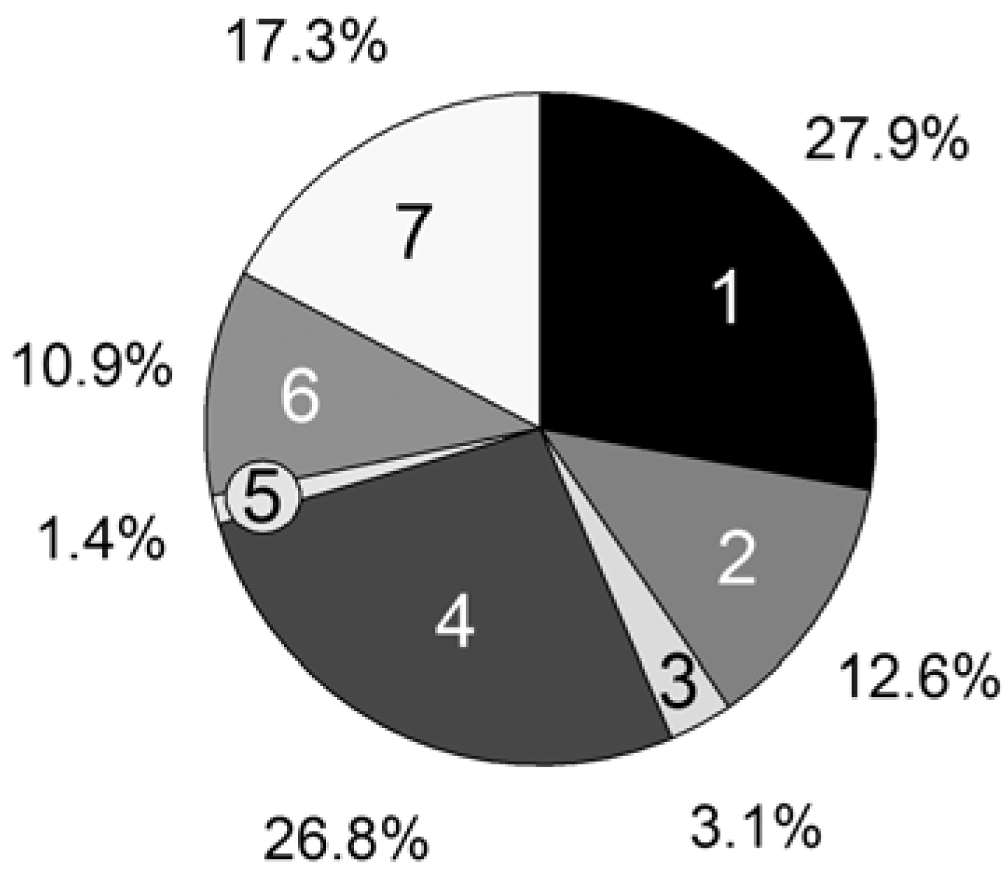
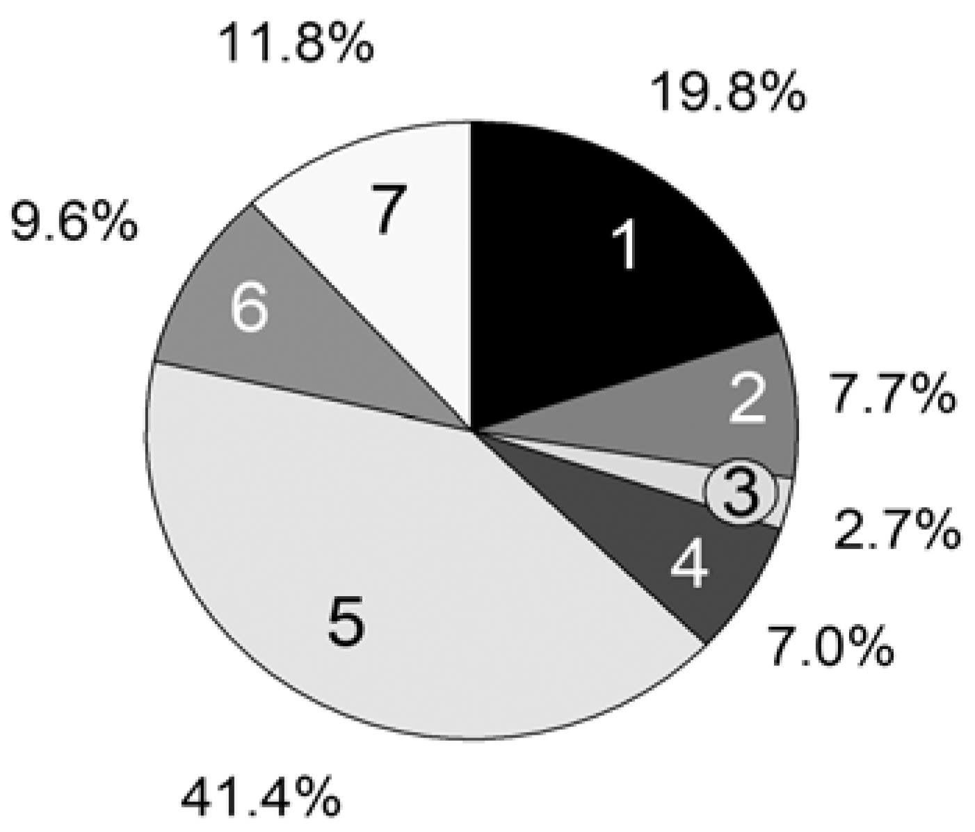
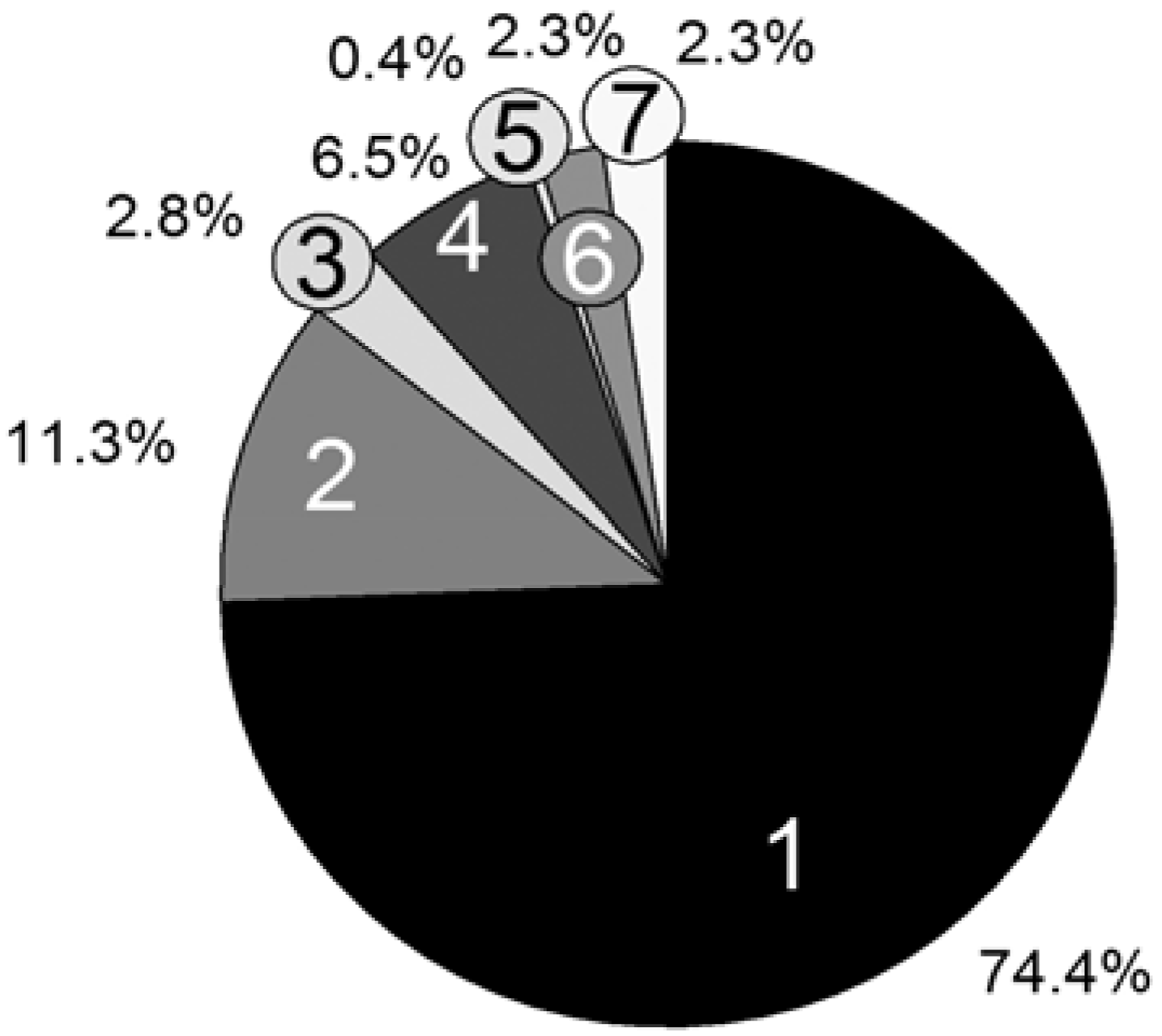
For further improvements of our program, we analyzed the statistical time consumption of the particular parts of a MC simulation step. Using the CPU profiler of the Google Performance Tools [
33], we could measure the computation time of every single line of code. The following relevant parts are summarized in
Figure 7:
1. Update of the reaction rates Rvand probabilities pv (Equations 2, 6–8);
2. Choice of a reaction (Equation 1);
3. Particle numbers of the reactants Xi are changed by consuming the educts and creating the products;
4. Execution of the propagation reaction;
5. Execution of the Transfer_PL-P reaction;
6. Execution of the Transfer_P-PL reaction;
7. Calculation of the time interval (Equation 9).
For the computation time only, the propagation reaction and the reversible deactivation of the propagating chain by the nitroxide are important, while all other reactions are negligible. Remarkable is the large difference between the reactions Transfer_PL-P (5) and Transfer_P-PL (6), which are performed almost equally as often. The reason is the vast concentration difference between the propagating chain (macromolecular educt in Transfer_PL-P) and the dormant chains (macromolecular educt in Transfer_P-PL). The number of propagating chains is comparatively small and can be kept in cache, causing a very fast individual educt molecule selection.
Figure 7.
Persistence simulation time; [PhEt-BIPNO]0 = 0.02 mol/L, Reaction Time = 1 h; Vector storage mode; 1: Update Rv and pv; 2: Reaction choice; 3: Execute reaction (Xi); 4: Propagation; 5: Transfer_PL-P; 6: Transfer_P-PL; 7: Calculate τ.
Figure 7.
Persistence simulation time; [PhEt-BIPNO]0 = 0.02 mol/L, Reaction Time = 1 h; Vector storage mode; 1: Update Rv and pv; 2: Reaction choice; 3: Execute reaction (Xi); 4: Propagation; 5: Transfer_PL-P; 6: Transfer_P-PL; 7: Calculate τ.
6. Simulation of ATRP Homopolymerization
6.1. Kinetic Model and Implementation with mcPolymer
The presented kinetic model of the ATRP polymerization is well-known in the literature. Matyjaszewski
et al. published a modeling approach of chain-end functionality in atom transfer radical polymerization using PREDICI [
34,
35]. Based on these models, Soares
et al. introduced a Monte Carlo simulation of ATRP [
14]. It was validated with experimental data and by the simulation method of moments. Its implementation with MATLAB only allowed comparatively small molecule numbers (
nsx up to 2.7 × 10
7). This model was extended to the simulation of ATRP with bifunctional initiators [
15] and to the modeling of the semibatch copolymerization [
36]. Najafi
et al. utilized the ATRP model for simulating the chain-length dependent termination [
37].
Figure 8 illustrates the applied model of ATRP polymerization. The styrene homopolymerization and the corresponding reaction rates (
Table 4) were used identically as in the NMP model presented earlier.
The specific reactions of ATRP on the right side of the scheme were implemented by two elemental reactions using template ‘Elemental_2E2P’; One reaction applying template ‘Initiation’ and two transfer reactions of the macromolecular species using the template ‘Transfer_PL-PL’. All templates were introduced in
Table 2. The required reaction rate constants (
Table 8) were experimentally determined by Fukuda
et al. [
38] (k
a) and Matyjaszewski
et al. [
39] (K = k
a/k
d) for the catalyst Cu
IX/2L (X: Br, L: 4,4'-di-
n-heptyl-2,2'-bipyridine).
Figure 8.
Kinetic model of atom transfer radical polymerization (ATRP).
Figure 8.
Kinetic model of atom transfer radical polymerization (ATRP).
Table 8.
Rate constants concerning reversible activation of dormant chains at 110 °C.
Table 8.
Rate constants concerning reversible activation of dormant chains at 110 °C.
| Rate Constant | Value | Reference |
|---|
| ka (L mol−1 s−1) | 4.5 × 10⁻¹ | [38] |
| kda (L mol−1 s−1) | 1.1 × 10⁷ | [39] |
7. Simulation of RAFT Polymerization
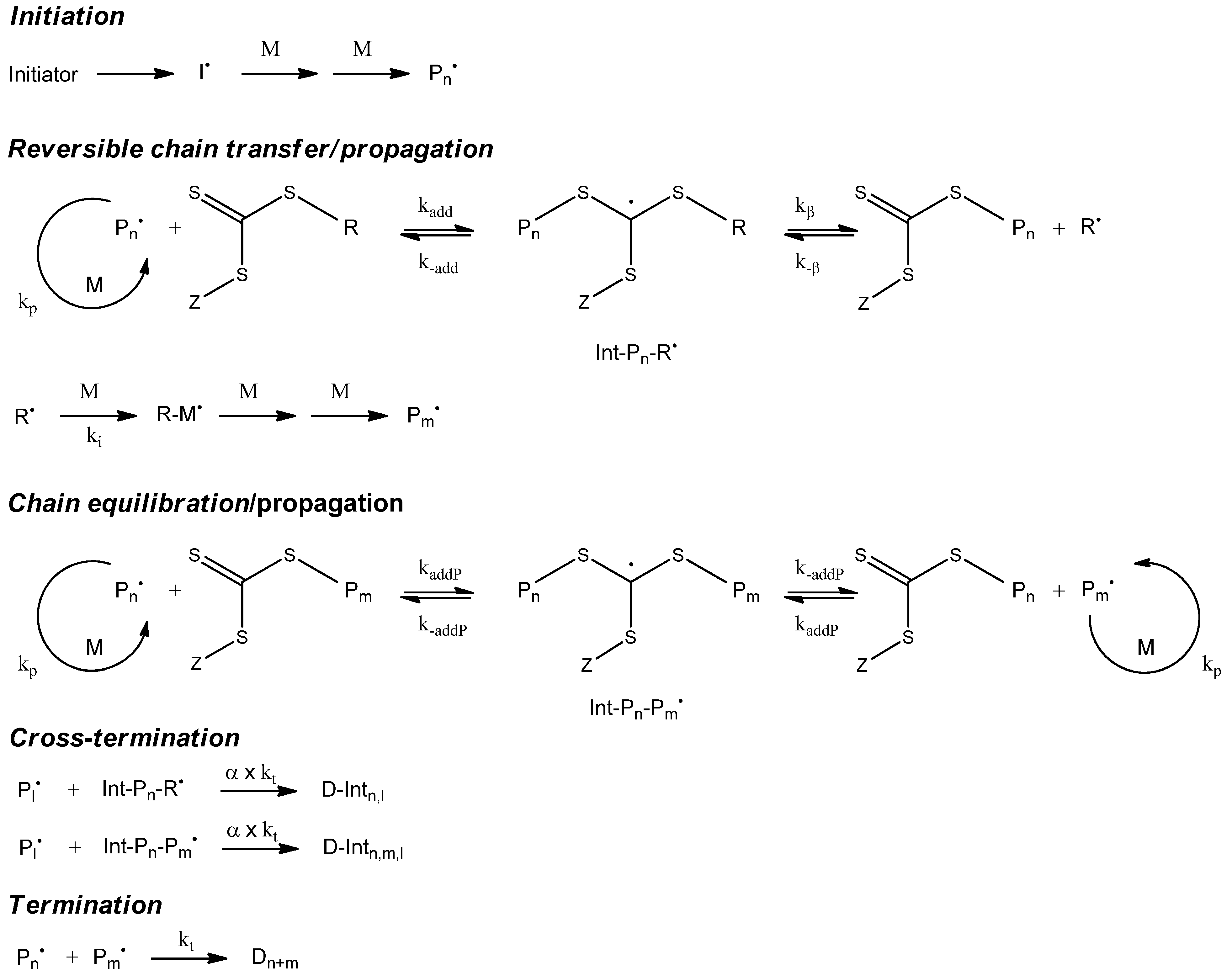
7.1. Kinetic Model
The kinetic model of the Cumyl dithiobenzoate (CDB) mediated methyl acrylate (MA) RAFT polymerization that we applied is illustrated in
Figure 10. We determined the corresponding reaction rates (
Table 10) by fitting the model to the experimental data [
17]. As a side reaction, the model contains a cross termination between the propagating chain and the intermediate radical of the RAFT equilibrium. The ongoing discussion “cross termination
vs. stable intermediate model” [
40,
41,
42,
43,
44] is not the subject of this paper. Perrier
et al. demonstrated that both approaches were able to describe the experimental data of the RAFT polymerization adequately [
41].
Table 10.
Rate constants cumyl dithiobenzoate mediated methyl acrylate homopolymerization.
Table 10.
Rate constants cumyl dithiobenzoate mediated methyl acrylate homopolymerization.
| Rate constant | Value | Reference |
|---|
| ki (s−1) | 2.89 × 10¹⁵exp(−15663/T) | [45] |
| f | 0.64 | [46] |
| kp (L mol−1 s−1) | 3.61 × 10⁶exp(−1671/T) | [47] |
| kt (L mol−1 s−1) | 1.59 × 10¹⁰exp(−1082/T) | [48] |
| kadd (L mol−1 s−1) | 3.06 × 10⁸ | [17] |
| k-add (s−1) | 20 × 9 | [17] |
| kaddP (L mol−1 s−1) | 9.36 × 10⁶ | [17] |
| k-addP (s−1) | 784 | [17] |
| α | 0.15 | [17] |
Figure 10.
Kinetic model of reversible addition fragmentation chain transfer polymerization (RAFT)polymerization.
Figure 10.
Kinetic model of reversible addition fragmentation chain transfer polymerization (RAFT)polymerization.
The validation of the kinetic model was performed [
17] using experimental data measuring the monomer conversion as function of time, the full molecular weight distributions, and the concentrations of the intermediate RAFT radical with experimental electron spin resonance spectroscopic data.
7.2. Implementation with mcPolymer
The RAFT polymerization is an example for the advantages of Monte Carlo methods when simulating polymerization models containing complex macromolecular species. In the main equilibrium of the RAFT polymerization, a species with two polymer chains appears as an intermediate radical. During a MC simulation, we can conserve both polymer chains in a molecular object and, therefore, are able to model a fragmentation of this molecule quite simply.
The mcPolymer interface offers the macromolecular species “SpeciesMacro_P-O-P” (
Table 1) for modeling the intermediate radical in the main equilibrium. During the cross termination reaction, a three-arm star polymer is created, which is represented by a macromolecular object of type “SpeciesMacro_P-O<PP” (
Table 1).
For modeling the pre-equilibrium, we can use the reaction templates “Transfer_PL-P” and “Transfer_P-PL” as we have already used them for the NMP, while the main equilibrium of the RAFT polymerization can be implemented utilizing the templates “ChainAddition” and “ChainFragmentation” (
Table 1).
In contrast to mcPolymer, RAFT polymerization simulations with PREDICI have to simulate every polymer chain separately as a unique pseudo species [
9]. This approach also leads to correct results [
10], but the analyses are more complex.
As a conclusion, simulating RAFT polymerizations with mcPolymer offers a deep view inside the complex macromolecular structures using a straight model representation, while the produced results are simple for handling and analyses.
7.3. mcPolymer in Parallel Environments
Barner-Kowollik
et al. presented a parallel high performance Monte Carlo simulation approach for complex polymerization using the example of RAFT polymerization [
18]. In this paper, the simulation was compared to PREDICI regarding the influence of the following simulation parameters: the system size (
nsx range between 1 × 10
9 and 1 × 10
10 particles), the number of parallel processes (4 to 16), and the reaction time between synchronization (2 to 500 s). It was not surprising that the only important factor was the number of particles available for each process. As long the number is large enough to remain in the continuum, the simulation provides correct results independent of the synchronization time.
We implemented a parallel simulation of the formerly discussed RAFT polymerization model with mcPolymer. The system size was set up in the range of 1 × 10
9–2.5 × 10
10 for each process (10 processes total). After a fixed synchronization time, all molecules, including the complex macromolecular objects are collected, mixed up, and statistically redistributed over the processes. Each process requires approx. 2.5 GB of RAM in vector storage mode (
nsx = 1 × 10
10, 10 processes). Therefore, 25 GB have to be shifted at every single synchronization step. The results in
Table 11 make obvious that synchronizations after every 5 min of reaction time (12 cycles) determine the speed of the whole simulation. The simulation was executed with overall 10
11 molecules in 11723 s. The results agree with those obtained in a single process set up with 10
11 particles, but the latter required 86897 s. In our test runs we could not detect an influence of the synchronization time on the simulation results, which leads to the conclusion that we can generally omit the synchronization steps and merge the individual results (chain length distribution) at the end. The results are qualitatively the same as in the single process—as long as the precondition of every simulation process remaining in the continuum is fulfilled. The speed-up factor reaches 14.3 with 10 processes (
Table 11).
Using parallelization, a large number of molecules can be obtained, which can be used to smooth all concentration-time curves. Additionally, the number of polymer species used for statistical analysis is increased. Unfortunately, the underlying single MC simulation is not accelerated, since it still needs a certain system size.
An effective acceleration could be achieved, if we were able to parallelize each Monte Carlo step. As an example, the calculation of the reaction probabilities could be processed in parallel. Since the sequential part of a Monte Carlo step is over 50 percent of the time consumption and the mean execution time of a MC step (e.g., 5.5 × 10⁻⁷ s from 1.81 × 10⁶ MC steps/s; nsx = 5 × 10⁹) is in dimension of the memory synchronization between the processes, the attempt of parallelization at the level of a single MC step and the common x86 CPU architecture is futile.
Table 11.
Performance analysis in parallel environments (10 processes); Reaction time = 1 h; Linux-Opteron; [CDB]0 = 0.025 mol/L; [MA]0, = 11.04 mol/L.
Table 11.
Performance analysis in parallel environments (10 processes); Reaction time = 1 h; Linux-Opteron; [CDB]0 = 0.025 mol/L; [MA]0, = 11.04 mol/L.
| System size
nsx of one process | Overall system size | Synchronization cycles | Parallel simulation time/s | Sequential synchronization time/s | Overall simulation time/s |
|---|
| 1 × 10⁹ | 1 × 10¹⁰ | 12 | 817 | 317 | 1134 |
| 1 × 10⁹ | 1 × 10¹⁰ | 24 | 1059 | 669 | 1728 |
| 1 × 10⁹ | 1 × 10¹⁰ | 60 | 1826 | 1692 | 3518 |
| 1 × 10¹⁰ | 1 × 10¹¹ | 12 | 8453 | 3270 | 11723 |
| 1 × 10¹⁰ | 1 × 10¹¹ | 24 | 8974 | 6741 | 15715 |
| 2.5 × 10¹⁰ | 2.5 × 10¹¹ | 12 | 23022 | 9423 | 32445 |
8. Simulation of Nitroxide-Controlled Copolymerization
8.1. Kinetic Model
A nitroxide-controlled homopolymerization of methyl methacryclate (MMA) is not possible due to the degradation of nitroxide by H-abstraction [
49]. The SG1-controlled radical copolymerization of MMA and styrene (S) is therefore of particular interest, since Charleux
et al. [
50] demonstrated the possibility of performing a nitroxide-controlled polymerization of methyl methacrylate with a small amount of styrene. Besides experimental work, the influence of the copolymer styrene was analyzed by model calculations [
51]. Charleux
et al. implemented the copolymerization model in PREDICI considering the penultimate effect [
51]. Furthermore, Broadbelt
et al. created Monte Carlo models of SG1-controlled MMA/S copolymerization, examining the copolymer composition and sequence effects [
20,
21,
22].
We implemented the model of SG1 controlled MMA/S copolymerization published by Charleux
et al. [
51]. It contains the following reactions:
Dissociation equilibrium of the SG1-alcoxyamine;
Initiation of new polymer chains in consideration of the first two monomer units for modeling the penultimate effect;
Combination reactions of low molecular radicals;
Propagation reactions;
Reversible deactivation of propagating chains by the nitroxide SG1;
Termination of macromolecules by combination and disproportionation;
β-hydrogen transfer from propagating macroradicals with chain end MMA to nitroxide SG1.
Formulating the entire 52 reactions and 37 reaction rate constants along with their references would go beyond the scope of this paper and can be found in the appendix of the publication by Charleux
et al. [
51] and in our appendix material as mcPolymer model (Appendix-5-Example-SG1-MMA-S-copolymerization.tcl). The initial concentrations of the reactants are: [MMA]
0 = 8.48 mol/L, [Styrene]
0 = 0.82 mol/L, [SG1-alcoxyamine]
0 = 0.0273 mol/L and [SG1]
0 = 0.00274 mol/L.
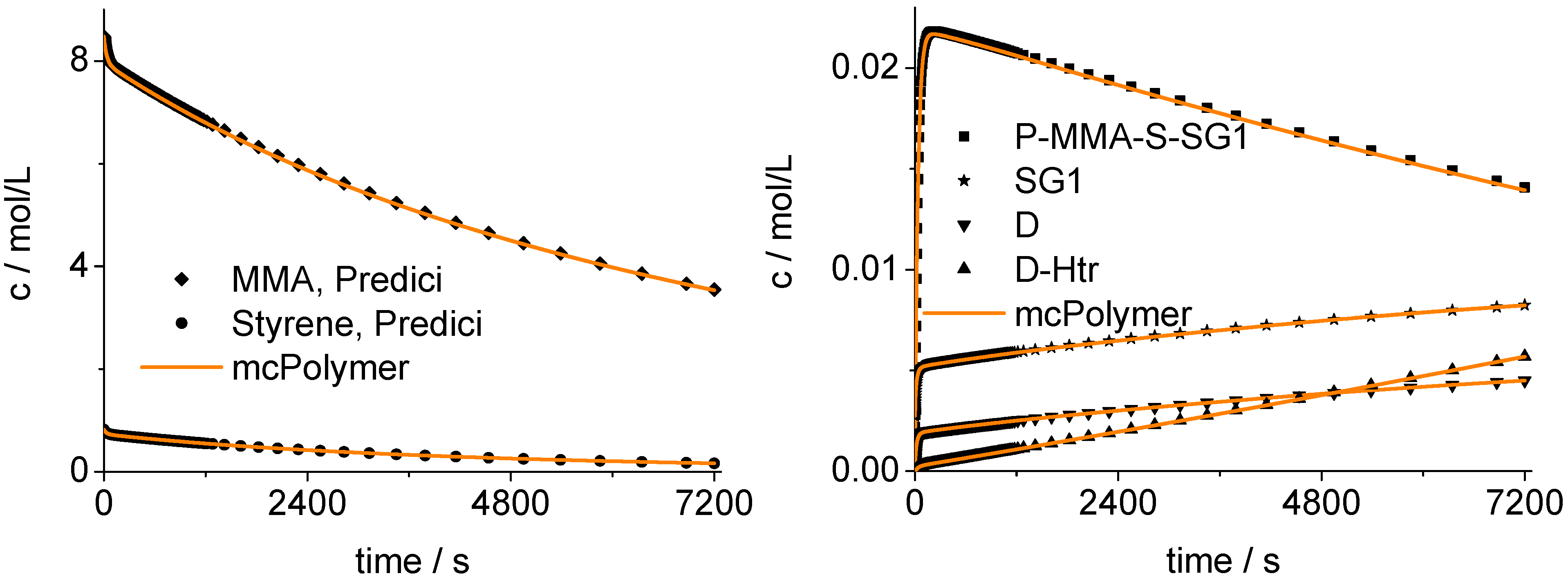
8.2. Validation of the Monte Carlo Approach
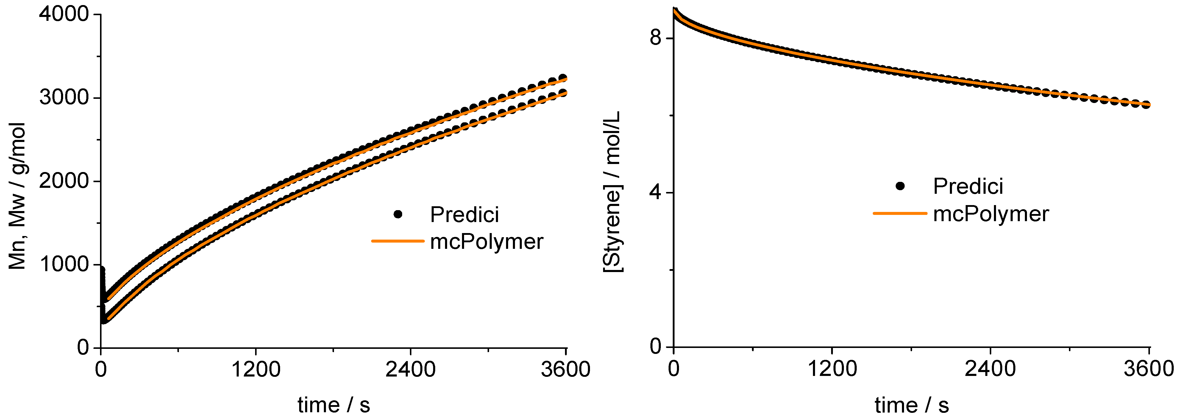
The mcPolymer simulation was validated using a PREDICI model. We examined the time-dependent concentrations of the MMA and S comonomers (
Figure 12) and, therefore, the copolymer composition.
Figure 12 shows the agreement of our implementation (mcPolymer) with the PREDICI model considering the concentration-time profile of the essential reactants of the polymerization:
The nitroxide: SG1;
The SG1 terminated polymer chains with a chain end sequence MMA-S: P-MMA-S-SG1;
The dead polymers resulting from termination reactions: D;
The dead polymers formed by ß-hydrogen transfer from propagating macroradicals withchain end MMA to nitroxide SG1: D-Htr.
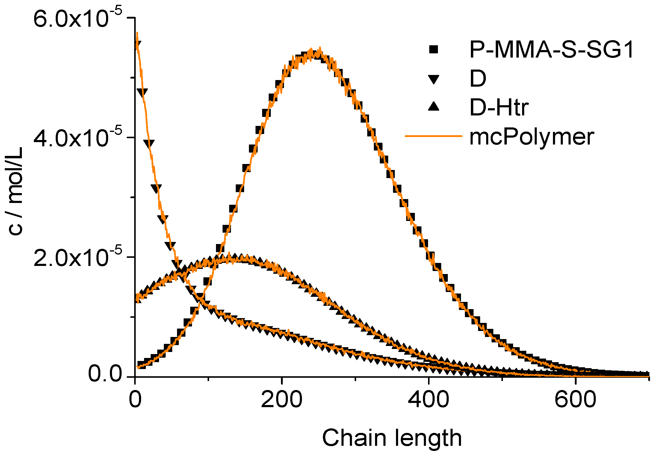
The chain length distributions of the products P-MMA-S-SG1, D and D-Htr determined after two hour reaction time also results in a perfect correlation between our simulator and the PREDICI model (
Figure 13).
Figure 12.
Validation of mcPolymer with PREDICI: Concentration-time-profiles.
Figure 12.
Validation of mcPolymer with PREDICI: Concentration-time-profiles.
Figure 13.
Validation of mcPolymer with PREDICI: Chain length distributions.
Figure 13.
Validation of mcPolymer with PREDICI: Chain length distributions.
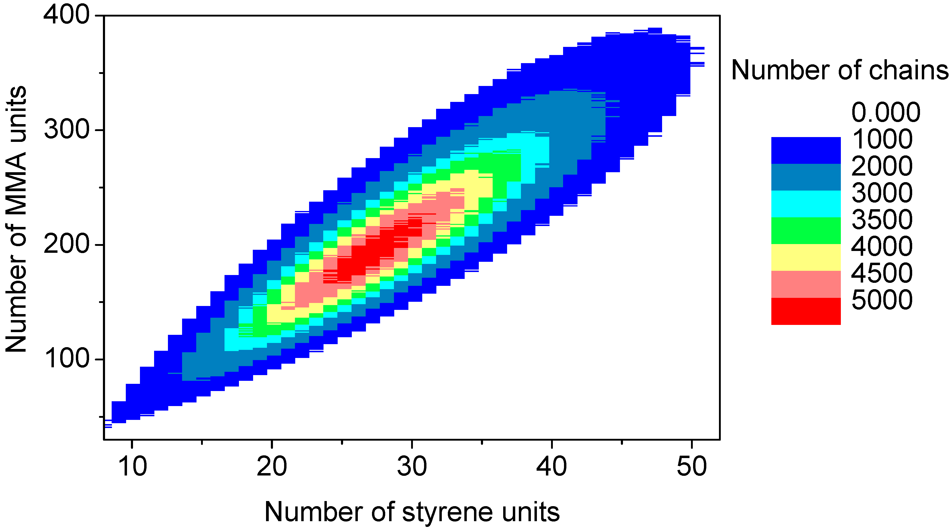
8.4. Analysis of Simulation Results
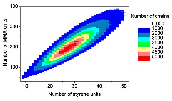
The discrete recording of the composition of each polymer chain offers a thorough analysis of the molecular and chemical structure of the polymers formed by the copolymerization. Contour plots (
Figure 15) are an example of coupled breakdown of chain length and copolymer composition of polymers, known from the MALDI-TOF analytic of copolymers [
52,
53]. The addition of the number of styrene units (
x-axis) with the number of MMA units (
y-axis) results in the chain length of the corresponding data point. Due to the concentration relation in the reaction solution and the reactivity ratios ([MMA]
0 = 8.48 mol/L, [styrene]
0 = 0.82 mol/L, r
MMA/S = 0.420 [
52], r
S/MMA = 0.517 [
52]), MMA is predominantly built in in the polymer chain. Since the simulation was performed with a large number of molecules (
nsx = 5 × 10
10), the frequency distributions are well separated. The chain length and composition distribution of a total number of 1.5 × 10
7 polymer chains is presented in this plot.
Figure 15.
Contour plot: Coupling copolymer composition with chain length distribution.
Figure 15.
Contour plot: Coupling copolymer composition with chain length distribution.
9. Conclusions
In this paper, a Monte Carlo simulation program named mcPolymer for simulating radical polymerizations was presented. It was provided as an open source project under the GPL license. Our mcPolymer simulator runs on MS Windows and Linux platforms. Regarding the intensive memory consumption, it is recommended to use 64 bit systems.
The software architecture of mcPolymer was introduced focusing on the data management of polymer chains. Due to the flexible interface, the formulation of complex polymerization models and the setup of its reaction conditions are quite simple.
The application was demonstrated on examples of controlled radical polymerizations (nitroxide-controlled, ATRP, RAFT, nitroxide-controlled copolymerization). We relied on formerly published models validated by experimental data. Using the example of RAFT polymerization, we discussed applying mcPolymer in parallel environments. The example of nitroxide-controlled copolymerization demonstrated how to also obtain the copolymer composition of each polymer chain along with molar mass distribution as a simulation result.
PREDICI models were used for validating the MC program. A crucial point of Monte Carlo simulations for modeling radical polymerization, is the system size. Different possibilities were exemplarily illustrated for finding an adequate balance between precision and computation time of the simulation.
For all examples of controlled radical polymerization, we presented detailed performance analyses demonstrating the influence of the system size, concentrations of reactants and, therefore, of the dormant chains, as well as the peculiarities of data management, and the CPU architecture.
mcPolymer is a powerful tool for simulating controlled radical polymerizations. Due to its flexible software architecture and interface, new reaction templates can easily be implemented and, thus, be adjusted to further polymerization models.


