Article

PRINCEPS: A Computer-Based Approach to the Structural Description and Recognition of Trends within Structural Databases, and Its Application to the Ce-Ni-Si System

Department of Chemistry, University of Wisconsin—Madison, 1101 University Avenue, Madison, WI 53706, USA
*
Author to whom correspondence should be addressed.
Crystals 2016, 6(4), 35; https://doi.org/10.3390/cryst6040035
Submission received: 6 December 2015 / Revised: 17 March 2016 / Accepted: 22 March 2016 / Published: 1 April 2016
(This article belongs to the Special Issue Intermetallics)

Abstract

:
Intermetallic crystal structures offer an enormous structural diversity, with an endless array of structural motifs whose connection to stability and physical properties are often mysterious. Making sense of the often complex crystal structures that arise here, developing a clear structural description, and identifying connections to other phases can be laborious and require an encyclopedic knowledge of structure types. In this Article, we present PRINCEPS, an algorithm based on a new coordination environment projection scheme that facilitates the structural analysis and comparison of such crystal structures. We demonstrate the potential of this approach by applying it to the complex Ce-Ni-Si ternary system, whose 17 binary and 21 ternary phases would present a daunting challenge to one seeking to understand the system by manual inspection (but has nonetheless been well-described through the heroic efforts of previous researchers). With the help of PRINCEPS, most of the ternary phases in this system can be rationalized as intergrowths of simple structural fragments, and grouped into a handful of structural series (with some outliers). These results illustrate how the PRINCEPS approach can be used to organize a vast collection of crystal structures into structurally meaningful families, and guide the description of complex atomic arrangements.

1. Introduction

The description of crystal structures is central to the field of crystallography and materials chemistry [1,2,3]. A well-devised description of a crystal structure not only highlights its structural features, but also provides insight into its bonding, electronic structure, and physical properties. However, a successful structural description is not always easy to achieve: while for certain materials, such as oxides and metal-organic frameworks, our chemical understanding is deep enough that their structural units can be easily identified, for other materials it can be far more challenging [4,5]. Among crystalline phases, the structures of intermetallic compounds are particularly difficult to analyze: they exhibit a vast and intriguing structural diversity [6,7], but the lack of a clear bonding picture for most phases creates ambiguities as one tries to make sense of this diversity through structural descriptions [8,9]. There exist many ways to connect the seemingly irregular array of atoms together, but chemical or physical insights are necessary for choosing among these paths to achieve a description.
The enormity of the challenge posed by the structures of intermetallic phases is perhaps most clearly illustrated by the impressive range of approaches that researchers have taken to systematize them: their most complex structures have been viewed as intergrowths of fragments of simple structures [10,11,12,13,14], as packings of nanoclusters [15,16,17,18,19], as “matryoshka dolls” of concentric shells [20,21,22,23,24,25,26,27], as layered stackings of different types of 2-D nets [28], as built from polyhedra of polyhedra [29,30,31], as space-filling arrangements of Frank–Kasper polyhedra [32,33], as projections or cross-sections of objects in higher dimensional spaces [34,35,36,37], or as conforming to a minimal surface or periodic nodal surface [9,38,39,40,41].
Among these various structural description methods, we find the intergrowth of simple structural fragments to be particularly useful, as it is uniquely amenable to electronic structure calculations. When a complex structure can be presented as a simple structure broken into fragments by interfaces, the mystery surrounding this complex phase is reduced to how the observed interfaces provide enhanced stability over the original defect-free structure. The tractability of this problem can be seen in structural phenomena elucidated by theoretical tools developed in our group, such as the chemical pressure analysis [42], the reversed approximation Molecular Orbital approach [43], and the μ3-acidity model [44]. Following this general scheme, our group has successfully analyzed and rationalized the existence of a number of complex intermetallic phases, such as the quasicrystal approximant CaCd6 [45], the incommensurately modulated Co3Al4Si2 [46], and the fragmented Laves phase Ti21Mn25 [47].
However, the description of a phase as a structural variant on a simpler one requires both an in-depth examination of the structure in question and an intimate knowledge of many other structure types. The success of such a description therefore depends on the researcher’s familiarity with many common structural patterns, and fleeting moments of recognition when a connection to another system becomes apparent.
Software packages have been developed to facilitate the process of structure description and make it more systematic and accessible to non-crystallographers. For example, in the crystal structure analysis software ToposPro [48], the ADS (Automatic Description of Structures) and IsoTest modules are able to analyze and compare crystal structures, provide structural descriptions in terms of underlying topological nets, and classify structures based on their structure types [49,50]. The nanoclustering functionality of the program has illustrated striking regularities across vast numbers of complex intermetallic phases, showing how certain groupings of atoms can recur in different crystal structures [15,16,51,52].
In this Article, we explore whether such computer-based structural analysis can be used to automate the expression of complex structures in terms of fragments of simpler ones. Toward this end, we present PRINCEPS (Phase Rationalization Inspired by a Numerical Coordination Environment Projection Scheme), a new algorithm and software package to facilitate and systematize the structural description process of complex intermetallic phases. The software uses a new coordination environment projection scheme that encodes the local geometry of each atom into rotationally invariant descriptors, and compares different structures based on these local geometry descriptors. It is also able to project a complex phase into simpler reference phases, which serves as a straightforward method to recognize structural intergrowths. We will demonstrate the different functionalities of the software by analyzing the Ce-Ni-Si ternary system (which contains 17 binary and 21 ternary phases, some with more than 100 atoms in their unit cells), recovering through a computer-based approach the structural descriptions and relationships noted previously in this system by manual investigation.
Compared to other programs, PRINCEPS possesses several distinct features: its use of a coordination environment projection scheme and elemental recombination matrices, rather than the algorithms based on adjacency matrices and coordination sequences used by ToposPro, makes it sensitive to small differences in the local geometry and composition of crystal structures. While in some cases this can introduce difficulty in local structural pattern recognition, it also means the algorithm has the potential to detect more subtle structural changes. In addition, the PRINCEPS’s structural decomposition of the target phase into the reference phases yields structural descriptions that are both simple to comprehend and convenient for further analysis with electronic structure calculations.

2. The PRINCEPS Algorithm

The PRINCEPS approach analyzes similarity between crystal structures (in particular, intermetallic structures) by comparing the local coordination environments (CEs) of individual atoms in the phases. Confining the analysis to individual CEs rather than the whole unit cell allows identification of local structural motifs while ensuring a reasonable efficiency of the algorithm. In most cases, having similar CEs indicates structural similarity between two structures, as differences in structure result in changes to at least some of the coordination environments (except for closely homologous arrangements of atoms). Such an analysis faces two main challenges: first, two CEs may be similar but differ by an isometry (distance-preserving transformation in 3D space, such as rotation, reflection, or inversion), which makes it hard to recognize the similarity between them. Second, there can be multiple types of elements in a CE. While algorithms exist for color-specific shape matching, chemical similarity needs to be taken into account: site substitution by a chemically similar atom should result in a smaller change in the CE than by a chemically distinct atom. In Section 2.1, we will begin by describing the analysis of an elemental structure (only one element type), which addresses the first challenge. Then in Section 2.2, we will generalize the idea to multi-element structures (compounds), in a way that solves the second challenge.

2.1. Comparing Elemental CEs

Detecting similarity between two objects in different orientations has been a core challenge in shape matching problems [53]. One common approach in shape matching algorithms is to determine the “principal axes” for the object to be analyzed, then apply isometries on the CEs to align the principal axes along specific directions in order to eliminate the orientational degrees of freedom. In the case of intermetallic phases, however, CEs generally have nearly spherical shapes and lack an obvious choice of principal axes. Therefore, with little perturbation in atomic positions, the principal axes could change direction abruptly, leading to a large number of local minima for a search routine. The approach PRINCEPS adopts instead is a generalization of the approach used by Nelson et al. for probing icosahedral ordering in liquids and glasses: [54] we find a set of isometry-invariant descriptors that are able to define the CEs regardless of their orientations, so that similar descriptor values imply similar geometrical arrangements of CEs.
For elemental structures, where the CEs are solely composed of one type of element, the CE of each atom can be encoded in such descriptors in the following way:
(1)
First, the CE of the atom is defined, as is accomplished unambiguously (for an elemental structure) by a Voronoi–Dirichlet partitioning of the space, a common method for CE determination in intermetallic phases [15]. An atom is considered to be part of the CE if its Voronoi cell shares a face with the central atom’s Voronoi cell [55].
(2)
Next, the CE is processed by assigning a weight inversely related to its distance to the central atom, as atoms further from the central atom should play a smaller role in defining the CE. In the current algorithm, we follow the common practice of using the solid angle of the shared Voronoi face in this role: we weight each neighbor by the solid angle it takes up, normalized by the average over all atoms in the CE. Following this step, we obtain a function defined on the unit sphere around the central atom that has a (weighted) δ-peak for each coordinating atom and is zero everywhere else.
(3)
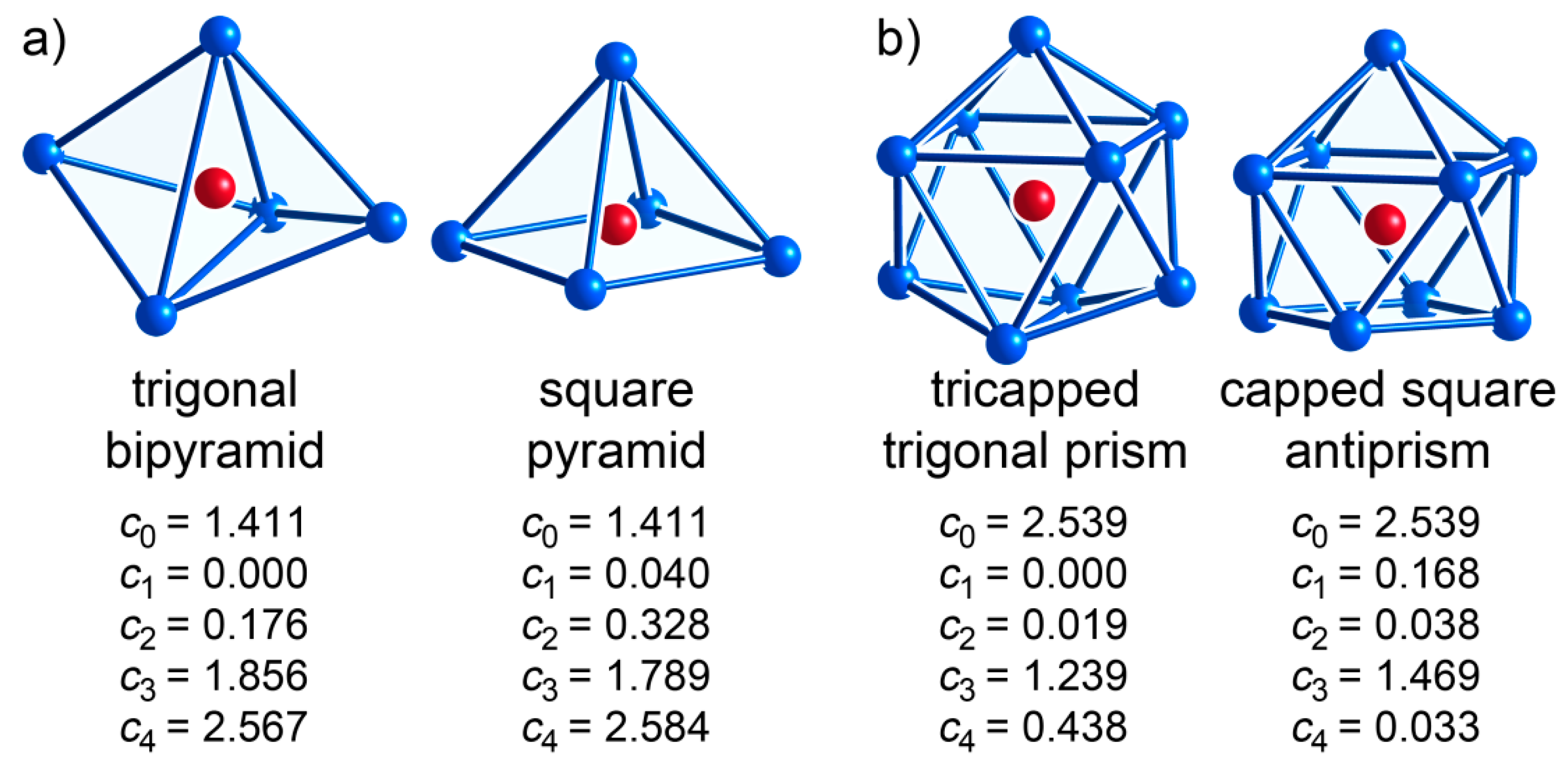
This function is then expanded into an orthonormal basis of real-valued functions on the unit sphere, the real spherical harmonics (SHs). The result of this expansion is a set of vectors of SH coefficients { v l } corresponding to each l value: v 0 = r s , v 1 = ( r p x , r p y , r p z ) , v 2 = ( r d z 2 , r d x 2 y 2 , r d x y , r d x z , r d y z ) , etc. This expansion is then truncated up to an arbitrary order. In the current algorithm, l max = 4 , i.e., only the s, p, d, f and g components are considered. Including higher order coefficients may enhance the level of detail treated in the algorithm at the expense of longer execution time. The program then proceeds to compute the total norm of SH coefficients corresponding to each l value, i.e., c l = | v l | . Since these norms are isometry invariant, they collectively serve as a descriptor of the CE.
(4)
Finally, the distance between two CEs can be calculated as d ( C E 1 , C E 2 ) = l = 0 l max 1 2 l + 1 | c l 1 c l 2 | , where ( c 0 i , c 1 i , c 2 i , , c l max i ) with i = 1 , 2 are the descriptors of the two CEs. The factors 1 2 l + 1 are used to normalize all terms in the summation to the same scale, since v l has 2 l + 1 components.
From the algorithm described above, it can be seen that information loss occurs at two steps: when the SH series is truncated at l max , and when the vector norm for each l is computed. Therefore, having the same set of descriptors does not absolutely guarantee the CEs to be identical. However, from our experience, this information loss is nonessential when l max = 4 is used, as can be rationalized by the fact that certain geometrical constraints will apply to the atomic positions of a realistic CE.
As can be seen from the descriptor data calculated for common CE polyhedra (Table 1), different CEs generally have distinct descriptor values. In the cases where the values are similar, there is also geometrical similarity between the corresponding polyhedra, such as the trigonal bipyramid and square pyramid (Figure 1a) and the tricapped trigonal prism and capped square antiprism (Figure 1b). In other words, the descriptors (with l max = 4 ) indeed serve the purpose of determining similarities and differences between CEs.

2.2. Comparing Multi-Element CEs

For structures containing several elements, each CE may contain atoms of multiple elements. Capturing the elemental identity of atoms within a CE requires some further development of the algorithm. First, when structures contain atoms of different sizes, the Voronoi–Dirichlet scheme of partitioning space between atoms with equidistant planes becomes less justifiable. When a large atom is in contact with a smaller one, it makes more sense to draw the boundary between them closer to the smaller atom.
The power diagram (PD) is a generalization of the Voronoi–Dirichlet diagram that allows us to make such modifications, as has been explored previously by Fischer and coworkers under the name of “radical planes” [56]. Here, each atomic position p i is associated with a radius r i , which in our case corresponds to the atomic radius, and the interface between two PD cells i and j is composed of those points p that satisfy | p p i | 2 r i 2 = | p p j | 2 r j 2 . From this definition, it can be seen that points with larger radii tend to occupy more space as expected, and that the power diagram is reduced to the Voronoi–Dirichlet diagram when all radii assigned are equal. Using a power diagram instead of a Voronoi–Dirichlet diagram places greater emphasis on contacts between larger atoms for any given distance (in the case of Ce-Ni-Si system, the Ce-Ce contacts), in line with chemical intuition.
With the CEs thus defined, we can move on to finding a set of descriptors for the multi-element CE. The straightforward approach is to visualize it as a union of interpenetrating CEs each containing only one element type (we will refer to these units as elemental CEs). However, a simple collection of the descriptors corresponding to each elemental CE is not enough to describe the total CE for several reasons: First, the relative alignment between elemental CEs matters. Keeping one elemental CE fixed while rotating another would result in very different total CEs. Second, the degree of chemical similarity varies between different pairs of elements. As is mentioned at the beginning of Section 2, site substitution by a chemically similar atom should result in smaller changes to the descriptors than by a chemically distinct atom.
PRINCEPS solves the first issue by utilizing what we call the cross-element matrices for each l. For each l, if we collect the l-th order SH coefficients for the i-th elemental CE into a row vector called v l ( i ) , then the cross-element matrix is an N el × N el matrix C l ( N el = number of elements in the system) whose elements are defined as C l , i j = v l ( i ) · v l ( j ) , the inner product of two such vectors. This can be rewritten as C l = S l · S l T , where S l = def ( v l ( 1 ) v l ( N el ) ) is the matrix collecting the l-th order SH coefficient vectors for all elements. The matrix elements along the diagonal of this matrix thus correspond to the squares of the l-th order descriptors of the corresponding elemental CEs, and the off-diagonal terms provide information about the relative orientations of the elemental CEs. In other words, the descriptor of a multi-element CE is not a ( l max + 1 )-dimensional vector, but a N el × N el × ( l max + 1 ) 3D-matrix. This new set of descriptors takes relative orientation between elemental CEs into account, hence solving the first issue listed above.
Concerning the issue of the chemical distinctness of different elements, our initial attempt to account for chemical similarities involved using the Mendeleev number. The Mendeleev number ( R M ) is an alternative way of numbering elements in the periodic table, which sorts them by their chemical properties rather than by number of protons in their nuclei [57]. For example, electropositive metals (such as alkali and alkaline-earth metals) have small Mendeleev numbers, while non-metals have large ones. Incorporation of Mendeleev numbers into the PRINCEPS algorithm in principle would allow us to account for the chemical properties of the elements. However, different Mendeleev numbers do not provide an even scale of chemical similarity between different elements. For example, Sc ( R M = 19 ) and Ti ( R M = 51 ) are normally considered to be more chemically similar to each other than Ti ( R M = 51 ) and Cu ( R M = 72 ), but the difference in Mendeleev number for the former pair is larger than for the latter one (32 vs. 21).
In considering what might be a suitable substitute for the Mendeleev numbers, we found that a simple ratio of an element’s electronegativity and atomic radius is surprisingly effective at sorting elements according to their chemical similarity. As can be seen in Figure 2, where we have tabulated this chemical index ( C I = E N r ), p-block elements above the metal/non-metal line have CI values near two or higher, while the transition metal and metalloid elements fall in the range of 0.8 and 1.8. Finally the electropositive alkali, alkaline earth, and rare earth metals tend to have values below 0.85.
Of course, there are numerous ways we can envision to metricize the similarity between elements. The simple ratio between electronegativity and atomic radius, as is adopted in this Article, works well in terms of sorting metallic elements according to their similar atomic properties. On the other hand, it is possible that when combining a more diverse set of elements, more sophisticated schemes could be used. One feasible alternative of defining chemical similarity is through the utilization of the Darken–Gurry maps (as suggested by one of the reviewers of this work), an empirical rule of predicting the solubility of one element in another, in which the electronegativies and atomic sizes of two elements are compared separately [58]. The PRINCEPS algorithm can be easily adapted to different definitions of the CI.
Once the CI values are calculated, they are incorporated into the algorithm through what we call recombination matrices. After the SH coefficients of the elemental CEs are calculated, they are multiplied by the recombination matrix to allow SH components of different elements to mix:
S l , new = R · S l
where R is the N el × N el recombination matrix and S l is the N el × ( l + 1 ) matrix containing the l-th order SH coefficients of all elements.
The elements in the R matrix are all in the range of 0 R i j 1 . An off-diagonal term of 1 means complete mixing of the two elements, and 0 means no mixing. The R matrix is obtained in a two-step process. First, we compute an auxiliary matrix R sym as:
R sym , i j = C I 0 | C I i C I j | + C I 0
where C I 0 is an arbitrary parameter that controls the differentiation between elements. When C I 0 = 0 , all elements are considered completely distinct (no mixing), and C I 0 = considers all elements to be identical (complete mixing).
Figure 3 illustrates the effect of varying the C I 0 parameter, where three pairs of elements are shown to represent some typical values for Δ C I . For the smallest C I 0 values, the mixing between elements falls steeply as their difference in chemical index increases, while larger C I 0 values leads to more substantial mixing. For intermetallics, we have found C I 0 = 0.1 works well for most intermetallic systems, since it provides strong differentiation between chemically distinct metallic elements (e.g., Ca and Tl), but still allows for a reasonable degree of mixing between chemically similar atoms (e.g., Fe and Co). The user could also tune the extent of mixing between elements through this parameter, which adds to the flexibility of the algorithm.
The R sym matrix thus constructed contains the desired map of similarities among the elements of a system. However, using it on its own would simply blur the identities of the elements, without keeping track of their differences. To correct for this, we perform a Cholesky decomposition on R sym : R sym = R T R , where R is an upper triangular matrix. The use of R rather than R sym allows for a more informative mapping of chemical similarities and differences of the elements.
Let us see how this works with a specific example. In the Ce-Ni-Si ternary system, Ni and Si have similar radii and electronegativities, and Ni/Si mixed sites are very common in the Ce-Ni-Si system, while Ce is more distinct from the other two elements. Calculation of chemical indices yields C I Ce = 1.22 1.80 = 0.68 , C I Ni = 1.91 1.24 = 1.54 , and C I Si = 1.90 1.25 = 1.52 . Setting C I 0 = 0.1 as described above, we have
R sym = ( 1 0.10 0.11 0.10 1 0.99 0.11 0.99 1 ) , R = ( 1 0.10 0.11 0 0.99 0.99 0 0 0.09 )
Now the recombination S l , new = R · S l can be rewritten as:
( Ce new Ni new Si new ) = ( 1 0.10 0.11 0 0.99 0.99 0 0 0.09 ) ( Ce Ni Si )
where Ce , Ce new , etc. represent row vectors of SH coefficients of the l-th order.
From the first row, we have Ce new = Ce + 0.10 Ni + 0.11 Si , i.e., Ce gets very little mixing from Ni and Si, since it is chemically distinct from the other elements. In the second row, the remainder of the coefficients are recombined, and we have Ni new = 0.99 Ni + 0.99 Si , an almost complete mixing of Si into Ni since they are chemically similar. Finally, there is a small Si component in the third row corresponding to the ways in which Si is different from Ce and Ni: Si new = 0.09 Si .
As can be observed from this example, the Cholesky decomposition separates the similarity and distinction between two elements into different rows. For example, Ni and Si are considered chemically similar in the Ce-Ni-Si system, which is accounted for in the mixing in the second row ( Ni new = 0.99 Ni + 0.99 Si ). On the other hand, their distinction, despite being small, still needs to be taken into account. This is accomplished in the mixing of the third row ( Si new = 0.09 Si ), where we have filtered out their similarity and only the distinction is retained.
One issue that needs to be addressed is that the Cholesky projection depends on the order of the elements listed in R sym (e.g., Ce-Ni-Si or Si-Ni-Ce). Changing the order of the elements will also affect the final distance (though the difference is normally insignificant). To completely eliminate this dependency, the algorithm for calculating the distance between CEs loops through all possible permutations of the elements and averages over the distances calculated for each permutation.
In the actual program, PRINCEPS first calculates the cross-element matrices C l of the unmixed elemental CEs, then multiplies them by R and R T on both sides inside the loop over permutations of the elements. As C l , new = S l , new · S l , new T = R · S l · S l T · R T = R · C l · R T , this calculation is mathematically equivalent to the procedure we described above, but is more computationally efficient.
Overall, the PRINCEPS distance between two multi-element CEs (defined in the abstract descriptor space) is then calculated through the following procedure:
(1)
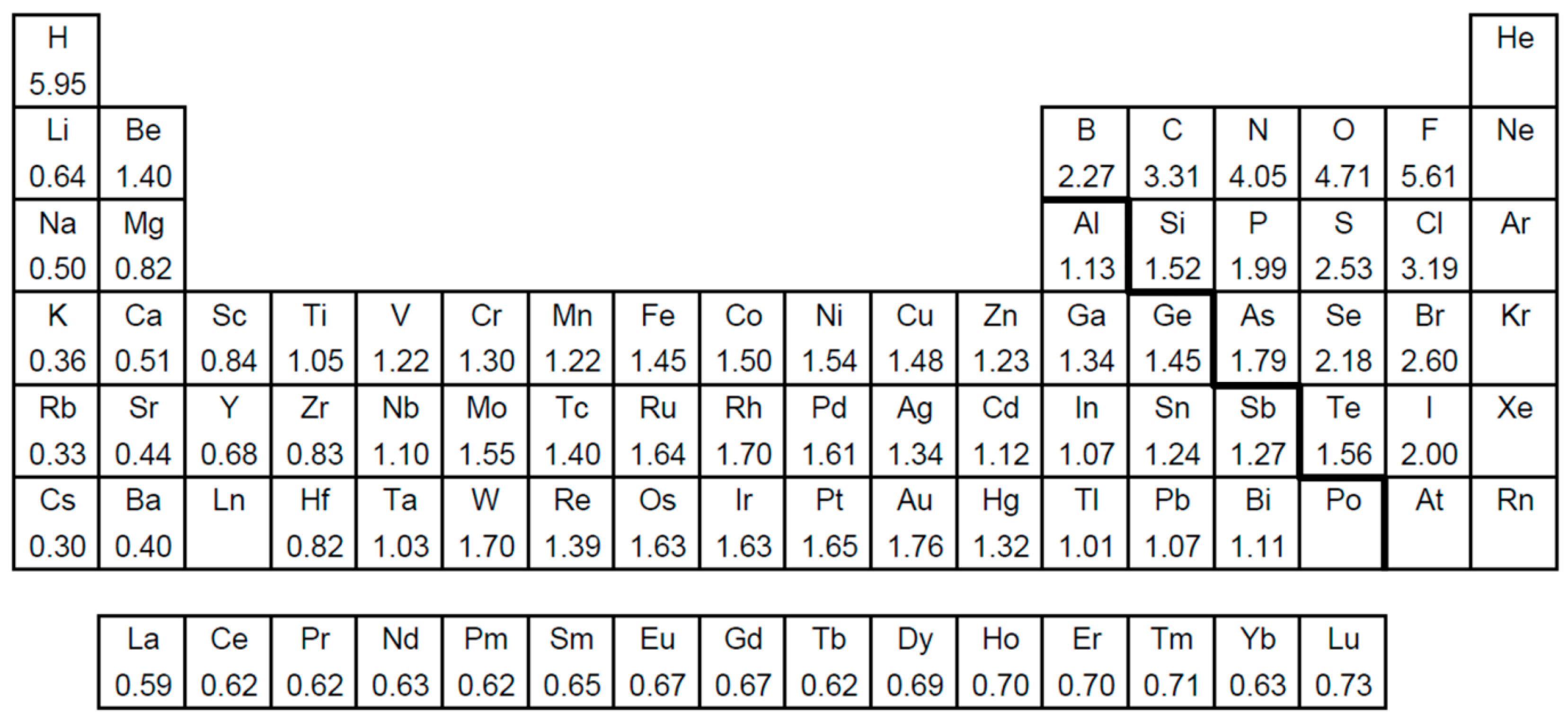
The CE is determined through a power diagram partition of the space using atomic radii.
(2)
Each atom in the total CE is assigned a weight equal to the solid angle of the shared PD face, normalized by the average over all atoms in CE. We thus obtain a function defined on the unit sphere around the central atom for each elemental CE.
(3)
The function for each elemental CE is then expanded into real SHs and truncated up to l max , and the coefficients are collected in l max + 1 matrices S 0 , , S l max .
(4)
( l max + 1 ) cross-element matrices C l are calculated from the coefficients by C l = S l · S l T . The resulting N el × N el × ( l max + 1 ) 3D-matrix is the descriptor of the total CE.
(5)
Determination of the distance between two CEs involves a loop over all possible permutations of the elements:
(5a)
For each permutation σ , the symmetric recombination matrix R sym , σ is calculated, and the recombination matrix R σ is calculated by performing a Cholesky decomposition on R sym , σ .
(5b)
For each l = 0 , 1 , l max , the distance of the two CEs under permutation σ is calculated by d l σ ( CE 1 , CE 2 ) = || R σ · ( C l 1 C l 2 ) · R σ T || , where C l i is the l-th order cross-element matrix of the descriptor of CE i   ( i = 1 , 2 ) , with rows and columns permuted according to σ . || · || denotes the standard matrix norm.
(5c)
The distance between the two CEs under permutation σ is defined as d σ ( CE 1 , CE 2 ) = l = 0 l max 1 2 l + 1 d l σ ( CE 1 , CE 2 ) , where 1 2 l + 1 is the normalization factor for d l σ .
(6)
The overall distance between the two CEs d ( CE 1 , CE 2 ) is then calculated by taking the average of d σ ( CE 1 , CE 2 ) over all permutations σ .
The algorithm so far does not take the identity of the central atom into account. An additional term d central is added to the distance to include this factor: d central ( CE 1 , CE 2 ) = Δ o T · R sym · Δ o , where Δ o = o 1 o 2 is the difference between the occupancy vectors (column vectors whose N el components are the fractional occupancies of the elements on the sites) of the two sites to be compared. Here, the incorporation of the R sym matrix in the calculation allows chemical similarity to be taken into account in comparing sites occupied by atoms of different elements.

2.3. From CEs to Structures

The above procedure provides a comparison between two different CEs. How can this be extended to comparing whole crystal structures? A simple way to start is to calculate distances between each pair of symmetry inequivalent sites using the algorithm described above, creating a p × q matrix where p and q are the number of inequivalent sites in the two structures, respectively. After this matrix is constructed, each site in structure 1 can be paired with the site in structure 2 that bears highest resemblance to it by finding the smallest element along that row in the PRINCEPS distance matrix. These shortest distances together measure to what extent fragments of structure 1 can be considered as structural components of structure 2.
Before combining these shortest distances to get the overall distance between the two structures, they need to go through an additional normalization process, due to the fact that the magnitude of the PRINCEPS distance between larger atoms’ CEs are usually higher. This is because larger atoms normally have more neighbors in their CEs, since the number of atoms in a CE generally scales with the surface area of the coordination sphere ( r 2 ). To counteract this effect, as the shortest distance in each row in the PRINCEPS distance matrix (which contains distances between a given site in structure 1 to all sites in structure 2) is selected, it is divided by the square of the radius of the central atom [59].
Incorporating this factor, the multiplicity-weighted average of the shortest distances of all sites in structure 1 to sites in structure 2 can be calculated. A similar value can be calculated by finding the shortest distance for each site in structure 2 to all of the sites in structure 1 (as is found by scanning the columns of the PRINCEPS distance matrix), and then taking the weighted average of the shortest distances obtained for the sites of structure 2. The overall distance between structures 1 and 2 is then defined as the smaller of these two values to ensure the distance is symmetrically defined.

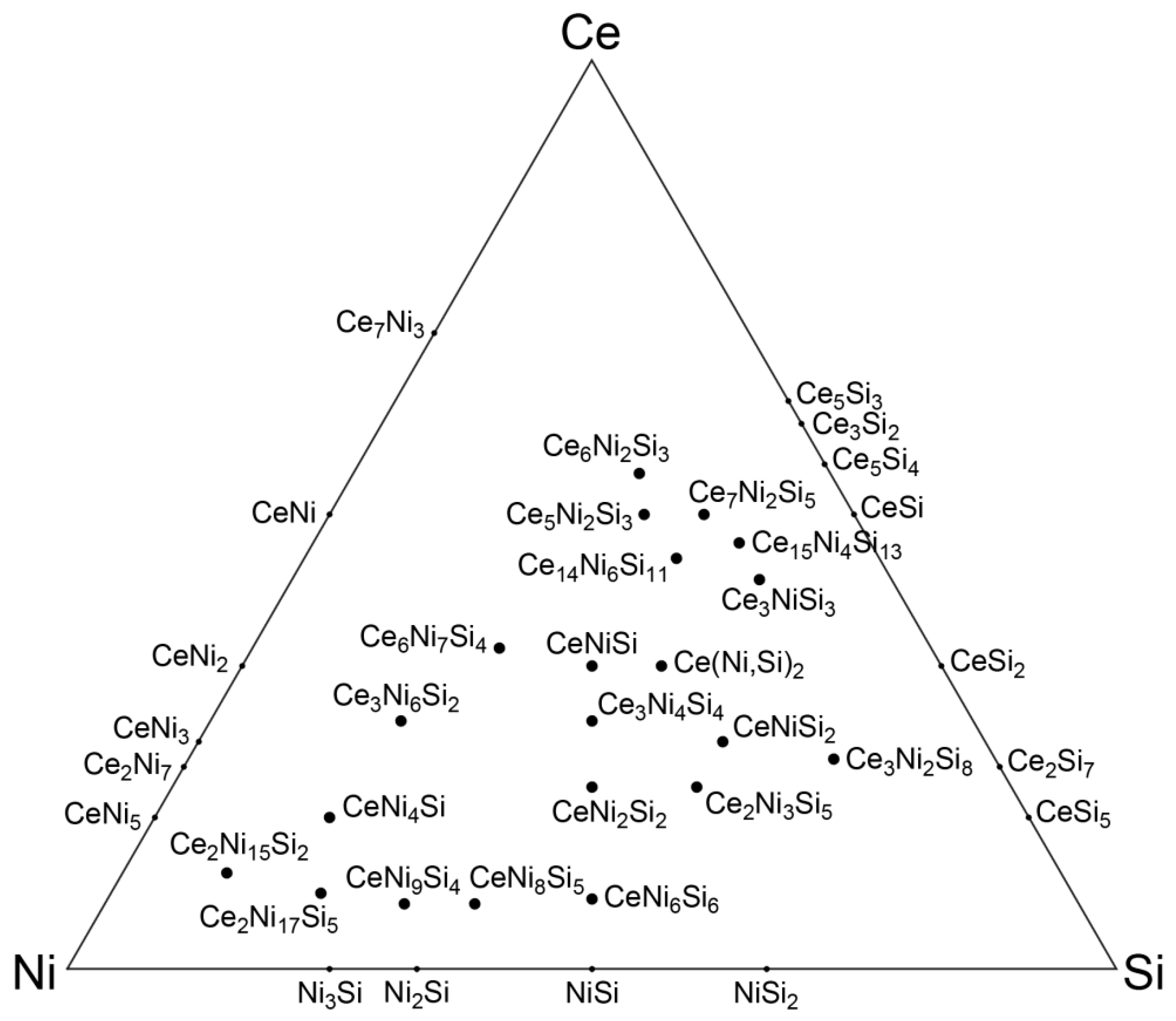
3. Analysis of Crystal Structures in the Ce-Ni-Si System

In this section, we will demonstrate how the above algorithm, as implemented in the PRINCEPS package, can be used in the rationalization of crystal structures in an exceptionally complex system: the Ce-Ni-Si ternary phase diagram (Figure 4) with 17 binary phases and 21 ternary phases. Many of the crystal structures of this system are well-described in the literature [60,61], which reveals rich interrelationships among its structures. In the following sections, we will see how PRINCEPS uncovers these patterns interconnecting the phase diagram’s seemingly chaotic scattering of phases, with minimal intervention on the part of the user. In this analysis, PRINCEPS will interpret the structural motifs of each complex ternary phase in terms of the simpler binary phases in the system, and recognize structural families based on common geometrical motifs.

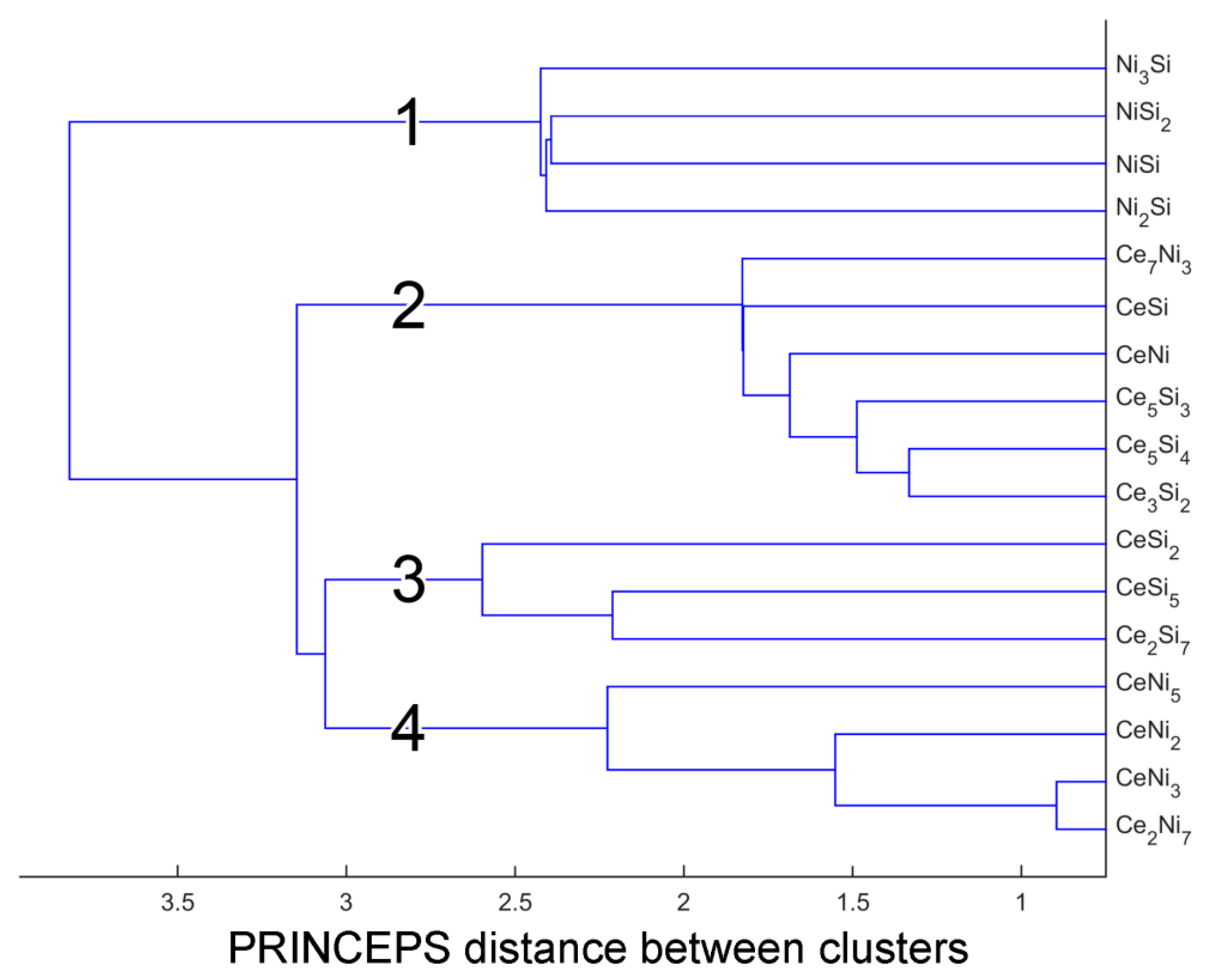
3.1. Defining the Reference Database: Elimination of Redundant Structures

In our analysis, one goal is to project fragments of a complex structure onto simple structure types, much as a wave function in quantum mechanics is projected onto a basis set. As in quantum chemistry, the basis vectors need to be orthogonalized to the greatest extent possible to obtain an effective and unambiguous decomposition, i.e., redundant reference structures that are themselves variants or intergrowths of other reference structures need to be eliminated to ensure a good projection quality. This process thus serves the purpose of removing complicated binary phases (which could possibly be derived from simpler binary phases, e.g., Ce2Ni7 and CeNi3 are intergrowths of CeNi5 and CeNi2), and leaving only the most simple and common structure types in the reference set, which are more commonly used in structural descriptions.
This elimination process can be accomplished by generating a distance matrix between all phases to be analyzed, and applying the standard nearest neighbor clustering algorithm. Near structural duplicates in the reference phases can then be identified by their clustering in the results of the analysis, as can be displayed with a similarity dendrogram (Figure 5).
Applying such a clustering analysis on all binary phases [63,64,65,66,67,68,69,70,71,72,73,74,75,76,77,78,79,80] in the Ce-Ni-Si system yields four clusters:
Cluster 1:Ni2Si ( oP12, P b n m ), Ni3Si (cP4, P m 3 ¯ m ), NiSi (oP8, P n m a ), NiSi2 (cF12, F m 3 ¯ m )
Cluster 2:Ce3Si2 (tP10, P 4 / m b m ), Ce5Si3 (tI32, I 4 / m c m ), Ce5Si4 (tP36, P 4 1 2 1 2 ), Ce7Ni3 (hP20, P 6 3 m c ), CeNi (oS8, C m c m ), CeSi (oP8, P n m a )
Cluster 3:Ce2Si7 (oS18, C m m m ), CeSi2 (tI12, I 4 1 / a m d ) [81], CeSi5 (oI12, I m m m )
Cluster 4:Ce2Ni7 (hP36, P 6 3 / m m c ), CeNi2 (cF24, F d 3 ¯ m ), CeNi3 (hP24, P 6 3 / m m c ), CeNi5 (hP6, P 6 / m m m )
In principle, only one representative should be needed from each cluster to capture the geometrical features the phase within the cluster represent, particularly when the structures are connected by substructure-superstructure relationships. It is reasonable to choose the simplest structure from each cluster, i.e., the structure with fewest atoms in each unit cell, as the representative. Therefore, Ni3Si (cP4), CeSi (oP8), CeSi2 (tI12) and CeNi5 (hP6) are chosen as reference phases in our analysis.
In addition to these four binary phases, we also added two ternary phases, Ce(Ni,Si)2 (AlB2-type, hP3) [82] and CeNi2Si2 (ThCr2Si2-type, tI10) [83], because they both adopt simple and common structure types that are not represented in the binary phases. The MgCu2 type structure of CeNi2 (cF24) previously removed from the list due to its similarity to CeNi5 also fits this criterion of being common and simple (though its unit cell is significantly larger than those of any of the other reference structures), but its inclusion was not found to significantly influence the PRINCEPS results. Altogether then, we will interpret the ternary structures within the Ce-Ni-Si system with a collection of six reference structures: their basic crystallographic information is listed in Table 2, while the distance matrix for these phases is tabulated in Table 3.
From Table 3, it can be seen that all reference phases we selected differ significantly from each other, with the exception of the pair Ce(Ni,Si)2 and CeSi2. As will be further elucidated in the following sections, these two structures have similar local CEs, but very distinct long-range topologies: as a result, we will be keeping both structures in our reference library for the subsequent analyses.

3.2. Projection of Ternary Phases onto Simple Binary Phases: Sample Output

Having identified a set of reference phases for the Ce-Ni-Si system, we now examine how the more complex structures in the system can be interpreted in terms of this reference set. For now, we will focus on five ternary phases chosen to illustrate the different types of results that may arise from a PRINCEPS analysis. Let us begin by looking at the information PRINCEPS provides in its output, an example of which is shown in Figure 6. In later sections, this information will be summarized in tables for clarity.
In this output, the program goes site-by-site through the phase analyzed, and annotates each site label with three numbers in parentheses giving the number of atoms of each element type in its CE (the site’s coordination vector). For example, Ce1 in CeNiSi2 has 6 Ce, 5 Ni and 10 Si atoms in its CE. These numbers can be fractional, which indicates mixed occupancy of certain sites in the structure. A site “Mx1” can also be found in the output, which corresponds to the mixed occupancy site Ni1/Si1 in Ce(Ni,Si)2 (the CeNiSi# structure in the output).
Following the coordination vector is the site’s projection quality. This value is determined by the shortest distance of that site’s CE to those of the sites in the reference collection (a distance of zero would correspond to a quality of 100%), and is also dependent on the element type: a larger atom (such as Ce) has more atoms in its CE, so its PRINCEPS-distances to other Ce sites’ CEs tend to have larger values.
Next comes a list of the three sites in the reference collection with the shortest CE distances to the site in question, along with their coordination vectors. After the site-by-site listing, a summary is given. Based on the distances of each atom to the sites in the reference phases, the fraction of the structure’s atoms belonging to each reference structure is listed. The summary also gives an overall decomposition quality, calculated from the site-wise projection qualities. Specific formulae for the calculation of the projection quality, overall decomposition quality, and decomposition weight are given in the Supporting Information.

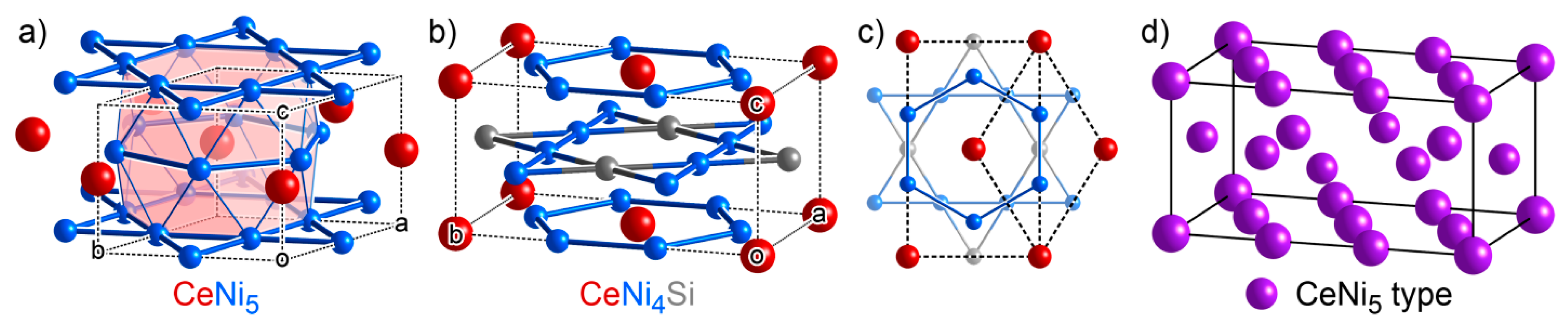
3.3. CeNi4Si: An Ordered Ternary Variant of a Binary Structure

Now that we have covered the core PRINCEPS output, we are in a position to use this approach to bring structural insights into complex systems, such as the Ce-Ni-Si phase diagram. Let us start with a simple case, CeNi4Si (oS12, C m m m ) [85]. As can be seen in the PRINCEPS output summarized in Table 4, all four sites in CeNi4Si finds their best matches in the reference phase CeNi5, with high projection qualities (higher than 80% for all sites, 99% for Ce1). This also results in an overall decomposition weight of nearly 100% on CeNi5, and a very high decomposition quality of 91.64%. The combination of one predominant decomposition component and high decomposition quality is the typical result for a ternary variant of a binary or elemental reference phase.
These features are immediately evident when comparing the crystal structure of CeNi4Si to that of CeNi5 (Figure 7). CeNi5 adopts the CaCu5 structure type (Figure 7a), in which alternating layers of honeycomb and kagome nets of Ni as well as hexagonal voids occupied by Ce atoms can be identified. In CeNi4Si (Figure 7b), the same stacking pattern of the alternating nets can be perceived, confirming that it is indeed a ternary variant of CeNi5. The essential difference from the binary phase is that some Ni atoms in the kagome net are replaced by Si atoms, which lowers the space group symmetry from P 6 / m m m to C m m m , with the unit cell of CeNi4Si then being the C-centered orthorhombic supercell of the hexagonal cell of CeNi5 (Figure 7c).
To help visualize this relationship, PRINCEPS also automatically generates a color-coded site projection map (Figure 7d). In this figure, a color is assigned to each reference phase, rather than each element type. The color of each atom in the unit cell then represents the reference phase it is assigned to (i.e., the reference phase that contains the site that best matches the target atom), while the size of that atom reflects its projection quality. For CeNi4Si, where all sites in the structure are highly similar to CeNi5, the figure shows exclusively purple atoms, the color assigned to CeNi5. The spheres also have large radii (relative to others we will see below), indicating good projection quality into CeNi5 throughout the unit cell. Note that while large spheres in a projection map indicate a high resemblance to the reference phase, small spheres (i.e., poor fitting) could be due to several reasons, such as distortions or missing atoms. Efforts to more deeply understand the crystal structure in question can then be focused on these sites of low projection quality.

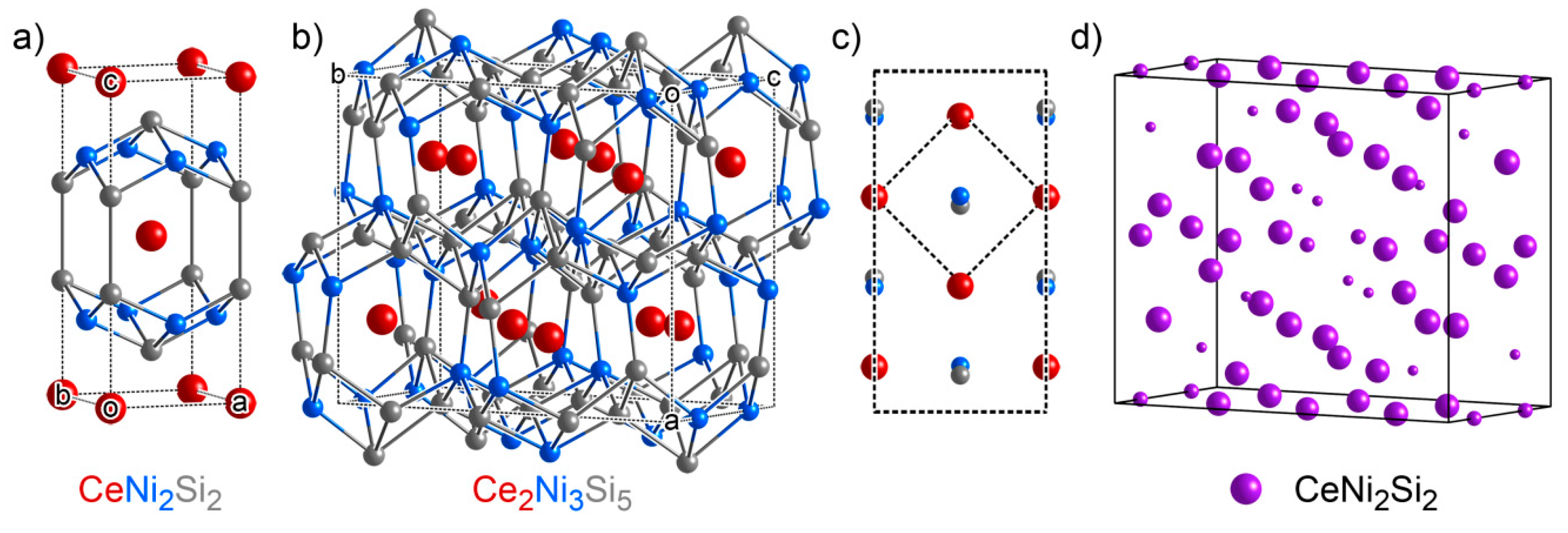
3.4. Ce2Ni3Si5: Another Ternary Variant Structure

The structure of Ce2Ni3Si5 (oI40, I b a m ) offers the opportunity to explore a slightly more complicated example of a ternary variant of a binary structure type [86]. The output of PRINCEPS analysis for this phase (Table 5) shows projection qualities significantly lower than those for CeNi4Si: most sites have a projection quality ranging between 60% and 80%, and the overall quality is only 63.12%, compared to 91.64% for CeNi4Si. However, for each site, the reference phase that gives the best match is unequivocally CeNi2Si2, which also dominates the overall decomposition, with a weight of 80.69%. Therefore, despite the lower decomposition quality, this result still hints that Ce2Ni3Si5 is closely related to CeNi2Si2, but with distortions obscuring the relationship.
A closer look at the crystal structures confirms this hypothesis (Figure 8). CeNi2Si2 adopts the common ThCr2Si2 structure type (Figure 8a), in which stacked sheets of edge-sharing Ni@Si4 tetrahedra provide large cavities for the placement of Ce atoms. In Ce2Ni3Si5, a similar Ni/Si framework hosting Ce atoms is apparent, but the arrangement of Ni and Si atoms is different, and it is quite distorted relative to the framework in CeNi2Si2 (Figure 8b). These changes lead to Ce2Ni3Si5 being a supercell variant of CeNi2Si2 (Figure 8c). The distortions alter the weights of the coordinating atoms in the descriptors of the CEs, and in some cases (such as Ce1) completely eliminate an atom from a CE (Ce1 has a coordination number of 21 in Ce2Ni3Si5, compared to 22 in CeNi2Si2).
In the site projection map generated by PRINCEPS (Figure 8d), it is also clear that although the structure still shows exclusively purple atoms (the color assigned to CeNi2Si2), some sites are not very well reproduced by this reference phase, as is indicated by the relatively small radii of the spheres on these atoms.

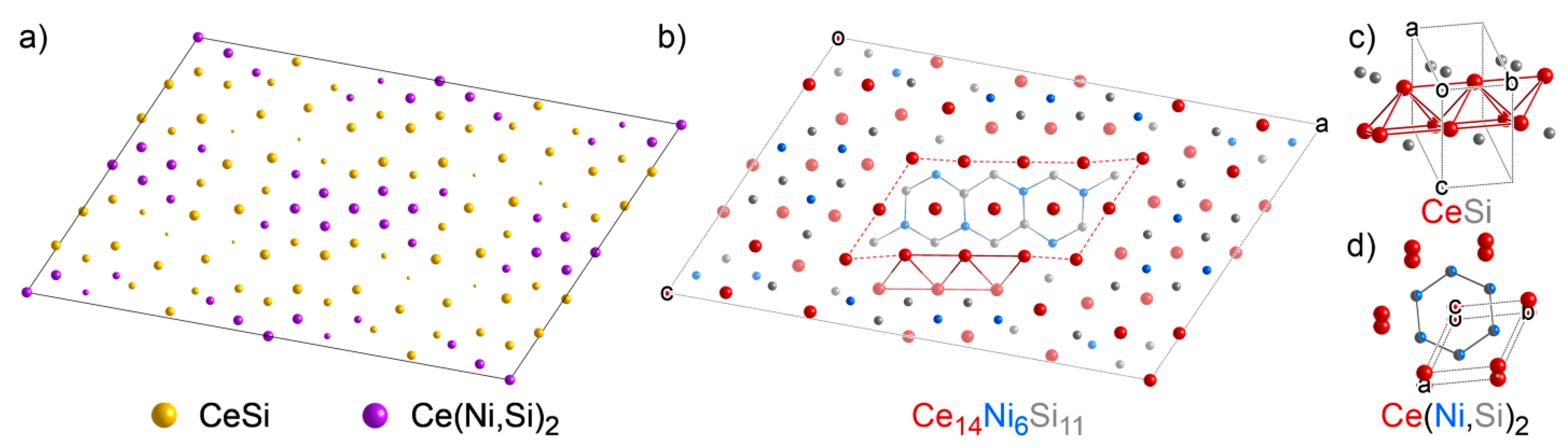
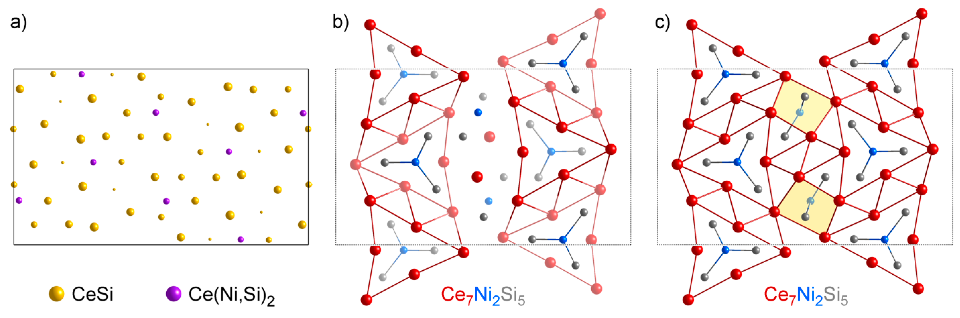
3.5. Ce14Ni6Si11: An Intergrowth of Reference Structures

In the previous two examples, we have demonstrated how PRINCEPS identifies connections between structures that follow simple superstructure variants of a reference phase, even with a significant amount of distortion. In this section, we move up in complexity to a case in which a single reference phase is no longer sufficient: Ce14Ni6Si11 (mC124, C 2 / m ) [87]. The inadequacy of a single reference phase for the description of this structure is evident immediately in the PRINCEPS output, shown for selected sites in Table 6.
The projection qualities for most sites are above 80%, indicating that the library of reference phases does well in characterizing this structure. However, unlike the cases we have seen previously, not all sites find their best match in the same reference phase. While a majority of the sites bear the highest resemblance to sites in CeSi (weight = 65.34%), some sites (such as Ce8 and Ni1) are more closely related to the Ce(Ni,Si)2 (weight = 18.70%) and CeSi2 (weight = 15.93%) structures.
A look at the site projection map leads to a simple interpretation of these results. In Figure 9a, we used CeSi and Ce(Ni,Si)2, the two phases with highest decomposition weights, as target phases for the projection. Here, spheres showing the maximum degree of fit to the two phases with the highest weight in the decomposition (CeSi: yellow spheres, Ce(Ni,Si)2: purple spheres) are overlaid on the structure. The large radii for most of the atoms is in accordance with the high projection quality. A more striking feature of this map, however, is the distinct segregation of yellow and purple regions in the unit cell, where the purple atoms highlight small Ce(Ni,Si)2 domains (1D columns that run out of the page) separated by yellow CeSi interfaces. In other words, the PRINCEPS analysis clearly suggests that Ce14Ni6Si11 is an intergrowth of the simpler CeSi and Ce(Ni,Si)2 structure types.
To confirm this structural description, let us look in more detail at the structure of Ce14Ni6Si11. Figure 9b shows the Ce14Ni6Si11 structure, while Figure 9c,d show the structures of the two reference phases, CeSi and Ce(Ni,Si)2, respectively. The red dotted lines highlight a Ce(Ni,Si)2-type domain in the structure, with the Ni/Si atoms connected to show the characteristic hexagonal net found in AlB2-type structures; some Ce atoms next to the Ce(Ni,Si)2 domain are also connected, in order to show the resemblance to the FeB-type CeSi structure. The two domains therefore merge seamlessly along the red dotted line by sharing the Ce atoms on the interface. This description of Ce14Ni6Si11 concurs with the decomposition result given by PRINCEPS, and confirms that it is a complex intergrowth of Ce(Ni,Si)2 and CeSi fragments.
How does the third best-fit reference structure, CeSi2, fit into this story? As we saw earlier in the preparation of our set of reference structures, Ce(Ni,Si)2 and CeSi2 show a high degree of overlap in their local structures, and thus they tend to appear together in the decomposition analysis. Their differences in the long-range structures, however, make having both structures in the set useful. In Ce14Ni6Si11, the Ce(Ni,Si)2 arrangement fits nicely into the structural context of the well-fit sites (Figure 9b), while in other structures CeSi2 provides a better match. This choice is to some extent anticipated by the decomposition weights (18.7% Ce(Ni,Si2) and 15.9% CeSi2 for Ce14Ni6Si11), but becomes quite obvious when attempting to make interpretative pictures of the domains in a complex structure such as that of Figure 9b.

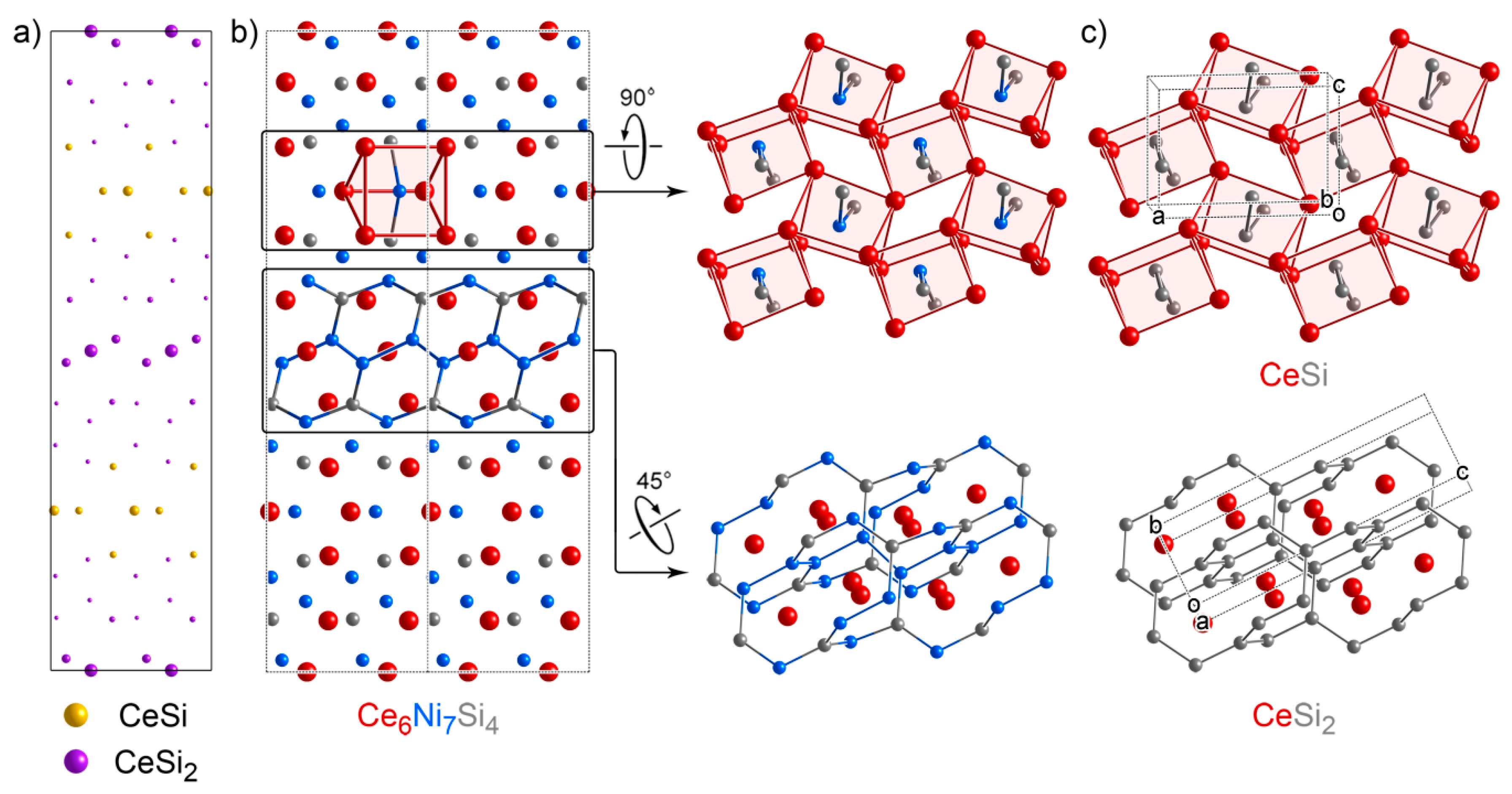
3.6. Ce6Ni7Si4: An Intergrowth with Substantial Relaxation at the Interface

A similar intergrowth scheme can be derived from the PRINCEPS output for Ce6Ni7Si4 (oP68, P b c m ) [62], with some interesting differences (Table 7). As with the results for Ce14Ni6Si11, the PRINCEPS analysis of Ce6Ni7Si4 highlights major contributions from two reference phases, CeSi and CeSi2, which closely represent most sites in the structure. However, the overall decomposition quality is much lower, at a mere 51.91%. While some sites have relatively high projection quality (such as Ce4), some are very poorly reproduced by the reference phases. Due to the low decomposition quality, the answer as to whether Ce6Ni7Si4 can be viewed as an intergrowth of CeSi and CeSi2 appears to be somewhat ambiguous.
The site projection map of Ce6Ni7Si4 (Figure 10a) offers a clearer picture. As is expected from the low decomposition quality, many atoms in the figure have spheres with small radii. However, there is still a clear segregation between CeSi domains and CeSi2 domains, which form 2D layers that stack alternatively along the c axis. The atoms lying at the interior of the layers have spheres with larger radii, while the atoms at the interfaces have smaller ones, suggestive of domains with a high fidelity to a reference structure at the center that is relaxed at the interfaces. The projection map therefore suggests that Ce6Ni7Si4 is a layered intergrowth of CeSi and CeSi2, but instead of these motifs merging seamlessly at the interfaces (as in Ce14Ni6Si11), some compromise has been made at the interfaces that degrade the projection quality.
This analysis opens a path to a detailed structural analysis of Ce6Ni7Si4 (Figure 10b). The slab of atoms associated with the CeSi reference structure (yellow atoms in Figure 10a) is composed of vertex- and edge-sharing Ni@Ce6 trigonal prisms, derived from the CeSi structure. Likewise, the CeSi2 layers (purple atoms in Figure 10a) exhibits the same 3-connected Ni/Si nets found in the CeSi2 structure (ThSi2 structure type). The interface between these layers, however, does not resemble any simple structure type in the Ce-Ni-Si system (it is, in fact, a layer of the TiNiSi type).

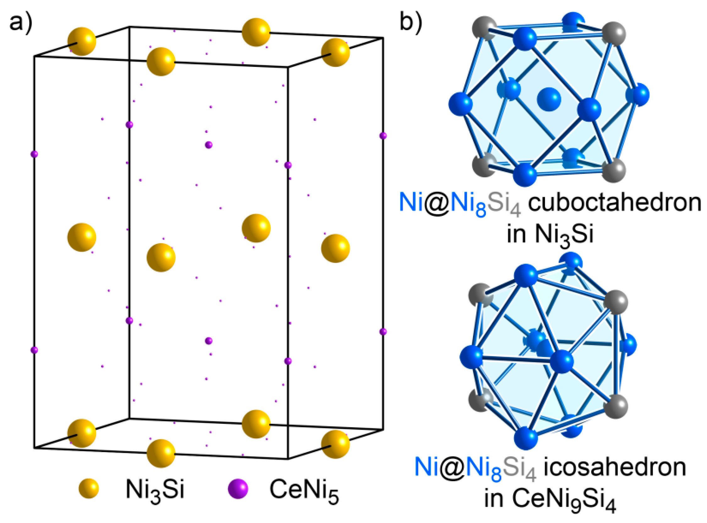
3.7. CeNi9Si4: An Isolated Structure

Now that we have considered examples of structural variants and intergrowths in the Ce-Ni-Si system, let us consider a structure that is not satisfactorily represented by the reference phases, indicating that the compound exhibits structural motifs unique to the ternary phases. We take CeNi9Si4 (tI56, I 4 / m c m ) as the sample structure for this case, whose PRINCEPS analysis is summarized in Table 8 [88].
Compared to the phases discussed above, the overall projection quality is exceptionally low (only 19.79%), indicating that it is not closely related to any of the reference phases. The site projection map of CeNi9Si4 onto Ni3Si (yellow atoms) and CeNi5 (purple atoms), the two reference phases that have the highest weights in the decomposition, is shown in Figure 11a. As can be seen from the figure, despite the fact that these two phases take up a total weight of over 85% in the decomposition, most sites in the CeNi9Si4 unit cell are so poorly reproduced that the spheres on the atoms are hardly visible. At this level of projection quality, the projection weights of the reference phases no longer hold much useful information about the structure of the ternary phase.
The only exception to this general trend is the Ni3 site (large yellow atoms), which has a surprisingly good projection quality of 92.19%. This is due to the similarity of the CE of Ni3, which is an icosahedron, to the CE of Ni atoms in Ni3Si (AuCu3 structure type, a fcc variant), which is a cuboctahedron. When aligned properly it can be seen that these two polyhedra are highly similar (Figure 11b), differing only in rotation of triangular faces of the cuboctahedron, which can only be distinguished by using a l max cutoff higher than 4 [54] (increasing l max in the PRINCEPS analysis could indeed draw a bigger distinction between these two CEs, but at the expense of much longer processing time). The majority of the CeNi9Si4 structure, though, still remains obscure. While this phase does not show strong connections to any binary phases in our reference library, we will see below (in Section 4.5) that it is actually part of a family of ternary phases in this system.

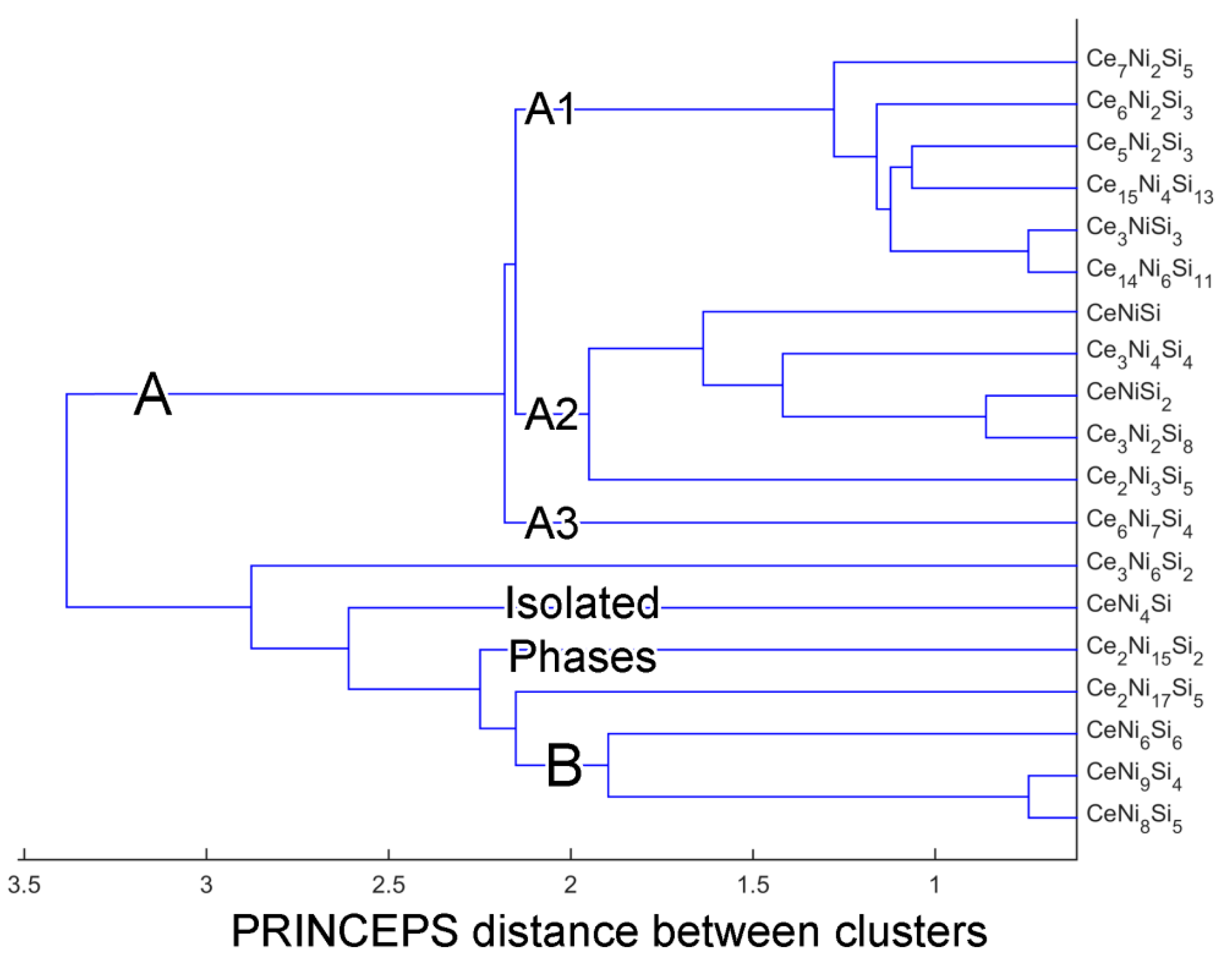
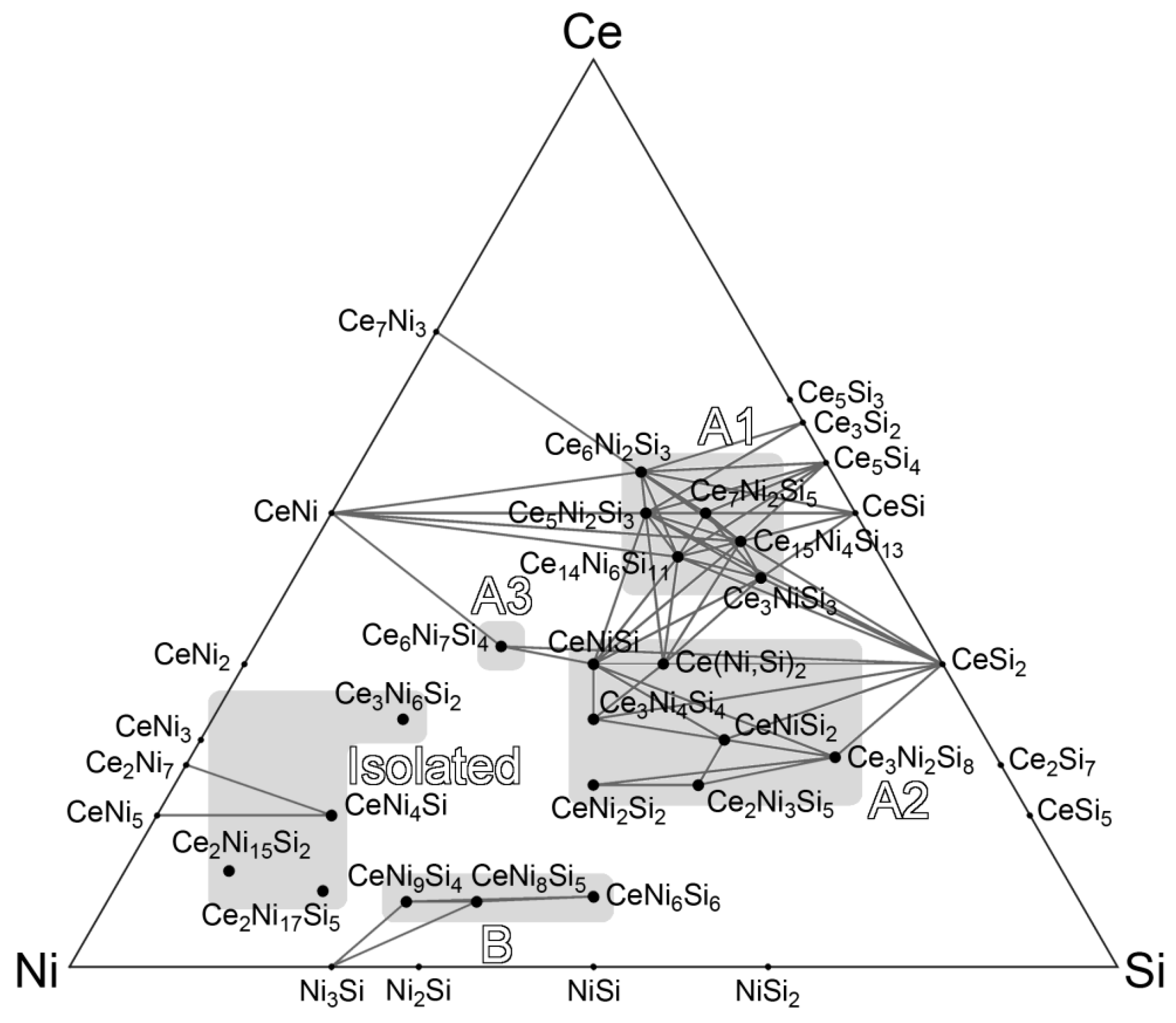
4. Clustering of Ternary Phases and Group-Wise Structural Analysis

In Section 3, we investigated five ternary phases with the help of the PRINCEPS algorithm, categorizing each of them as a variant of a reference phase, an intergrowth of reference phases, or an isolated structure. Through this process, we have seen that PRINCEPS can significantly accelerate the process of structural analysis for such phases. In this section, we will take a further step to categorize the ternary phases into groups by their structural similarity, and identify common structural motifs among the members. We will thus be able to view the phases in the Ce-Ni-Si phase diagram not as individual points, but as connected into structural series, deepening our understanding of this complex ternary system.

4.1. Clustering of Ternary Phases in the Ce-Ni-Si System

As a first attempt to categorize ternary phases, we performed clustering analysis on all ternary phases [62,89,90,91,92,93,94,95,96,97,98,99] in the Ce-Ni-Si system with PRINCEPS. The resulting dendrogram (Figure 12) shows that the ternary phases can be roughly separated into two major branches. In the upper branch, the structures can be divided at the distance of 2.0 into three clusters. Clusters A1 and A2 both contains multiple phases, while cluster A3 consists of just Ce6Ni7Si4. In the lower branch, however, the phases are in general connected more loosely (notice the joining of different branches occurs at much higher distance levels), indicating that weaker structural relationships should be expected. Using a distance cutoff at 2.0 again, it can be observed that the three phases at the bottom form a small cluster (cluster B), while the remaining phases are all disconnected from each other, which we will denote as isolated phases.
While a clustering dendrogram provides some information about structural similarity, it is not detailed enough to show the intricate connections among the phases within each cluster, nor does it show the location of the groups on the phase diagram. To more clearly present the pairwise structural relationships between the ternary phases, PRINCEPS is able to generate ternary phase diagrams connecting phases by their similarities, based on a distance matrix between the phases (Figure 13).
Overall, the connectivity between phases in the phase diagram agrees with the clustering analysis of Figure 12. The six phases located at the upper right correspond to Cluster A1, and are all interconnected with each other, indicating very close structural similarities. Clusters A2 and A3 (Ce6Ni7Si4) are located at the central region. Clusters A1, A2, and A3 are connected to each other through the phase CeNiSi, in accord with the phases being grouped into a common major branch in the cluster analysis. The three phases in cluster B (CeNi9Si4, CeNi8Si5, and CeNi6Si6) form a small connected group, while the isolated phases scatter in the lower left region of the phase diagram and are disconnected from any other ternary compounds.
Combining the results from the clustering analysis and the positions of the compounds in the phase diagram, we can categorize the ternary phases in the Ce-Ni-Si system as listed in Table 9.

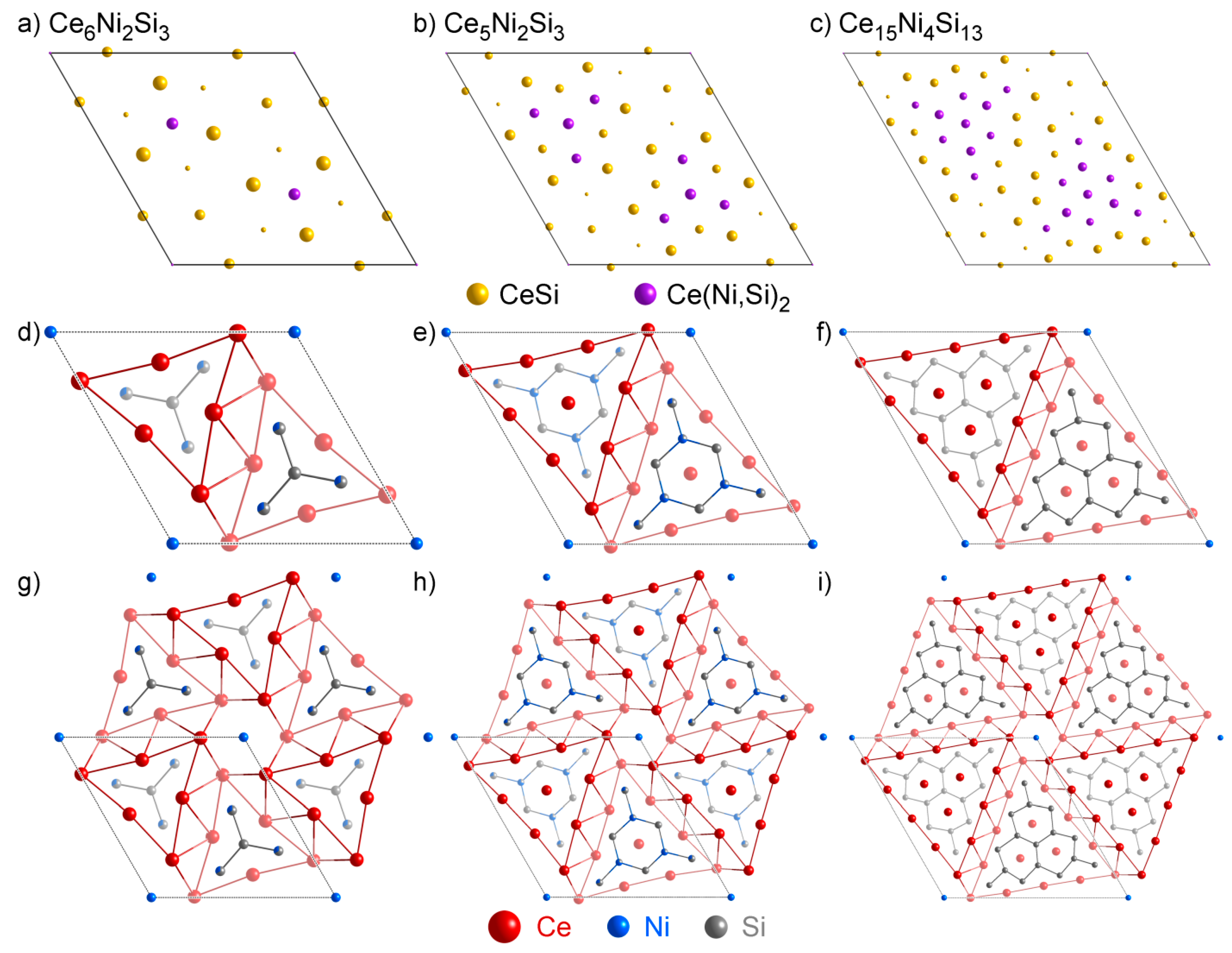
4.2. Analysis of Group A1

As can be seen in the PRINCEPS results summarized in Table 10, the structures of Group A1 are intergrowths of CeSi, Ce(Ni,Si)2, and CeSi2, similar to what we encountered earlier for Ce14Ni6Si11 (Figure 9).
Among these six Group A1 phases, the three structures Ce6Ni2Si3, Ce5Ni2Si3 and Ce15Ni4Si13 are particularly interesting in that they form a clear structural series (Figure 14) [100]. Figure 14a–c shows the site projection map of the three phases onto CeSi (yellow) and Ce(Ni,Si)2 (purple), where a segregation between CeSi and Ce(Ni,Si)2 domains can be found in all three structures, with the size of the Ce(Ni,Si)2 domain gradually increasing across the series. Therefore, all three structures in the series can be explained as intergrowths of the two reference phases. The unit cell structures in the series are shown in Figure 14d–f, which highlights the triangular Ce(Ni,Si)2 domains with increasing sizes, and the CeSi-type interfaces depicted as zigzagging Ce double layers. Figure 14g–i shows larger fragments of these structures, where additional Ni atoms are found to fill up the void where six Ce(Ni,Si)2 triangular domains meet at their shared corners.
As the triangular Ce(Ni,Si)2 domain grows larger, its interior will occupy more space relative to the CeSi interface (in other words, larger bulk size results in a smaller surface to volume ratio). Therefore, when performing the structural decomposition analysis, we would expect the weight on Ce(Ni,Si)2 to increase, and the weight on CeSi to decrease as we go across the series. This trend is indeed observed in Table 10: from Ce6Ni2Si3, Ce5Ni2Si3 to Ce15Ni4Si13, the weight on CeSi gradually decreases from 91.01% to 68.43%, while the weight on Ce(Ni,Si)2 increases from 5.00% to 24.59%.
The Ce7Ni2Si5 presents an alternative way of intergrowing CeSi (yellow) and Ce(Ni,Si)2 (purple) domains (Figure 15a). Again, triangular domains of Ce(Ni,Si)2 are found, which are almost identical to those in Ce6Ni2Si3, both depicted as isolated purple atoms in the site projection map. However, these domains are connected to each other following a different pattern, resulting in chains that run parallel to each other, with some additional atoms filling the void in between. For those Ce(Ni,Si)2-based atoms not at the center of Ce(Ni,Si)2 triangles, Figure 15c reveals their CE to be trigonal prisms, and between them are smaller fragments of the CeSi-type zigzag motif.
The last structure in Group A1, Ce3NiSi3, demonstrates yet another way CeSi and Ce(Ni,Si)2 can intergrow. In its site projection map onto the two reference phases (Figure 16a), the yellow and purple atoms form alternating layers stacking along the c direction. The structure can therefore be described as an intergrowth of CeSi and Ce(Ni,Si)2 slabs (Figure 16b).

4.3. Analysis on Group A2

The structures of Group A2 mark a clear departure from the CeSi-Ce(Ni,Si)2 intergrowths of Group A1. As can be seen in the PRINCEPS output in Table 11, CeSi does not play a significant role in any of these five phases. The first two phases represent structural variants of simple structures: Ce2Ni3Si5 is a variant of CeNi2Si2, as is discussed in Section 3.4. Likewise, CeNiSi is a ternary variant of CeSi2, which is reflected in its high decomposition quality and a high weight for CeSi2 (Figure 17).
The remaining three structures in the group—CeNiSi2, Ce3Ni2Si8 and Ce3Ni4Si4—all have tall pseudo-tetragonal cells (although none of them are actually tetragonal: all three belong to the orthorhombic crystal system). In Figure 18a–c, all three phases are projected onto their major contributing phases, CeNi2Si2 (yellow) and Ce(Ni,Si)2 (purple). From the projection maps, it can be observed that the structures are built from stacking patterns of CeNi2Si2 layers (layer A) and Ce(Ni,Si)2 layers (layer B). Most sites in the three structures exhibit good projection qualities, except those Ce atoms lying on the interface between A- and B-type layers.
Following this projection scheme, all three phases in the series can be viewed as stackings of the A and B layers. The main difference lies in the ordering of the layers. Ce3Ni2Si8 adopts an A-B-A-A-B-A type stacking; in CeNiSi2, the stacking follows the A-B-A-B pattern; in Ce3Ni4Si4, the stacking pattern becomes B-A-B-B-A-B. This trend is in accordance with the decomposition weights listed in Table 11: Ce3Ni2Si8 (A:B = 2:1) has the highest decomposition weight on CeNi2Si2 among the three phases (67.46%), and this number gradually decreases across the series (46.32% for CeNiSi2 with A:B = 1:1, 31.58% for Ce3Ni4Si4 with A:B = 1:2). On the other hand, the decomposition weight on Ce(Ni,Si)2 experiences a steady increase across the series (6.54% for Ce3Ni2Si8, 9.89% for CeNiSi2, 24.87% for Ce3Ni4Si4). The change in decomposition weights of the three phases thus agrees with the trend in the A:B ratio over the structural series.
When examining Table 11, one may notice that the CeSi2 structure is also taking up a large portion of weight in the decompositions. The reason behind this can be seen in Figure 18d: both CeSi2 and Ce(Ni,Si)2 can be viewed as stacking of the B layers. In CeSi2, however, adjacent B layers are related by a 41 screw operation, rather than a simple reflection, so its stacking can be described as B-B’-B-B’. Therefore, in our description of the structural series as stacking of A and B type single layers, CeSi2 and Ce(Ni,Si)2 can be considered as almost equivalent [101,102]. Their difference in relative orientation of adjacent B layers only becomes significant when the target structure also contains adjacent B layers: for example, Ce3Ni4Si4 has weights of 31.58% for Ce(Ni,Si)2 and 24.87% for CeSi2, since its neighboring B layers are related by reflections rather than screw rotations.

4.4. Group A3: The Ce6Ni7Si4 Structure

The structure of Ce6Ni7Si4 has been discussed in Section 3.6. As a special member of Group A, its structure is unique in that it contains CeSi-type layers, a structural motif typical for Group A1, but here they form intergrowths with CeSi2-type layers rather than Ce(Ni,Si)2 fragments, which are more commonly found in Group A2 phases. Therefore, the Ce6Ni7Si4 structure shares some structural features with both Group A1 and Group A2, but does not truly belong to either, explaining why it is listed as a separate cluster by PRINCEPS.

4.5. Analysis on Group B

In our analysis of CeNi9Si4 (Section 3.7), we determined that this phase is not reducible to fragments of the binary phases in the system. As is evident in the PRINCEPS output of Table 12, the same applies to the other members of Group B.
A more productive approach to these compounds is then to examine their relationships with each other, which can be explored through the PRINCEPS distance matrix of Table 13. The distances among these three phases are found to be exceptionally small (for comparison, the average distance between two Ce-Ni-Si ternary phases is 1.90: see the Supporting Information for details), suggesting that high structural similarity may be found between them.
A closer look at the crystal structures confirms this expectation: CeNi8Si5 adopts the NaZn13 structure type (cF112, space group F m 3 ¯ c ). This structure can be rationalized as a CsCl-type packing of Na atoms and Zn@Zn12 filled icosahedra (Figure 19a), with the icosahedra alternatively adopting two different orientations; the Na atoms occupy the void spaces in the Zn sublattice, attaining as their CEs the 24-coordinate polyhedron known as the snub cube. In CeNi8Si5, Ce occupies the Na position, and Ni and Si atoms are mixed on the Zn positions.
The structure of CeNi9Si4 is nearly identical to CeNi8Si5; the only difference is that the Ni and Si atoms are ordered instead of forming mixed occupation sites, lowering the symmetry from cubic ( F m 3 ¯ c ) to tetragonal ( I 4 / m c m ). CeNi6Si6 is another variant, which adopts a different Ni-Si ordering, further lowering the symmetry to P 4 / n b m ; moreover, the central position of the Ni/Si icosahedral cluster is left unoccupied, changing the overall Ce:(Ni + Si) ratio from 1:13 to 1:12.
These features are expressed in the inter-phasic distances of Table 13. CeNi8Si5 and CeNi9Si4 differ chiefly in the ordering of Ni and Si atoms, leading to a distance between them of less than 0.5. The CeNi6Si6 structure, on the other hand, leaves the Ni/Si icosahedra empty, resulting in a more significant change in the atomic CEs and hence a longer distance from the other two phases.

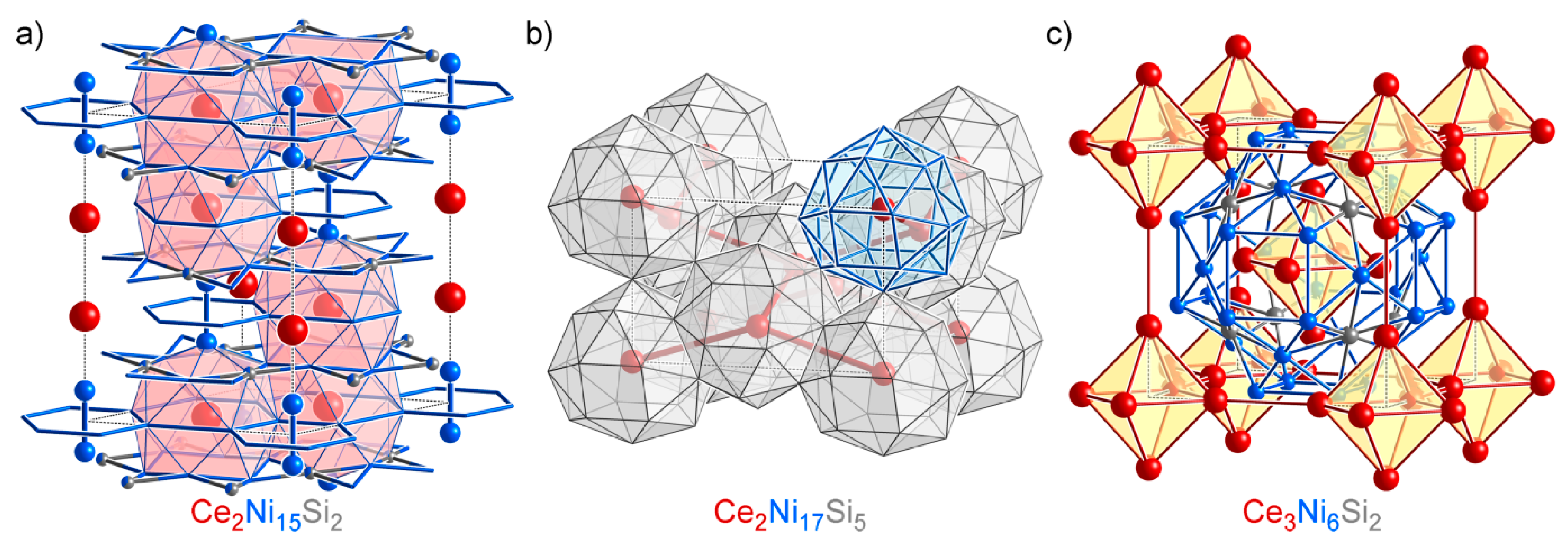
4.6. Overview of the Isolated Phases

As can be seen from the ternary phase diagram and Table 14, besides CeNi4Si, which is a ternary variant of the CeNi5 structure (see Section 3.3), none of the other three phases is closely related to any other binary or ternary phases. Therefore, PRINCEPS does not provide much insight on the structures of these phases, except to say that they represent unique structural chemistry in the system, and warrant a more detailed structural analysis. For the sake of the completeness of our discussion, we will briefly go through the structures of these phases in this section.
Ce2Ni15Si2 belongs to the Th2Zn17 structure type (hR19, space group R 3 ¯ m , Figure 20a). The structure can be visualized as a modified version of CaCu5 structure type (the figure shows the characteristic alternating honeycomb and kagome layers), with one third of the Ca atoms substituted by Cu dumbbells that run along the c direction. However, the change in CE for most of the atoms caused by this substitution is drastic enough that the distance between this phase and CeNi5 is much longer than that of a typical structural variant, with d(Ce2Ni15Si2,CeNi5) = 1.64.
Ce2Ni17Si5 belongs to the BaCd11 structure type (tI48, space group I 4 1 / a m d , Figure 20b). In this structure, the Ce atoms are all isolated and each located in a 22-coordinate polyhedron composed of Ni/Si atoms. These polyhedra in turn form helices along the c direction by sharing their square faces.
Ce3Ni6Si2 belongs to the Ca3Ag8 structure type (cI44, space group I m 3 ¯ m , Figure 20c). Unlike other phases with an approximately 1:3 Ce:(Ni + Si) ratio (such as phases in Group A2), where Ce atoms are isolated and scattered throughout the structure, they cluster into empty octahedra in the Ce3Ni6Si2 structure. These octahedra in turn pack in a bcc fashion, with Ni/Si atoms forming an interface between them.

5. Conclusions

Structural analysis of complex phases is a challenging task, and uncovering structural trends over multiple phases even more so. In this Article, we have established the basic algorithm for PRINCEPS as a means of simplifying the discovery of such structural trends and relationships. PRINCEPS compares atomic coordination environments (CEs) by projecting them onto spherical harmonics, and mixes elemental CEs of different elements based on their chemical similarity to provide comparisons of both geometry and elemental coloring.
When performing analysis on individual phases, we saw that structural projection of complex phases onto simpler reference phases is in many cases an effective approach for structural rationalization. The majority of the ternary phases in our test case, the Ce-Ni-Si system, are successfully interpreted by this approach as structural variants or structural intergrowths of the reference phases. The clustering functionality, along with the ternary phase diagram with similarity-based connections, provided more insight on structural relationships between complex ternary phases, and helped identify structural series emerging across the phases. The algorithm also highlighted exceptional phases, such as Ce2Ni17Si5, where new chemistry not anticipated by the other structures in the system arise.
PRINCEPS exhibits several unique features for structure description compared to other existing algorithms. First, the spherical harmonics projection scheme is very sensitive to distortion of atomic CEs, which gives the algorithm the potential to detect subtle differences between similar structures. Second, the utilization of chemical indices and recombination matrices allows for consideration of element type and chemical similarity in the analysis, which casts more chemical insight into our structural analysis. This is particularly helpful for systems such as Ce-Ni-Si, where Ni and Si are largely interchangeable while Ce is clearly distinct. Finally, the method confines structural descriptors of atomic CEs to their first coordination sphere. While this could make it challenging for the algorithm to discern differences between homologous structures, where local atomic CEs are highly similar, it also places a linear bound on the processing time of the analysis, which ensures the algorithm runs efficiently even for very large unit cells. These distinct features could allow PRINCEPS to complement existing crystal structure analysis programs.
Some improvements to the method could further enhance the performance of PRINCEPS. For example, the possibility of including interstitial voids as “central atoms” could prove helpful in identifying structural fragments that do not have a central atom, such as the γ-brass cluster. Another future direction would be to use multiple coordination spheres when devising atomic CE descriptors to allow for the comparison of larger structural fragments between a structure of interest and reference phases. It will be exciting to see what new structural relationships may be uncovered in the vast structural literature on intermetallic phases through this and other approaches to comparative structural chemistry.

Supplementary Files

Supplementary File 1

Acknowledgments

We thank Anastasiya Vinokur, Katerina Hilleke, and Gordon Peterson for testing early versions of the PRINCEPS program on other intermetallic systems. We also gratefully acknowledge the financial support of the U.S. DOE Office of Science Early Career Program (DE-SC0003947) through the Office of Basic Energy Sciences.

Author Contributions

Yiming Guo and Daniel C. Fredrickson together conceived and designed the project; Yiming Guo programmed the PRINCEPS package and carried out the analyses using the program; Yiming Guo and Daniel C. Fredrickson interpreted the results and wrote the manuscript.

Conflicts of Interest

The authors declare no conflict of interest.

References and Notes

  1. Andersson, S. On the Description of Complex Inorganic Crystal Structures. Angew. Chem. Int. Ed. 1983, 2, 69–81. [Google Scholar] [CrossRef]
  2. Andersson, S. The Description of Complex Alloy Structures. In Structure and Bonding in Crystals; Elsevier: Amsterdam, The Netherlands, 1981; pp. 233–258. [Google Scholar]
  3. Hyde, B.G.; Andersson, S. Inorganic Crystal Structures; Wiley: New York, NY, USA, 1989. [Google Scholar]
  4. Goodenough, J.B. Metallic Oxides. Prog. Solid State Chem. 1971, 5, 145–399. [Google Scholar] [CrossRef]
  5. O’Keeffe, M. Nets, Tiles, and Metal-Organic Frameworks. APL Mater. 2014, 12, 124106. [Google Scholar] [CrossRef]
  6. Corbett, J.D. Exploratory Synthesis: The Fascinating and Diverse Chemistry of Polar Intermetallic Phases. Inorg. Chem. 2009, 1, 13–28. [Google Scholar]
  7. Pearson, W.B. The Crystal Chemistry and Physics of Metals and Alloys; Wiley: New York, NY, USA, 1972. [Google Scholar]
  8. Ferro, R.; Saccone, A. Structure of Intermetallic Compounds and Phases. Mater. Sci. Technol. 1996, 1, 123–215. [Google Scholar]
  9. Fredrickson, D.C.; Lee, S.; Hoffmann, R. Interpenetrating Polar and Nonpolar Sublattices in Intermetallics: The NaCd2 Structure. Angew. Chem. Int. Ed. 2007, 12, 1958–1976. [Google Scholar] [CrossRef] [PubMed]
  10. Gladyshevskii, E.I.; Krypiakevich, P.I. Homologous series including the new structure types of ternary silicides. Acta Crystallogr. Sect. A Found. Crystallogr. 1972, 28, S97. [Google Scholar]
  11. Andersson, S. Structures Related to the β-tungsten or Cr3Si Structure type. J. Solid State Chem. 1978, 1, 191–204. [Google Scholar] [CrossRef]
  12. Andersson, S. An Alternative Description of the Structure of Cu4Cd3. Acta Crystallogr. B 1980, 11, 2513–2516. [Google Scholar] [CrossRef]
  13. Parthé, E.; Chabot, B.A.; Cenzual, K. Complex structures of intermetallic compounds interpreted as intergrowth of segments of simple structures. Chimia 1985, 39, 164–174. [Google Scholar]
  14. Grin, Y. The intergrowth concept as a useful tool to interpret and understand complicated intermetallic structures. In Modern Perspectives in Inorganic Crystal Chemistry; Parthé, E., Ed.; Kluwer Academic Publishers: Dordrecht, The Netherlands, 1992; pp. 77–96. [Google Scholar]
  15. Blatov, V. Nanocluster Analysis of Intermetallic Structures with the Program Package TOPOS. Struct. Chem. 2012, 4, 955–963. [Google Scholar] [CrossRef]
  16. Blatov, V.A.; Ilyushin, G.D.; Proserpio, D.M. Nanocluster Model of Intermetallic Compounds with Giant Unit Cells: β,β′-Mg2Al3 Polymorphs. Inorg. Chem. 2010, 4, 1811–1818. [Google Scholar] [CrossRef] [PubMed]
  17. Ilyushin, G.; Blatov, V. Structures of the ZrZn22 Family: Suprapolyhedral Nanoclusters, Methods of Self-Assembly and Superstructural Ordering. Acta Crystallogr. B—Struct. Sci. 2009, 3, 300–307. [Google Scholar] [CrossRef] [PubMed]
  18. Shevchenko, V.Y.; Blatov, V.; Ilyushin, G. Intermetallic Compounds of the NaCd2 Family Perceived as Assemblies of Nanoclusters. Struct. Chem. 2009, 6, 975–982. [Google Scholar] [CrossRef]
  19. Jana, P.P.; Pankova, A.A.; Lidin, S. Au10Mo4Zn89: A Fully Ordered Complex Intermetallic Compound Analyzed by TOPOS. Inorg. Chem. 2013, 19, 11110–11117. [Google Scholar] [CrossRef] [PubMed]
  20. Fässler, T.F.; Hoffmann, S.D. Endohedral Zintl Ions: Intermetalloid Clusters. Angew. Chem. Int. Ed. 2004, 46, 6242–6247. [Google Scholar] [CrossRef] [PubMed]
  21. Kim, S.J.; Hoffman, S.D.; Fässler, T.F. Na29Zn24Sn32: A Zintl Phase Containing a Novel Type of Sn14 Enneahedra and Heteroatomic Zn8Sn4 Icosahedra. Angew. Chem. Int. Ed. 2007, 17, 3144–3148. [Google Scholar] [CrossRef] [PubMed]
  22. Kovnir, K.; Shatruk, M. Magnetism in Giant Unit Cells—Crystal Structure and Magnetic Properties of R117Co52+δSn112+γ (R = Sm, Tb, Dy). Eur. J. Inorg. Chem. 2011, 26, 3955–3962. [Google Scholar] [CrossRef]
  23. Steurer, W.; Deloudi, S. Fascinating Quasicrystals. Acta Crystallogr. A 2007, 1, 1–11. [Google Scholar]
  24. Steurer, W.; Feuerbacher, M.; Thomas, C.; Makongo, J.P.A.; Hoffmann, S.; Carrillo-Cabrera, W.; Cardoso, R.; Grin, Y.; Kreiner, G.; Joubert, J.-M.; et al. The Samson Phase, β-Mg2Al3, Revisited. Z. Kristallogr. 2007, 6, 259–288. [Google Scholar] [CrossRef]
  25. Lin, Q.; Smetana, V.; Miller, G.J.; Corbett, J.D. Conventional and Stuffed Bergman-Type Phases in the Na-Au-T (T = Ga, Ge, Sn) Systems: Syntheses, Structures, Coloring of Cluster Centers, and Fermi Sphere-Brillouin Zone Interactions. Inorg. Chem. 2012, 16, 8882–8889. [Google Scholar] [CrossRef] [PubMed]
  26. Dshemuchadse, J.; Steurer, W. More of the “Fullercages”. Z. Anorg. Allg. Chem. 2014, 5, 693–700. [Google Scholar] [CrossRef]
  27. Dshemuchadse, J.; Jung, D.Y.; Steurer, W. Structural building principles of complex face-centered cubic intermetallics. Acta Crystallogr. B 2011, 4, 269–292. [Google Scholar] [CrossRef] [PubMed]
  28. O’Keeffe, M. Self-Dual Plane Nets in Crystal Chemistry. Aust. J. Chem. 1992, 9, 1489–1498. [Google Scholar] [CrossRef]
  29. Andersson, S. An Alternative Description of the Structures of Rh7Mg44 and Mg6Pd. Acta Crystallogr. A 1978, 6, 833–835. [Google Scholar] [CrossRef]
  30. Samson, S. The Crystal Structure of the Intermetallic Compound Cu4Cd3. Acta Crystallogr. 1967, 4, 586–600. [Google Scholar] [CrossRef]
  31. Samson, S.; Hansen, D. Complex Cubic A6B Compounds. I. The Crystal Structure of Na6Tl. Acta Crystallogr. B 1972, 3, 930–935. [Google Scholar] [CrossRef]
  32. Frank, F.T.; Kasper, J. Complex Alloy Structures Regarded as Sphere Packings. I. Definitions and Basic Principles. Acta Crystallogr. 1958, 3, 184–190. [Google Scholar] [CrossRef]
  33. Frank, F.T.; Kasper, J. Complex Alloy Structures Regarded as Sphere Packings. II. Analysis and Classification of Representative Structures. Acta Crystallogr. 1959, 7, 483–499. [Google Scholar] [CrossRef]
  34. Elser, V.; Henley, C.L. Crystal and Quasicrystal Structures in Al-Mn-Si Alloys. Phys. Rev. Lett. 1985, 26, 2883–2886. [Google Scholar] [CrossRef] [PubMed]
  35. Berger, R.F.; Lee, S.; Johnson, J.; Nebgen, B.; Sha, F.; Xu, J. The Mystery of Perpendicular Fivefold Axes and the Fourth Dimension in Intermetallic Structures. Chem. Eur. J. 2008, 13, 3908–3930. [Google Scholar] [CrossRef] [PubMed]
  36. Lee, S.; Henderson, R.; Kaminsky, C.; Nelson, Z.; Nguyen, J.; Settje, N.F.; Schmidt, J.T.; Feng, J. Pseudo-Fivefold Diffraction Symmetries in Tetrahedral Packing. Chem. Eur. J. 2013, 31, 10244–10270. [Google Scholar] [CrossRef] [PubMed]
  37. Elenius, M.; Zetterling, F.H.; Dzugutov, M.; Fredrickson, D.C.; Lidin, S. Structural Model for Octagonal Quasicrystals Derived from Octagonal Symmetry Elements Arising in β-Mn Crystallization of a Simple Monatomic Liquid. Phys. Rev. B 2009, 14. [Google Scholar] [CrossRef]
  38. Andersson, S.; Hyde, S.; Larsson, K.; Lidin, S. Minimal Surfaces and Structures: From Inorganic and Metal Crystals to Cell Membranes and Biopolymers. Chem. Rev. 1988, 1, 221–242. [Google Scholar] [CrossRef]
  39. Hyde, S.; Andersson, S. A Systematic Net Description of Saddle Polyhedra and Periodic Minimal Surfaces. Z. Kristallogr. 1984, 1–4, 221–254. [Google Scholar] [CrossRef]
  40. Grin, Y.; Wedig, U.; von Schnering, H.G. Hyperbolic Lone Pair Structure in RhBi4. Angew. Chem. Int. Ed. 1995, 11, 1204–1206. [Google Scholar] [CrossRef]
  41. Grin, Y.; Wedig, U.; Wagner, F.; von Schnering, H.G.; Savin, A. The Analysis of “Empty Space” in the PdGa5 Structure. J. Alloys Compd. 1997, 1, 203–208. [Google Scholar] [CrossRef]
  42. Fredrickson, D.C. DFT-Chemical Pressure Analysis: Visualizing the Role of Atomic Size in Shaping the Structures of Inorganic Materials. J. Am. Chem. Soc. 2012, 13, 5991–5999. [Google Scholar] [CrossRef] [PubMed]
  43. Yannello, V.J.; Kilduff, B.J.; Fredrickson, D.C. Isolobal Analogies in Intermetallics: The Reversed Approximation MO Approach and Applications to CrGa4- and Ir3Ge7-Type Phases. Inorg. Chem. 2014, 5, 2730–2741. [Google Scholar] [CrossRef] [PubMed]
  44. Stacey, T.E.; Fredrickson, D.C. The μ3 Model of Acids and Bases: Extending the Lewis Theory to Intermetallics. Inorg. Chem. 2012, 7, 4250–4264. [Google Scholar] [CrossRef] [PubMed]
  45. Berns, V.M.; Fredrickson, D.C. Structural Plasticity: How Intermetallics Deform Themselves in Response to Chemical Pressure, and the Complex Structures That Result. Inorg. Chem. 2014, 19, 10762–10771. [Google Scholar] [CrossRef] [PubMed]
  46. Fredrickson, R.T.; Fredrickson, D.C. The Modulated Structure of Co3Al4Si2: Incommensurability and Co-Co Interactions in Search of Filled Octadecets. Inorg. Chem. 2013, 6, 3178–3189. [Google Scholar] [CrossRef] [PubMed]
  47. Stacey, T.E.; Fredrickson, D.C. Structural Acid–Base Chemistry in the Metallic State: How μ3-Neutralization Drives Interfaces and Helices in Ti21Mn25. Inorg. Chem. 2013, 15, 8349–8359. [Google Scholar] [CrossRef] [PubMed]
  48. Blatov, V.A.; Shevchenko, A.P.; Proserpio, D.M. Applied Topological Analysis of Crystal Structures with the Program Package ToposPro. Cryst. Growth Des. 2014, 7, 3576–3586. [Google Scholar] [CrossRef]
  49. Blatov, V. Search for Isotypism in Crystal Structures by means of the Graph Theory. Acta Crystallogr. A 2000, 2, 178–188. [Google Scholar] [CrossRef]
  50. Blatov, V.A. Multipurpose Crystallochemical Analysis with the Program Package TOPOS. IUCr Crystallographic Computing Newsletter 2006, 7. [Google Scholar]
  51. Blatov, V.A. Topological Analysis of Ionic Packings in Crystal Structures of Inorganic Sulfides: The Method of Coordination Sequences. Z. Kristallogr. 2001, 216, 165–171. [Google Scholar] [CrossRef]
  52. Zakutkin, Y.A.; Blatov, V.A. A Comparative Analysis of Crystal Lattice Topology in Molybdates and Binary Compounds. J. Struct. Chem. 2001, 3, 436–445. [Google Scholar] [CrossRef]
  53. Kazhdan, M.; Funkhouser, T.; Rusinkiewicz, S. Rotation Invariant Spherical Harmonic Representation of 3D Shape Descriptors. In Proceedings of the Symposium on Geometry Processing, Aachen, Germany, 23–25 June 2003; pp. 156–164.
  54. Steinhardt, P.J.; Nelson, D.R.; Ronchetti, M. Bond-Orientational Order in Liquids and Glasses. Phys. Rev. B 1983, 2, 784–805. [Google Scholar] [CrossRef]
  55. In order to avoid ambiguity in degenerate cases (edge or vertex sharing, as can be found in some high-symmetry structures such as simple cubic or fcc), a threshold of 0.02 steradian is applied to the solid angle from the central atom to the shared face: Any coordinating atom with its corresponding solid angle higher than the threshold is considered part of the CE.
  56. Fischer, W.; Koch, E.; Hellner, E. Zur Berechnung von Wirkungsbereichen in Strukturen anorganischer verbindungen. Neues Jahrbuch Mineral. Monatsh. 1971, 5, 227–237. [Google Scholar]
  57. Pettifor, D.G. Bonding and Structure of Molecules and Solids; Oxford University Press: Oxford, UK, 1995. [Google Scholar]
  58. Darken, L.S.; Gurry, R.W. Physical Chemistry of Metals; McGraw-Hill: New York, NY, USA, 1953. [Google Scholar]
  59. PRINCEPS also offers a user-defined weight applicable to different element types. This feature is added since it is common that researchers are more concerned about the CE of one specific element than about others in a multi-element system.
  60. Parthé, E.; Chabot, B. Crystal structures and crystal chemistry of ternary rare earth-transition metal borides, silicides and homologues. In Handbook on the Physics and Chemistry of Rare Earths; Gschneidner, K., Eyring, L., Eds.; Elsevier: Amsterdam, The Netherlands, 1984; Volume 6, pp. 113–334. [Google Scholar]
  61. Parthé, E.; Gelato, L.; Chabot, B.; Penzo, M.; Cenzual, K.; Gladyshevskii, R. TYPIX—Standardized Data and Crystal Chemical Characterization of Inorganic Structure Types, 8th ed.; Springer: Berlin, Germany, 1993; Volume 1. [Google Scholar]
  62. Bodak, O.; Mis’kiv, M.; Tyvanchuk, A.; Kharchenko, O.; Gladyshevskii, E. System Cerium-Nickel-Silicon in the Region 33.3 to 100 at·% Ce; Lvov State University: Lviv, Ukraine, 1973. [Google Scholar]
  63. Beck, U.; Neumann, H.G.; Becherer, G. Phasenbildung in Ni/Si-Schichten. Krist. Tech. 1973, 10, 1125–1129. [Google Scholar] [CrossRef]
  64. Bobet, J.-L.; Grigorova, E.; Chevalier, B.; Khrussanova, M.; Peshev, P. Hydrogenation of CeNi: Hydride Formation, Structure and Magnetic Properties. Intermetallics 2006, 2, 208–212. [Google Scholar] [CrossRef]
  65. Cromer, D.T.; Larson, A.C. The Crystal Structure of Ce2Ni7. Acta Crystallogr. 1959, 11, 855–859. [Google Scholar] [CrossRef]
  66. Cromer, D.T.; Olsen, C.E. The Crystal Structure of PuNi3 and CeNi3. Acta Crystallogr. 1959, 9, 689–694. [Google Scholar] [CrossRef]
  67. Ellner, M.; Heinrich, S.; Bhargava, M.; Schubert, K. Einige Strukturelle Untersuchungen in der Mischung NiSin. J. Less Common Met. 1979, 2, 163–173. [Google Scholar] [CrossRef]
  68. Pilström, G. The Crystal Structure of Ni3Si2 with some Notes on Ni5Si2. Acta Chem. Scand. 1961, 15, 893–902. [Google Scholar] [CrossRef]
  69. Gladyshevskii, E.T.; Kripyakevich, P. Monosilicides of Rare Earth Metals and their Crystal Structures. J. Struct. Chem. 1965, 6, 789–794. [Google Scholar] [CrossRef]
  70. Gout, D.; Benbow, E.; Miller, G.J. Structure and Bonding Consequences in the Pseudo-Binary System Ln5Si3−xMx (Ln = La, Ce or Nd; M = Ni or Co). J. Alloys Compd. 2002, 1, 153–164. [Google Scholar] [CrossRef]
  71. Kohgi, M.; Ito, M.; Satoh, T.; Asano, H.; Ishigaki, T.; Izumi, F. Crystal Structure Analysis of the Dense Kondo System CeSix. J. Magn. Magn. Mater. 1990, 90–91, 433–434. [Google Scholar] [CrossRef]
  72. Mishima, Y.; Ochiai, S.; Suzuki, T. Lattice Parameters of Ni (γ), Ni3Al (γ′) and Ni3Ga (γ′) Solid Solutions with Additions of Transition and B-Subgroup Elements. Acta Metall. 1985, 6, 1161–1169. [Google Scholar] [CrossRef]
  73. Pourarian, F.; Liu, M.; Lu, B.; Huang, M.; Wallace, W. Magnetic and Crystallographic Characteristics of CeNi5−xMx (M = Fe, Mn) Alloys and their Hydrides. J. Solid State Chem. 1986, 1, 111–117. [Google Scholar] [CrossRef]
  74. Roof, R.; Larson, A.; Cromer, D. The Crystal Structure of Ce7Ni3. Acta Crystallogr. 1961, 10, 1084–1087. [Google Scholar] [CrossRef]
  75. Shields, T.; Mayers, J.; Harris, I. Vacancy Induced Anomalies in the Laves Phase CeNi2. J. Magn. Magn. Mater. 1987, 587–590. [Google Scholar] [CrossRef]
  76. Toman, K. The Structure of NiSi. Acta Crystallogr. 1951, 4, 462–464. [Google Scholar] [CrossRef]
  77. Toman, K. The Structure of Ni2Si. Acta Crystallogr. 1952, 5, 329–331. [Google Scholar] [CrossRef]
  78. Weitzer, F.; Schuster, J.; Bauer, J.; Jounel, B. Phase Equilibria in Ternary RE-Si-N Systems (RE = Sc, Ce, Ho). J. Mater. Sci. 1991, 8, 2076–2080. [Google Scholar] [CrossRef]
  79. Zhang, H.; Mudryk, Y.; Zou, M.; Pecharsky, V.; Gschneidner, K.; Long, Y. Phase Relationships and Crystallography of Annealed Alloys in the Ce5Si4-Ce5Ge4 Pseudobinary System. J. Alloys Compd. 2009, 1, 98–102. [Google Scholar] [CrossRef]
  80. Leisegang, T.; Meyer, D.C.; Doert, T.; Zahn, G.; Weißbach, T.; Souptel, D.; Behr, G.; Paufler, P. Incommensurately modulated CeSi1.82. Z. Kristallogr. 2005, 220, 128–134. [Google Scholar] [CrossRef]
  81. CeSi2 adopts an incommensurately modulated structure based on the NdSi2−x type when there is a sufficient degree of Si-deficiency (see Ref 80). However, since the NdSi2−x is simply an orthorhombic variant of the ThSi2 type and the modulations would represent a superstructure normally removed from the reference list, it is unlikely that this transition will significantly affect the results of the PRINCEPS analysis.
  82. Mayer, I.; Tassa, M. Rare Earth-Iron (Cobalt, Nickel)-Silicon Compounds. J. Less Common Met. 1969, 3, 173–177. [Google Scholar] [CrossRef]
  83. Streletskii, A.; Morozkin, A.; Portnoy, V.; Berestetskaya, I.; Verbetskii, V. Possibilities of the CeNi2Si2 Hydrogenation under Mechanical Treatment. Mater. Res. Bull. 2000, 5, 719–726. [Google Scholar] [CrossRef]
  84. Bodak, O.; Gladyshevsky, E. Crystal Structure of CeNiSi2 and Kindred Compounds. Sov. Phys. Crystallogr. 1970, 6, 859–862. [Google Scholar]
  85. Kowalczyk, A.; Falkowski, M.; Tran, V.; Pugaczowa-Michalska, M. Electronic Structure and Thermoelectric Power of CeNi4Si. J. Alloys Compd. 2007, 1, 13–17. [Google Scholar] [CrossRef]
  86. Chabot, B.; Parthé, E. Ce2Co3Si5 and R2Ni3Si5 (R = Ce, Dy, Y) With the Orthorhombic U2Co3Si5-Type Structure and the Structural Relationship with the Tetragonal Sc2Fe3Si5-Type Structure. J. Less Common Met. 1984, 1, 285–290. [Google Scholar] [CrossRef]
  87. Hovestreydt, E. Crystal Data for Ce14Ni6Si11 Isotypic with Pr14Ni6Si11. J. Less Common Met. 1984, 1, L27–L29. [Google Scholar] [CrossRef]
  88. Michor, H.; El-Hagary, M.; Paul, C.; Bauer, E.; Hilscher, G.; Rogl, P.; Giester, G. Crystal Structure and Kondo Lattice Behavior of CeNi9Si4. Phys. Rev. B 2003, 22, 224428. [Google Scholar] [CrossRef]
  89. Bodak, O.; Gladyshevskij, E.; Kharchenko, O. Crystal Structure of Ce6Ni2Si3 and Related Compounds. Sov. Phys. Crystallogr. 1974, 19, 45–46. [Google Scholar]
  90. Bodak, O.; Gladyshevsky, E.; Miskiv, M. Crystal Structure of Ce2NiSi and Related Compounds. Sov. Phys. Crystallogr. 1972, 3, 439–441. [Google Scholar]
  91. Hladyschewskyj, E.; Krypiakewytsch, P.; Bodak, O. Die Kristallstruktur von Ce3Ni6Si2 und Verwandten Verbindungen. Z. Anorg. Allg. Chem. 1966, 1–2, 95–101. [Google Scholar] [CrossRef]
  92. Mys’kiv, M.G. The Crystal Structure of the Compound Ce7Ni2Si5. Visn. Lviv. Derzh. Univ. Ser. Khim. 1974, 17–21. [Google Scholar]
  93. Merlo, F.; Fornasini, M.; Pani, M. On the Existence and the Crystal Structure of Novel R3TSi3 Intermetallic Phases (R = Rare Earth; T = Fe, Co, Ni). J. Alloys Compd. 2005, 1, 165–171. [Google Scholar] [CrossRef]
  94. Myskiv, M.; Bodak, O.; Gladyshevsky, E. Crystal Structure of the Compound Ce15Ni4Si13. Krist. Graf. 1973, 4, 715–719. [Google Scholar]
  95. Bodak, O.I.; Gladyshevskii, E.I. Crystal Structure of the Compound CeNi8.6Si2.4 and Related Compounds. Dopov. Akad. Nauk Ukr. RSR, Ser. A 1969, 452–455. [Google Scholar]
  96. Pani, M.; Manfrinetti, P.; Provino, A.; Yuan, F.; Mozharivskyj, Y.; Morozkin, A.; Knotko, A.; Garshev, A.; Yapaskurt, V.; Isnard, O. New Tetragonal Derivatives of Cubic NaZn13-type Structure: RNi6Si6 Compounds, Crystal Structure and Magnetic Ordering (R = Y, La, Ce, Sm, Gd-Yb). J. Solid State Chem. 2014, 1, 45–52. [Google Scholar] [CrossRef]
  97. Pasturel, M.; Weill, F.; Bourée, F.; Bobet, J.-L.; Chevalier, B. Hydrogenation of the Ternary Silicides RENiSi (RE = Ce, Nd) Crystallizing in the Tetragonal LaPtSi-type Structure. J. Alloys Compd. 2005, 1, 17–22. [Google Scholar] [CrossRef]
  98. Stepien, J.; Lukaszewicz, K.; Hladyszewski, E.; Bodak, O. Crystalline Structure of the Intermetallic Compound Ce3Ni2Si8. Bull. Acad. Pol. Sci. Ser. Sci. Chim. 1972, 1029–1036. [Google Scholar]
  99. Gladyshevskii, E.I.; Kripyakevich, P.I.; Bodak, O.I. A New Example of Isotypism of the Intermetallic Compounds RCon and R(Ni,Si)n. Visn. Lviv. Derzh. Univ. Ser. Khim. 1967, 34–39. [Google Scholar]
  100. Prots, Y.M.; Jeitschko, W. Lanthanum Nickel Silicides with the General Formula La(n+1)(n+2)Nin(n-1)+2Sin(n+1) and Other Series of Hexagonal Structures with Metal:Metalloid Ratios Close to 2:1. Inorg. Chem. 1998, 21, 5431–5438. [Google Scholar] [CrossRef]
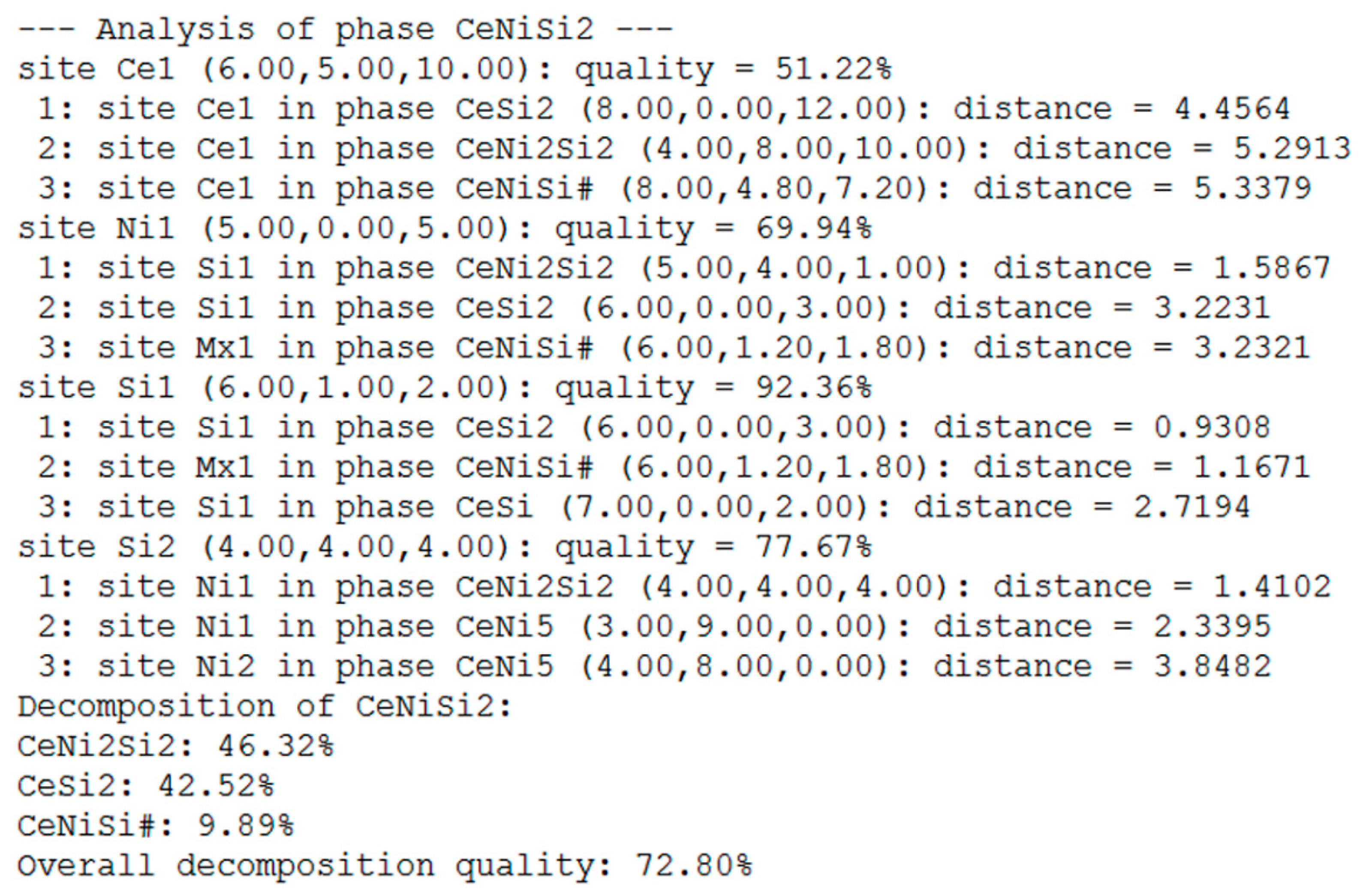
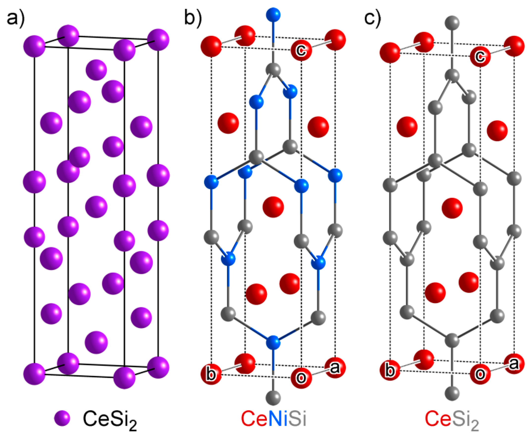
  101. Another difference between CeSi2 and Ce(Ni,Si)2 lies in their cell parameters: CeSi2 has tetragonal symmetry, so its a and b parameters are restricted to be equal (a = b = 4.156 Å), while Ce(Ni,Si)2 does not have such a symmetry constraint (a = 4.039 Å, c = 4.287 Å). For all three phases in the structural series, their two shorter cell axis lengths are almost equal, so the atomic CEs in CeSi2 is less distorted from the target atomic CEs compared to Ce(Ni,Si)2. This explains why CeSi2 takes up a higher weight than Ce(Ni,Si)2 in the decomposition of Ce3Ni2Si8 and CeNiSi2.
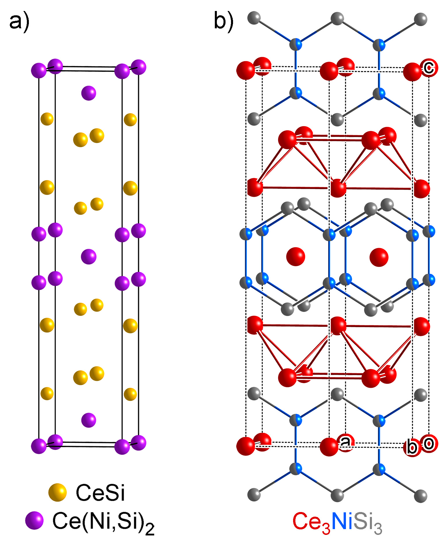
  102. One might notice that these three structures have very similar cell parameters to those of Ce3NiSi3 in Group A1: They all have tall and skinny unit cells with pseudo-tetragonal shapes. However, among these structures, Ce3NiSi3 is the only one that contains the CeSi type Ce double layers, and does not contain any of the CeNi2Si2-type fragments common in the Group A2 phases. Therefore, Ce3NiSi3 should be categorized as a member of Group A1, as is correctly pointed out by PRINCEPS.
Figure 1. Comparison of CE polyhedra with similar descriptor values: (a) The trigonal bipyramid and square pyramid. (b) The tricapped trigonal prism and capped square antiprism. The polyhedra are oriented to highlight the structural similarities between the members of each pair.
Crystals 06 00035 g001
Figure 2. The chemical index values calculated using Pauling electronegativity values and metallic radii (when available) across the periodic table. Covalent radii are used for those non-metal elements that do not have a standard metallic radius.
Crystals 06 00035 g002
Figure 3. Illustration of how the choice of C I 0 affects the R sym values for pairs of elements. The three curves correspond to different C I 0 values. Δ C I values for the pairs Fe-Co, Ni-Ga and Ca-Tl are shown for calibration.
Crystals 06 00035 g003
Figure 4. The solid state compounds with known crystal structures in the Ce-Ni-Si phase diagram at 673 K (above 33.3 at. % Ce) or 1073 K (below 33.3 at. % Ce) [62].
Crystals 06 00035 g004
Figure 5. Similarity dendrogram of all binary phases in the Ce-Ni-Si system generated by PRINCEPS. Each major branch (labeled 1 through 4) corresponds to a cluster of similar binary phases. The x-axis shows the distance between clusters: branches joining at a shorter distance bear higher similarities to each other.
Crystals 06 00035 g005
Figure 6. A snapshot of PRINCEPS output for CeNiSi2 [84], taken from the MATLAB command window.
Crystals 06 00035 g006
Figure 7. The structural relationship between CeNi5 and CeNi4Si: (a) the CeNi5 unit cell; (b) the CeNi4Si unit cell; (c) the subcell–supercell relationship between the two unit cells viewed down the c axis, with depth cueing showing atoms with z = 0.5 (faded atoms) and z = 0 (solid atoms); and (d) the site projection map of CeNi4Si onto CeNi5. In (ac), different colors correspond to different element types while in (d), the color indicates the reference phase the site is projected onto.
Crystals 06 00035 g007
Figure 8. Structural comparison of Ce2Ni3Si5 and CeNi2Si2: (a) the CeNi2Si2 unit cell; (b) the Ce2Ni3Si5 unit cell, oriented so that the Ce CEs are aligned with those of CeNi2Si2 in (a); (c) the subcell–supercell relationship between the two unit cells, viewed down the c axis of CeNi2Si2 and the a axis of Ce2Ni3Si5; and (d) the color-coded site projection map of Ce2Ni3Si5 onto CeNi2Si2. See the caption of Figure 7 for plotting conventions.
Crystals 06 00035 g008
Figure 9. Description of Ce14Ni6Si11 as a structural intergrowth between CeSi and Ce(Ni,Si)2: (a) a color-coded site projection map of Ce14Ni6Si11 onto CeSi (yellow) and Ce(Ni,Si)2 (purple); (b) the Ce14Ni6Si11 unit cell, showing a Ce(Ni,Si)2-type domain and a CeSi-type region adjacent to it, with depth cueing showing atoms with z = 0.5 (solid atoms) and z = 0 (faded atoms); (c) the CeSi unit cell; and (d) the Ce(Ni,Si)2 unit cell.
Crystals 06 00035 g009
Figure 10. Ce6Ni7Si4 as a structural intergrowth of CeSi and CeSi2: (a) the site projection map of Ce6Ni7Si4 onto CeSi (yellow) and CeSi2 (purple); (b) the resulting interpretation of the Ce6Ni7Si4 structure; and the CeSi-type layer and the CeSi2-type layer rotated to the same orientation as (c) the reference phases to better illustrate their similarities.
Crystals 06 00035 g010
Figure 11. The CeNi9Si4 structure: (a) The site projection map of CeNi9Si4 onto Ni3Si (yellow) and CeNi5 (purple). (b) Comparison of the CEs of Ni1 in Ni3Si (cuboctahedral) and Ni3 in CeNi9Si4 (icosahedral). Notice that only a very small distortion is required to change the cuboctahedron into an icosahedron.
Crystals 06 00035 g011
Figure 12. The structural similarity dendrogram generated by PRINCEPS. The x-axis is the distance between clusters: branches joining at a shorter distance bear higher similarities to each other. Using a distance cutoff of 2.0, the ternary phases can be clustered into four groups (A1, A2, A3 and B), plus some remaining Isolated Phases.
Crystals 06 00035 g012
Figure 13. Map of the Ce-Ni-Si ternary phases generated by PRINCEPS. Connections between each ternary phase and any other phase (binary or ternary) with a PRINCEPS distance shorter than 1.2 are shown. Group labels and shaded regions are added manually to highlight the distribution of different groups across the phase diagram. Note: Ce(Ni,Si)2 and CeNi2Si2 both fall within the shaded region of Group A2, but are in fact members of the reference phase library.
Crystals 06 00035 g013
Figure 14. One structural series in the Group A1 structures comprised of Ce6Ni2Si3, Ce5Ni2Si3 and Ce15Ni4Si13: (ac) the site projection map of the three structures onto CeSi (yellow) and Ce(Ni,Si)2 (purple); (df) the unit cells of the three structures, showing the two triangular Ce(Ni,Si)2-type domains within the unit cell and the CeSi-type interfaces in between them; (gi) larger portions of the structures, highlighting the six-fold symmetry and the additional Ni atoms filling the voids where the interfaces meet. Depth cueing is applied to panels (di) to distinguish between atoms with z = 0.5 (solid atoms) and z = 0 (faded atoms).
Crystals 06 00035 g014
Figure 15. The Ce7Ni2Si5 structure as a CeSi-Ce(Ni,Si)2 intergrowth: (a) The site projection map of Ce7Ni2Si5 onto CeSi (yellow) and Ce(Ni,Si)2 (purple). (b) Structural interpretation of the Ce7Ni2Si5 unit cell following these results, with depth cueing showing atoms with z = 0.5 (solid atoms) and z = 0 (faded atoms). Triangular Ce(Ni,Si)2 domains nearly identical to those found in Ce6Ni2Si3 are joined together through CeSi interfaces into slabs. (c) The additional atoms between adjacent slabs form trigonal prisms (yellow polyhedra, only one face visible in the figure) and a smaller fragment of the CeSi structure.
Crystals 06 00035 g015
Figure 16. The Ce3NiSi3 structure as an intergrowth of the structures CeSi and Ce(Ni,Si)2: (a) The site projection map of Ce3NiSi3 onto CeSi (yellow) and Ce(Ni,Si)2 (purple). (b) Structural description of Ce3NiSi3, highlighting the alternation of Ce(Ni,Si)2 slabs and CeSi double layers.
Crystals 06 00035 g016
Figure 17. The CeNiSi structure, an ordered ternary variant of CeSi2: (a) the projection map of CeNiSi onto CeSi2 (purple); (b) the CeNiSi unit cell; and (c) the CeSi2 unit cell.
Crystals 06 00035 g017
Figure 18. A structural series within Group A2: Ce3Ni2Si8, CeNiSi2 and Ce3Ni4Si4. (a) The Ce3Ni2Si8 structure, with projection map on the left and structural interpretation on the right, highlighting its A-B-A-A-B-A stacking of layers, with A = CeNi2Si2 (yellow) and B = Ce(Ni,Si)2 (purple); (b) the CeNiSi2 structure, with A-B-A-B stacking; (c) the Ce3Ni4Si4 structure, with B-A-B-B-A-B stacking; and (d) the two reference phases, CeNi2Si2 and Ce(Ni,Si)2, along with the CeSi2 structure, an alternative way of stacking B layers. Note that A/B/B’ nomenclature becomes sufficient for specifying the structures of these compounds when we introduce the restriction that the layers should be shifted relative to each other along a and b so that Ce positions are shared at the interfaces, and the connectivity of the Ni/Si network is maintained.
Crystals 06 00035 g018
Figure 19. Structural description of Group B: (a) the NaZn13-type structure of CeNi8Si5, with the CsCl-type packing of Ce atoms and Ni/Si icosahedra highlighted; (b) the snub cube coordination polyhedron of the Ce atoms in CeNi8Si5; (c) the CeNi9Si4 structure: note the ordered occupation of Ni and Si atoms; and (d) the CeNi6Si6 structure, where in contrast to the other two structures, the Ni/Si icosahedra are empty.
Crystals 06 00035 g019
Figure 20. Structural description of the isolated phases: (a) the Ce2Ni15Si2 structure, showing alternative honeycomb and Kagome layers, Ce-centered CE polyhedra and the Ni-Ni dumbbells; (b) the Ce2Ni17Si5 structure, highlighting one 22-coordination polyhedron; and (c) the Ce3Ni6Si2 structure, illustrating its segregation into Ce6 octahedral clusters, separated by an interface network of Ni and Si atoms.
Crystals 06 00035 g020
Table 1. CE descriptor values for different coordination polyhedra.
CE Polyhedron TypeCN c 0 (s) c 1 (p) c 2 (d) c 3 (f) c 4 (g)
tetrahedron41.128002.2251.723
square planar41.12801.26202.807
trigonal bipyramid51.41100.1761.8562.567
square pyramid51.4110.040.3281.7892.584
octahedron61.6930003.878
trigonal prism61.69300.5411.5292.176
pentagonal bipyramid71.97400.10303.398
capped trigonal prism71.9740.2740.9720.9162.972
cube82.2570003.447
square antiprism82.25700.51402.113
bisdisphenoid82.25700.0510.1962.913
tricapped trigonal prism92.53900.0191.2390.438
capped square antiprism92.5390.1680.0381.4690.033
bicapped cube102.82100.84402.91
bicapped square antiprism102.82100.51901.276
icosahedron123.3850000
cuboctahedron123.3850001.939
anticuboctahedron123.385000.6810.987
bicapped pentagonal prism123.38500.28200.379
Table 2. List of reference structures for PRINCEPS analysis.
Reference PhaseStructure TypePearson SymbolSpace Group
Ni3SiAuCu3cP4 P m 3 ¯ m
CeSiFeBoP8 P n m a
CeSi2ThSi2tI12 I 4 1 / a m d
CeNi5CaCu5hP6 P 6 / m m m
Ce(Ni,Si)2AlB2hP3 P 6 / m m m
CeNi2Si2ThCr2Si2tI10 I 4 / m m m
Table 3. Distance matrix between the reference phases.
DistanceNi3SiCeSiCeSi2CeNi5Ce(Ni,Si)2CeNi2Si2
Ni3Si02.6932.7372.7112.6962.964
CeSi2.69301.9252.4122.0882.154
CeSi22.7371.92502.2271.0141.906
CeNi52.7112.4122.22702.0191.746
Ce(Ni,Si)22.6962.0881.0142.01901.754
CeNi2Si22.9642.1541.9061.7461.7540
Table 4. Data from the PRINCEPS output for CeNi4Si.
SiteCN VectorQualityReference PhaseReference SiteCN VectorDistance
Ce1(2.00, 14.00, 4.00)99.01%CeNi5Ce1(2.00, 18.00, 0.00)0.9775
CeNi2Si2Ce1(4.00, 8.00, 10.00)3.6373
Ce(Ni,Si)2Ce1(8.00, 4.80, 7.20)5.4135
Ni1(3.00, 7.00, 2.00)94.22%CeNi5Ni1(3.00, 9.00, 0.00)0.8292
CeNi2Si2Ni1(4.00, 4.00, 4.00)2.3017
CeNi5Ni2(4.00, 8.00, 0.00)3.2811
Ni2(4.00, 6.00, 2.00)90.27%CeNi5Ni2(4.00, 8.00, 0.00)1.0008
CeNi5Ni1(3.00, 9.00, 0.00)3.2016
CeNi2Si2Ni1(4.00, 4.00, 4.00)3.7154
Si1(4.00, 8.00, 0.00)81.88%CeNi5Ni2(4.00, 8.00, 0.00)1.2924
CeNi5Ni1(3.00, 9.00, 0.00)3.2767
CeNi2Si2Ni1(4.00, 4.00, 4.00)3.8280
overall decomposition91.64%CeNi5weight:99.89%
CeNi2Si2weight:0.11%
Ce(Ni,Si)2weight:0.00%
Table 5. Data for selected sites from the PRINCEPS output of Ce2Ni3Si5 a.
SiteCN VectorQualityReference PhaseReference SiteCN VectorDistance
Ce1(4.00, 7.00, 10.00)76.39%CeNi2Si2Ce1(4.00, 8.00, 10.00)3.0627
CeNi5Ce1(2.00, 18.00, 0.00)3.6569
CeSi2Ce1(8.00, 0.00, 12.00)5.3249
Ni2(5.00, 0.00, 5.00)72.01%CeNi2Si2Si1(5.00, 4.00, 1.00)1.5344
CeSi2Si1(6.00, 0.00, 3.00)3.1804
Ce(Ni,Si)2Mx1(6.00, 1.20, 1.80)3.1999
Si1(4.00, 4.00, 4.00)69.17%CeNi2Si2Ni1(4.00, 4.00, 4.00)1.6321
CeNi5Ni1(3.00, 9.00, 0.00)2.5067
Ce(Ni,Si)2Mx1(6.00, 1.20, 1.80)3.7712
Si2(4.00, 3.00, 5.00)72.35%CeNi2Si2Ni1(4.00, 4.00, 4.00)1.5506
CeNi5Ni1(3.00, 9.00, 0.00)2.1857
CeNi5Ni2(4.00, 8.00, 0.00)3.8041
overall decomposition63.12%CeNi2Si2weight:80.69%
CeNi5weight:10.79%
Ce(Ni,Si)2weight:4.97%
a Unabridged results for this and other phases discussed in Section 3 can be found in the Supporting Information.
Table 6. Data for selected sites from the PRINCEPS output of Ce14Ni6Si11.
SiteCN VectorQualityReference PhaseReference SiteCN VectorDistance
Ce1(10.00, 2.00, 5.00)87.38%CeSiCe1(10.00, 0.00, 7.00)3.2659
CeSi2Ce1(8.00, 0.00, 12.00)5.2884
CeNi2Si2Si1(5.00, 4.00, 1.00)6.3912
Ce8(8.00, 6.00, 6.00)93.58%Ce(Ni,Si)2Ce1(8.00, 4.80, 7.20)1.8547
CeSi2Ce1(8.00, 0.00, 12.00)3.7543
CeNi2Si2Ce1(4.00, 8.00, 10.00)5.6059
Ni1(6.00, 0.00, 3.00)95.07%CeSi2Si1(6.00, 0.00, 3.00)0.7839
Ce(Ni,Si)2Mx1(6.00, 1.20, 1.80)0.8749
CeSiSi1(7.00, 0.00, 2.00)2.8443
Si1(7.00, 1.00, 1.00)85.46%CeSiSi1(7.00, 0.00, 2.00)1.1839
CeSi2Si1(6.00, 0.00, 3.00)2.6832
Ce(Ni,Si)2Mx1(6.00, 1.20, 1.80)2.7863
overall decomposition81.33%CeSiweight:65.34%
Ce(Ni,Si)2weight:18.70%
CeSi2weight:15.93%
Table 7. Data for selected sites from the PRINCEPS output of Ce6Ni7Si4.
SiteCN VectorQualityReference PhaseReference SiteCN VectorDistance
Ce3(8.00, 5.00, 4.00)72.74%CeSiCe1(10.00, 0.00, 7.00)3.2659
CeSi2Ce1(8.00, 0.00, 12.00)5.2884
Ce(Ni,Si)2Ce1(8.00, 4.80, 7.20)5.5187
Ce4(8.00, 8.00, 4.00)85.61%CeSi2Ce1(8.00, 0.00, 12.00)2.4999
Ce(Ni,Si)2Ce1(8.00, 4.80, 7.20)3.7168
CeSiCe1(10.00, 0.00, 7.00)5.6100
Ni1(6.00, 2.00, 1.00)65.24%CeSi2Si1(6.00, 0.00, 3.00)1.7046
Ce(Ni,Si)2Mx1(6.00, 1.20, 1.80)1.8492
CeSiSi1(7.00, 0.00, 2.00)2.5276
Ni4(7.00, 0.00, 2.00)55.83%CeSiSi1(7.00, 0.00, 2.00)1.9447
CeSi2Si1(6.00, 0.00, 3.00)2.7660
Ce(Ni,Si)2Mx1(6.00, 1.20, 1.80)2.8333
overall projection51.91%CeSi2weight:39.05%
CeSiweight:37.59%
Ce(Ni,Si)2weight:13.32%
Table 8. Data for selected sites from the PRINCEPS output of CeNi9Si4.
SiteCN VectorQualityReference PhaseReference SiteCN VectorDistance
Ce1(0.00, 16.00, 8.00)31.31%CeNi5Ce1(2.00, 18.00, 0.00)5.8858
CeNi2Si2Ce1(4.00, 8.00, 10.00)6.6348
Ce(Ni,Si)2Ce1(8.00, 4.80, 7.20)8.1575
Ni1(2.00, 6.00, 4.00)12.07%CeNi5Ni1(3.00, 9.00, 0.00)4.0759
Ni3SiNi1(0.00, 8.00, 4.00)4.0763
Ni3SiSi1(0.00, 12.00, 0.00)4.0996
Ni3(0.00, 8.00, 4.00)92.19%Ni3SiNi1(0.00, 8.00, 4.00)0.9236
Ni3SiSi1(0.00, 12.00, 0.00)1.2999
CeNi5Ni2(4.00, 8.00, 0.00)4.4683
overall projection19.79%Ni3Siweight:44.77%
CeNi5weight:41.66%
CeNi2Si2weight:9.01%
Table 9. Categorization of Ce-Ni-Si ternary phases.
Group AGroup A1Ce14Ni6Si11 (mC124, C 2 / m ), Ce6Ni2Si3 (hP22, P 6 3 / m ), Ce5Ni2Si3 (hP40, P 6 3 / m ), Ce15Ni4Si13 (hP64, P 6 3 / m ), Ce7Ni2Si5 (oP56, P n m a ), Ce3NiSi3 (oI14, I m m m )
Group A2CeNiSi (tI12, I 4 1 m d ), Ce2Ni3Si5 (oI40, I b a m ), Ce3Ni2Si8 (oS26, C m m m ), CeNiSi2 (oS16, C m c m ), Ce3Ni4Si4 (oI22, I m m m )
Group A3Ce6Ni7Si4 (oP68, P b c m )
Group BCeNi9Si4 (tI56, I 4 / m c m ), CeNi8Si5 (cF112, F m 3 ¯ c ), CeNi6Si6 (tI52, P 4 / n b m )
Isolated PhasesCeNi4Si (oS12, C m m m ), Ce2Ni15Si2 (hR57, R 3 ¯ m ), Ce2Ni17Si5 (tI48, I 4 1 / a m d ), Ce3Ni6Si2 (cI44, I m 3 ¯ m )
Table 10. PRINCEPS decomposition weights for the Group A1 phases.
PhaseQualityComponent 1Weight 1Component 2Weight 2Component 3Weight 3
Ce14Ni6Si1181.33%CeSi65.34%Ce(Ni,Si)218.70%CeSi215.93%
Ce6Ni2Si364.63%CeSi91.01%Ce(Ni,Si)25.00%CeSi23.79%
Ce5Ni2Si374.45%CeSi79.43%Ce(Ni,Si)213.93%CeSi26.53%
Ce15Ni4Si1380.09%CeSi68.43%Ce(Ni,Si)224.59%CeSi26.90%
Ce7Ni2Si573.17%CeSi89.82%CeSi26.66%Ce(Ni,Si)23.48%
Ce3NiSi390.80%CeSi57.89%Ce(Ni,Si)231.82%CeSi210.28%
Table 11. PRINCEPS decomposition weights for the Group A2 phases.
PhaseQualityComponent 1Weight 1Component 2Weight 2Component 3Weight 3
Ce2Ni3Si563.12%CeNi2Si280.69%CeNi510.79%Ce(Ni,Si)24.97%
CeNiSi94.12%CeSi285.54%Ce(Ni,Si)214.44%CeSi0.01%
Ce3Ni2Si876.58%CeNi2Si267.46%CeSi224.66%Ce(Ni,Si)26.54%
CeNiSi272.80%CeNi2Si246.32%CeSi242.52%Ce(Ni,Si)29.89%
Ce3Ni4Si482.01%CeSi242.73%CeNi2Si231.58%Ce(Ni,Si)224.87%
Table 12. PRINCEPS decomposition weights for the Group B phases.
PhaseQualityComponent 1Weight 1Component 2Weight 2Component 3Weight 3
CeNi9Si419.79%Ni3Si44.77%CeNi541.66%CeNi2Si29.01%
CeNi8Si520.36%CeNi548.97%Ni3Si37.85%CeNi2Si29.96%
CeNi6Si618.70%CeNi564.12%CeNi2Si221.61%Ce(Ni,Si)27.01%
Table 13. Distance matrix between Group B phases.
DistanceCeNi8Si5CeNi9Si4CeNi6Si6
CeNi8Si500.4771.147
CeNi9Si40.47701.139
CeNi6Si61.1471.1390
Table 14. PRINCEPS analysis result on the isolated phases.
PhaseQualityComponent 1Weight 1Component 2Weight 2Component 3Weight 3
CeNi4Si91.64%CeNi599.89%CeNi2Si20.11%Ce(Ni,Si)20.00%
Ce2Ni15Si225.30%CeNi584.20%Ni3Si11.07%CeNi2Si24.17%
Ce2Ni17Si519.88%CeNi563.59%Ni3Si24.48%CeNi2Si29.43%
Ce3Ni6Si248.37%CeNi560.12%CeSi14.97%CeNi2Si211.02%

