Article

Microstructure Characterization in Individual Texture Components by X-Ray Line Profile Analysis: Principles of the X-TEX Method and Practical Application to Tensile-Deformed Textured Ti

1
Department of Materials Physics, Eötvös Loránd University Budapest, Pázmány P. sétány 1/A, H-1117 Budapest, Hungary
2
Materials Performance Centre, Department of Materials, The University of Manchester, Manchester M13 9PL, UK
3
Section of Materials and Surface Engineering, Department of Mechanical Engineering, Technical University of Denmark, Produktionstorvet 425, 2800 Kgs. Lyngby, Denmark
*
Author to whom correspondence should be addressed.
Crystals 2020, 10(8), 691; https://doi.org/10.3390/cryst10080691
Submission received: 30 June 2020 / Revised: 1 August 2020 / Accepted: 6 August 2020 / Published: 10 August 2020
(This article belongs to the Special Issue X-ray and neutron Line Profile Analysis of Microstructures)

Abstract

:
A novel X-ray diffraction-based method and computer program X-TEX has been developed to determine the microstructure in individual texture components of polycrystalline, textured materials. Two different approaches are presented. In the first one, based on the texture of the specimen, the X-TEX software provides optimized specimen orientations for X-ray diffraction experiments in which diffraction peaks consist of intensity contributions stemming from grain populations of separate texture components in the specimen. Texture-specific diffraction patterns can be created by putting such peaks together from different measurements into an artificial pattern for each texture component. In the second one, the X-TEX software can determine the intensity contributions of different texture components to diffraction peaks measured in a particular sample orientation. According to this, peaks belonging mainly to one of the present texture components are identified and grouped into the same quasi-phase during the evaluation procedure. The X-TEX method was applied and tested on tensile-deformed, textured, commercially pure titanium samples. The patterns were evaluated by the convolutional multiple whole profile (CMWP) procedure of line profile analysis for dislocation densities, dipole character, slip systems and subgrain size for three different texture components of the Ti specimens. Significant differences were found in the microstructure evolution in the two major and the random texture components. The dislocation densities were discussed by the Taylor model of work hardening.

Graphical Abstract

1. Introduction

Crystallographic texture plays a significant role in the mechanical response of structural materials [1,2]. In structural materials with hexagonal close-packed (hcp) structure, especially in Ti, Zr, Mg and their alloys, the role of texture is even more significant [3,4,5,6,7,8]. Texture influences most of the mechanical, physical and chemical properties of polycrystalline materials, rendering these properties anisotropic [1]. From the practical point of view, the anisotropy in these properties may or may not be a desirable feature [2]. Improvement in the mechanical properties such as strength, ductility or toughness can often be achieved through microstructural control or texture optimization. Depending on the manufacturing procedure, the microstructure of the different texture components can be very different. Therefore, the quantitative analysis of the microstructural parameters prevailing in individual texture components is indispensable for a better understanding of the mechanical, physical and chemical properties of structural materials.
X-ray and neutron diffraction line profile analysis has proven to be a powerful tool for characterizing the microstructure of crystalline materials [9,10,11,12,13]. Software packages have been developed to determine the microstructural parameters from the shape of the diffracted peaks using Marquardt–Levenberg (ML) optimization [12,13]. In the convolutional multiple whole profile (CMWP) procedure the measured diffraction patterns are matched by simulated diffraction patterns consisting of several convoluted defect-specific profile functions. The defect-related theoretical profile functions are tuned by the physically mandatory minimum number of parameters. These parameters are the median, m, and the variance, σ LN , of a log-normal size distribution function in the size profile, the dislocation density, ρ, the dislocation arrangement parameter, M and, in case of hcp materials, the fractions of prevailing slip systems in the strain profile and the fault density, α SF or β Tw for stacking faults or twin boundaries in the planar defect profile [13,14]. In more complex cases like hexagonal materials or multiple phases the ML procedure alone may cause uncertainties. The CMWP method has been improved recently using a new approach in which the ML and a Monte-Carlo statistical method are combined in an alternating manner [15]. The new CMWP procedure eliminates uncertainties and provides globally optimized parameters of the microstructure.
CMWP can be used for describing the microstructure of individual texture components separately, only if each diffraction peak originates from a single texture component only. There are two ways to achieve this: (1) create a texture-specific diffraction pattern (TSDP) for each texture component by cutting diffraction peaks corresponding to the same texture component from one or more measured patterns and putting them together, (2) grouping the peaks in a measured pattern and handling them as multiple quasi-phases where each quasi-phase corresponds to a separate texture component.
In our previous works we developed procedures to separate X-ray diffraction peaks belonging to both random and one major texture components. The microstructural parameters were determined in the random and major texture components in a strongly textured AZ31-type Mg alloy deformed at different temperatures by evaluating diffraction patterns of more than one quasi-phase [16] and in tensile-deformed Zr by evaluating TSDPs [17]. However, in the procedures described in [16,17] only one major texture component was considered and the identification of diffraction peaks corresponding to the same texture component is valid only in a close range around the 0° azimuth angle of the scattered beam. Therefore, if the measured data are collected by a two-dimensional detector, only a limited fraction of the Debye–Scherrer (DS) rings can be used in these evaluation schemes.
The characterization of the microstructure in four major texture components separately by neutron diffraction line profile analysis has been developed by Ungár et al. [11]. Although that method provides the separation of diffraction peaks for multiple texture components in the case of neutron diffraction experiments, X-ray diffraction geometry is more complex from the point of view of the peak identification procedure. The neutron diffraction geometry in the SMARTS engineering diffractometer [18], and in a number of other similar diffractometers at spallation neutron sources [19,20,21] has two detectors positioned at angles +90° and −90° relative to the incoming neutron beam and the diffraction patterns are collected by the method of time of flight (TOF) in each detector. Since the diffraction angles are the same for all diffraction peaks, it is relatively simple to calculate the intensity contribution recorded by the detectors for the different texture components as detailed in [11]. In the case of X-ray diffraction with a parallel beam geometry both in laboratory and synchrotron measurements, when the beam is monochromatic, the scattered intensity distribution depends on both the diffraction angle and the azimuth angle. In order to get a diffraction pattern, the intensity distribution is often integrated alongside the azimuth angle, especially in synchrotron measurements. If one wants to determine the contributions of different texture components for a diffraction peak in a measured pattern in general, one needs to calculate the intensity as a function of the diffraction and azimuth angles integrated over a certain azimuthal interval of the DS rings.
In this work we present the principles and the practice of a general method to determine the microstructural parameters in multiple texture components separately in the case of parallel-beam geometry X-ray diffraction setups. Based on the principles of the method a computer software package, X-TEX, has been developed. The present work aims to determine differences between the microstructures in different, coexisting texture components, in this manner, X-TEX differs from texture analysing software as MTEX [22] or ATEX [23]. The method will be tested and illustrated by determining the dislocation densities, dipole character, prevailing slip systems and subgrain sizes in tensile-deformed, textured, commercially pure Ti.

2. Principles of the X-TEX Method

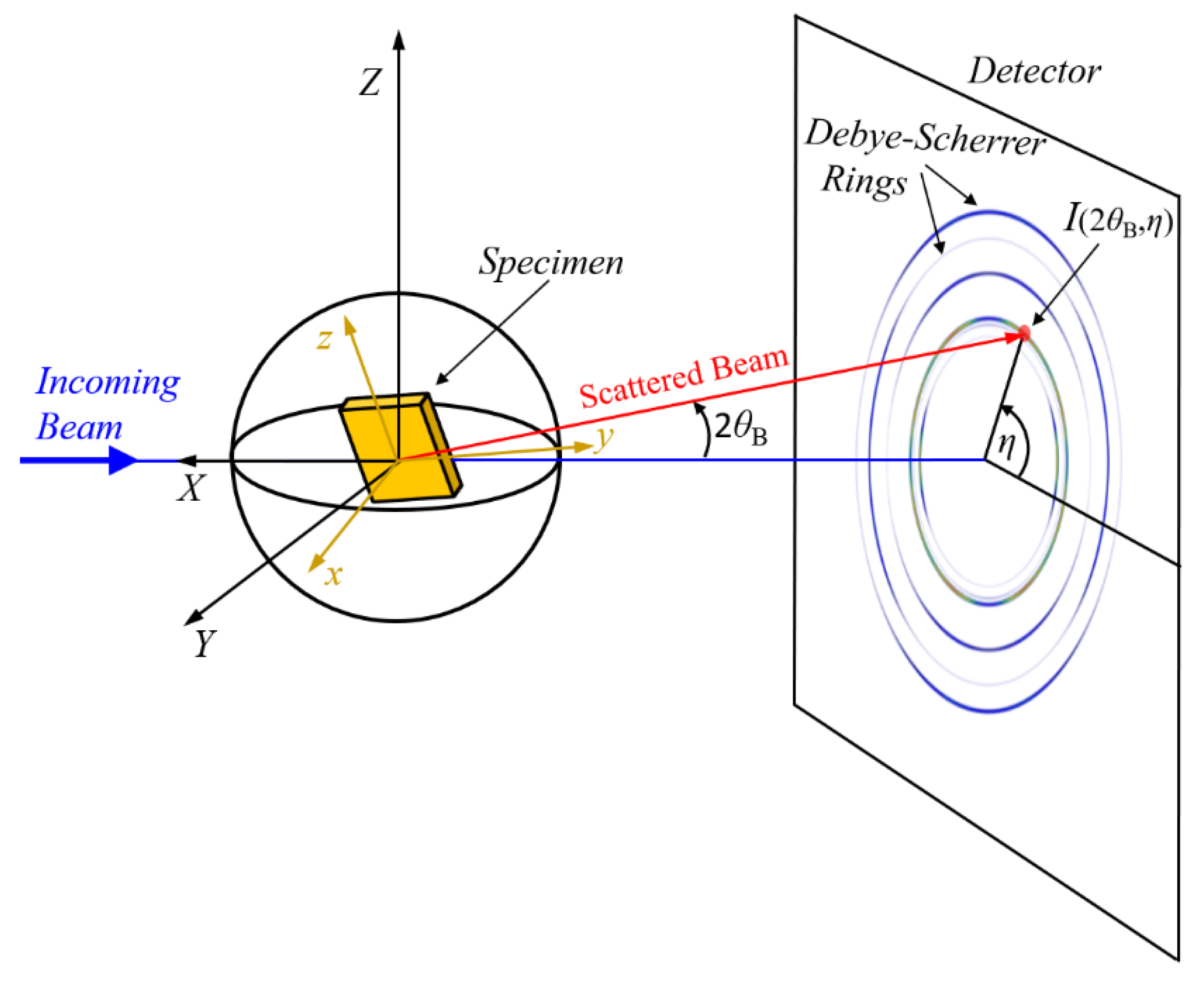
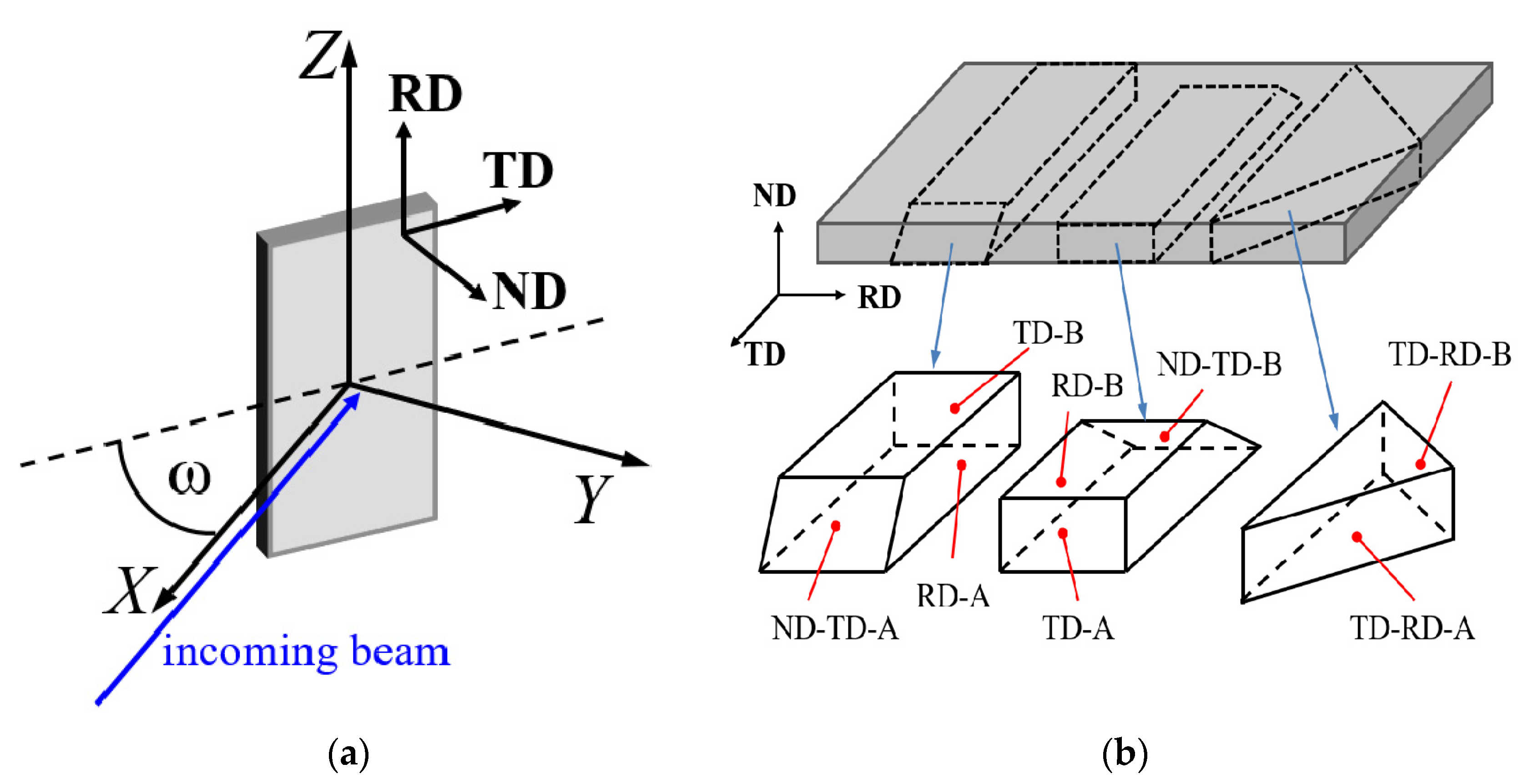
In the X-TEX procedure we simulate the texture using Gaussian distributions around the ideal orientations of specific texture components. With this method we calculate the scattered X-ray intensity contribution from each texture component at any point along the DS rings. The laboratory and the specimen Cartesian coordinate systems, K L = { X , Y   Z } and K s = { x , y , z } , are shown in Figure 1. The laboratory coordinate system is defined so that the positive X-axis is parallel to the incoming X-ray beam showing toward the X-ray source, and the positive Z-axis is pointing upwards. Initially K L and K s coincide, i.e., xX, yY and zZ. In an orthogonal coordinate system, the unit vectors, e h k l , normal to the crystallographic hkl planes in cubic or hcp crystals are:
e h k l = 1 h 2 + k 2 + l 2 ( h , k , l )   or   e h k l = d h k l ( 2 h + k 3 a ,   k a , l c )
where d h k l is the spacing of hkl planes and a and c are the lattice parameters in the hcp crystal. In the case of hcp crystals, the unit cell is positioned in the following manner: the a 1 basis vector has an angle of 30° with the x -axis and a 2 and c are parallel to the y - and z -axis, respectively.
The ideal orientation of a texture component, R ^ ( φ 1 ,   Φ ,   φ 2 )   ϵ   S O ( 3 ) is interpreted as a three-dimensional rotation matrix with z-x-z convention:
R ^ ( φ 1 ,   Φ ,   φ 2 ) = R ^ z ( φ 1 ) R ^ x ( Φ ) R ^ z ( φ 2 )
where the Eulerian angles φ 1 , Φ and φ 2 describe the rotation between the crystallographic and the sample coordinate system K s . The specimen orientation in K L is described by another rotation matrix with Z-X-Z convention:
R ^ ( α , β , γ ) = R ^ Z ( α ) R ^ X ( β ) R ^ Z ( γ )
where α , β and γ are the Eulerian angles of the specimen rotation in K L . Rotating the specimen by α , β and γ angles, the normal vectors of the hkl planes for an ideal orientation of the ith texture component will be
e h k l i = R ^ ( α , β , γ )   R ^ ( φ 1 i , Φ i , φ 2 i ) e h k l .
Denote the unit vector in the direction of the diffraction vector in K L as s h k l :
s h k l = 1 2 sin ( θ B ) ( 1 cos ( 2 θ B ) ,   sin ( 2 θ B ) cos ( η ) , sin ( 2 θ B ) sin ( η ) )
where θ B is the diffraction angle of hkl planes according to Bragg’s law and η is the azimuth angle of the scattered beam as it can be seen in Figure 1. The hkl plane of a crystal will scatter the X-ray beam into ( 2 θ B , η ) direction only if the normal vector of the plane is pointing in the s h k l direction. This means that in the ( 2 θ B , η ) direction the diffracted X-ray intensity is proportional to the volume fraction of grains oriented in this manner. Their relative volume fraction is obtained by assuming a Gaussian distribution of orientations around the ideal orientation of the ith texture component:
Ψ i = A i · exp ( ( s x e x i ) 2 2 Δ 2 ) · exp ( ( s y e y i ) 2 2 Δ 2 ) · exp ( ( s z e z i ) 2 2 Δ 2 ) = A i G x G y G z
where Δ 2 is the variance of the distribution and A i is a normalization factor taking into account the f i [ 0 , 1 ] volume fraction of grains belonging to the ith texture component:
A i = f i / π π 0 π G x G y G z sin ϑ   d ϑ d φ
where ϑ and φ are polar coordinates. The total intensity of the hkl reflection in the ( 2 θ B , η ) direction including the contribution of the random texture component is:
I ( 2 θ B , η ) tot = K ( i { h k l } | F h k l | 2 Ψ i + f r 4 π { h k l } | F h k l | 2 ) = i I ( 2 θ B , η ) i + I ( 2 θ B , η ) r
where f r is the volume fraction of the random texture component, K is a coefficient that includes the Lorentz-polarization and the absorption correction, F h k l is the structure factor and the { h k l } summation goes over permutations of the hkl indices. Experimental diffraction patterns for line profile analysis are obtained by integrating the intensity distribution measured with a two-dimensional detector along the η azimuth angle. Therefore, one has to integrate the theoretical intensity distribution I ( 2 θ B , η ) tot of Equation (8) over an [ η min , η max ] interval as well:
I ( 2 θ B ) tot = η min η max I ( 2 θ B , η ) tot d η = i I ( 2 θ B ) i + I ( 2 θ B ) r .
the theoretical diffraction pattern produced by any modelled texture for any specimen orientation is given by Equation (9) and consists of several peaks.
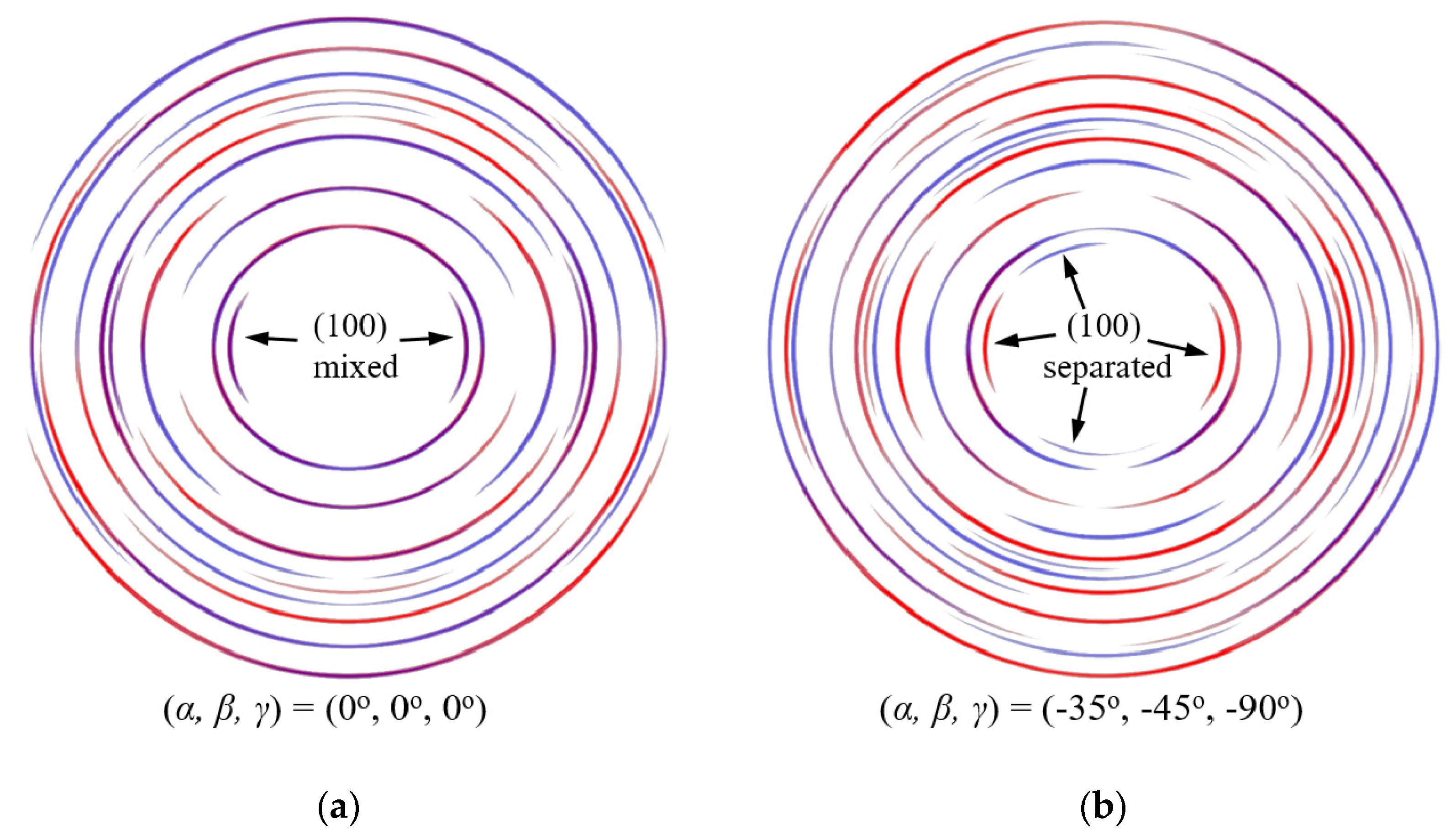
When a polycrystalline material is texture free, the intensity along DS rings is constant. Texture causes variations of the intensity along the rings and the diffracted intensity originates from different texture components as illustrated in Figure 2. Figure 2a shows the diffracted intensity resulting from two texture components ( φ 1 ,   Φ ,   φ 2 ) = ( 90 ° , ± 40 ° , 0 ° ) for which the intensities of the (100) reflection overlap. Figure 2b, however, shows the diffracted intensity distribution resulting from the same two texture components for a different specimen orientation, where the intensities along the DS ring of the (100) reflection are well separated into sections consisting of contributions from the individual single texture components. Integration over the entire ring or partial η integration over an erroneously chosen [ η min , η max ] range causes mixed diffraction peaks consisting of contributions from different texture components. The goal is to find those specimen orientations which provide for as many as possible separated intensity distributions along the hkl rings from which diffraction peaks corresponding to one single texture component only can be obtained. Since texture is usually not infinitely sharp, it is to be expected that peaks mainly corresponding to one texture component will also have some contribution from other texture components. The overlap of scattered intensity from different texture components can be considered by taking into account the angular spread and the volume fraction of grains of different texture components. The intensity contributions for hkl peaks provided by grains belonging to the ith texture component are described with the χ h k l i = I ( 2 θ B ) i / I ( 2 θ B ) tot intensity ratios. Peaks are considered to correspond to the investigated texture component, if their intensity ratio is larger than a chosen threshold value χ 0 .
There are two possibilities to evaluate the peaks belonging to the same texture component with the CMWP software. The first possibility is to put individually selected peaks (obtained from integrating the intensity distributions along an hkl ring over a specific η interval) together creating a texture-specific diffraction pattern (TSDP). These peaks can be selected either from different measurements or from the same measurement by integrating the intensities over different η intervals for each peak. The second possibility is to integrate the DS rings over the same η range for each hkl ring and group the peaks into different quasi-phases in the CMWP procedure. The advantages of this (quasi) multiple-phase evaluation against the TSDP method are: (1) there is no need to cut out peaks, thus overlapping peaks can also be evaluated; and (2) the TSDP may require in general more than one measurement, where the second method does not. The disadvantage is that peaks have lower χ values, thus, the contributions of alien texture components will be higher. In this work both methods will be applied to tensile-deformed, textured titanium.

3. Specifications of the X-TEX Software

Based on the principles outlined above, a software package, X-TEX has been developed. The programs are written in C++ and C# languages for Windows operation system. The software package and the source codes are freely available on the http://metal.elte.hu/~berci/X-TEX.html website.
First, the following data must be specified as input based on texture measurements: (1) the Eulerian angles ( φ 1 ,   Φ ,   φ 2 ) of the ideal orientation for each texture component; (2) the full width at half maximum (FWHM = 2 2 ln 2 Δ ) of the Gaussian distributions in Equation (6); and (3) the volume fraction of grains belonging to each texture component. In addition, there is an opportunity to link several texture sub-components (where each sub-component is of a Gaussian distribution around a slightly different ideal orientation) belonging to the same major texture component in order to be able to describe more complex textures, such as fibre texture. X-TEX can handle cubic, hexagonal and trigonal crystal systems.
Given the input data, there are multiple possible functions of X-TEX:
(a)
It is possible to plot a pole figure for any hkl. This gives the option to check whether the input data are correct and produces the same type of pole figures as, for instance, measured ones.
(b)
A detector image (DS rings) can be plotted in order to be able to compare calculated and measured X-ray diffraction data visually. For this, the experimental parameters and settings as well as the hkl indices of the peaks to be plotted need to be specified. The intensity in each point of the detector is calculated using Equation (8). In this plot anisotropic peak broadening is not considered, the peak shapes are approximated with a Gaussian function and all the peaks have the same width.
(c)
X-TEX can calculate the χ h k l i intensity ratios for each texture component for the measured peaks after integration over a specified [ η min , η max ] range, given the sample orientation and measurement settings.
(d)
There is a scanning function in X-TEX. Using this function, the sample orientations can be optimized in order to allow measuring X-ray diffraction peaks corresponding to a chosen texture component with minimal contribution of other components. The software calculates a specimen rotation map, where the scattered X-ray intensity of a specific hkl ring integrated over a [ η min , η max ] range is calculated for different sample orientations and plotted as a function of rotation angles. This plot allows the optimal specimen orientation where the intensity of the hkl diffraction peak is the largest with minimal contribution of other alien texture components to be selected. As a result, a series of measurements can be planned in order to measure as many peaks as possible belonging to different texture components separately.
(e)
The parameters used to describe textures in this method can be determined by common texture measurements, but X-TEX also has an option of using a Monte-Carlo algorithm to fit these parameters based on X-ray diffraction measurements according to how the intensity varies along the DS rings.

4. Experimental

4.1. Samples

In order to test the X-TEX method, four plates of commercially pure titanium of ASTM grade 1 were received as-rolled and annealed. Three of them were tensile deformed at room temperature with the strain rate of 2.2 × 10⁻⁴ 1/s as detailed in [24]. True plastic strain of 2%, 10% and 23% were achieved for these specimens. The tensile deformation was parallel to the original rolling direction (RD) and the normal direction (ND) is perpendicular to the largest flat surface of the plates.

4.2. Texture Measurements

Orientation maps for texture analysis were collected by electron backscatter diffraction (EBSD) using a Tescan Mira3 FEG-SEM (Tescan, Brno, Czech Republic) fitted with an Oxford Instruments Symmetry EBSD detector at a voltage of 15 keV. The size of each map was about 500 × 500 μm2 and the step size utilized was 0.2 μm. The pole figures shown in Figure 3 (in general agreement with the ones presented in [24]) were generated using the MTEX toolbox in MATLAB [25]. The figures show a typical TD split texture for cold-rolled Ti with two symmetrical major texture components. This type of deformation texture in the case of Ti is a result of the combination of prismatic { 100 } 110 and basal { 001 } 110 slips [26]. The maximal pole densities of the (001) basal poles are tilted about ±(35–40)° from ND towards TD for all specimens. The basal poles keep their positions, but the distribution slightly broadens with increasing strain. The slight variation between the intensity of both symmetric poles is considered insignificant and not analysed further. However, remarkable changes are resolved by the two other, (110) and (100) pole figures. The dominating (110) direction along RD is replaced by a dominating (100) direction indicating a rotation of the crystallographic lattice by 30° around the c-axis during tensile deformation. The texture is different in all specimens which has to be taken into account during the separation procedure of the diffraction peaks.

4.3. X-Ray Diffraction Experiments

X-ray diffraction measurements were carried out in a special high-resolution diffractometer dedicated to line profile analysis operated at a copper rotating anode X-ray generator (RA-MultiMax9, Rigaku, Tokyo, Japan). A symmetrical Ge(110) single crystal was used as primary beam monochromator eliminating CuKα2 radiation and a CuKα1 X-ray beam with a wavelength of λ = 0.15406 nm was used [27]. The scattered radiation was detected by two-dimensional curved imaging plate (IP) detectors with linear spatial resolution of 50 μm. The distances between the stationary specimens and the IPs were 100 mm or 300 mm. The shorter IP distance was used only to obtain texture parameters with the X-TEX method, and the larger IP distance was used for line profile analysis providing higher angular resolution and negligible instrumental effect. The footprint of the beam on the specimen was about 0.2 × 2.0 mm2 and the beam divergence was 5 × 10⁻⁴ rad. The instrumental correction in this setup above 200 mm IP distance is negligible since the instrumental peak broadening causes only about 1012 m−2 uncertainty in the dislocation density values [28].
Two measurement series were devised for line profile analysis in order to match the different evaluation types as illustrated in Figure 4. In the first series, two measurements were performed on the ND surface of all four specimens as shown in Figure 4a. In this case, the patterns were evaluated using the multiple phase option of CMWP according to the χ values calculated by X-TEX for each peak. In this manner, it was possible to follow the microstructure evolution during deformation in all texture components separately. In the second series, measurements were designed and performed for the 23% deformed specimen in such a way that the diffraction peaks have higher χ values. For this purpose, three pieces were cut out from the plate as shown in Figure 4b. Altogether eight measurements were carried out on different surfaces indicated in Figure 4b. Peaks belonging to the same texture components were selected from these eight measurements so that it was possible to create a TSDP for each texture component. In our analysis, the specimen coordinate system was defined as x‖TD, y‖RD and z‖ND and the specimen orientation in the laboratory coordinate system before any rotation was defined as X‖TD, Y‖RD and Z‖ND. The Eulerian angles of the specimen rotations in case of the different measurements are listed in Table 1. The specimen surfaces for X-ray diffraction measurements were mechanically polished and finally chemically etched with hydrogen fluoride in order to remove any damaged surface layer.

5. Evaluation of the X-Ray Diffraction Experiments

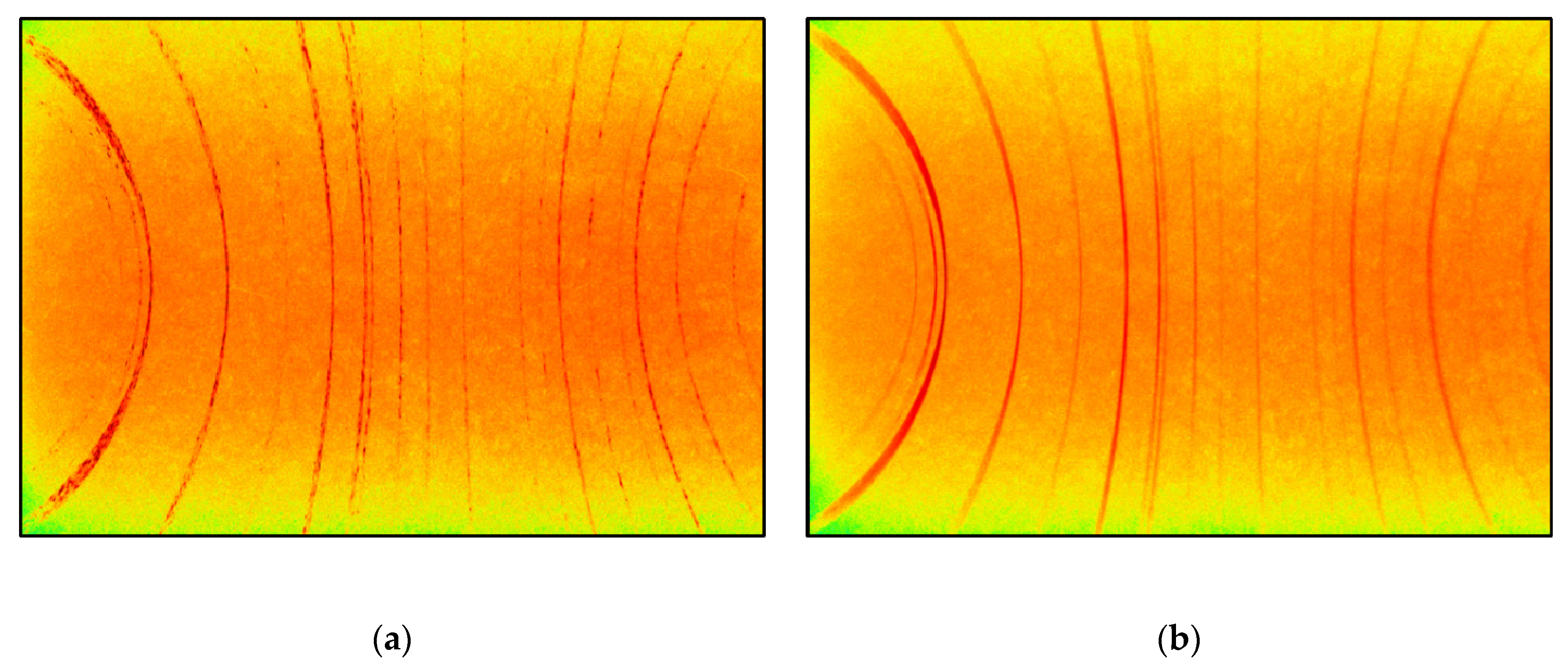
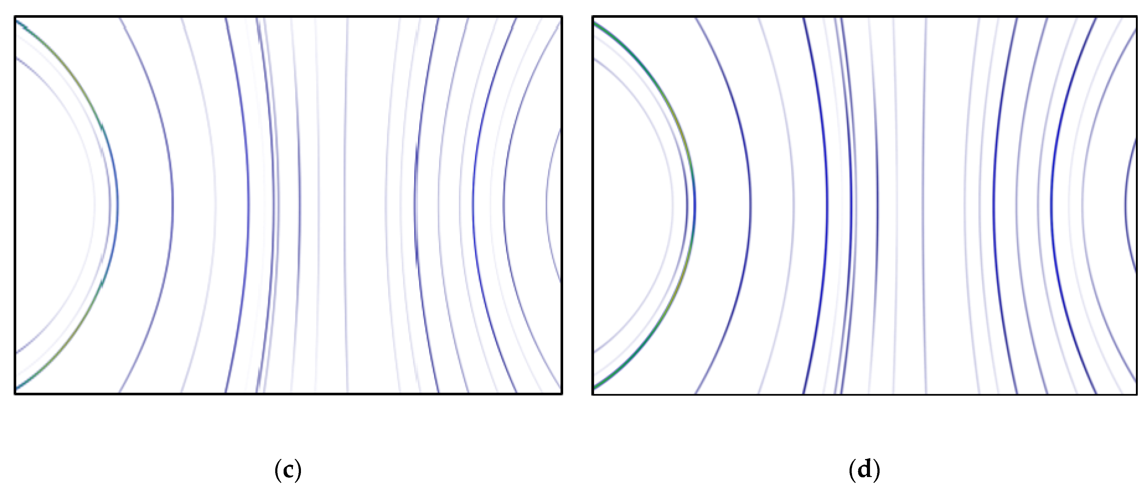
Prior to the line profile measurements with long sample-detector distance of 300 mm, the scattered X-ray intensity distribution was recorded using a shorter (100 mm) sample-detector distance for all specimens with ND-A sample orientation in order to measure larger parts of the DS rings. From these measurements, the parameters used to describe the texture in the X-TEX method were determined according to the intensity variation along the DS rings. IP readouts for the as-received and the 23% tensile-deformed specimen are shown in Figure 5a,b, respectively. The two images are very similar because of the similar texture, however, small differences can be recognized in the case of some arcs. It will be shown later, that these differences have great importance in the separation procedure of the peaks. It is noted that in the case of the as-received image, intensity maxima are visible because of the large undistorted grains in this specimen. The strong line broadening toward the edge of the IPs in the vertical direction is an instrumental effect from the horizontal width of the beam, which occurs because of the relatively small specimen-IP distance. This problem automatically disappears at larger distances between specimen and IP. The texture parameters are determined from these measurements by dividing the images into several horizontal stripes. The measured intensity of the hkl diffraction peak in the Nth stripe, I N ,   h k l meas is obtained by integrating the intensity distribution along the DS arc in the range of the stripe. The X-TEX software varies the texture parameters with a Monte-Carlo algorithm and calculates the intensity of diffraction peaks in each stripe with different texture parameters. The obtained results, I N ,   h k l calc are compared with the measured intensities for all of the stripes and DS rings. The texture parameters are optimized by minimizing the sum of squared residuals (SSR):
S S R = N , h k l ( I N ,   h k l meas I N ,   h k l calc ) 2 .
Calculated detector images based on the optimized texture parameters for the as-received and the 23% tensile-deformed specimen are shown in Figure 5c,d, respectively.
The texture parameters, i.e., the Eulerian angles φ 1 , Φ and φ 2 of the ideal orientation of each of the major texture components, the f r volume fraction of the random texture component and the full width at half maximum (FWHM = 2 2 ln 2 Δ ) of the Gaussian distribution defined in Equation (6), determined by X-TEX are listed in Table 2.
The f i volume fractions of the major texture components are considered equal for the symmetrical components with respect to RD according to the measured pole figures. Based on the measured pole figures, each of the two major texture components (one with positive Φ , the other with negative Φ ) was produced from two subcomponents for more precise description of the texture. Calculated pole figures based on the texture parameters listed in Table 2 are plotted in 
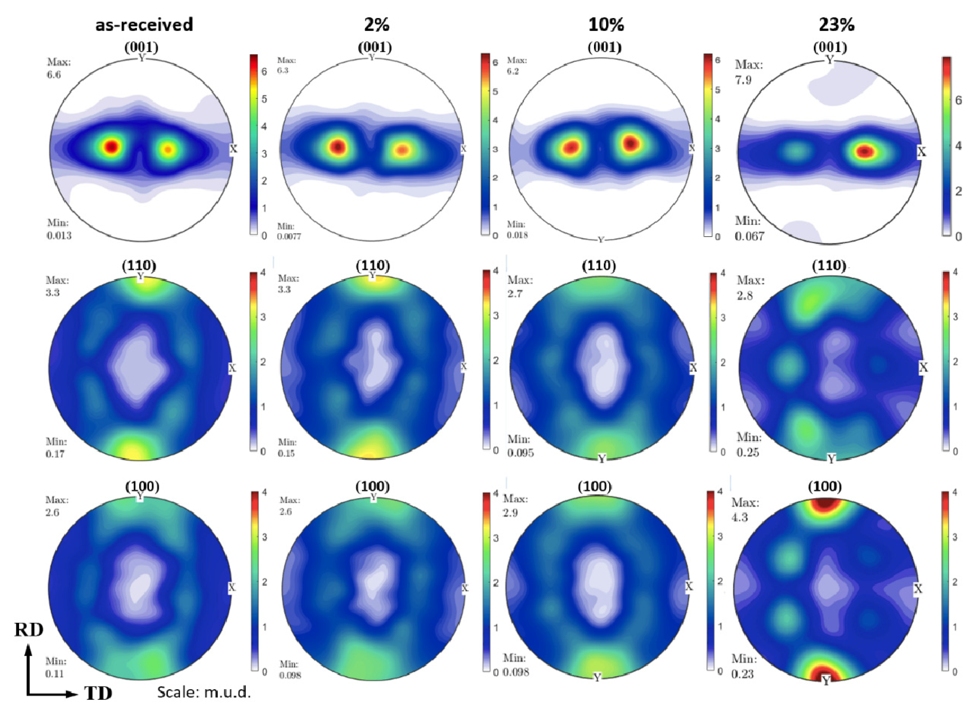
Figure 6. It can be seen that the calculated pole figures based on texture parameters determined from X-ray diffraction measurements are in good agreement with pole figures measured by EBSD (if the slightly different frequency of the symmetrical components with respect to RD is ignored) and show, for instance, the replacement of the (110) direction by a (100) direction along RD.
Knowing the parameters of the texture, X-ray diffraction measurements were performed for line profile analysis with a larger (300 mm) sample-detector distance to achieve higher angular resolution and negligible instrumental effect. Line profiles were obtained by integrating the intensity distributions along the corresponding DS rings. The diffraction patterns were evaluated by the CMWP procedure [15]. The measured diffraction pattern, I ( 2 θ ) meas is matched by theoretically calculated and convoluted profile functions representing the effects of size, I h k l S , distortion, I h k l D and planar defects, I h k l P as well as instrumental effects, I h k l inst :
I ( 2 θ ) meas = h k l I h k l S I h k l D I h k l P I h k l inst + I BG
where the asterisk stands for convolution and I BG is the background intensity. The instrumental contribution was deemed unnecessary, as the present instrumental conditions do not require the use of any corrections. The nature of line broadening caused by crystallite size, distortion and planar faults are essentially different, so fitting multiple whole measured profiles considering these physical effects simultaneously makes a powerful tool to characterize the microstructure. The size profile, I h k l S is determined by assuming a log-normal size distribution with median m and logarithmic variance σ LN [10]. The area-weighted average crystallite size, x area , was calculated from the median and variance of the distribution as x area = m   exp ( 2.5 σ LN 2 ) [29]. x area represents the coherently scattering domain size which is closer to the subgrain or dislocation cell size than to crystallographic grain size. The strain profile, I h k l D is given by its Fourier transform [30]:
FT ( I h k l D ) = exp { 2 π 2 L 2 g 2 ε g , L 2 }
where g is the absolute value of the diffraction vector and L is the Fourier variable. The mean square strain caused by restrictedly random dislocation distributions in crystals is given by the Wilkens function f ( L / R e )   [31]:
ε g , L 2 ρ C h k l b 2 4 π f ( L / R e )
where ρ, b, C h k l and Re are the dislocation density, the absolute value of the Burgers vector, the hkl dependent contrast factor and the effective outer cut-off radius of dislocations, respectively. Since the absolute value of Re depends on the dislocation density ρ, a dimension-free parameter, M = R e ρ was introduced to describe the dislocation arrangement. The smaller the value of M , the stronger is the correlation between dislocations of opposite sign. In this manner, smaller M indicates a stronger dipole character. If dislocations of all possible Burgers vectors in a particular slip mode are equally populated, the dislocation contrast factors can be averaged over the permutations of the corresponding hkl indices. In the hexagonal system this is given as [32]:
C ¯ h k l i = C ¯ h k 0 i ( 1 + q 1 i x + q 2 i x 2 )
where x = ( 2 / 3 ) ( l / g a ) 2 , q 1 i   and q 2 i are parameters depending on the ith slip plane family, the elastic properties of the material and the c/a ratio, C ¯ h k 0 i is the average contrast factor of the ith slip plane family corresponding to the hk0 type reflections, and a is the lattice constant in the basal plane. The CMWP procedure provides measured parameter values q 1 meas and q 2 meas . Matching of the measured q 1 , 2 meas and theoretically calculated q 1 , 2 i values can provide the relative fractions h a , h c + a   and h c of the a , c + a and c type of dislocations as detailed in [33]. The I h k l P planar defect profiles are parameterized as a function of fault probabilities for the different stacking faults and twin boundaries [14]. In [14], the effect of twinning on the diffraction patterns in hexagonal materials is worked out for the {101}<102> and {112}<113> compressive, and {102}<101> and {111}<116> tensile twin systems. Since the CMWP evaluation gave zero twin probability in all the specimens for all twinning modes, these values are not presented in this paper (note that this is not in conflict with the frequency of twin boundaries up to 30% reported in [24] based on EBSD measurements. The latter twin boundary frequency refers to the fraction of twin boundaries of all high angle boundaries, whereas profile analysis determines the probability of twin boundaries occurring on all possible twinning planes). At room temperature, several twinning modes have been observed in commercially pure titanium, e.g., [24,34]. However, the effect of twinning cannot be seen in the X-ray line profiles unless the average distance between twin boundaries is smaller than about 2 μm corresponding to a twin probability of at most 0.01%.
In order to follow the microstructure evolution during deformation in the different texture components separately, two measurements were carried out on the ND surface for all specimens denoted as ND-A and ND-B. The A and B notation distinguishes pairs of measurements which are symmetrical from the point of view of texture and the separation procedure of the diffraction peaks. This means that the χ values of the two major texture components become swapped between the two measurements of the pair, while the χ values of the random texture component are the same. Using this method, particular hkl peaks correspond to component #1 when measured on surface A, but to component #2 when measured on surface B, respectively. In this manner, several hkl peaks are measured for both major texture components and the peaks for the random component are measured twice so better statistics for the microstructural parameters can be achieved during the CMWP evaluation. The ND-A and ND-B diffraction patterns were evaluated simultaneously in the fitting procedure with the same parameter values for the individual texture components. The χ values of the two major and the random texture components for the hkl peaks in the case of the as-received and the 23% tensile-deformed specimens in the ND-A measurement are listed in Table 3. The χ values in the case of the ND-B measurements are exactly the same except the swap between the two major components. The patterns were evaluated using the multiple phase option of CMWP, where the individual peaks were assigned to the three different quasi-phases according to their χ values calculated by X-TEX. In Table 3 it can be seen that peaks mainly correspond to one texture component, but also have some contribution from other texture components. Peaks are considered to belong to one of the major texture components if χ 1 , 2 > 60 % and to the random component if χ r > 40 % . These values are highlighted with bold numbers in the table. The limit of 40% intensity contribution for the random texture component may appear to be a low value, however for this limit the scattered intensity stems from grains tilted at least 30° from the ideal orientation of the major texture components. Table 3 shows that the intensity contributions for some hkl peaks are remarkably different between the as-received and the 23% tensile-deformed specimen; two peaks (201 and 203) are actually assigned to different texture components.
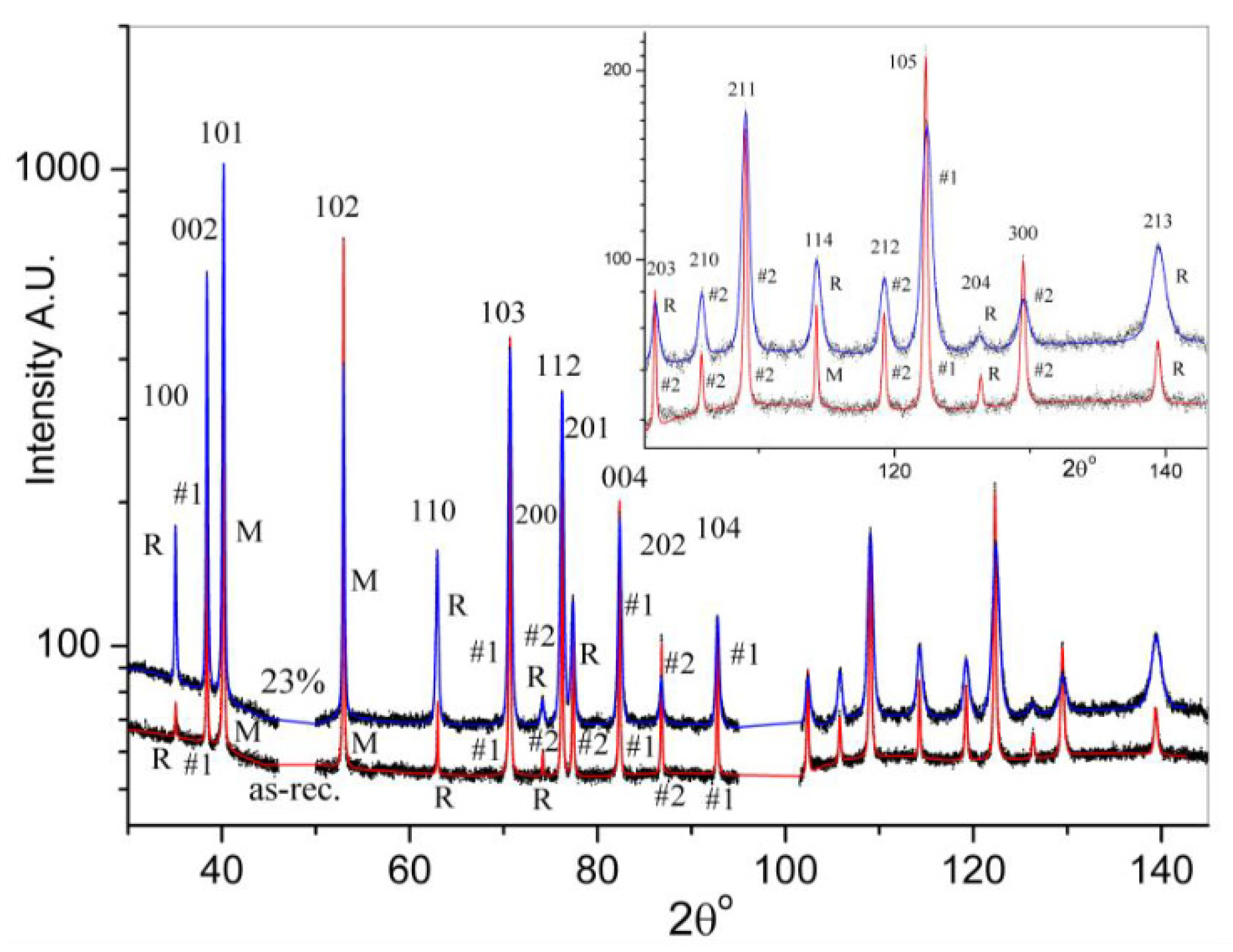
The diffraction patterns of the as-received and 23% tensile-deformed specimens corresponding to the ND-A measurement are shown in Figure 7. The peaks in the patterns were grouped into multiple phases in the CMWP method according to their χ values so that each quasi-phase corresponds to a single texture component. In order to reveal the shape of the peaks in the whole intensity range better, a logarithmic intensity scale is used. The peaks, which could not be unambiguously assigned to a phase, were fitted as a separate “mixed” phase as well, the results of which are not interpreted. This evaluation with multiple phases is an appropriate method to include overlapping peaks, such as 112 and 201 in Figure 7 as well, even when they are attributed to different phases.
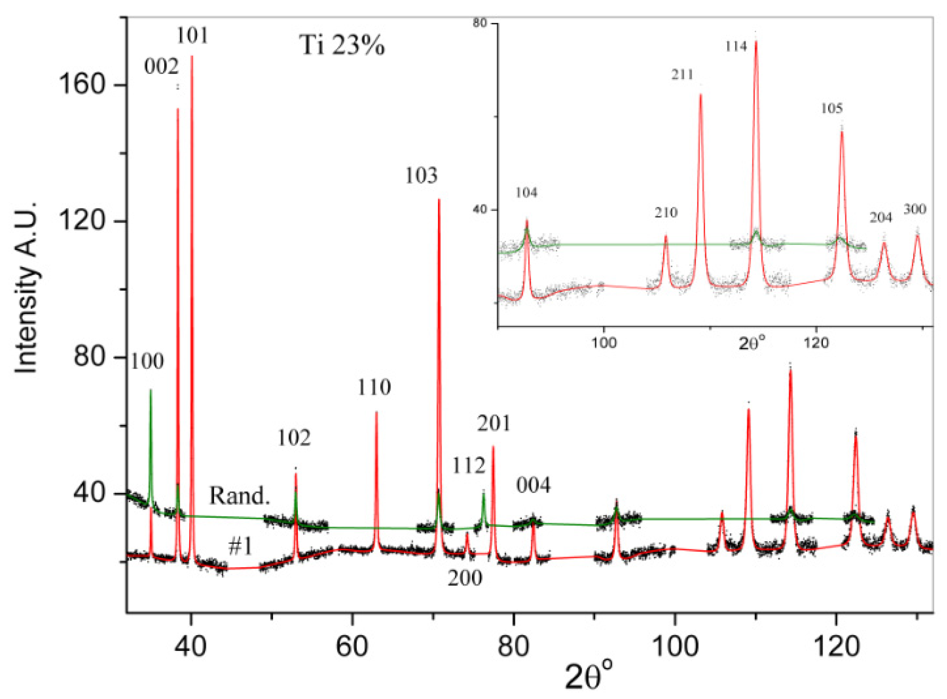
Higher χ values for individual peaks can be obtained by carrying out multiple measurements with different sample orientations. In this manner, texture-specific diffraction patterns (TSDPs) can be created by cutting and putting together peaks with high χ values for each texture component. In the case of the ND-A and ND-B measurements for the 23% tensile-deformed specimen, the average χ value of peaks belonging to the major texture components is 80%, but only 57% for peaks of the random texture component. In order to show the power of using TSDPs, eight measurements were performed for the 23% tensile-deformed specimen in different sample orientations denoted as illustrated in Figure 4b. The χ values of the two major and the random texture components for the hkl peaks in the case of the TSDP measured on different surfaces are listed in Table 4. Using TSDPs, the average χ value was 85% for both the major and the random texture components. In Figure 8, TSDPs for the major texture component #1 and the random texture component are plotted.

6. Results

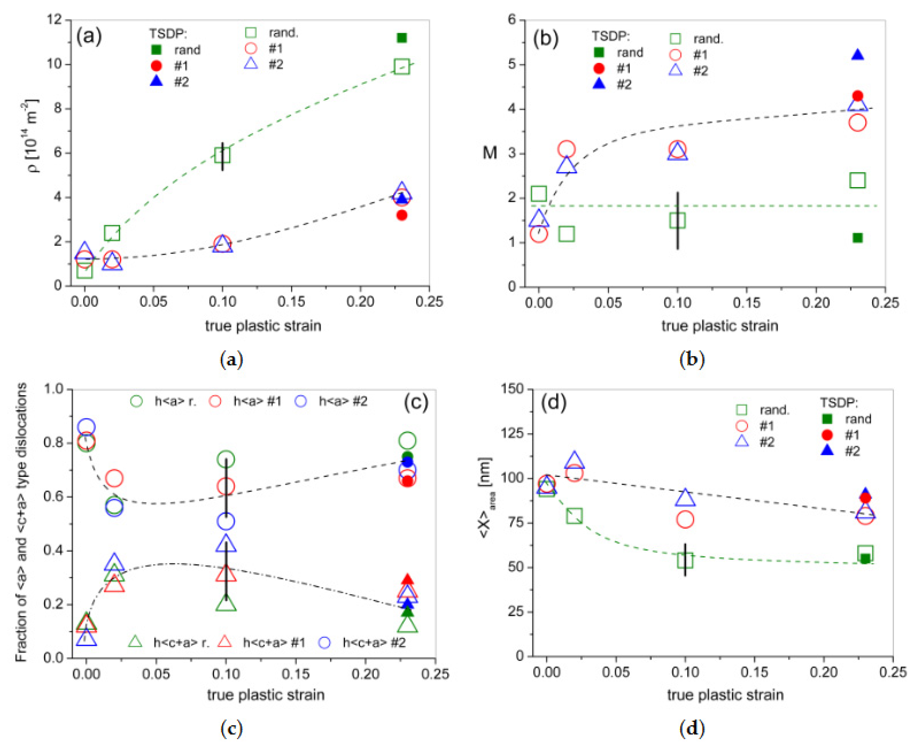
The results of the CMWP evaluation are shown in Figure 9. By combining the Marquardt–Levenberg optimization procedure with a statistical Monte Carlo method, robust optimized parameters are obtained [15]. The resulting values for the microstructural parameters versus the true plastic strain are plotted for the different texture components separately. In addition, the results of the evaluation of the TSDPs for the 23% tensile-deformed specimen are shown in the figures as well. A significant difference was found between the dislocation densities in the random and major texture components (Figure 9a). In the as-received state the dislocation density is the same for all texture components within experimental error. With increasing deformation, the dislocation density increases in all texture components, however, in the random component the increase is significantly, about 2–3 times higher than in the two major components. The difference between the dislocation densities in the random and the two major texture components is slightly higher in case of the TSDP evaluation that consists of peaks with higher χ ratios, however, there is no significant difference between the two methods.
For all texture components, the arrangement parameter M is above 1 indicating rather low screening between the dislocations (Figure 9b). The value of M remains between 1 and 2 during the whole deformation in the random texture component while M increases in the major texture components to about 4 indicating an even weaker screening. Again, the M values obtained from the TSDP evaluation differ slightly more. In the as-received state, there are mainly a type dislocations in the specimen, their fraction is over 80%. As a result of deformation, initially (during the first 2% tensile deformation) the fraction of c + a type dislocations increases and reaches even 40%, then with increasing plastic deformation the a type dislocations become more dominant again. There is no significant difference in this respect between the major and the random texture components (Figure 9c). The area-weighted crystallite size remains almost constant during the first 2% of tensile deformation and decreases after 2% deformation in all components (Figure 9d). The refinement is stronger in the random component, i.e., the crystallite size is under 60 nm in the random component while it is around 90 nm in the major texture components after 23% strain. The microstructural parameters of the two major texture components are equivalent within experimental error during the whole deformation.

7. Discussion

In order to deform a polycrystal homogeneously without producing cracks, at least five independent slip systems need to be activated. For hcp metals this requirement cannot be fulfilled by only a type dislocations since they can provide only four independent slip systems [35,36], therefore twinning or deformation by c + a type dislocations are needed as well [37]. From the CMWP evaluation a vanishing probability for twin boundaries (less than 0.01%) is concluded. This is, however, not in conflict with the observations [24] that about 30% of all high angle boundaries (with mean chord length of 5 µm and above) were identified as twin boundaries. Further evidence from EBSD revealed the occurrence of 64.6° <100> compressive twinning after 2% tensile deformation and additional 84.8° <110> tensile twinning after 10% tensile deformation. Only during the first 2% tensile deformation, no twinning is observed at all. This may explain the observation of a strong increase in c + a type dislocations during the initial deformation stage to achieve compatible deformation during this stage. During later stages, twinning can accommodate part of the deformation and the increase in the density of c + a type dislocations is not as strong any longer. Nevertheless, dislocation accumulation of a type dislocations occurs continuously along with twinning.
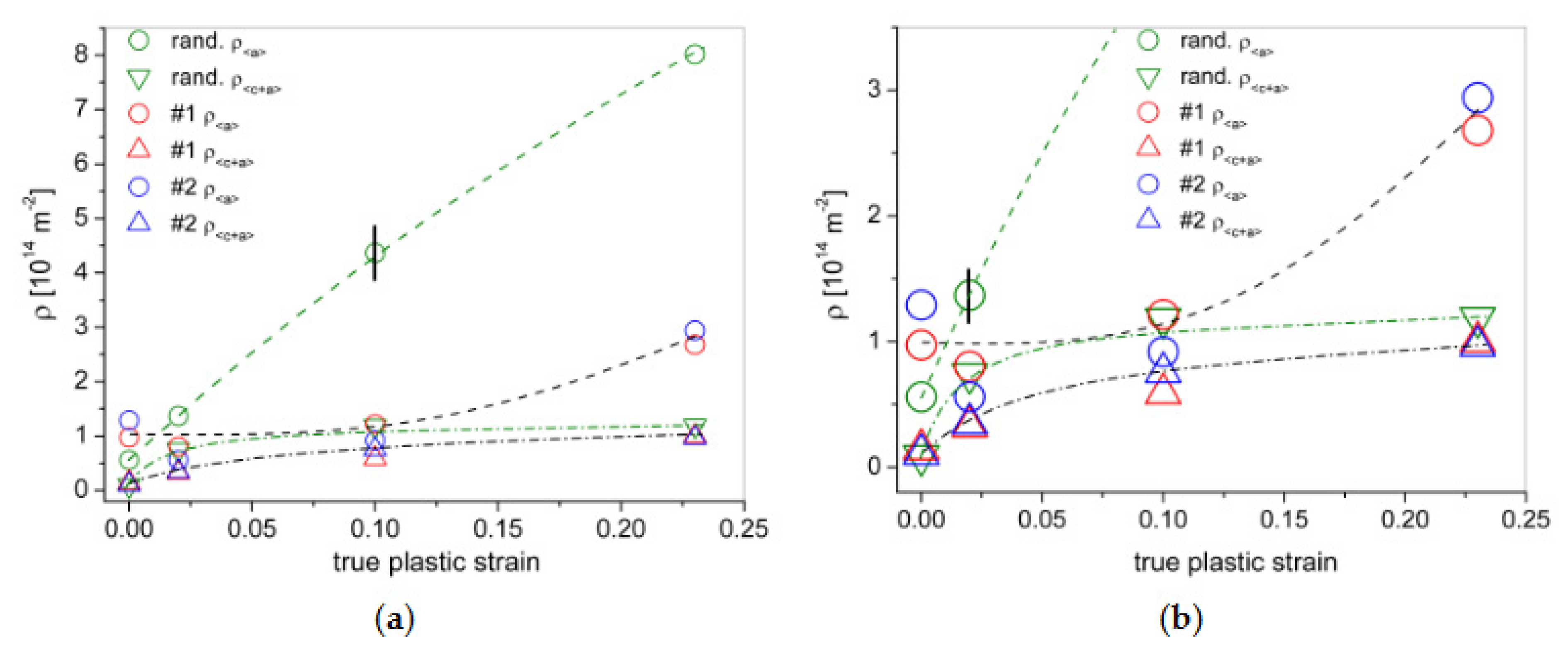
A significant difference between the dislocation densities of the random and the major texture components can be revealed by plotting the densities of a and c + a type dislocations separately. Figure 10a,b shows that while in the random component the amount of a type dislocations gradually increases with deformation, in the major texture components a type slip systems are not activated even at 10% strain, the density of a type dislocations increases only at higher, 23% strain. The reason for this may be the following: It is well known that in CP Ti the main slip systems are prismatic and basal a systems [38], providing altogether four independent slip systems. Although pyramidal a slip can be present as a secondary slip system, the critical resolved shear stress (CRSS) value for this is higher than for pyramidal c + a system [39]. In our case, the Schmid factor of basal a slip is zero for the ideal orientation of both major texture components in the as-received state as well as after 23% tensile deformation and has very small values for orientations close to these orientations. Consequently, the number of independent a type slip systems is higher in the random texture component than in both major texture components causing the development of larger dislocation densities of a type Burgers vectors in the random texture component. The almost constant density of a dislocations in the major texture components at the beginning of the tensile deformation, on the other hand, roots analogously in the vanishing Schmid factor for basal slip for these orientations. With proceeding tensile deformation, an increased activation of prismatic a slip may cause the observed increase in density of a dislocations in the major texture components. Despite the CRSS of c + a dislocations being much higher than that of a dislocations, c + a slip systems must be activated as an increase in the c + a dislocation density is observed during tensile deformation. The initial increase in their density is attributed to the requirement of compatible deformation: without activation of twinning modes, i.e., in the early stage of tensile deformation, compatibility can only be achieved by a certain contribution of c + a slip. With proceeding deformation, the increase in density of c + a dislocations becomes smaller, most likely due to a lower activation of c + a slip systems enabled by simultaneously occurring twinning.
From the arrangement parameters M generally larger than 1, it is concluded that the deformation-induced dislocations do not create dislocation configurations with short screening length as narrow dislocation dipoles in either one of the texture components. There could be several reasons for that: (i) the dislocation density may not be large enough to force the dislocations into low energy configuration with small screening length like dipoles, (ii) the dislocations may not have enough three-dimensional mobility to acquire these configurations, or (iii) the dislocation annihilation might be insufficient to allow their ordering. In the major texture components the dislocation densities are lower than in the random texture component, they show even weaker screening and a larger arrangement parameter.
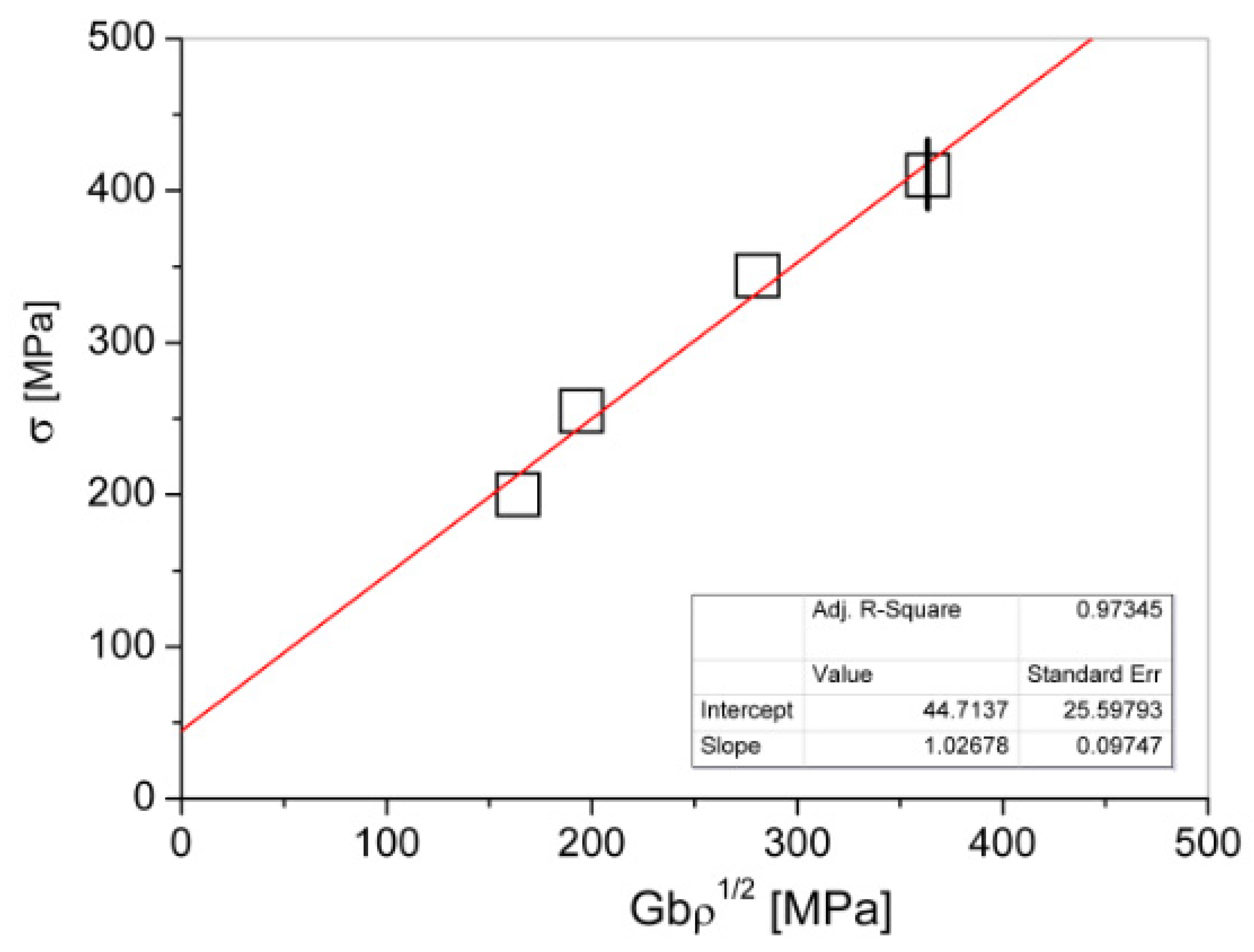
In order to connect microstructure with strength, the flow stress, σ , is correlated with the dislocation densities, ρ , in Figure 11. The dependence can be rationalized using Taylor’s relation [40]:
σ = σ 0 + α M T G b ρ
where σ 0 is a friction stress required to move dislocations, α is an interaction coefficient describing the interactions between dislocations, M T is the Taylor factor for dislocation slip, G = 44 GPa is the shear modulus and b is the length of the Burgers vector averaged according to the fractions of the different types of dislocations.
For the dislocation densities and Burgers vectors volume-averaged values are considered corresponding to the volume fractions of the major and random texture components. The flow stress values are taken from the stress-strain curve in [24]. Using Equation (15), σ 0 , i.e., the intercept with the stress axis and the product α M T , i.e., the slope of the fitted straight line can be obtained as shown in Figure 11. The result of σ 0   = 45 (±26) MPa from this linear fitting is close to the standard value of 78 MPa for well-annealed CP Ti [41]. The M T Taylor factor varies between 2.5 and 5.0 for Ti in literature [42,43]. By knowing the texture, it would be possible in principle to calculate M T on the assumption of c + a and a slip, however it is beyond the scope of the present work. Using the 2.5 and 5.0 extremal values of the Taylor factor we get 0.21 and 0.41 as lower and upper bounds for the coefficient α in good correspondence with expected values from 0.1 to 0.5 in [44]. The good description achieved by Taylor’s relation indicates that dislocations are mainly responsible for the observed work-hardening in spite of the concurrent twinning. This is in accordance with the successful description of the different work-hardening stages by stage wise Voce laws in [24].

8. Conclusions

(1)
In the present work a novel method based on X-ray diffraction has been described which has been developed to characterize the microstructure in individual texture components of textured materials separately. Based on the principles of this method a freely available computer program called X-TEX was devised for planning diffraction experiments in order to measure diffraction peaks mainly corresponding to one texture component.
(2)
The method was applied for tensile-deformed CP Ti specimens with typical cold-rolling texture. Two approaches of X-ray diffraction experiments and evaluation types were presented in which the investigated texture components contribute with lower or higher intensities to diffraction peaks. It was found that both approaches gave very similar results indicating that the method is not particularly sensitive to whether peaks have the maximal possible intensity contribution from a chosen texture component or not.
(3)
Using the new method, it was possible to determine the microstructure evolution during deformation. A significant difference was found between the dislocation densities of the random and the major texture components and a type dislocations contribute dominantly to the dislocation population. It was proven experimentally that the microstructural parameters in the two major texture components are equivalent.
(4)
The dislocation densities were related to the flow stress values using Taylor’s relation. It was found that the dislocation density present was able to rationalize the tensile flow stresses.

Author Contributions

Conceptualization: B.J.; methodology: B.J. and É.Ó.; software: B.J.; formal analysis: B.J. and É.Ó.; investigation: B.J., É.Ó. and M.M.; resources: W.P.; data curation: B.J.; writing—original draft preparation: B.J. and É.Ó.; writing—review and editing: T.U.; review and interpretation: W.P.; supervision: T.U. All authors have read and agreed to the published version of the manuscript.

Funding

This research received no external funding.

Acknowledgments

The research reported in this paper was supported by the Higher Education Excellence Program of the Ministry of Human Capacities of Hungary within the frame of the ELTE University Excellence program (1783-3/2018/FEKUTSTRAT). T. Ungár acknowledges support from EPSRC programme grant MIDAS (EP/S01702X/1). The authors would like to thank Framatome for providing the funding for their student Mia Maric.

Conflicts of Interest

The authors declare no conflict of interest.

References

  1. Kocks, U.F.; Tomé, C.N.; Wenk, H.-R. Texture and Anisotropy: Preferred Orientation in Polycrystals and Their Effect on Materials Properties; Cambridge University Press: Cambridge, UK, 1998. [Google Scholar]
  2. Suwas, S.; Ray, R.K. Crystallographic Texture of Materials (Engineering Materials and Processes); Springer: London, UK, 2014. [Google Scholar]
  3. Ivasishin, O.M.; Semiatin, S.L.; Markovsky, P.E.; Shevchenko, S.V.; Ulshin, S.V. Grain growth and texture evolution in Ti–6Al–4V during beta annealing under continuous heating conditions. Mater. Sci. Eng. A 2002, 337, 88–96. [Google Scholar] [CrossRef]
  4. Karadge, M.; Preuss, M.; Lovell, C.; Withers, P.J.; Bray, S. Texture development in Ti–6Al–4V linear friction welds. Mater. Sci. Eng. A 2007, 459, 182–191. [Google Scholar] [CrossRef]
  5. Garner, A.; Frankel, P.; Partezana, J.; Preuss, M. The effect of substrate texture and oxidation temperature on oxide texture development in zirconium alloys. J. Nucl. Mater. 2017, 484, 347–356. [Google Scholar] [CrossRef]
  6. Moya Riffo, A.; Vicente Alvarez, M.A.; Santisteban, J.R.; Vizcaino, P.; Limandri, S.; Daymond, M.R.; Kerr, D.; Okasinski, J.; Almer, J.; Vogel, S.C. Crystallographic texture and microstructural changes in fusion welds of recrystallized Zry-4 rolled plates. J. Nucl. Mater. 2017, 488, 83–99. [Google Scholar] [CrossRef] [Green Version]
  7. Agnew, S.R.; Yoo, M.H. Using Deformation-Induced Texture as an Alloy/Process Optimization Tool. In Magnesium Technology 2000; Kaplan, H.I., Hryn, J., Clow, B., Eds.; The Minerals, Metals & Materials Society: Warrendale, PA, USA, 2000; pp. 331–339. [Google Scholar]
  8. Suh, B.-C.; Kim, J.H.; Hwang, J.H.; Shim, M.-S.; Kim, N.J. Twinning-mediated formability in Mg alloys. Sci. Rep. 2016, 6, 22364. [Google Scholar] [CrossRef] [Green Version]
  9. Ungár, T.; Dragomir, I.; Révész, Á.; Borbély, A. The contrast factors of dislocations in cubic crystals: The dislocation model of strain anisotropy in practice. J. Appl. Crystallogr. 1999, 32, 992–1002. [Google Scholar] [CrossRef] [Green Version]
  10. Ungár, T.; Gubicza, J.; Ribárik, G.; Borbély, A. Crystallite size distribution and dislocation structure determined by diffraction profile analysis: Principles and practical application to cubic and hexagonal crystals. J. Appl. Crystallogr. 2001, 34, 298–310. [Google Scholar] [CrossRef] [Green Version]
  11. Ungár, T.; Holden, T.M.; Jóni, B.; Clausen, B.; Balogh, L.; Csiszár, G.; Brown, D.W. Dislocation structure in different texture components determined by neutron diffraction line profile analysis in a highly textured Zircaloy-2 rolled plate. J. Appl. Crystallogr. 2015, 48, 409–417. [Google Scholar] [CrossRef]
  12. Scardi, P.; Leoni, M. Whole powder pattern modelling. Acta Crystallogr. A 2002, 58, 190–200. [Google Scholar] [CrossRef]
  13. Ribárik, G.; Ungár, T. Characterization of the microstructure in random and textured polycrystals and single crystals by diffraction line profile analysis. Mater. Sci. Eng. A 2010, 528, 112–121. [Google Scholar] [CrossRef]
  14. Balogh, L.; Tichy, G.; Ungár, T. Twinning on pyramidal planes in hexagonal close packed crystal determined along with other defects by X-ray line profile analysis. J. Appl. Crystallogr. 2009, 42, 580–591. [Google Scholar] [CrossRef]
  15. Ribárik, G.; Jóni, B.; Ungár, T. Global optimum of microstructure parameters in the CMWP line-profile-analysis method by combining Marquardt-Levenberg and Monte-Carlo procedures. J. Mater. Sci. Technol. 2019, 35, 1508–1514. [Google Scholar] [CrossRef] [Green Version]
  16. Jóni, B.; Al-Samman, T.; Chowdhury, S.G.; Csiszár, G.; Ungár, T. Dislocation densities and prevailing slip-system types determined by X-ray line profile analysis in a textured AZ31 magnesium alloy deformed at different temperatures. J. Appl. Crystallogr. 2013, 46, 55–62. [Google Scholar] [CrossRef]
  17. Fan, Z.; Jóni, B.; Xie, L.; Ribárik, G.; Ungár, T. Dislocation structure in textured zirconium tensile-deformed along rolling and transverse directions determined by X-ray diffraction line profile analysis. J. Nucl. Mater. 2018, 502, 301–310. [Google Scholar] [CrossRef]
  18. Bourke, M.A.M.; Dunand, D.C.; Ustundag, E. SMARTS—A spectrometer for strain measurement in engineering materials. Appl. Phys. A Mater. Sci. Process. 2002, 74, s1707–s1709. [Google Scholar] [CrossRef]
  19. Santisteban, J.R.; Daymond, M.R.; James, J.A.; Edwards, L. ENGIN-X: A third-generation neutron strain scanner. J. Appl. Crystallogr. 2006, 39, 812–825. [Google Scholar] [CrossRef]
  20. Wang, X.-L.; Holden, T.M.; Rennich, G.Q.; Stoica, A.D.; Liaw, P.K.; Choo, H.; Hubbard, C.R. VULCAN—The engineering diffractometer at the SNS. Phys. B Condens. Matter 2006, 385, 673–675. [Google Scholar] [CrossRef]
  21. Harjo, S.; Ito, T.; Aizawa, K.; Arima, H.; Abe, J.; Moriai, A.; Iwahashi, T.; Kamiyama, T. Current Status of Engineering Materials Diffractometer at J-PARC. Mater. Sci. Forum 2011, 681, 443–448. [Google Scholar] [CrossRef]
  22. Hielscher, R.; Schaeben, H. A novel pole figure inversion method: Specification of the MTEX algorithm. J. Appl. Crystallogr. 2008, 41, 1024–1037. [Google Scholar] [CrossRef]
  23. Beausir, B.; Fundenberger, J.J. Analysis Tools for Electron and X-ray Diffraction, ATEX—Software; Université de Lorraine: Metz, France, 2017; Available online: www.atex-software.eu (accessed on 6 August 2020).
  24. Becker, H.; Pantleon, W. Work-hardening stages and deformation mechanism maps during tensile deformation of commercially pure titanium. Comput. Mater. Sci. 2013, 76, 52–59. [Google Scholar] [CrossRef]
  25. Bachmann, F.; Hielscher, R.; Schaeben, H. Texture Analysis with MTEX—Free and Open Source Software Toolbox. Solid State Phenom. 2010, 160, 63–68. [Google Scholar] [CrossRef] [Green Version]
  26. Wang, Y.N.; Huang, J.C. Texture analysis in hexagonal materials. Mater. Chem. Phys. 2003, 81, 11–26. [Google Scholar] [CrossRef]
  27. Ungár, T.; Ott, S.; Sanders, P.G.; Borbély, A.; Weertman, J.R. Dislocations, grain size and planar faults in nanostructured copper determined by high resolution X-ray diffraction and a new procedure of peak profile analysis. Acta Mater. 1998, 46, 3693–3699. [Google Scholar] [CrossRef]
  28. Gémes, G.; Balogh, L.; Ungár, T. Evolution of grain-to-grain second order internal stresses during long-term service in a dry-steam pipe steel. Metall. Mater. (Kovove Mater.) 2010, 48, 33–39. [Google Scholar] [CrossRef] [Green Version]
  29. Hinds, W.C. Aerosol Technology: Properties, Behavior and Measurement of Airbone Particles; Wiley: New York, NY, USA, 1982. [Google Scholar]
  30. Warren, B.E. X-ray Diffraction; Dover Publications: New York, NY, USA, 1990; p. 269. [Google Scholar]
  31. Wilkens, M. Theoretical Aspects of Kinematical X-ray Diffraction Profiles from Crystals Containing Dislocation Distributions. In Fundamental Aspects of Dislocation Theory; Simmons, S.A., de Wit, R., Bullough, R., Eds.; National Bureau of Standards (US) Special Publication: Washington, DC, USA, 1970; Volume II, p. 1195. [Google Scholar]
  32. Dragomir, I.C.; Ungár, T. Contrast factors of dislocations in the hexagonal crystal system. J. Appl. Crystallogr. 2002, 35, 556–564. [Google Scholar] [CrossRef]
  33. Ungár, T.; Castelnau, O.; Ribárik, G.; Drakopoulos, M.; Bechade, J.L.; Chauveau, T.; Snigirev, A.; Snigireva, I.; Schroer, C.; Bacroix, B. Grain to grain slip activity in plastically deformed Zr determined by X-ray micro-diffraction line profile analysis. Acta Mater. 2007, 55, 1117–1127. [Google Scholar] [CrossRef]
  34. Salem, A.A.; Kalidindi, S.R.; Doherty, R.D. Strain hardening of titanium: Role of deformation twinning. Acta Mater. 2003, 51, 4225–4237. [Google Scholar] [CrossRef]
  35. Yoo, M.H. Slip, twinning, and fracture in hexagonal close-packed metals. Metall. Mater. Trans. A 1981, 12, 409–418. [Google Scholar] [CrossRef]
  36. Chun, Y.B.; Yu, S.H.; Semiatin, S.L.; Hwang, S.K. Effect of deformation twinning on microstructure and texture evolution during cold rolling of CP-titanium. Mater. Sci. Eng. A 2005, 398, 209–219. [Google Scholar] [CrossRef]
  37. Partridge, P.G. The crystallography and deformation modes of hexagonal close-packed metals. Metall. Rev. 1967, 12, 169–194. [Google Scholar] [CrossRef]
  38. Shechtman, D.; Brandon, D.G. Orientation dependent slip in polycrystalline titanium. J. Mater. Sci. 1973, 8, 1233–1237. [Google Scholar] [CrossRef]
  39. Li, H.; Mason, D.E.; Bieler, T.R.; Boehlert, C.J.; Crimp, M.A. Methodology for estimating the critical resolved shear stress ratios of α-phase Ti using EBSD-based trace analysis. Acta Mater. 2013, 61, 7555–7567. [Google Scholar] [CrossRef]
  40. Taylor, G.I. The Mechanism of Plastic Deformation of Crystals. Part I—Theoretical. Proc. R. Soc. Lond. 1934, 145, 362–387. [Google Scholar]
  41. Meyers, M.A.; Chawla, K.K. Mechanical Behavior of Materials, 2nd ed.; Cambridge University Press: Cambridge, UK, 2009; p. 347. [Google Scholar]
  42. Dyakonov, G.S.; Zemtsova, E.; Mironov, S.; Semenova, I.P.; Valiev, R.Z.; Semiatin, S.L. An EBSD investigation of ultrafine-grain titanium for biomedical applications. Mater. Sci. Eng. A 2015, 648, 305–310. [Google Scholar] [CrossRef]
  43. Tanaka, T.; Conrad, H. Deformation kinetics for {10-10}<11-20> slip in titanium single crystals below 0.4Tm. Acta Metall. 1972, 20, 1019–1029. [Google Scholar] [CrossRef]
  44. Conrad, H. Effect of interstitial solutes on the strength and ductility of titanium. Prog. Mater. Sci. 1981, 26, 123–403. [Google Scholar] [CrossRef]
Figure 1. Schematic figure of the X-ray diffraction measurement geometry. K L = { X , Y , Z } is the laboratory coordinate system, K s = { x , y , z } is the specimen coordinate system, θ B is the Bragg and η is the azimuth angle of the scattered beam.
Crystals 10 00691 g001
Figure 2. Debye–Scherrer rings of a textured Ti with two texture components ( φ 1 ,   Φ ,   φ 2 ) = ( 90 ° , ± 40 ° , 0 ° ) for two different specimen orientations. The intensities corresponding to the two different texture components are indicated by red and blue colours. Where both texture components contribute to the intensity, the colour becomes purple in the figures. (a) shows a specimen orientation when the contributions from both components to the (100) reflection are mixed. (b) shows an optimized sample orientation for which the (100) reflections can be obtained separately.
Crystals 10 00691 g002
Figure 3. (001), (110) and (100) pole figures obtained from orientation data acquired by EBSD on the as-received and tensile-deformed Ti.
Crystals 10 00691 g003
Figure 4. (a) Sample orientation in the laboratory coordinate system in order to measure the ND surface of the specimens, ( α , β , γ ) = ( 15 ° , 90 ° , 0 ° ) . X-ray diffraction measurements were carried out on the as-received and all three tensile-deformed specimens in this orientation. The angle between the ND surface and the incoming beam, ω, was 15° for all measurements. (b) For the 23% deformed specimen three pieces were cut out from the plate under different angles in order to achieve higher χ values for the diffraction peaks. The measurements were done on eight surfaces denoted as RD, TD, ND-TD, and TD-RD. The double notations mean a flat surface tilted 45° between the two mentioned surfaces. The A and B notations denote pairs of surfaces, which are symmetrical from the point of view of the texture.
Crystals 10 00691 g004
Figure 5. Image plate readouts of the scattered X-ray intensity distribution of the (a) as-received and (b) the 23% tensile-deformed specimen measured with ND-A orientation. Corresponding intensity distributions calculated by X-TEX with the texture parameters obtained from the experimental data for the (c) as-received and (d) the 23% tensile-deformed specimen (note that the position of the image plate is different from the position of the detector in Figure 1).
Crystals 10 00691 g005aCrystals 10 00691 g005b
Figure 6. Calculated (001), (110) and (100) pole figures of the as-received and tensile-deformed Ti based on the texture parameters determined by X-TEX.
Crystals 10 00691 g006
Figure 7. Measured (black dots) and fitted (solid lines) diffraction patterns of the as-received and the 23% tensile-deformed specimens corresponding to the ND-A sample orientation with a logarithmic intensity scale. The marks indicate that a particular hkl peak is assigned to belong to one of the two major (#1 or #2) or the random (R) texture components or considered to be mixed (M). The inset is the enlarged part of the high angle section of the pattern.
Crystals 10 00691 g007
Figure 8. Texture-specific diffraction patterns (TSDPs) of the 23% tensile-deformed specimen for the major texture component #1 and random texture component. The black dots and solid lines are the measured data and the fitted pattern. The inset is the enlarged part of the high angle section of the pattern.
Crystals 10 00691 g008
Figure 9. (a) Dislocation density ρ, (b) dislocation arrangement parameter M , (c) fraction of a and c + a type dislocations and (d) area-weighted average crystallite size x area versus the true plastic strain for the different texture components separately. Open symbols are obtained by multi-phase fitting and filled symbols represent results obtained from the evaluation of TSDPs for the 23% deformed specimen. Trend lines are drawn only to guide the eyes. The thick vertical lines at selected data show the representative error of the parameter values.
Crystals 10 00691 g009
Figure 10. (a) Dislocation densities in the two major and random texture components of dislocations with a and c + a type Burgers vectors. (b) Enlarged part of the lower dislocation density range for better visibility.
Crystals 10 00691 g010
Figure 11. True tensile stress versus the square root of dislocation density. The linear fit is shown in order to obtain the parameters in Taylor’s formula.
Crystals 10 00691 g011
Table 1. The Eulerian angles of the specimen rotations in the case of the different measurements.
Measured Surface α β γ
ND-A−15°−90°
ND-B−15°−90°180°
ND-TD-A−32°−45°90°
ND-TD-B−32°−45°−90°
RD-A−130°−45°90°
RD-B50°45°90°
TD-RD-A37°79°−45°
TD-RD-B−143°−101°45°
TD-A78°51°
TD-B−102°−51°
Table 2. The φ 1 , Φ and φ 2 Eulerian angles of the ideal orientation of the major texture components, the f r volume fraction of the random texture component and the FWHM describing the orientation spread of the major texture components calculated by X-TEX.
Specimen φ 1 Φ φ 2 f r FWHM
as-received90°±36°20°, 40°0.150.57
2%90°±38°20°, 40°0.150.60
10%90°±36°0°, 30°0.200.55
23%90°±30°, ±45°0.180.55
Table 3. χ values of the two major texture components (with Φ > 0 for component #1 and Φ < 0 for component #2) and the random texture component for different hkl diffraction peaks in the case of the as-received and the 23% tensile-deformed specimens corresponding to the ND-A measurement. The bold numbers indicate to which texture component and, hence, to which quasi-phase the peaks are assigned to in the CMWP fitting procedure.
as-Received Specimen23% Tensile-Deformed Specimen
hkl χ 1 ( % ) χ 2 ( % ) χ r ( % ) χ 1 ( % ) χ 2 ( % ) χ r ( % )
1000.72.496.80.82.197.1
00266.515.218.265.316.718.1
10117.759.123.220.644.834.6
10234.257.58.341.944.813.3
1100.0219.780.30.0344.755.3
10373.616.110.373.413.812.8
2000.050.849.10.0128.671.4
1121.679.718.71.983.714.4
2010.0378.921.00.151.148.8
00497.40.012.696.50.023.5
2020.286.413.40.862.636.6
10490.10.78.589.20.810.0
2033.164.932.05.539.954.6
2100.081.518.60.085.115.0
2110.083.116.90.084.915.1
11457.93.738.353.07.040.1
2120.175.624.30.178.221.7
10594.50.015.593.10.016.9
20453.94.142.050.02.647.4
3000.092.37.70.067.832.2
2139.638.052.47.750.242.2
Table 4. χ values from measurements on differently cut surfaces gathered for TSDPs in the case of 23% tensile-deformed specimen. The corresponding surfaces where the peaks used for TSDPs were measured are specified.
Major Texture ComponentsRandom Text. Component
hkl χ 1 , 2 ( % ) Meas. for #1Meas. for #2 χ r ( % ) Meas.
10084.7ND-TD-BND-TD-A65.3TD-A
00295.2ND-TD-AND-TD-B99.9RD-A
10175.0RD-ARD-B
10283.8TD-RD-BTD-RD-A74.7RD-B
11091.1ND-TD-BND-TD-A
10383.5TD-ATD-B99.3RD-A
20080.2TD-BTD-A
11268.0RD-B
20178.1TD-BTD-A
00496.1ND-TD-AND-TD-B97.3TD-RD-B
10491.2ND-TD-AND-TD-B71.8TD-RD-B
21082.7TD-BTD-A
21179.1TD-BTD-A
11485.6TD-ATD-B86.3RD-A
10587.6TD-ATD-B98.5RD-A
20479.9TD-ATD-B
30091.5ND-TD-BND-TD-A

