Matrix Games with Interval-Valued 2-Tuple Linguistic Information

Abstract

In this paper, a two-player constant-sum interval-valued 2-tuple linguistic matrix game is construed. The value of a linguistic matrix game is proven as a non-decreasing function of the linguistic values in the payoffs, and, hence, a pair of auxiliary linguistic linear programming (LLP) problems is formulated to obtain the linguistic lower bound and the linguistic upper bound of the interval-valued linguistic value of such class of games. The duality theorem of LLP is also adopted to establish the equality of values of the interval linguistic matrix game for players I and II. A flowchart to summarize the proposed algorithm is also given. The methodology is then illustrated via a hypothetical example to demonstrate the applicability of the proposed theory in the real world. The designed algorithm demonstrates acceptable results in the two-player constant-sum game problems with interval-valued 2-tuple linguistic payoffs.

1. Introduction

Classical non-cooperative game theory, introduced by Von Neumann and Morgenstern [1], speculates that each player is exposed to the precisely known information of the game. The precise knowledge allows the players to provide exact evaluations of their utility functions in terms of their strategies. The presumption of exact payoffs emerges as a stringent ideology in the era of real problems with uncertainty and ambiguity. The elements of vagueness and imprecision have been integrated into games using various frameworks—to mention but a few, stochastic and fuzzy. Numerous researchers have contributed remarkable theories and outlooks to enrich the literature of fuzzy game [2,3,4] and stochastic game [5,6] theories. However, in this uncertain world, the determination of membership functions of a fuzzy value or probability distributions in case of a stochastic game is not always feasible for players. In some uncertain scenarios, the payoffs may vary within a certain range resulting in matrix-games with interval-valued payoffs [7,8,9,10,11]. Collins and Hu [7,8,12] have significantly contributed to developing different perspectives and techniques in order to solve interval-valued matrix-game problems. Li et al. [13] developed auxiliary interval programming models to obtain a pair of bi-objective linear programming models to solve interval-valued matrix games. Li [14] proved the value of the interval-valued matrix-game to be a non-decreasing function of the interval payoffs of the matrix. He formulated a pair of auxiliary linear programming models to derive the upper bound and lower bound of the value of the interval-valued matrix-game. Annexing a new viewpoint to the game theory under uncertainty, Arfi [15,16] developed a linguistic fuzzy logic based game theoretic approach involving the idea of linguistic fuzzy domination and linguistic Nash equilibrium. To enhance the purview of ambiguity and vagueness in game theory, Singh et al. [17] presented a non-cooperative two-player constant-sum matrix game problem in the 2-tuple linguistic framework.

The 2-tuple linguistic model is first formalized by Herrera and Martinez [18]. Their competence to express any counting of information in the universe of discourse brings the edge over the other existing linguistic model. The veracious and interpretable 2-tuple linguistic model is widely used in decision sciences [18,19,20]. However, intermittently, the granularity of vagueness and ambiguity to assess some criteria cannot be catered entirely by the subjectivity of linguistic terms in the predefined linguistic term set. Indeed, the argument to enlarge the term set can always be suggested for enunciating better information; it results in increased cumbersome calculations for aggregating large sets of variables [21]. Zhang [21] presented an extended version of the linguistic model involving interval-valued 2-tuple linguistic variables. The model comprises of two 2-tuple linguistic variables in an interval from the predefined linguistic term set, to express the assessments of decision-makers. Various practitioners have adopted the interval-valued 2-tuple linguistic model to solve different real-world problems including but not limited to material selection [22] and supplier selection problems [23].

In this contribution, we have extended the matrix games to the interval-valued 2-tuple linguistic framework. Firstly, a two-player constant-sum interval-valued 2-tuple linguistic matrix game is defined, henceforth called an interval linguistic matrix game. Since the logic claims that the value of an interval linguistic matrix game must be an interval-valued 2-tuple linguistic information, we have verified the value of a linguistic matrix game as a non-decreasing function of the interval-valued payoffs in the matrix, as suggested by Li [14]. A pair of auxiliary linguistic linear programming (LLP) problems is then constructed to acquire the linguistic upper bound and linguistic lower bound of the interval-valued linguistic value of the game. The duality principle of LLP is also adopted to prove the equality of interval-valued linguistic lower value and interval-valued linguistic upper value of the game for players I and II, respectively. The designed methodology has a wide variety of applications in the domains where the two-players have the knowledge of their payoffs in terms of interval-valued 2-tuple linguistic variables.

The remainder of this paper is organized as follows. Section 2 presents the rudiments of 2-tuple linguistic model and two-player constant-sum 2-tuple linguistic matrix game. In Section 3, the fundamental structure of a two-player constant-sum interval-valued 2-tuple linguistic matrix game is discussed. Section 4 presents the LLP formulation for solving such a game with a flowchart in Figure 1 to summarize the method. Section 5 illustrates the hypothetical examples to demonstrate the methodology with result analysis. Section 6 concludes the paper.

2. Preliminaries

In this section, the 2-tuple linguistic variable with its extension to interval-valued 2-tuple linguistic variables are reviewed. In addition, the fundamentals of a two-player constant-sum 2-tuple linguistic matrix game are described.

2.1. 2-Tuple Linguistic Model

The following definitions are taken from the work of Herrera and Martinez [18].

The conventional linguistic model is comprised of ${\ell }_i,$ where ${\ell }_i$ depicts the linguistic term from a predefined linguistic terms set $LT=\{{\ell }_i:i=0,1,\dots ,g\}$ with cardinality $g+1.$ Usually, the index g of the granularity of vagueness in information is assumed an even positive integer. The value in $\{0,1,\dots ,g\}$ represents the index of the closest linguistic label in $LT$.

The set $LT$ is totally ordered with the following characteristics:

• ${\ell }_i\ge {\ell }_j$ if $i\ge j$ (the set $LT$ is ordered);
• $\max ({\ell }_i,{\ell }_j)={\ell }_i$ if ${\ell }_i\ge {\ell }_j$ and $\min ({\ell }_i,{\ell }_j)={\ell }_i$ if ${\ell }_i\le {\ell }_j$;
• $neg({\ell }_i)={\ell }_j,j=g-i.$

Definition 1.

Let $\beta \in [0,g]$ be the result of an aggregation of the indices of a set of labels assessed in $LT$. Suppose $i=round(\beta )$, where $round(·)$ is the usual rounding operation, and $\alpha =\beta -i,\alpha \in [-0.5,0.5).$ Then, α is called the symbolic translation.

A 2-tuple linguistic variable is represented by $({\ell }_i,\alpha )$, where ${\ell }_i$ is a linguistic term and $\alpha$ is the symbolic translation.

Herrera and Martinez [18] proposed a 2-tuple linguistic model $({\ell }_i,{\alpha }_i)$ such that ${\ell }_i\in LT$ and ${\alpha }_i\in [-0.5,0.5)$. They further defined the lexicographic ordering in the 2-tuple linguistic variables.

Definition 2.

Let $({\ell }_i,{\alpha }_i)$ and $({\ell }_j,{\alpha }_j)$ be two 2-tuple linguistic variables.

1. 

If $i<j$, then $({\ell }_i,{\alpha }_i)<({\ell }_j,{\alpha }_j).$

2. 

If $i=j$, i.e., ${\ell }_i$ and ${\ell }_j$ are the same linguistics, then

(a) 

if ${\alpha }_i={\alpha }_j$, then $({\ell }_i,{\alpha }_i)=({\ell }_j,{\alpha }_j)$, that is, $({\ell }_i,{\alpha }_i)$ and $({\ell }_j,{\alpha }_j)$ represent the same information;

(b) 

if ${\alpha }_i>{\alpha }_j$, then $({\ell }_i,{\alpha }_i)>({\ell }_j,{\alpha }_j)$;

(c) 

if ${\alpha }_i<{\alpha }_j$, then $({\ell }_i,{\alpha }_i)<({\ell }_j,{\alpha }_j)$.

Definition 3.

Let $\beta \in [0,g]$ be the value representing the result of a symbolic aggregation. An equivalent 2-tuple linguistic variable can be obtained using the function $\Delta :[0,g]\to LT\times [-0.5,0.5),$ defined by

$$\Delta (\beta )=({\ell }_i,{\alpha }_i)wherei=round(\beta )and{\alpha }_i=\beta -i.$$

The function $\Delta$ is a bijection, and its inverse is given by

$${\Delta }^{-1}:LT\times [-0.5,0.5)\to [0,g]\mathrm{as}{\Delta }^{-1}({\ell }_i,{\alpha }_i)=i+{\alpha }_i=\beta .$$

The literature describing diverse operators on the set of 2-tuple linguistic variables is vast and rich. Here, we cite the weighted average operator from [24] as it is used in the following:

Definition 4.

Let $\{({\ell }_{r_i},{\alpha }_{r_i}),r_i\in \{0,1,\dots ,g\},i=1,\dots ,q\}$ be a set of 2-tuple linguistic variables and $w={(w_1,\dots ,w_q)}^T$ be the weight vector satisfying $0\le w_i\le 1,i=1,\dots ,q,{\sum }_{i=1}^q{w}_i=1$. Then, the weighted average operator is defined as

$$\begin{array}{ccc}\hfill LWA[({\ell }_{r_i},{\alpha }_{r_i}):i=1,\dots ,q]& =& ({\ell }_{r_1},{\alpha }_{r_1})w_1\oplus ({\ell }_{r_2},{\alpha }_{r_2})w_2\oplus \dots \oplus ({\ell }_{r_q},{\alpha }_{r_q})w_q\hfill \\ & =& {\displaystyle \Delta \left(\sum _{i=1}^q{w}_i{\Delta }^{-1}({\ell }_{r_i},{\alpha }_{r_i})\right).}\hfill \end{array}$$

Consequently,

$${\displaystyle {\Delta }^{-1}\left(\underset{i=1}{\overset{q}{⨁}}({\ell }_{r_i},{\alpha }_{r_i})w_i\right)=\sum _{i=1}^q{w}_i{\Delta }^{-1}({\ell }_{r_i},{\alpha }_{r_i}).}$$

(1)

Here, ⊕ depicts the weighted addition of 2-tuple linguistic variables. Since, the usual addition of two 2-tuple linguistic variables is not well-defined, the weighted addition operator, ⊕, is used in place of usual addition.

The negation operator for a 2-tuple linguistic variable $\tilde{v}=(l_i,{\alpha }_i)$ is taken to be

$$neg(\tilde{v})=\Delta (g-{\Delta }^{-1}(\tilde{v})).$$

Note that when $\tilde{v}$ is a linguistic variable only (that is, $\tilde{v}=({\ell }_i,0)$), then $neg(\tilde{v})={\ell }_{g-i},$ which is the same as the standard negation $neg({\ell }_i)$ of the linguistic variable.

To illustrate the above definitions, consider the predefined linguistic term set

$$LT=\{{\ell }_0:\mathrm{Very}\mathrm{Bad},{\ell }_1:\mathrm{Bad},{\ell }_2:\mathrm{Medium},{\ell }_3:\mathrm{Good},{\ell }_4:\mathrm{Very}\mathrm{Good}\}$$

.

Let $S=\{({\ell }_1,-0.4),({\ell }_3,0.432),({\ell }_1,0.236),({\ell }_4,-0.259)\}$ be a set of 2-tuple linguistic variables.

If $\beta =3.432$ be the symbolic transformation, then the corresponding 2-tuple linguistic variable can be evaluated as, $i=\mathrm{round}(\beta )=3$ and $\alpha =\beta -i=0.432$ i.e., $({\ell }_3,0.432),$ whereas, a 2-tuple linguistic variable $({\ell }_4,-0.259)$ can be transformed into its numeric value using ${\Delta }^{-1}$ operator as ${\Delta }^{-1}({\ell }_4,-0.259)=3.741.$ Using the lexicographic ordering of the 2-tuple linguistic variables, the elements of the set S are ordered as $({\ell }_1,-0.4)<({\ell }_1,0.236)<({\ell }_3,0.432)<({\ell }_4,-0.259).$ For weight vector $w={(0.2,0.1,0.3,0.4)}^T,$ the weighted average of S is

$$\begin{array}{c}({\ell }_1,-0.4)0.2\oplus ({\ell }_3,0.432)0.1\oplus ({\ell }_1,0.236)0.3\oplus ({\ell }_4,-0.259)0.4\hfill \\ =\Delta [0.2\ast 0.4+0.1\ast 3.432+0.3\ast 1.432+0.4\ast 1.259]=\Delta \left[2.3304\right]=({\ell }_2,0.3304).\hfill \end{array}$$

To extend the degree of uncertainty, an interval-valued 2-tuple linguistic variable [21] can be defined as follows.

Definition 5.

Let $LT=\{{\ell }_0,\dots ,{\ell }_g\}$ be a predefined linguistic term set. Then, an interval-valued 2-tuple linguistic variable is defined as $[({\ell }_i^{(L)},{\alpha }^{(L)}),({\ell }_i^{(U)},{\alpha }^{(U)})]$ where ${\ell }_i^{(L)},{\ell }_i^{(U)}\in LT$ with ${\ell }_i^{(L)}\le {\ell }_i^{(U)}$ and ${\alpha }^{(L)},{\alpha }^{(U)}$ are the symbolic translations.

Remark 1.

Here, we consider that the symbolic translations ${\alpha }^{(L)},{\alpha }^{(U)}$ take values in the interval $[-0.5,0.5)$ in view of a definition given by Herrera and Martinez [18]. However, the interval-valued 2-tuple linguistic model defined by Zhang [21] is widely adopted in practice as it does not engage the granularity of the linguistic term set. As we do not require the computations involving interval-valued linguistics, here we are not discussing its operations. One can see [21] for comprehensive knowledge of computation with interval-valued 2-tuple linguistic variables.

Now, we review the basics of two-player constant-sum 2-tuple linguistic matrix game from [17].

2.2. Constant-Sum Linguistic Matrix Game

Definition 6.

A two-player constant-sum linguistic game $\tilde{G}$ is expressed as a quadruplet $(S^n,S^m,LT,\tilde{A}),$ where

1. 

$S^n$ is a set of n strategies for player I defined as,

$$S^n=\left\{(x_1,\dots ,x_n):x_i\ge 0,i=1\dots ,n,{\sum }_{i=1}^n{x}_i=1\right\};$$

2. 

$S^m$ is a set of m strategies for player II given as,

$$S^m=\left\{(y_1,\dots ,y_m):y_j\ge 0,j=1,\dots ,m,{\sum }_{j=1}^m{y}_j=1\right\};$$

3. 

$LT=\{{\ell }_0,{\ell }_1,\dots ,{\ell }_g\}$ is a predefined linguistic term set with cardinality $g+1$ for both the players, and

4. 

$\tilde{A}={\left[{\tilde{a}}_{ij}\right]}_{n\times m}$ is the linguistic payoff matrix for player I where ${\tilde{a}}_{ij}\in LT,i=1,\dots ,n,j=1,\dots ,m$, while $neg(\tilde{A})={\left[neg({\tilde{a}}_{ij})\right]}_{n\times m}$ represents the payoff matrix for player II. Here, ${\tilde{a}}_{ij},i=1,$ $\dots ,n,j=1,\dots ,m$ can depict a linguistic variable or a 2-tuple linguistic variable. The linguistic payoff determines how beneficial and favourable it is for a player to play a given strategy.

Using the lexicographic ordering of 2-tuple linguistic variables, the value of the linguistic matrix game $\tilde{G}$ is defined as follows.

Definition 7.

A linguistic matrix game $\tilde{G}$ with linguistic payoff matrix $\tilde{A}={\left[{\tilde{a}}_{ij}\right]}_{n\times m}$ is characterized by its lower and upper values defined, respectively, as

$${\displaystyle {\tilde{v}}^{-}=\underset{i=1,\dots ,n}{\max }\underset{j=1,\dots ,m}{\min }{\tilde{a}}_{ij},{\tilde{v}}^{+}=\underset{j=1,\dots ,m}{\min }\underset{i=1,\dots ,n}{\max }{\tilde{a}}_{ij}.}$$

The lower value ${\tilde{v}}^{-}$ describes the minimum linguistic benefit that player I is assured to receive, whereas the upper value ${\tilde{v}}^{+}$ is player II’s linguistic loss-ceiling. The value $\tilde{v}$ of game $\tilde{G}$ is defined when ${\tilde{v}}^{-}={\tilde{v}}^{+}=\tilde{v}.$

The strategies $i^{*}$ and $j^{*}$ with the payoff ${\tilde{a}}_{i^{*}{j}^{*}},$ such that ${\tilde{a}}_{i^{*}{j}^{*}}={\tilde{v}}^{-}={\tilde{v}}^{+},$ are optimal pure strategies for player I and player II, respectively. In this case, the strategy pair $(i^{*},j^{*})$ is termed as the saddle point of game $\tilde{G}$.

Since the existence of saddle point in each linguistic game $\tilde{G}$ is hardly possible, it is essential to define the linguistic expected payoff of players as follows.

Definition 8.

Given a pair of mixed strategies $\mathbf{x}=(x_1,\dots ,x_n)\in S^n$ and $\mathbf{y}=(y_1,\dots ,y_m)\in S^m$ for player I and player II, respectively, the linguistic expected payoff of player I is defined by

$${\tilde{E}}_{\tilde{A}}(\mathbf{x},\mathbf{y})=\underset{i=1}{\overset{n}{⨁}}\left(x_i\left(\underset{j=1}{\overset{m}{⨁}}{\tilde{a}}_{ij}{y}_j\right)\right).$$

(2)

The linguistic expected payoff of player II is $neg({\tilde{E}}_{\tilde{A}}(\mathbf{x},\mathbf{y})).$

It is noteworthy that the lower value and upper value of the linguistic game $\tilde{G}$ given in Definition 7 are described in light of pure strategies. The structures of the two values change to some degree in the case of mixed strategies.

Suppose player I chooses any strategy $\mathbf{x}\in S^n$. Then, player I’s linguistic expected gain-floor is defined as follows:

$${\displaystyle {\tilde{v}}^{-}(\mathbf{x})=\underset{\mathbf{y}\in S^m}{\min }{\tilde{E}}_{\tilde{A}}(\mathbf{x},\mathbf{y})=\underset{\mathbf{y}\in S^m}{\min }\left\{\underset{i=1}{\overset{n}{⨁}}\left(x_i\left(\underset{j=1}{\overset{m}{⨁}}{\tilde{a}}_{ij}{y}_j\right)\right)\right\}.}$$

(3)

Here, ${\tilde{E}}_{\tilde{A}}(\mathbf{x},\mathbf{y})$ can be considered as the weighted average of player I’s payoffs if the player I chooses mixed strategy $\mathbf{x}\in S^n$ against pure strategy of player II. Hence, the minimum is achieved by some pure strategy of player II:

$${\displaystyle {\tilde{v}}^{-}(\mathbf{x})=\underset{1\le j\le m}{\min }{\tilde{E}}_{\tilde{A}}(\mathbf{x},{\mathbf{e}}_{\mathbf{j}})=\underset{1\le j\le m}{\min }\left\{\underset{i=1}{\overset{n}{⨁}}{x}_i{\tilde{a}}_{ij}\right\},}$$

(4)

where $e_j\in S^m$ is the unit vector with 1 at the jth position. Thus, player I should select ${\mathbf{x}}^{*}\in S^n$ in the interest of maximising ${\tilde{v}}^{-}(\mathbf{x})$ to attain lower value of the game $\tilde{G}$ as follows:

$${\displaystyle {\tilde{v}}^{-}={\tilde{v}}^{-}({\mathbf{x}}^{*})=\underset{\mathbf{x}\in S^n}{\max }{\tilde{v}}^{-}(\mathbf{x})=\underset{\mathbf{x}\in S^n}{\max }\underset{1\le j\le m}{\min }{\tilde{E}}_{\tilde{A}}(\mathbf{x},{\mathbf{e}}_{\mathbf{j}}).}$$

(5)

The strategy ${\mathbf{x}}^{*}\in S^n$ is called optimal strategy for player I and ${\tilde{v}}^{-}={\tilde{v}}^{-}({\mathbf{x}}^{*})$ is called the lower value of the game $\tilde{G}.$

The computation of optimal strategy ${\mathbf{x}}^{*}\in S^n$ to achieve ${\tilde{v}}^{-}({\mathbf{x}}^{*})$ is equivalent to solving the following linguistic linear programming (LLP) problem:

$$\begin{array}{c}\max \begin{array}{c}{\tilde{v}}^{-}\hfill \end{array}\hfill \\ \mathrm{subject}\mathrm{to}\hfill \\ {\tilde{a}}_{11}{x}_1\oplus {\tilde{a}}_{21}{x}_2\oplus \dots \oplus {\tilde{a}}_{n1}{x}_n\ge {\tilde{v}}^{-}\hfill \\ {\tilde{a}}_{12}{x}_1\oplus {\tilde{a}}_{22}{x}_2\oplus \dots \oplus {\tilde{a}}_{n2}{x}_n\ge {\tilde{v}}^{-}\hfill \\ ⋮\hfill \\ {\tilde{a}}_{1m}{x}_1\oplus {\tilde{a}}_{2m}{x}_2\oplus \dots \oplus {\tilde{a}}_{nm}{x}_n\ge {\tilde{v}}^{-}\hfill \\ x_1+x_2+\dots +x_n=1\hfill \\ x_1,x_2,\dots ,x_n\ge 0.\hfill \end{array}$$

(M1)

Furthermore, correspondingly, the upper value of the game $\tilde{G}$ can be defined in view of minimizing player II’s linguistic expected loss-ceiling. Suppose that player II plays strategy $\mathbf{y}\in S^m,$ then his/her linguistic expected loss-ceiling is given as

$${\displaystyle {\tilde{v}}^{+}(\mathbf{y})=\underset{1\le i\le n}{\max }{\tilde{E}}_{\tilde{A}}({\mathbf{e}}_{\mathbf{i}},\mathbf{y})=\underset{1\le i\le n}{\max }\left\{\underset{j=1}{\overset{m}{⨁}}{\tilde{a}}_{ij}{y}_j\right\},}$$

(6)

where $e_i\in S^n$ is the unit vector with 1 at ith position. Hence, player II should select strategy ${\mathbf{y}}^{*}\in S^m$ such that the minimum of ${\tilde{v}}^{+}(\mathbf{y})$ is obtained. Hence,

$${\displaystyle {\tilde{v}}^{+}={\tilde{v}}^{+}({\mathbf{y}}^{*})=\underset{\mathbf{y}\in S^m}{\min }{\tilde{v}}^{+}(\mathbf{y})=\underset{\mathbf{y}\in S^m}{\min }\underset{1\le i\le n}{\max }{\tilde{E}}_{\tilde{A}}({\mathbf{e}}_{\mathbf{i}},\mathbf{y}).}$$

(7)

Here, ${\tilde{v}}^{+}$ is the upper value of the game $\tilde{G}$ with optimal strategy ${\mathbf{y}}^{*}\in S^m$ of player II.

The equivalent LLP problem to evaluate player II’s optimal strategy ${\mathbf{y}}^{*}\in S^m$ to obtain the upper value of the game is as follows:

$$\begin{array}{c}\min {\tilde{v}}^{+}\hfill \\ \mathrm{subject}\mathrm{to}\hfill \\ {\tilde{a}}_{11}{y}_1\oplus {\tilde{a}}_{12}{y}_2\oplus \dots \oplus {\tilde{a}}_{1m}{y}_m\le {\tilde{v}}^{+}\hfill \\ {\tilde{a}}_{21}{y}_1\oplus {\tilde{a}}_{22}{y}_2\oplus \dots \oplus {\tilde{a}}_{2m}{y}_m\le {\tilde{v}}^{+}\hfill \\ ⋮\hfill \\ {\tilde{a}}_{n1}{y}_1\oplus {\tilde{a}}_{n2}{y}_2\oplus \dots \oplus {\tilde{a}}_{nm}{y}_m\le {\tilde{v}}^{+}\hfill \\ y_1+y_2+\dots +y_m=1\hfill \\ y_1,y_2,\dots ,y_m\ge 0.\hfill \end{array}$$

(M2)

Remark 2.

Models (M1) and (M2) form a pair of primal-dual linguistic linear programs.

The models (M1) and (M2) are transformed to conventional (crisp) primal-dual linear programming problems as suggested in [17] using the definitions of $\Delta$ and ${\Delta }^{-1}$. The models provide the optimal mixed strategy vectors ${\mathbf{x}}^{*}$ and ${\mathbf{y}}^{*}$ of players I and II, respectively, with a 2-tuple linguistic value of the game. We will stick to the same methodology for the conversion of linguistic linear programming models to classical linear programming models as discussed in [17].

3. Constant-Sum Interval-Valued Linguistic Matrix Game

Definition 9.

A two-player constant-sum interval-valued linguistic matrix game ${\tilde{G}}_{Int}$ is characterized by a quadruplet $(S^n,S^m,LT,{\tilde{A}}_{Int}),$ where $S^n$, $S^m$ and $LT$ are the same as discussed in Definition 6. ${\tilde{A}}_{Int}$ is the interval-valued linguistic payoff matrix of player I in defiance of player II.

The payoff matrix ${\tilde{A}}_{Int}={\left([{\tilde{a}}_{ij}^{(L)},{\tilde{a}}_{ij}^{(U)}]\right)}_{n\times m}$ for player I consists of linguistic intervals where ${\tilde{a}}_{ij}^{(L)},{\tilde{a}}_{ij}^{(U)}\in LT$ with ${\tilde{a}}_{ij}^{(L)}\le {\tilde{a}}_{ij}^{(U)}$. The linguistic interval $[{\tilde{a}}_{ij}^{(L)},{\tilde{a}}_{ij}^{(U)}]$ indicates the range of linguistic payoff that player I may achieve if he/she decides to play strategy $i,i=1,\dots ,n$ in response to strategy $j,j=1,\dots ,m$ of player II while the payoff of player II varies within $[neg({\tilde{a}}_{ij}^{(U)}),neg({\tilde{a}}_{ij}^{(L)})]$ with payoff matrix $neg({\tilde{A}}_{Int})$ such that the payoffs of two players sum up to a constant linguistic value $({\ell }_g,0).$

Remark 3.

The bounds of the linguistic interval $[{\tilde{a}}_{ij}^{(L)},{\tilde{a}}_{ij}^{(U)}],i=1,\dots ,n,j=1,\dots ,m$ can be linguistic variables or 2-tuple linguistic variables and the intervals encompass all 2-tuple linguistic variables between the lower and upper bounds. In the latter case, it is called a two-player constant-sum interval-valued 2-tuple linguistic matrix game.

Here, we present an example to illustrate the structure of an interval linguistic matrix game for the better understanding of readers.

Example 1.

Consider the two contending insurance schemes proposed by two companies in the insurance market. The companies are planning to launch the schemes in the coming few months. The available options for the commencement are one month, two months and three months from now. The payoffs reflect how much market share a company can anticipate in view of the month of introducing the respective schemes. Since the estimation of the payoffs as 2-tuple linguistic variables is not always possible, the payoffs of the companies appear in the form of linguistic intervals from a predefined linguistic term set $LT$ = {Very Low: VL, Low: L, Average: Avg, High: H, Very High: VH}. Let the payoff matrix of company I be as follows:

${\tilde{A}}_{Int}=$	I/II	1	2	3
	1	[L, Avg]	[L, VH]	VH
	2	[VL, L]	[VL, H]	[L, VH]
	3	VL	[Avg, VH]	[H, VH].

For instance, if company I and company II launch the corresponding insurance schemes in the second and third months, respectively, then company I is expected to receive Low to Very High (i.e., $[{\tilde{a}}_{23}^{(L)},{\tilde{a}}_{23}^{(U)}])$ market share. The payoff of company I, in case companies I and II decide to introduce their schemes in the first and third months, respectively, is anticipated to be Very High as it can be easily expressed as linguistic interval $[VH,VH].$ Furthermore, the payoff matrix corresponding to company II is expressed as follows:

$neg({\tilde{A}}_{Int})=$	I/II	1	2	3
	1	[Avg, H]	[VL, H]	VL
	2	[H, VH]	[L, VH]	[VL, H]
	3	VH	[VL, Avg]	[VL, L].

The matrix $neg({\tilde{A}}_{Int})$ suggests that on selecting second and third months by companies I and II, respectively, to launch their schemes, company II will receive Very Low to High market share. In particular, if company I gets High $(H\in [L,VH])$ market share on the given selection of months by the two companies, company II will receive $neg(H)=L\in [VL,H]$ market shares as it is a constant-sum interval linguistic matrix game. The interval payoffs provide a range of expected benefits to the players.

4. Linguistic Linear Programming Approach to Solve Two-Player Constant-Sum Interval-Valued 2-Tuple Linguistic Matrix Game

This section proposes the LLP formulation of a constant-sum interval-valued linguistic matrix game ${\tilde{G}}_{Int}.$ Suppose the predefined linguistic term set with granularity g be $LT=\{{\ell }_0,{\ell }_1,\dots ,{\ell }_g\}.$ Here, g is considered as a positive even integer. Consider the interval-valued linguistic payoff matrix of player I as follows:

$$\begin{array}{c}\hfill {\tilde{A}}_{Int}=\left(\left.\begin{array}{cccc}[{\tilde{a}}_{11}^{(L)},{\tilde{a}}_{11}^{(U)}]& [{\tilde{a}}_{12}^{(L)},{\tilde{a}}_{12}^{(U)}]& \cdots & [{\tilde{a}}_{1m}^{(L)},{\tilde{a}}_{1m}^{(U)}]\\ [{\tilde{a}}_{21}^{(L)},{\tilde{a}}_{21}^{(U)}]& \left[{\tilde{a}}_{22}^{(L)}{\tilde{a}}_{22}^{(U)}\right]& \cdots & \left[{\tilde{a}}_{2m}^{(L)}{\tilde{a}}_{2m}^{(U)}\right]\\ ⋮& \ddots & ⋮\\ [{\tilde{a}}_{n1}^{(L)}{\tilde{a}}_{n1}^{(U)}]& \left[{\tilde{a}}_{n2}^{(L)}{\tilde{a}}_{n2}^{(U)}\right]& \cdots & \left[{\tilde{a}}_{nm}^{(L)}{\tilde{a}}_{nm}^{(U)}\right]\end{array}\right).\right.\end{array}$$

For any given linguistic payoffs ${\tilde{a}}_{ij}\in [{\tilde{a}}_{ij}^{(L)},{\tilde{a}}_{ij}^{(U)}],i=1,\dots ,n,j=1,\dots ,m$, a linguistic payoff matrix, $\tilde{A},$ is given as

$$\begin{array}{c}\hfill \tilde{A}=\left[\left.\begin{array}{cccc}{\tilde{a}}_{11}& {\tilde{a}}_{12}& \cdots & {\tilde{a}}_{1m}\\ {\tilde{a}}_{21}& {\tilde{a}}_{22}& \cdots & {\tilde{a}}_{2m}\\ ⋮& \ddots & ⋮\\ {\tilde{a}}_{n1}& {\tilde{a}}_{n2}& \cdots & {\tilde{a}}_{nm}\end{array}\right].\right.\end{array}$$

It is evident from Equations (4) and (5) that the lower value of the linguistic game with payoff matrix $\tilde{A}$ is function of the values ${\tilde{a}}_{ij},i=1,\dots ,n,j=1,\dots ,m.$ Hence, the value ${\tilde{v}}^{-}$ can also be written as ${\tilde{v}}^{-}={\tilde{v}}^{-}(\tilde{A})={\tilde{v}}^{-}({\tilde{a}}_{ij},i=1,\dots ,n,j=1,\dots ,m)$ where ${\tilde{a}}_{ij}\in [{\tilde{a}}_{ij}^{(L)},{\tilde{a}}_{ij}^{(U)}].$ Additionally, the optimal strategy ${\mathbf{x}}^{*}\in S^n$ of player I can also be considered as a function of the ${\tilde{a}}_{ij}$ values, i.e., ${\mathbf{x}}^{*}={\mathbf{x}}^{*}(\tilde{A})={\mathbf{x}}^{*}({\tilde{a}}_{ij},i=1,\dots ,n,j=1,\dots ,m).$

Analogous to the above discussion, the upper value of the game ${\tilde{v}}^{+}$ and the optimal strategy ${\mathbf{y}}^{*}\in S^m$ of player II for the payoff matrix $\tilde{A}$ can also be considered as functions of linguistic values ${\tilde{a}}_{ij},i=1,\dots ,n,j=1,\dots ,m$, expressed as ${\tilde{v}}^{+}={\tilde{v}}^{+}(\tilde{A})={\tilde{v}}^{+}({\tilde{a}}_{ij},i=1,\dots ,n,j=1,\dots ,m)$ and ${\mathbf{y}}^{*}={\mathbf{y}}^{*}(\tilde{A})={\mathbf{y}}^{*}({\tilde{a}}_{ij},i=1,\dots ,n,j=1,\dots ,m)$.

Furthermore, consider the payoff matrices $\tilde{A}={\left[{\tilde{a}}_{ij}\right]}_{n\times m}$ and ${\tilde{A}}^{\prime }={\left[{\tilde{a}}_{ij}^{\prime }\right]}_{n\times m}$ such that ${\tilde{a}}_{ij},{\tilde{a}}_{ij}^{\prime }\in [{\tilde{a}}_{ij}^{(L)},{\tilde{a}}_{ij}^{(U)}]$ with ${\tilde{a}}_{ij}\le {\tilde{a}}_{ij}^{\prime };i=1,\dots ,n,j=1,\dots ,m,$ then ${\tilde{v}}^{-}(\tilde{A})\le {\tilde{v}}^{-}({\tilde{A}}^{\prime }),$ ${\tilde{v}}^{+}(\tilde{A})\le {\tilde{v}}^{+}({\tilde{A}}^{\prime })$ and $\tilde{v}(\tilde{A})\le \tilde{v}({\tilde{A}}^{\prime })$ i.e., the lower value, the upper value and hence the linguistic value of the game is a non-decreasing function of the values ${\tilde{a}}_{ij};i=1,\dots ,n,j=1,\dots ,m,$. The validation of the inequalities can be easily performed in the light of Equations (5) and (7).

In view of the above discussion, it can be concluded that the lower value, upper value and value of the interval game ${\tilde{G}}_{Int}$ results in being closed intervals of linguistic variables and can be defined as follows.

Definition 10.

Given a two-player constant-sum interval-valued linguistic matrix game ${\tilde{G}}_{Int}=(S^n,S^m,LT,{\tilde{A}}_{Int}),$ the interval-valued linguistic lower value, ${\tilde{v}}_{Int}^{-},$ and the interval-valued linguistic upper value, ${\tilde{v}}_{Int}^{+}$ of the game ${\tilde{G}}_{Int}$ depicts the ranges of the gain-floor of player I and loss-ceiling of player II, respectively. The values are computed as follows:

$$\begin{array}{cc}\hfill {\tilde{v}}_{Int}^{-}& =[{\tilde{v}}^{-(L)},{\tilde{v}}^{-(U)}]=[{\tilde{v}}^{-}({\tilde{A}}^{(L)}),{\tilde{v}}^{-}({\tilde{A}}^{(U)})],\hfill \\ \hfill {\tilde{v}}_{Int}^{+}& =[{\tilde{v}}^{+(L)},{\tilde{v}}^{+(U)}]=[{\tilde{v}}^{+}({\tilde{A}}^{(L)}),{\tilde{v}}^{+}({\tilde{A}}^{(U)})],\hfill \end{array}$$

where ${\tilde{A}}^{(L)}={\left[({\tilde{a}}_{ij}^{(L)})\right]}_{n\times m}$ and ${\tilde{A}}^{(U)}={\left[({\tilde{a}}_{ij}^{(U)})\right]}_{n\times m}$.

The value ${\tilde{v}}_{Int}$ of the interval game ${\tilde{G}}_{Int}$ is defined when ${\tilde{v}}_{Int}^{-}={\tilde{v}}_{Int}^{+}={\tilde{v}}_{Int}.$

Here, the optimal pure strategies for the interval-valued linguistic payoff matrix ${\tilde{A}}_{Int}$ is challenging to deduce, whereas the optimal pure strategy for ${\tilde{A}}^{(L)}$ and ${\tilde{A}}^{(U)}$ could be easily computed.

Now, we elucidate the above discussion via an example.

Example 2.

Consider the illustration given in Example 1. The interval-valued linguistic payoff matrix of company I is as follows:

${\tilde{A}}_{Int}=$	I/II	1	2	3
	1	[L, Avg]	[L, VH]	VH
	2	[VL, L]	[VL, H]	[L, VH]
	3	VL	[Avg, VH]	[H, VH].

The corresponding matrices of lower terms and upper terms i.e., ${\tilde{A}}^{(L)}$ and ${\tilde{A}}^{(U)}$ are given below:

$$\begin{array}{c}\hfill {\tilde{A}}^{(L)}=\left[\left.\begin{array}{ccc}L& L& VH\\ VL& VL& L\\ VL& Avg& H\end{array}\right]\right.and{\tilde{A}}^{(U)}=\left[\left.\begin{array}{ccc}Avg& VH& VH\\ L& H& VH\\ VL& VH& VH\end{array}\right].\right.\end{array}$$

Using Definition 7, ${\tilde{v}}^{-}({\tilde{A}}^{(L)})=L$, ${\tilde{v}}^{+}({\tilde{A}}^{(L)})=L$, hence $\tilde{v}({\tilde{A}}^{(L)})=L$.

In addition, ${\tilde{v}}^{-}({\tilde{A}}^{(U)})=$ Avg, ${\tilde{v}}^{+}({\tilde{A}}^{(U)})=$ Avg, that concludes, $\tilde{v}({\tilde{A}}^{(U)})=$ Avg.

Hence, ${\tilde{v}}_{Int}^{-}={\tilde{v}}_{Int}^{+}={\tilde{v}}_{Int}=[L,Avg]$ i.e., company I will receive atleast Low (L) to Average (Avg) market shares, whereas company II’s benefit ranges between Average (Avg) and High (H), evaluated using $neg[L,Avg]$. It is also noteworthy that (1,1) is the saddle point for both the matrices ${\tilde{A}}^{(L)}$ and ${\tilde{A}}^{(U)}.$

Here, it is important to mention that it is not always necessary that both matrices ${\tilde{A}}^{(L)}$ and ${\tilde{A}}^{(U)}$ have a saddle point at the same positions or even possess value of the linguistic games using pure strategy. Suppose the entry $[{\tilde{a}}_{21}^{(L)},{\tilde{a}}_{21}^{(U)}]$ in the payoff matrix ${\tilde{A}}_{Int}$ presented in the above example is changed to $[VL,H]$. Then, ${\tilde{A}}^{(L)}$ has the same lower value and upper value with saddle point (1,1) as mentioned in the above example, but the value of the game of the payoff matrix ${\tilde{A}}^{(U)}$ changes to H achieved at point (2,1), whereas the replacement of the entry $[{\tilde{a}}_{21}^{(L)},{\tilde{a}}_{21}^{(U)}]$ with $[VL,VH]$ results in the same linguistic value of the game with payoff matrix ${\tilde{A}}^{(L)}$ while the values for ${\tilde{A}}^{(U)}$ change. Here, ${\tilde{v}}^{-(U)}={\tilde{v}}^{-}({\tilde{A}}^{(U)})=$ H, ${\tilde{v}}^{+}({\tilde{A}}^{(U)})=$ VH. It suggests that ${\tilde{A}}^{(U)}$ does not possess the linguistic value of the game using pure strategies.

The absence of pure optimal strategies for the matrices ${\tilde{A}}^{(L)}$ and ${\tilde{A}}^{(U)}$ incapacitate to define the value of the interval-valued linguistic game ${\tilde{G}}_{Int}.$ It necessitates obtaining the mixed strategies and the upper and lower values of ${\tilde{A}}^{(L)}$ and ${\tilde{A}}^{(U)}$ using a linguistic linear programming approach.

4.1. Evaluation of Interval-Valued Linguistic Lower Value ${\tilde{v}}_{Int}^{-}$ of the Game ${\tilde{A}}_{Int}$

In view of model (M1), the lower bound ${\tilde{v}}^{-(L)}$ of the interval-valued linguistic lower value ${\tilde{v}}_{Int}^{-}$ can be evaluated using the following model:

$$\begin{array}{c}\max \begin{array}{c}{\tilde{v}}^{-(L)}\hfill \end{array}\hfill \\ \mathrm{subject}\mathrm{to}\hfill \\ {\tilde{a}}_{11}^{(L)}{x}_1^{(L)}\oplus {\tilde{a}}_{21}^{(L)}{x}_2^{(L)}\oplus \dots \oplus {\tilde{a}}_{n1}^{(L)}{x}_n^{(L)}\ge {\tilde{v}}^{-(L)}\hfill \\ {\tilde{a}}_{12}^{(L)}{x}_1^{(L)}\oplus {\tilde{a}}_{22}^{(L)}{x}_2^{(L)}\oplus \dots \oplus {\tilde{a}}_{n2}^{(L)}{x}_n^{(L)}\ge {\tilde{v}}^{-(L)}\hfill \\ ⋮\hfill \\ {\tilde{a}}_{1m}^{(L)}{x}_1^{(L)}\oplus {\tilde{a}}_{2m}^{(L)}{x}_2^{(L)}\oplus \dots \oplus {\tilde{a}}_{nm}^{(L)}{x}_n^{(L)}\ge {\tilde{v}}^{-(L)}\hfill \\ x_1^{(L)}+x_2^{(L)}+\dots +x_n^{(L)}=1\hfill \\ x_1^{(L)},x_2^{(L)},\dots ,x_n^{(L)}\ge 0.\hfill \end{array}$$

(M3)

The model corresponds to the lower bound of each linguistic interval of the payoff matrix ${\tilde{A}}_{Int}$ with mixed strategy set ${\mathbf{x}}^{(\mathbf{L})}=(x_1^{(L)},\dots ,x_n^{(L)})$.

The model (M3) can be converted to a conventional linear programming problem with numerical coefficient using ${\Delta }^{-1}$ in view of [17].

Here, we assume that ${\Delta }^{-1}\left({\tilde{v}}^{-(L)}\right)=v^{(L)}>0.$ Consider ${\Delta }^{-1}({\tilde{a}}_{ij}^{(L)})=a_{ij}^{(L)},i=1,\dots ,n,j=1,\dots ,m,$ ${\displaystyle X_i^{(L)}=\frac{x_i^{(L)}}{v^{(L)}},i=1,\dots n,}$ and ${\displaystyle V^{(L)}=\frac{1}{v^{(L)}}.}$

Hence, model (M3) can be converted into the following LPP model:

$$\begin{array}{c}\min V^{(L)}=\begin{array}{c}{X}_1^{(L)}+X_2^{(L)}+\dots +X_n^{(L)}\hfill \end{array}\hfill \\ \mathrm{subject}\mathrm{to}\hfill \\ a_{11}^{(L)}{X}_1^{(L)}+a_{21}^{(L)}{X}_2^{(L)}+\dots +a_{n1}^{(L)}{X}_n^{(L)}\ge 1\hfill \\ a_{12}^{(L)}{X}_1^{(L)}+a_{22}^{(L)}{X}_2^{(L)}+\dots +a_{n2}^{(L)}{X}_n^{(L)}\ge 1\hfill \\ ⋮\hfill \\ a_{1m}^{(L)}{X}_1^{(L)}+a_{2m}^{(L)}{X}_2^{(L)}+\dots +a_{nm}^{(L)}{X}_n^{(L)}\ge 1\hfill \\ X_1^{(L)},X_2^{(L)},\dots ,X_n^{(L)}\ge 0.\hfill \end{array}$$

(11)

Similarly, the upper bound ${\tilde{v}}^{-(U)}$ of interval-valued linguistic lower value ${\tilde{v}}_{Int}^{-}$ and corresponding optimal mixed strategy ${\mathbf{x}}^{(U)}\in S^n$ can be evaluated using the following LLP model:

$$\begin{array}{c}\max \begin{array}{c}{\tilde{v}}^{-(U)}\hfill \end{array}\hfill \\ \mathrm{subject}\mathrm{to}\hfill \\ {\tilde{a}}_{11}^{(U)}{x}_1^{(U)}\oplus {\tilde{a}}_{21}^{(U)}{x}_2^{(U)}\oplus \dots \oplus {\tilde{a}}_{n1}^{(U)}{x}_n^{(U)}\ge {\tilde{v}}^{-(U)}\hfill \\ {\tilde{a}}_{12}^{(U)}{x}_1^{(U)}\oplus {\tilde{a}}_{22}^{(U)}{x}_2^{(U)}\oplus \dots \oplus {\tilde{a}}_{n2}^{(U)}{x}_n^{(U)}\ge {\tilde{v}}^{-(U)}\hfill \\ ⋮\hfill \\ {\tilde{a}}_{1m}^{(U)}{x}_1^{(U)}\oplus {\tilde{a}}_{2m}^{(U)}{x}_2^{(U)}\oplus \dots \oplus {\tilde{a}}_{nm}^{(U)}{x}_n^{(U)}\ge {\tilde{v}}^{-(U)}\hfill \\ x_1^{(U)}+x_2^{(U)}+\dots +x_n^{(U)}=1\hfill \\ x_1^{(U)},x_2^{(U)},\dots ,x_n^{(U)}\ge 0.\hfill \end{array}$$

(M5)

Without loss of generality, we assume that ${\Delta }^{-1}\left({\tilde{v}}^{-(U)}\right)=v^{(U)}>0.$ We set ${\Delta }^{-1}({\tilde{a}}_{ij}^{(U)})=a_{ij}^{(U)},i=1,\dots ,n,j=1,\dots ,m,$ ${\displaystyle X_i^{(U)}=\frac{x_i^{(U)}}{v^{(U)}},i=1,\dots n,}$ and ${\displaystyle V^{(U)}=\frac{1}{v^{(U)}}.}$

The transformed LPP for upper bound ${\tilde{v}}^{-(U)}$ of interval lower bound ${\tilde{v}}_{int}^{-}$ is as follows:

$$\begin{array}{c}\min V^{(U)}=\begin{array}{c}{X}_1^{(U)}+X_2^{(U)}+\dots +X_n^{(U)}\hfill \end{array}\hfill \\ \mathrm{subject}\mathrm{to}\hfill \\ a_{11}^{(U)}{X}_1^{(U)}+a_{21}^{(U)}{X}_2^{(U)}+\dots +a_{n1}^{(U)}{X}_n^{(U)}\ge 1\hfill \\ a_{12}^{(U)}{X}_1^{(U)}+a_{22}^{(U)}{X}_2^{(U)}+\dots +a_{n2}^{(U)}{X}_n^{(U)}\ge 1\hfill \\ ⋮\hfill \\ a_{1m}^{(U)}{X}_1^{(U)}+a_{2m}^{(U)}{X}_2^{(U)}+\dots +a_{nm}^{(U)}{X}_n^{(U)}\ge 1\hfill \\ X_1^{(U)},X_2^{(U)},\dots ,X_n^{(U)}\ge 0.\hfill \end{array}$$

(13)

Hence, ${\tilde{v}}_{int}^{-}$ can be obtained by solving models (M4) and (M6).

4.2. Evaluation of Interval-Valued Linguistic Upper Value ${\tilde{v}}_{Int}^{+}$ of the Game ${\tilde{A}}_{Int}$

The above discussion can be adhered to obtain the interval-valued linguistic upper value, ${\tilde{v}}_{Int}^{+},$ and the corresponding optimal strategies.

The corresponding LLP models for ${\tilde{v}}^{+(L)}$ and ${\tilde{v}}^{+(U)}$ are as follows:

$$\begin{array}{c}\min \begin{array}{c}{\tilde{v}}^{+(L)}\hfill \end{array}\hfill \\ \mathrm{subject}\mathrm{to}\hfill \\ {\tilde{a}}_{11}^{(L)}{y}_1^{(L)}\oplus {\tilde{a}}_{12}^{(L)}{y}_2^{(L)}\oplus \dots \oplus {\tilde{a}}_{1m}^{(L)}{y}_m^{(L)}\le {\tilde{v}}^{+(L)}\hfill \\ {\tilde{a}}_{21}^{(L)}{y}_1^{(L)}\oplus {\tilde{a}}_{22}^{(L)}{y}_2^{(L)}\oplus \dots \oplus {\tilde{a}}_{2m}^{(L)}{y}_m^{(L)}\le {\tilde{v}}^{+(L)}\hfill \\ ⋮\hfill \\ {\tilde{a}}_{n1}^{(L)}{y}_1^{(L)}\oplus {\tilde{a}}_{n2}^{(L)}{y}_2^{(L)}\oplus \dots \oplus {\tilde{a}}_{nm}^{(L)}{y}_m^{(L)}\le {\tilde{v}}^{+(L)}\hfill \\ y_1^{(L)}+y_2^{(L)}+\dots +y_m^{(L)}=1\hfill \\ y_1^{(L)},y_2^{(L)},\dots ,y_m^{(L)}\ge 0\hfill \end{array}$$

(M7)

and

$$\begin{array}{c}\min \begin{array}{c}{\tilde{v}}^{+(U)}\hfill \end{array}\hfill \\ \mathrm{subject}\mathrm{to}\hfill \\ {\tilde{a}}_{11}^{(U)}{y}_1^{(U)}\oplus {\tilde{a}}_{12}^{(U)}{y}_2^{(U)}\oplus \dots \oplus {\tilde{a}}_{1m}^{(U)}{y}_m^{(U)}\le {\tilde{v}}^{+(U)}\hfill \\ {\tilde{a}}_{21}^{(U)}{y}_1^{(U)}\oplus {\tilde{a}}_{22}^{(U)}{y}_2^{(U)}\oplus \dots \oplus {\tilde{a}}_{2m}^{(U)}{y}_m^{(U)}\le {\tilde{v}}^{+(U)}\hfill \\ ⋮\hfill \\ {\tilde{a}}_{n1}^{(U)}{y}_1^{(U)}\oplus {\tilde{a}}_{n2}^{(U)}{y}_2^{(U)}\oplus \dots \oplus {\tilde{a}}_{nm}^{(U)}{y}_m^{(U)}\le {\tilde{v}}^{+(U)}\hfill \\ y_1^{(U)}+y_2^{(U)}+\dots +y_m^{(U)}=1\hfill \\ y_1^{(U)},y_2^{(U)},\dots ,y_m^{(U)}\ge 0.\hfill \end{array}$$

(M8)

Here, ${\mathbf{y}}^{(L)}=(y_1^{(L)},\dots ,y_m^{(L)})$ and ${\mathbf{y}}^{(U)}=(y_1^{(U)},\dots ,y_m^{(U)})$ are mixed strategies corresponding to the lower bound and upper bound, respectively, of interval-valued linguistic upper value ${\tilde{v}}_{Int}^{+}$ of the game. Furthermore, since ${\Delta }^{-1}\left({\tilde{v}}^{-(L)}\right)=v^{(L)}>0$ and ${\Delta }^{-1}\left({\tilde{v}}^{-(U)}\right)=v^{(U)}>0,$ if $v^{(L)}$ and $v^{(U)}$ are value of game with payoff matrices ${\tilde{A}}^{(L)}$ and ${\tilde{A}}^{(U)},$ respectively, then $v^{(L)}={\Delta }^{-1}\left({\tilde{v}}^{+(L)}\right)$ with $v^{(U)}={\Delta }^{-1}\left({\tilde{v}}^{+(U)}\right)$. Additionally, we assume that ${\displaystyle Y_i^{(U)}=\frac{y_i^{(U)}}{v^{(U)}},Y_i^{(L)}=\frac{y_i^{(L)}}{v^{(L)}}i=1,\dots n,}$ and, as earlier, ${\Delta }^{-1}({\tilde{a}}_{ij}^{(L)})=a_{ij}^{(L)},{\Delta }^{-1}({\tilde{a}}_{ij}^{(U)})=a_{ij}^{(U)},i=1,\dots ,n,j=1,\dots ,m.$

The transformed LPP models corresponding to models (M7) and (M8) are as follows:

$$\begin{array}{c}\max V^{(L)}=\begin{array}{c}{Y}_1^{(L)}+Y_2^{(L)}+\dots +Y_m^{(L)}\hfill \end{array}\hfill \\ \mathrm{subject}\mathrm{to}\hfill \\ a_{11}^{(L)}{Y}_1^{(L)}+a_{12}^{(L)}{Y}_2^{(L)}+\dots +a_{1m}^{(L)}{Y}_m^{(L)}\le 1\hfill \\ a_{21}^{(L)}{Y}_1^{(L)}+a_{22}^{(L)}{Y}_2^{(L)}+\dots +a_{2m}^{(L)}{Y}_m^{(L)}\le 1\hfill \\ ⋮\hfill \\ a_{n1}^{(L)}{Y}_1^{(L)}+a_{n2}^{(L)}{Y}_2^{(L)}+\dots +a_{nm}^{(L)}{Y}_m^{(L)}\le 1\hfill \\ Y_1^{(L)},Y_2^{(L)},\dots ,Y_m^{(L)}\ge 0\hfill \end{array}$$

(M9)

and

$$\begin{array}{c}\max V^{(U)}=\begin{array}{c}{Y}_1^{(U)}+Y_2^{(U)}+\dots +Y_m^{(U)}\hfill \end{array}\hfill \\ \mathrm{subject}\mathrm{to}\hfill \\ a_{11}^{(U)}{Y}_1^{(U)}+a_{12}^{(U)}{Y}_2^{(U)}+\dots +a_{1m}^{(U)}{Y}_m^{(U)}\le 1\hfill \\ a_{21}^{(U)}{Y}_1^{(U)}+a_{22}^{(U)}{Y}_2^{(U)}+\dots +a_{2m}^{(U)}{Y}_m^{(U)}\le 1\hfill \\ ⋮\hfill \\ a_{n1}^{(U)}{Y}_1^{(U)}+a_{n2}^{(U)}{Y}_2^{(U)}+\dots +a_{nm}^{(U)}{Y}_m^{(U)}\le 1\hfill \\ Y_1^{(U)},Y_2^{(U)},\dots ,Y_m^{(U)}\ge 0.\hfill \end{array}$$

(M10)

Using the above models, ${\mathbf{y}}^{*(L)}$ and ${\mathbf{y}}^{*(U)}$ can be calculated along with ${\tilde{v}}_{Int}^{+}=[{\tilde{v}}^{+(L)},{\tilde{v}}^{+(U)}].$

The models (M4), (M6), (M9) and (M10) provide the corresponding interval-valued optimal mixed strategies $[{\mathbf{x}}^{*(L)},{\mathbf{x}}^{*(U)}]$ and $[{\mathbf{y}}^{*(L)},{\mathbf{y}}^{*(U)}]$ along with the interval-valued linguistic value of the game ${\tilde{v}}_{Int}^{*}.$

Remark 4.

Models (M4) and (M9) form a primal-dual pair of linear programs in numerical framework. Models (M6) and (M10) are another pair of primal-dual linear programs in the classical setup.

Remark 5.

The duality theorem of LLP also proves that ${\tilde{v}}^{-(L)}={\tilde{v}}^{+(L)}$ and ${\tilde{v}}^{-(U)}={\tilde{v}}^{+(U)},$ which results in equality of interval-valued linguistic lower value and interval-valued linguistic upper value of the game.

Remark 6.

It is noteworthy that the optimal linguistic value ${\tilde{v}}^{*}$ of the linguistic game $\tilde{A}$ always lies in the interval-valued linguistic value ${\tilde{v}}_{Int}^{*}$ of interval linguistic game ${\tilde{A}}_{Int},$ but the optimal mixed strategy may not lie in the interval-valued mixed strategy of player I and player II.

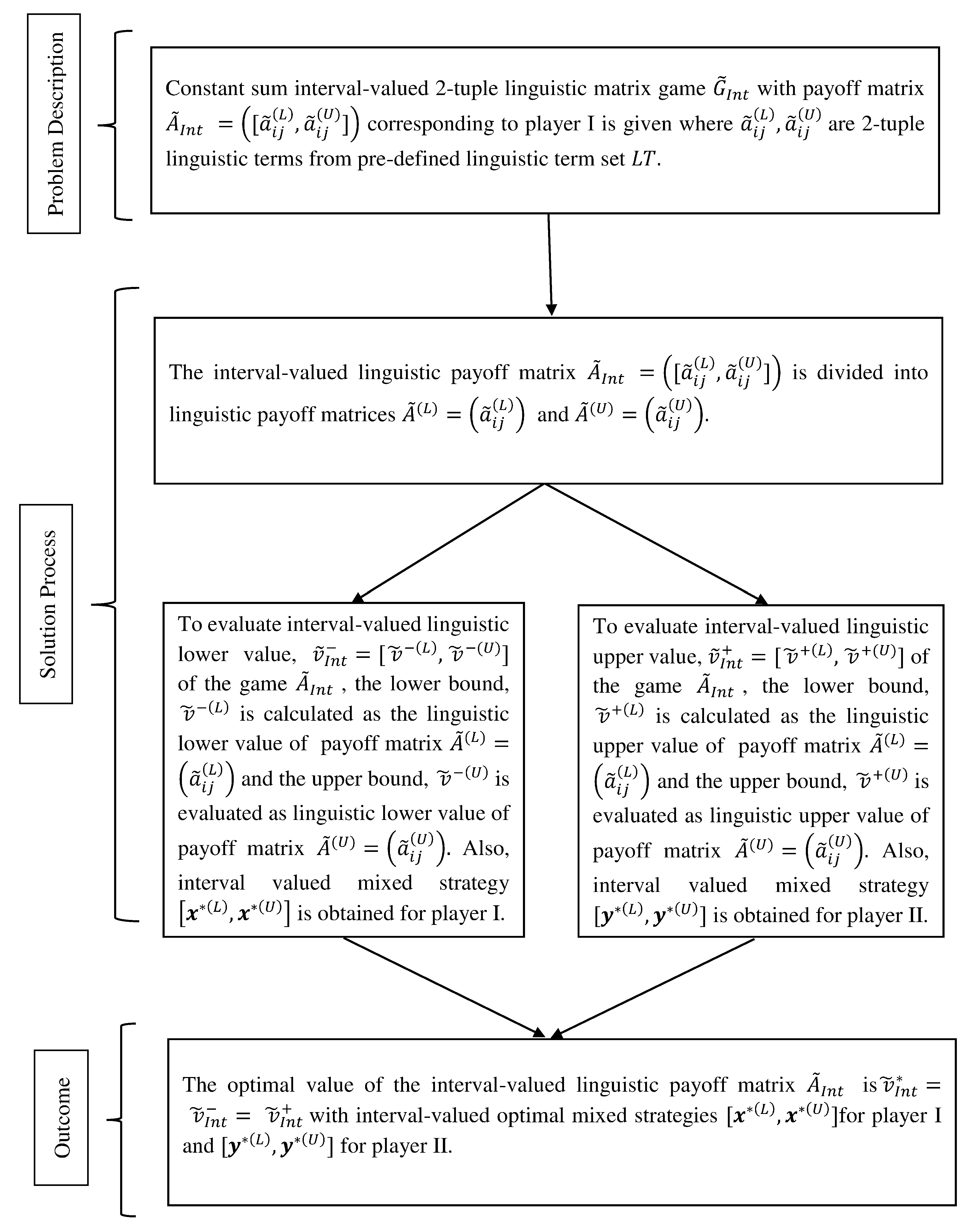
The above algorithm to solve the interval-valued 2-tuple linguistic matrix game can be summarized using the following flowchart.

5. Illustrations and Result Analysis

The game theory has a wide variety of applications in finances, management, and decision sciences. It is also engaged in the real world competing and strategic interactions among players. The interval-valued 2-tuple linguistic game theory facilitates the situations where the range of the payoffs needs to be assessed through subjective thinking of the human mind. For example, the proposed algorithm can be adopted to estimate the market share if two competing companies need to launch their products with different advertising strategies as discussed in Example 1. Now, we present some hypothetical examples to illustrate the validity of the proposed methodology. Herein the examples considered are hypothetical and data is populated synthetically. However, it is not hard to implement these thoughts on real data.

Example 3.

Consider the constant-sum interval-valued linguistic matrix game with interval payoffs from the predefined linguistic term set $LT=\{{\ell }_0:VeryPoor(VP),{\ell }_1:Poor(P),{\ell }_2:ModeratelyPoor(MP),{\ell }_3:Fair(F),{\ell }_4:ModeratelyGood(MG),{\ell }_5:Good(G),{\ell }_6:VeryGood(VG)\}$ with payoff matrix,

$$\begin{array}{c}\hfill {\tilde{A}}_{Int}=\left(\left.\begin{array}{cc}[(G,0.1818),VG]& [(MP,0.1818),(MG,0.2545)]\\ [VP,(P,0.0909)]& [(G,0.4545),VG]\end{array}\right).\right.\end{array}$$

Here,

$$\begin{array}{c}\hfill {\tilde{A}}^{(L)}=\left[\left.\begin{array}{cc}(G,0.1818)& (MP,0.1818)\\ VP& (G,0.4545)\end{array}\right]\right.and{\tilde{A}}^{(U)}=\left[\left.\begin{array}{cc}VG& (MG,0.2545)\\ (P,0.0909)& VG\end{array}\right].\right.\end{array}$$

Suppose the mixed strategies for player I be ${\mathbf{x}}^{(L)}=(x_1^{(L)},x_2^{(L)}),x_i^{(L)}\ge 0,i=1,2,{\sum }_{i=1}^2{x}_i^{(L)}=1,$ and ${\mathbf{x}}^{(U)}=(x_1^{(U)},x_2^{(U)}),x_i^{(U)}\ge 0,i=1,2,{\sum }_{i=1}^2{x}_i^{(U)}=1$ for ${\tilde{A}}^{(L)}$ and ${\tilde{A}}^{(U)},$ respectively. In addition, the mixed strategies for player II for linguistic payoff matrix ${\tilde{A}}^{(L)}$ and ${\tilde{A}}^{(U)}$ are defined as ${\mathbf{y}}^{(L)}=(y_1^{(L)},y_2^{(L)}),y_j^{(L)}\ge 0,j=1,2,{\sum }_{j=1}^2{y}_j^{(L)}=1,$ and ${\mathbf{y}}^{(U)}=(y_1^{(U)},y_2^{(U)}),y_j^{(U)}\ge 0,j=1,2,{\sum }_{j=1}^2{y}_j^{(U)}=1.$

In view of the approach proposed in the paper, construct model (M3) to obtain the lower bound of the interval-valued linguistic lower value ${\tilde{v}}_{Int}^{-}$ of the game with payoff matrix ${\tilde{A}}_{Int}.$ The formulated LLP problem is as follows:

$$\begin{array}{c}\max \begin{array}{c}{\tilde{v}}^{-(L)}\hfill \end{array}\hfill \\ subjectto\hfill \\ ({\ell }_5,0.1818)x_1^{(L)}\oplus ({\ell }_0,0)x_2^{(L)}\ge {\tilde{v}}^{-(L)},\hfill \\ ({\ell }_2,0.1818)x_1^{(L)}\oplus ({\ell }_5,0.4545)x_2^{(L)}\ge {\tilde{v}}^{-(L)},\hfill \\ x_1^{(L)}+x_2^{(L)}=1,\hfill \\ x_1^{(L)},x_2^{(L)}\ge 0.\hfill \end{array}$$

The above formulation can be converted into a linear programming problem in view of model (M4):

$$\begin{array}{c}\min V^{(L)}=\begin{array}{c}{X}_1^{(L)}+X_2^{(L)},\hfill \end{array}\hfill \\ subjectto\hfill \\ 5.1818X_1^{(L)}+0X_2^{(L)}\ge 1,\hfill \\ 2.1818X_1^{(L)}+5.4545X_2^{(L)}+\ge 1,\hfill \\ X_1^{(L)},X_2^{(L)}\ge 0.\hfill \end{array}$$

Similarly, the corresponding model for evaluating upper bound of gain-floor of player I can be constructed using model (M6):

$$\begin{array}{c}\min V^{(U)}=\begin{array}{c}{X}_1^{(U)}+X_2^{(U)},\hfill \end{array}\hfill \\ subjectto\hfill \\ 6X_1^{(U)}+1.0909X_2^{(U)}\ge 1,\hfill \\ 4.2545X_1^{(U)}+6X_2^{(U)}\ge 1,\hfill \\ X_1^{(U)},X_2^{(U)}\ge 0.\hfill \end{array}$$

The optimal solutions of the above problems are $({X_1^{(L)}}^{*}=0.193,{X_2^{(L)}}^{*}=0.1061),$ with optimal value ${V^{(L)}}^{*}=0.2991$ and $({X_1^{(U)}}^{*}=0.1565,{X_2^{(U)}}^{*}=0.0557)$ with optimal value ${V^{(U)}}^{*}=0.2123$.

Hence, for player I, the interval-valued linguistic gain-floor is ${\tilde{v}}_{Int}^{{-}^{*}}=[({\ell }_3,0.3434),({\ell }_5,-0.2897)]$ with optimal mixed strategies $([0.6453,0.7372],[0.2624,0.3547])$. The interval-valued optimal mixed strategies suggest that the probability for choosing the strategies lie in the evaluated intervals such that the sum is 1.

Likewise, the interval-valued loss ceiling of player II can be obtained using the LLP models (M7) and (M8). The corresponding transformed LPP models are as follows:

$$\begin{array}{c}\max V^{(L)}=\begin{array}{c}{Y}_1^{(L)}+Y_2^{(L)},\hfill \end{array}\hfill \\ subjectto\hfill \\ 5.1818Y_1^{(L)}+2.1818Y_2^{(L)}\le 1,\hfill \\ 0Y_1^{(L)}+5.4545Y_2^{(L)}\le 1,\hfill \\ Y_1^{(L)},Y_2^{(L)}\ge 0,\hfill \end{array}$$

and

$$\begin{array}{c}\max V^{(U)}=\begin{array}{c}{Y}_1^{(U)}+Y_2^{(U)},\hfill \end{array}\hfill \\ subjectto\hfill \\ 6Y_1^{(U)}+4.2545Y_2^{(U)}\le 1,\hfill \\ 1.0909Y_1^{(U)}+6Y_2^{(U)}\le 1,\hfill \\ Y_1^{(U)},Y_2^{(U)}\ge 0.\hfill \end{array}$$

The optimal solutions are $({Y_1^{(L)}}^{*}=0.1158,{Y_2^{(L)}}^{*}=0.1833)$ and $({Y_1^{(U)}}^{*}=0.0557,{Y_2^{(U)}}^{*}=0.1565)$ with the optimal values as ${V^{(L)}}^{*}=0.2991$ and ${V^{(U)}}^{*}=0.2122$, respectively.

It results in optimal strategy as $([0.2624,0.3872],[0.6128,0.7372])$ with loss-ceiling as ${\tilde{v}}_{Int}^{{+}^{*}}=[({\ell }_3,0.3434),({\ell }_5,-0.2897)].$

Hence, interval-valued linguistic value of the game ${\tilde{G}}_{Int}$ is ${\tilde{v}}_{Int}^{*}=[({\ell }_3,0.3434),({\ell }_5,-0.2897)].$

Now, we present another example to demonstrate the applicability of the methodology to the problems with more than two strategies.

Example 4.

Consider the constant-sum interval-valued linguistic matrix game with interval payoffs from the predefined linguistic term set $LT=\{{\ell }_0:VeryPoor(VP),{\ell }_1:Poor(P),{\ell }_2:ModeratelyPoor(MP),{\ell }_3:Fair(F),{\ell }_4:ModeratelyGood(MG),{\ell }_5:Good(G),{\ell }_6:VeryGood(VG)\}$ with payoff matrix,

$$\begin{array}{c}\hfill {\tilde{A}}_{Int}=\left(\left.\begin{array}{ccccc}[F,G]& [(MG,-0.5),G]& [MP,MG]& [MP,MG]& [MG,G]\\ [F,(G,-0.3)]& [MP,F]& [G,VG]& [F,G]& VP\\ [F,MG]& [(G,0.2),VG]& [F,G]& [F,G]& [MP,(G,-0.2)]\end{array}\right).\right.\end{array}$$

Here,

$$\begin{array}{c}\hfill {\tilde{A}}^{(L)}=\left[\left.\begin{array}{ccccc}F& (MG,-0.5)& MP& MP& MG\\ F& MP& G& F& VP\\ F& (G,0.2)& F& F& MP\end{array}\right]\right.and{\tilde{A}}^{(U)}=\left[\left.\begin{array}{ccccc}G& G& MG& MG& G\\ (G,-0.3)& F& VG& G& VP\\ MG& VG& G& G& (G,-0.2)\end{array}\right].\right.\end{array}$$

Suppose the mixed strategies for player I be ${\mathbf{x}}^{(L)}=(x_1^{(L)},x_2^{(L)},x_3^{(L)}),x_i^{(L)}\ge 0,i=1,\dots ,3,{\sum }_{i=1}^3{x}_i^{(L)}=1,$ and ${\mathbf{x}}^{(U)}=(x_1^{(U)},x_2^{(U)},x_3^{(U)}),x_i^{(U)}\ge 0,i=1,\dots ,3,{\sum }_{i=1}^3{x}_i^{(U)}=1$ for ${\tilde{A}}^{(L)}$ and ${\tilde{A}}^{(U)},$ respectively. In addition, the mixed strategies for player II for linguistic payoff matrix ${\tilde{A}}^{(L)}$ and ${\tilde{A}}^{(U)}$ are defined as ${\mathbf{y}}^{(L)}=(y_1^{(L)},y_2^{(L)},y_3^{(L)},y_4^{(L)},y_5^{(L)}),y_j^{(L)}\ge 0,j=1,\dots ,5,{\sum }_{j=1}^5{y}_j^{(L)}=1,$ and ${\mathbf{y}}^{(U)}=(y_1^{(U)},y_2^{(U)},y_3^{(U)},y_4^{(U)},y_5^{(U)}),y_j^{(U)}\ge 0,j=1,\dots ,5,{\sum }_{j=1}^5{y}_j^{(U)}=1.$

In view of the approach proposed in the paper, construct model (M3) to obtain the lower bound of the interval-valued linguistic lower value ${\tilde{v}}_{Int}^{-}$ of the game with payoff matrix ${\tilde{A}}_{Int}.$ The formulated LLP problem is as follows:

$$\begin{array}{c}\max \begin{array}{c}{\tilde{v}}^{-(L)}\hfill \end{array}\hfill \\ subjectto\hfill \\ ({\ell }_3,0)x_1^{(L)}\oplus ({\ell }_3,0)x_2^{(L)}\oplus ({\ell }_3,0)x_3^{(L)}\ge {\tilde{v}}^{-(L)},\hfill \\ ({\ell }_4,-0.5)x_1^{(L)}\oplus ({\ell }_2,0)x_2^{(L)}\oplus ({\ell }_5,0.2)x_3^{(L)}\ge {\tilde{v}}^{-(L)},\hfill \\ ({\ell }_2,0)x_1^{(L)}\oplus ({\ell }_5,0)x_2^{(L)}\oplus ({\ell }_3,0)x_3^{(L)}\ge {\tilde{v}}^{-(L)},\hfill \\ ({\ell }_2,0)x_1^{(L)}\oplus ({\ell }_3,0)x_2^{(L)}\oplus ({\ell }_3,0)x_3^{(L)}\ge {\tilde{v}}^{-(L)},\hfill \\ ({\ell }_4,0)x_1^{(L)}\oplus ({\ell }_0,0)x_2^{(L)}\oplus ({\ell }_2,0)x_3^{(L)}\ge {\tilde{v}}^{-(L)},\hfill \\ x_1^{(L)}+x_2^{(L)}+\dots +x_n^{(L)}=1,\hfill \\ x_1^{(L)},x_2^{(L)},\dots ,x_n^{(L)}\ge 0.\hfill \end{array}$$

The above formulation can be converted into a linear programming problem in view of model (M4)

$$\begin{array}{c}\min V^{(L)}=\begin{array}{c}{X}_1^{(L)}+X_2^{(L)}+X_3^{(L)},\hfill \end{array}\hfill \\ subjectto\hfill \\ 3X_1^{(L)}+3X_2^{(L)}+3X_3^{(L)}\ge 1,\hfill \\ 3.5X_1^{(L)}+2X_2^{(L)}+5.2X_3^{(L)}\ge 1,\hfill \\ 2X_1^{(L)}+5X_2^{(L)}+3X_3^{(L)}\ge 1,\hfill \\ 2X_1^{(L)}+3X_2^{(L)}+3X_3^{(L)}\ge 1,\hfill \\ 4X_1^{(L)}+0X_2^{(L)}+2X_3^{(L)}\ge 1,\hfill \\ X_1^{(L)},X_2^{(L)},X_3^{(L)}\ge 0.\hfill \end{array}$$

Similarly, the corresponding model for evaluating upper bound of gain-floor of player I can be constructed using model (M6):

$$\begin{array}{c}\min V^{(U)}=\begin{array}{c}{X}_1^{(U)}+X_2^{(U)}+X_3^{(U)},\hfill \end{array}\hfill \\ subjectto\hfill \\ 5X_1^{(U)}+4.7X_2^{(U)}+4X_3^{(U)}\ge 1,\hfill \\ 5X_1^{(U)}+3X_2^{(U)}+6X_3^{(U)}\ge 1,\hfill \\ 4X_1^{(U)}+6X_2^{(U)}+5X_3^{(U)}\ge 1,\hfill \\ 4X_1^{(U)}+5X_2^{(U)}+5X_3^{(U)}\ge 1,\hfill \\ 5X_1^{(U)}+0X_2^{(U)}+4.8X_3^{(U)}\ge 1,\hfill \\ X_1^{(U)},X_2^{(U)},X_3^{(U)}\ge 0.\hfill \end{array}$$

The optimal solutions of the above problems are $({X_1^{(L)}}^{*}=0.125,{X_2^{(L)}}^{*}=0,{X_3^{(L)}}^{*}=0.25)$ with optimal value ${V^{(L)}}^{*}=0.375$ and $({X_1^{(U)}}^{*}=0.105,{X_2^{(U)}}^{*}=0.017,{X_3^{(U)}}^{*}=0.099)$ with optimal value ${V^{(U)}}^{*}=0.221$.

Hence, for player I, the interval-valued linguistic gain-floor is ${\tilde{v}}_{Int}^{{-}^{*}}=[({\ell }_3,-0.3334),({\ell }_5,-0.4752)]$ with optimal mixed strategies $([0.3334,0.4751],[0,0.0769],[0.448,0.6667])$.

Likewise, the interval-valued loss ceiling of player II can be obtained using the LLP models (M7) and (M8). The corresponding transformed LPP models are as follows:

$$\begin{array}{c}\max V^{(L)}=\begin{array}{c}{Y}_1^{(L)}+Y_2^{(L)}+Y_3^{(L)}+Y_4^{(L)}+Y_5^{(L)},\hfill \end{array}\hfill \\ subjectto\hfill \\ 3Y_1^{(L)}+3.5Y_2^{(L)}+2Y_3^{(L)}+2Y_4^{(L)}+4Y_5^{(L)}\le 1,\hfill \\ 3Y_1^{(L)}+2Y_2^{(L)}+5Y_3^{(L)}+3Y_4^{(L)}+0Y_5^{(L)}\le 1,\hfill \\ 3Y_1^{(L)}+5.2Y_2^{(L)}+3Y_3^{(L)}+3Y_4^{(L)}+2Y_5^{(L)}\le 1,\hfill \\ Y_1^{(L)},Y_2^{(L)},Y_3^{(L)},Y_4^{(L)},Y_5^{(L)}\ge 0,\hfill \end{array}$$

and

$$\begin{array}{c}\max V^{(U)}=\begin{array}{c}{Y}_1^{(U)}+Y_2^{(U)}+Y_3^{(U)}+Y_4^{(U)}+Y_5^{(U)},\hfill \end{array}\hfill \\ subjectto\hfill \\ 5Y_1^{(U)}+5Y_2^{(U)}+4Y_3^{(U)}+4Y_4^{(U)}+5Y_5^{(U)}\le 1,\hfill \\ 4.7Y_1^{(U)}+3Y_2^{(U)}+6Y_3^{(U)}+5Y_4^{(U)}+0Y_5^{(U)}\le 1,\hfill \\ 4Y_1^{(U)}+6Y_2^{(U)}+5Y_3^{(U)}+5Y_4^{(U)}+4.8Y_5^{(U)}\le 1,\hfill \\ Y_1^{(U)},Y_2^{(U)},Y_3^{(U)},Y_4^{(U)},Y_5^{(U)}\ge 0.\hfill \end{array}$$

The optimal solutions are $({Y_1^{(L)}}^{*}=0,{Y_2^{(L)}}^{*}=0,{Y_3^{(L)}}^{*}=0,{Y_4^{(L)}}^{*}=0.25,{Y_5^{(L)}}^{*}=0.125)$ and $({Y_1^{(U)}}^{*}=0.1016,{Y_2^{(U)}}^{*}=0,{Y_3^{(U)}}^{*}=0,{Y_4^{(U)}}^{*}=0.1045,{Y_5^{(U)}}^{*}=0.0148)$ with the optimal values as ${V^{(L)}}^{*}=0.375$ and ${V^{(U)}}^{*}=0.221$, respectively.

It results in optimal strategy as $([0,0.4597],0,0,[0.4728,0.6667],[0.067,0.3334])$ with loss-ceiling as ${\tilde{v}}_{Int}^{{+}^{*}}=[({\ell }_3,-0.3334),({\ell }_5,-0.4752)].$ For the strategies for which the optimal value is 0, it depicts that the player will never choose those strategies to maximize his/her payoff.

Hence, interval-valued linguistic value of the game ${\tilde{G}}_{Int}$ is ${\tilde{v}}_{Int}^{*}=[({\ell }_3,-0.3334),({\ell }_5,-0.4752)].$

Note 1: It is noteworthy that in Example 2 of [17], the considered linguistic payoff matrix $\tilde{A}$ is a particular matrix of ${\tilde{A}}_{Int}$ i.e., each ${\tilde{a}}_{ij}\in [{\tilde{a}}_{ij}^{(L)},{\tilde{a}}_{ij}^{(U)}];i=1,2,3,j=1,\dots ,5.$ In addition, the linguistic value of the game, ${\tilde{v}}^{*}=({\ell }_4,-0.3343)\in [({\ell }_3,-0.3334),({\ell }_5,-0.4752)],$ but the optimal mixed strategy for both players corresponding to some strategies do not belong in the acquired intervals.

6. Conclusions

In this paper, a two-player constant-sum interval-valued 2-tuple linguistic matrix game is defined and analyzed to acquire the mixed strategies and value of the game for players I and II. The interval linguistic matrix game is split into two linguistic matrix games to evaluate the value of the game in interval form. The linguistic linear programming is then adopted to solve each linguistic matrix game. A flowchart to summarize the algorithm is also given. In the suggested approach, the value of the game maintains the form of interval-valued linguistic variables, but the mixed strategies for each player are not in interval form. The methodology shows promising results in the game problems where the payoffs to the given strategies of two-players are not numerical or linguistic variables but interval-valued linguistic information. In this approach, we obtain two linguistic matrices from the given interval-valued linguistic payoff matrix. We envision that the interval linear programming can be adopted as the alternative approach to solve such class of game that results in the interval-valued linguistic value of the game as well as the mixed strategies also appearing as an interval. In addition, the bimatrix games with interval-valued linguistic payoff matrix can be explored in the future to enhance the applicability of game theory in this uncertain world.

References

- Neumann, J.V.; Morgenstern, O. Theory of Games and Economic Behavior; Princeton University Press: New York, NY, USA, 1994. [Google Scholar]
- Campos, L. Fuzzy linear programming to solve fuzzy matrix games. Fuzzy Sets Syst. 1989, 32, 275–289. [Google Scholar] [CrossRef]
- Bector, C.R.; Chandra, S. Fuzzy Mathematical Programming and Fuzzy Matrix Games; Springer: Berlin, Germany, 2005. [Google Scholar]
- Nishizaki, I.; Sakawa, M. Fuzzy and Multiobjective Games for Conflict Resolution; Physica-Verlag: Heidelberg, Germany, 2001. [Google Scholar]
- Avsar, Z.M.; Gursoy, M.B. A note on two-person zero-sum communicating stochastic games. Oper. Res. Lett. 2006, 34, 412–420. [Google Scholar] [CrossRef] [Green Version]
- Kurano, M.; Yasuda, M.; Nakagami, J.I.; Yoshida, Y. An Interval Matrix Game and Its Extensions to Fuzzy and Stochastic Games. Available online: http://www.math.s.chiba-u.ac.jp/~yasuda/accept/SIG2.pdf (accessed on 5 June 2018).
- Collins, W.D.; Hu, C.-Y. Fuzzily determined interval matrix games. In Proceedings of the Biscse 2005, Berkeley, CA, USA, 2–5 November 2005; Available online: http://www-bisc.cs.berkeley.edu/BISCSE2005/Abstracts-Proceeding/Friday/FM3/Chenyi-Hu.pdf (accessed on 9 June 2018).
- Collins, W.D.; Hu, C.-Y. Studying interval-valued matrix games with fuzzy logic. Soft Comput. 2008, 12, 147–155. [Google Scholar] [CrossRef]
- Hladik, M. Interval valued bimatrix games. Kybernetika 2010, 46, 435–446. [Google Scholar]
- Liu, S.-T.; Kao, C. Matrix games with interval data. Comput. Ind. Eng. 2010, 56, 1697–1700. [Google Scholar] [CrossRef]
- Shashikhin, V.N. Antagonistic game with interval payoff functions. Cybern. Syst. Anal. 2004, 40, 556–564. [Google Scholar] [CrossRef]
- Collins, W.D.; Hu, C.-Y. Interval matrix games. In Knowledge Processing with Interval and Soft Computing; Hu, C.-Y., Ed.; Springer: London, UK, 2008; Chapter 7; pp. 1–19. [Google Scholar]
- Li, D.-F.; Nan, J.-X.; Zhang, M.-J. Interval programming models for matrix games with interval payoffs. Optim. Methods Softw. 2010, 27, 1–16. [Google Scholar] [CrossRef]
- Li, D.-F. Linear programming approach to solve interval-valued matrix games. Omega 2011, 39, 655–666. [Google Scholar] [CrossRef]
- Arfi, B. Linguistic fuzzy-logic game theory. J. Confl. Resolut. 2006, 50, 28–57. [Google Scholar] [CrossRef]
- Arfi, B. Linguistic fuzzy-logic social game of cooperation. Ration. Soc. 2006, 18, 471–537. [Google Scholar] [CrossRef]
- Singh, A.; Gupta, A.; Mehra, A. Matrix Games with 2-tuple Linguistic Information. Ann. Oper. Res. 2018. [Google Scholar] [CrossRef]
- Herrera, F.; Martinez, L. A 2-tuple fuzzy linguistic representation model for computing with words. IEEE Trans. Fuzzy Syst. 2000, 8, 746–752. [Google Scholar]
- Balezentis, A.; Balezentis, T. A novel method for group multi-attribute decision making with two-tuple linguistic computing: Supplier evaluation under uncertainty. Econ. Comput. Econ. Cybern. Stud. Res. 2011, 4, 5–30. [Google Scholar]
- Wei, G.W. A method for multiple attribute group decision making based on the ET-WG and ET-OWG operators with 2-tuple linguistic information. Exp. Syst. Appl. 2010, 37, 7895–7900. [Google Scholar] [CrossRef]
- Zhang, H. The multiattribute group decision making method based on aggregation operators with interval-valued 2-tuple linguistic information. Math. Comput. Model. 2012, 56, 27–35. [Google Scholar] [CrossRef]
- Liu, H.-C.; Liu, L.; Wuc, J. Material selection using an interval 2-tuple linguistic VIKOR method considering subjective and objective weights. Mater. Des. 2013, 52, 158–167. [Google Scholar] [CrossRef]
- You, X.-Y.; You, J.-X.; Liu, H.-C.; Zhen, L. Group multi-criteria supplier selection using an extended VIKOR method with interval 2-tuple linguistic information. Exp. Syst. Appl. 2015, 42, 1906–1916. [Google Scholar] [CrossRef]
- Singh, A.; Gupta, A.; Mehra, A. An AHP-Promethee II method for 2-tuple linguistic multicriteria group decision making. In Proceedings of the 2015 4th International Conference on Reliability, Infocom Technologies and Optimization (ICRITO) (Trends and Future Directions), Noida, India, 2–4 September 2015. [Google Scholar] [CrossRef]
Figure 1.
Proposed methodology.
© 2018 by the authors. Licensee MDPI, Basel, Switzerland. This article is an open access article distributed under the terms and conditions of the Creative Commons Attribution (CC BY) license (http://creativecommons.org/licenses/by/4.0/).
Share and Cite
MDPI and ACS Style
Singh, A.; Gupta, A. Matrix Games with Interval-Valued 2-Tuple Linguistic Information. Games 2018, 9, 62. https://doi.org/10.3390/g9030062
AMA Style
Singh A, Gupta A. Matrix Games with Interval-Valued 2-Tuple Linguistic Information. Games. 2018; 9(3):62. https://doi.org/10.3390/g9030062
Chicago/Turabian StyleSingh, Anjali, and Anjana Gupta. 2018. "Matrix Games with Interval-Valued 2-Tuple Linguistic Information" Games 9, no. 3: 62. https://doi.org/10.3390/g9030062
Note that from the first issue of 2016, this journal uses article numbers instead of page numbers. See further details here.