Critical Discount Factor Values in Discounted Supergames


Department of Mathematics and Systems Analysis, Aalto University School of Science, P.O. Box 11100, FI-00076 Aalto, Finland
*
Author to whom correspondence should be addressed.
Games 2018, 9(3), 47; https://doi.org/10.3390/g9030047
Submission received: 5 June 2018
/
Revised: 27 June 2018
/
Accepted: 6 July 2018
/
Published: 10 July 2018
Abstract
:This paper examines the subgame-perfect equilibria in symmetric supergames. We solve the smallest discount factor value for which the players obtain all the feasible and individually rational payoffs as equilibrium payoffs. We show that the critical discount factor values are not that high in many games and they generally depend on how large the payoff set is compared to the set of feasible payoffs. We analyze how the stage-game payoffs affect the required level of patience and organize the games into groups based on similar behavior. We study how the different strategies affect the set of equilibria by comparing pure, mixed and correlated strategies. This helps us understand better how discounting affects the set of equilibria and we can identify the games where extreme patience is required and the type of payoffs that are difficult to obtain. We also observe discontinuities in the critical values, which means that small changes in the stage-game payoffs may affect dramatically the equilibrium payoffs.
Keywords:
repeated game; folk theorem; discount factor; 2 × 2 games; payoff set; correlated equilibriumMSC:
91A20JEL Classification:
C731. Introduction
The folk theorem tells us that any feasible and individually rational (FIR) payoff is an equilibrium, when the players are patient enough [1,2,3,4]. However, the players may not be extremely patient but they rather have some intermediate value for the discount factor. This paper finds the smallest discount factor value for which the FIR payoffs are the equilibrium payoffs in the symmetric supergames. This extends the folk theorem by solving exactly how patient the players need to be as a function of the stage-game payoffs. This reveals why and in what type of games extreme patience is required in the folk theorem and what payoffs are difficult to obtain.
This paper compares three types of strategies: pure strategies with and without public correlation and mixed strategies without public correlation. We want to examine how these assumptions affect the results. In some applications, it may be reasonable to assume that the players may only use pure strategies and they may not be able to coordinate their actions using a correlation device. The pure-strategy model has been examined in [5,6,7,8]. These papers characterize the subgame-perfect equilibria with a set-valued fixed-point equation, which forms the basis of our analysis. The mixed-strategy model has been studied in the more general model of imperfect public monitoring [9,10,11]; see also [12,13] for the model examined in this paper.
The computation of the payoff set has been examined in [14,15,16,17,18]. These papers assume public correlation, which makes the payoff set convex and simplifies the computation dramatically. References [19,20] have developed a method for computing pure-strategy equilibria without public correlation.
The main result of this paper is to solve the critical values, i.e., the smallest discount factor value for which the players obtain all the FIR payoffs as equilibrium payoffs. The results are based on solving analytically and geometrically the fixed-point equation of [7,8]. This idea has been presented in [21] where the critical values are solved in a class of prisoner’s dilemma games under public randomization; see also Sections 2.5.3 and 2.5.6 in [11]. The pure-strategy model without public correlation is a quite straightforward extension of [21], but the mixed-strategy model requires analyzing totally new types of strategies with complicated payoffs; see [12,13]. We restrict our analysis to the symmetric games since the set of pure-strategy equilibria may be empty in asymmetric games, it may be difficult to find the smallest equilibrium payoffs [22], and it is tedious to examine all the asymmetric games.
The results of this paper can be used (i) to identify the games where the players have trouble in obtaining all the payoffs and to find the payoffs that are difficult to obtain, (ii) to understand better how the equilibrium payoffs depend on the discount factor, and (iii) to find a range of discount factor values for which the computation of equilibria is easy. For example, we know that the payoff set coincides with the FIR payoffs for all the discount factor values above the critical value, and there is no need to compute the payoff set for these values. We also observe discontinuities in the critical values, which means that the set of equilibria may not behave well, i.e., small changes in the stage-game payoffs may affect dramatically the payoff set.
We organize the games into groups based on the equations that determine the critical values and provide a useful visualization of the critical values in different games. From the figures, it is easy to see when the high level of patience is needed and to make the comparison between the different strategies.
2. The Repeated Game
2.1. Stage Games
In a repeated game, a stage game is played again and again by the same players. A stage game is defined by a finite set of players , a finite set of pure actions for each player , , and the players’ utilities for each action profile , where is the set of pure-action profiles. Moreover, a pure action of player i is denoted and a pure-action profile is .
Each player may randomize over his pure actions . This defines a mixed action such that for each and . The set of probability distributions over is denoted and . A mixed-action profile is denoted by . A support of a mixed action is the set of pure actions that is played with a strictly positive probability: . We also define , and for each , we let be the probability that the action profile a is realized if the mixed-action profile q is played: . In pure strategies, we make the restriction that for one action .
In a model with public correlation, the players observe a realization of a public lottery and they can condition their action based on the signal . For example, two players may agree to take action if and otherwise. This way the players can coordinate their actions such that they randomize between the outcomes and , and avoid the outcomes and . The latter outcomes would be realized if standard mixed strategies were used and no public correlation device was available.
The stage-game payoffs are given by function . For example, if the players choose a mixed-action profile , then player i receives an expected payoff of
Let denote player i’s opponents’ actions. Now, an action profile q is a Nash equilibrium in the stage game if no player has a profitable deviation, i.e.,
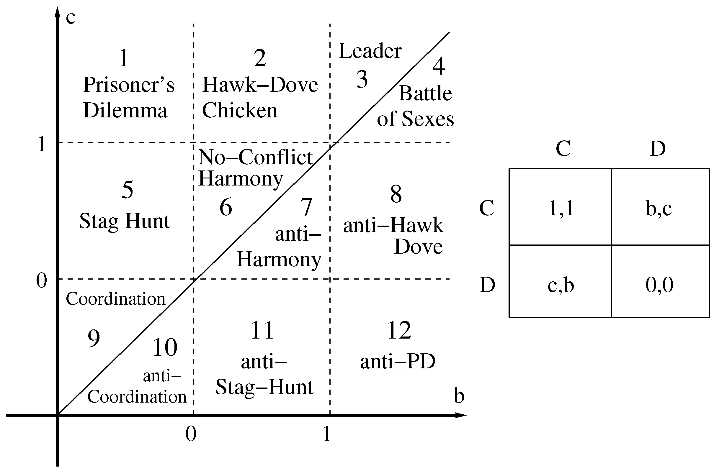
The twelve symmetric strict ordinal games are presented in Figure 1, see ref. [23] for the taxonomy. Strict ordinality means that all of the payoffs must be unequal and there can be no indifferences. The two actions are C (cooperate) and D (defect), and they give the players the payoffs , , and ; the corresponding action profiles are also denoted by letters . For example, if the players choose the action profile , the players receive payoffs and .
2.2. Repeated Games
We examine a model where the stage game is repeated infinitely many times and these games are sometimes called as supergames. We assume that the players observe all the past realized pure actions but not the probabilities that the other players are using in their mixed strategies. The public past play is denoted by the set of histories , where is the empty set and corresponds to the beginning of the game. Thus, the history contains all the pure actions that were played in the previous rounds. The set of all possible histories is . A behavior strategy of player is a mapping that assigns a probability distribution over player i’s pure actions for each possible history . The set of player i’s strategies is . The players’ strategies form a strategy profile , a strategy profile of all players except player i is denoted by and the set of strategy profiles is given by . A pure strategy assigns a pure action for each possible history . With public correlation, the players observe a public signal on each round k before making their decisions, and thus the history contains all the past pure actions, signals and the current signal.
We assume that the players discount the future payoffs with a common discount factor . They have the same discount factor since we examine symmetric games. The expected discounted payoff of a strategy profile to player i is
where is the payoff of player i at round k induced by the strategy profile . A strategy profile is a Nash equilibrium if no player has a profitable deviation, i.e.,
and it is a subgame-perfect equilibrium (SPE) if it induces a Nash equilibrium in every subgame, i.e.,
where is the restriction of the strategy profile after history . From now on, by equilibrium we mean subgame-perfect equilibrium.
2.3. Critical Discount Factor Values
Let V be the compact set of SPE payoffs and we also use when we want to emphasize the players’ discount factor . By , and we refer to the equilibria in pure strategies with and without public correlation, and mixed strategies, respectively.
The player i’s minimum equilibrium payoff, which is also called the punishment payoff, is denoted by , when is non-empty; and this is the case in the symmetric supergames. Similarly, the maximum equilibrium payoff is . The minimax payoff is
Please note that the minimax payoffs can be different in pure and mixed strategies. However, it holds under perfect monitoring that , [4,11]. The player’s minimum and maximum payoffs in a compact set W are denoted by and , respectively. Moreover, is the maximum symmetric payoff in the set W.
Let be the set of feasible payoffs, where denotes the convex hull of the set. The set of feasible and individually rational (FIR) payoffs are
Let us denote the critical discount factor by
which gives the smallest discount factor value when the payoff set coincides with the FIR payoffs. Please note that is convex and thus for all by Theorem 3.
Please note that the minimum equilibrium payoff may be strictly higher than the minimax payoff , and then it is impossible to obtain all the FIR payoffs for given . The minimum pure-strategy payoffs have been studied in [24], and [22] present an algorithm for finding the punishment paths and payoffs.
For most of the symmetric games, the minimum equilibrium payoffs in pure strategies are equal to the minimax payoffs for all discount factors. No conflict, its anti-game and anti-stag hunt games are the only exceptions. In these games, the minimum payoffs are equal to the minimax values when the players are patient enough. This issue does not affect the results, since it can be shown the required levels of patience are smaller than the critical values.
The minimax payoffs in mixed strategies are the same as in pure strategies, except in leader, battle of the sexes, coordination and anti-coordination games. In these games, the minimax payoff is given by a mixed-strategy Nash equilibrium. Thus, for all in mixed strategies. It can be shown that the FIR payoffs are not obtained for any in these games.
2.4. The Characterization of Equilibria
A pair of an action profile and a continuation payoff is admissible with respect to W if it satisfies
This incentive-compatibility condition means that it is better for player i to take action and get the continuation payoff than to deviate and then obtain .
For a set of continuation payoffs W, the set of supportable action profiles is denoted by
For , we denote the set of admissible continuation payoffs as
Let be an affine mapping that corresponds to an action profile and a discount factor
where I is an identity matrix and T is an diagonal matrix with the discount factor on the diagonal. The mapping is also defined for sets; then the addition is the Minkowski sum and . Finally, we denote the admissible payoffs that start with an action profile by .
Theorem 1.
The payoff set under public correlation is given by the largest compact set satisfying [11]
Let us now characterize the set of equilibria in mixed strategies [12,13]. In a repeated game, the play at each round is strategically equivalent to playing an augmented stage game, where the continuation payoffs are included in the payoffs. For each action profile , the payoff in the augmented game is given by
where is the continuation payoff after a. Please note that in pure strategies there are only two continuation payoffs for each player: if the player follows the equilibrium path or if the player deviates. In mixed strategies, there can be a different continuation payoff after each action profile . Let denote the set of Nash equilibrium payoffs in a stage game with payoffs , .
Now, we are ready to state the characterization for the subgame-perfect equilibrium payoffs [12,13]. This result has been derived earlier in a more general model of imperfect monitoring [11].
Theorem 2.
The payoff set is the largest compact fixed point of :
This means that the payoff set corresponds to the set of equilibria in augmented stage games where the payoffs are and each can be chosen from the set .
2.5. Monotonicity and Helpful Results
In this subsection, by we refer to the sets , and , depending on which strategies are in question. A set W is called self-generating if . The following result follows directly from Theorems 1 and 2 and Equation (13).
Proposition 1.
If a bounded set W is self-generating then .
The following shows that the payoff set is monotone in the discount factor when it is convex [8,11,24,25].
Theorem 3.
Suppose is convex then for .
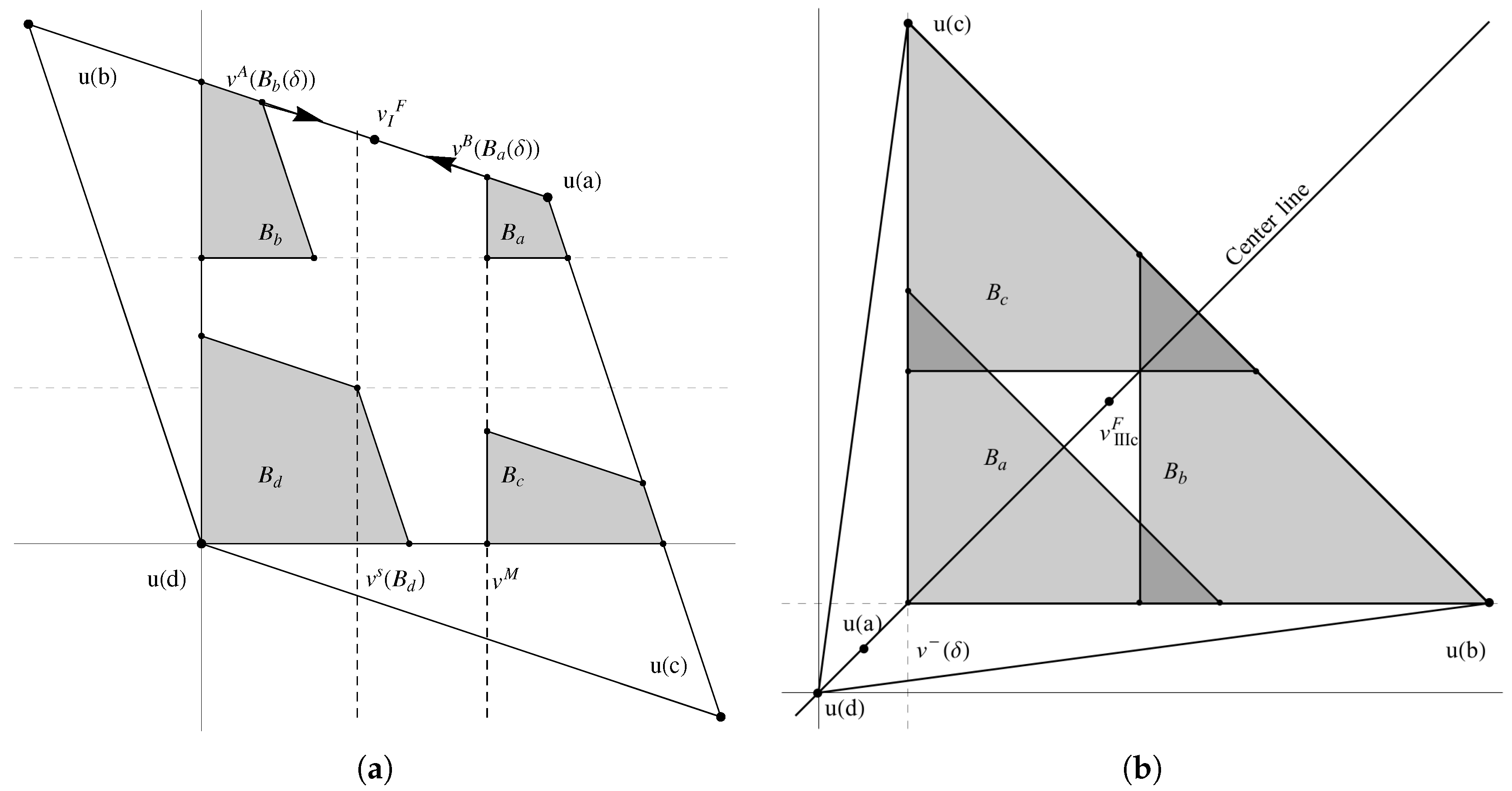
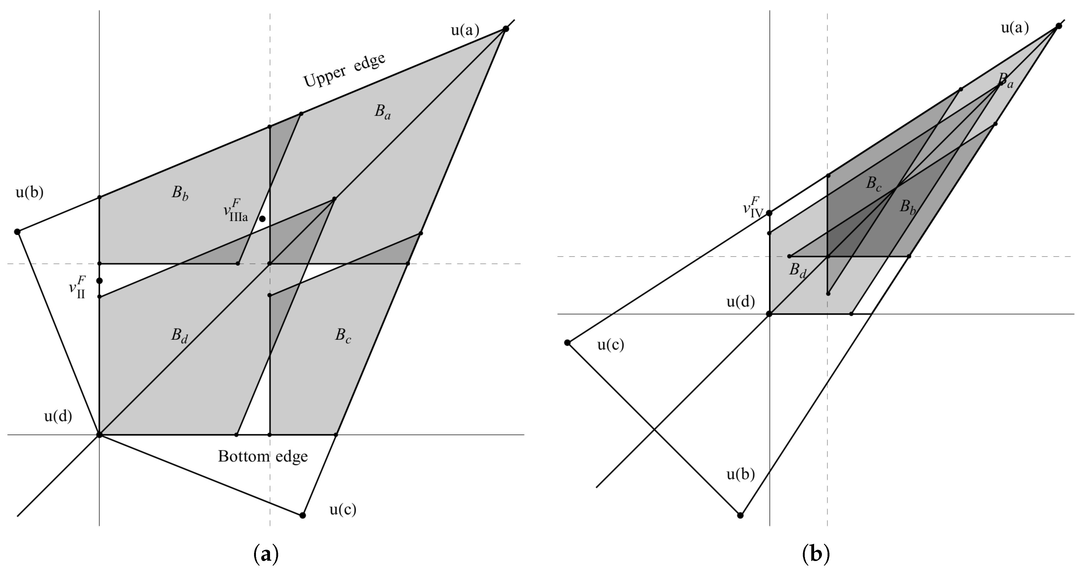
Let , , and be the corners of a quadrilateral set W corresponding to payoffs , , and . For example, if and are the payoffs in the northeast and northwest corners of , then and are the northeast and the northwest corners of the sets and ; see Figure 2a. Moreover, let
This is the right-hand side of Equation (8) for the column that contains the maximum payoff in the game.
Remark 1.
If , , then for all a and i where player i can deviate to the maximum payoff of the stage game.
The following result describes how the sets , , may cover the boundaries of . The result implies that we need as many sets , , to cover the FIR payoffs as there are corner points in .
Proposition 2.
The set , , may only cover the corner point of closest to . It cannot cover the other corner points or the boundary of between these other corner points.
Proof.
By the definition of , the set is contracted by and is thus strictly smaller than . The translation part moves the set towards . ☐
3. Results for Different Strategies
We present now the results for the three different strategies, and the proofs are given in the appendix. Section 4 gives an example of the proofs in a prisoner’s dilemma game. The proofs for the mixed strategies are novel in Appendix C. However, the principle behind the proofs is the same but finding all the mixed-strategy payoffs is more complicated.
The results are based on Theorems 1 and 2 and Equation (13), which tell that the payoff set coincides with the FIR payoffs when the admissible payoffs cover all the payoffs in . To find the critical value , we need to find the smallest discount factor for this to happen. The main idea is to find the last payoff point that is covered when the discount factor is increased to . The value is typically solved from a condition that two sets, say and intersect. In the proofs, we show both the necessary and sufficient conditions for : the point is not covered for a smaller discount factor value and all the other FIR payoffs are covered for the given value .
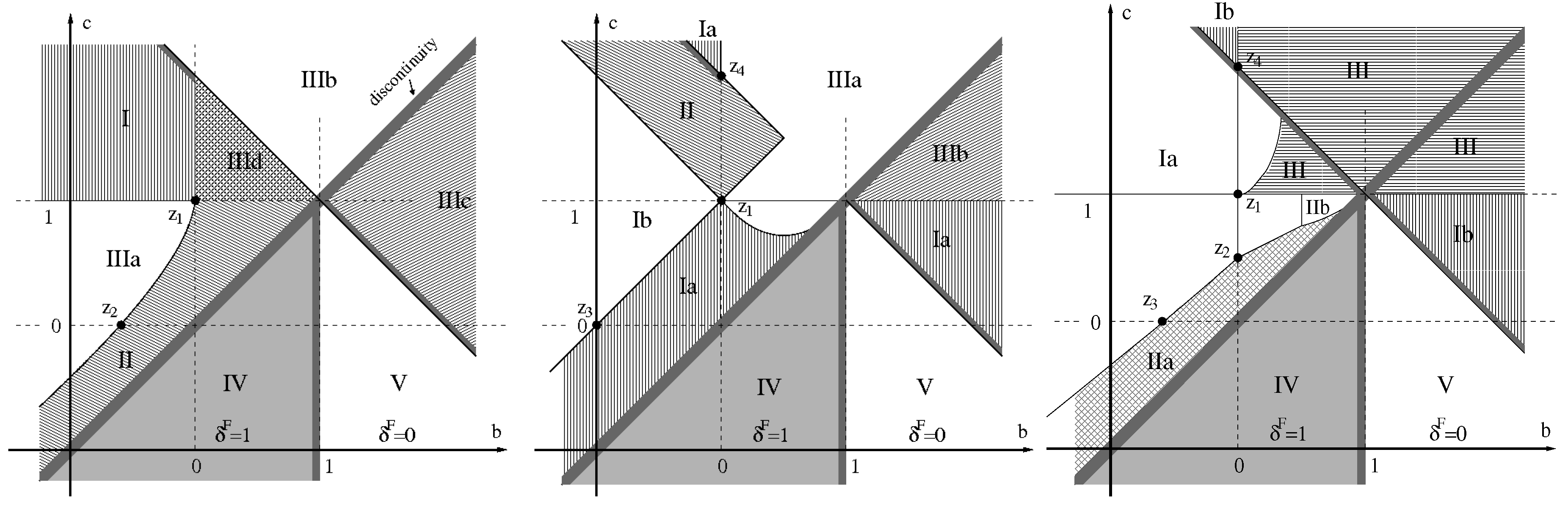
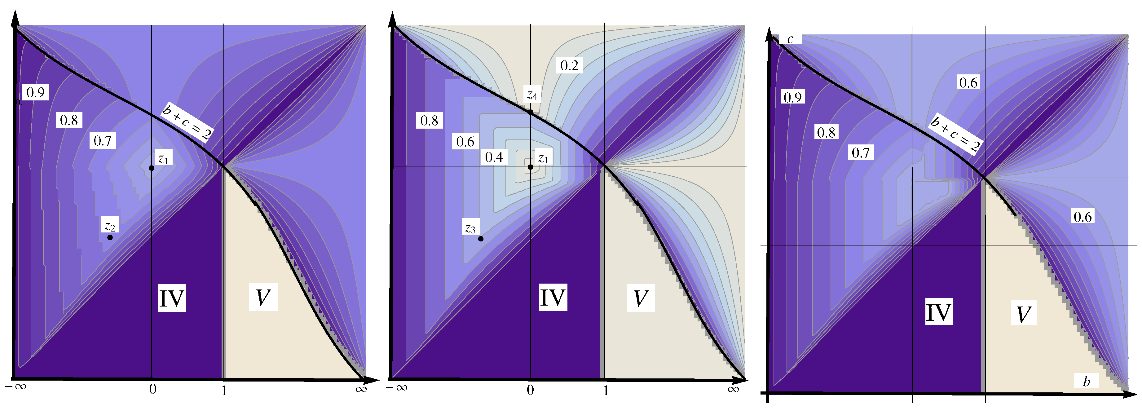
The results are given in Table 1, Table 2 and Table 3. They show the values of for different groups of games. Please note that the group boundaries cross the game boundaries. For example, there are two groups of prisoner’s dilemma (PD) games in pure strategies without public correlation: the quadrilateral PDs belong to Group I (see example in Figure 2a) and the triangle PDs in Group IIIb, and the boundary between these groups is given by the equation . Also, different games may belong to the same group: the triangle PDs and triangle chicken games all belong to Group IIIb. Figure 3 shows the groups for the different strategies. The thick grey lines show that there are discontinuities of between the groups. This means that the value of is not continuous and there may be a jump, when b and c are changed. Figure 4 shows the values of in different games.
The groups are based on the equations that determine the value of and the location of the last payoff . We note that our classification is heuristic, and the games could be organized differently into groups. In pure strategies without public correlation: in Group I, is found on the upper edge of between and , on the bottom edge between and in Group II, and in the middle in Groups IIIa-d. In Group IV, we have and in Group V, .
With public correlation, the groups are based on the last corner point to be covered: in Group I, the last corner is in the northwest, corresponding to or , the corner in Group II, and the corner in Group III.
In mixed strategies, the groups are the following. In Group Ia, the last point to be covered is on the boundary between and , i.e., the intersection of and . Group Ib corresponds to the triangle games, where and intersect. In Group II, a corner point determines the value of : corner is last to be covered in Group IIa and corner in Group IIb. The intersection of and determines the value for Group III.
The overview of the values of is similar for all the strategies. Groups IV and V are the same, and the locations of the high and low values are about the same. However, the values of are much lower with public correlation. The scale with public correlation is between 0 and 1, and between or to 1 with the other strategies. The smallest and the highest values within the game classes are shown with to . The difference between the pure and mixed strategies is surprisingly small; the values are typically smaller than in quadrilateral games and smaller than in triangle games.
We note that for all groups, there are some payoff parameters for which , except in Group V where for all payoffs. For example, when for prisoner’s dilemma, stag hunt and coordination games. This means that we cannot extend the folk theorem unless these extreme payoff parameters can be ruled out.
We can observe that the value of depends on how large is compared to . When is small, it is difficult to play certain actions in the game and the value of is high. For example, it is difficult to play the actions b and c in a prisoner’s dilemma when . Geometrically, this means that stays almost the same but keeps increasing, making the proportion of to smaller. On the other hand, if is large then is smaller. Please note that Groups IV and V are exceptions, where is a constant and thus independent of and .
We also note that there are discontinuities in on some of the group boundaries; see the thick grey lines in Figure 3. The discontinuity means that small changes in the payoffs can affect dramatically the payoff set and how large is. The discontinuity between the prisoner’s dilemma games is surprising and it shows that a small geometric change from the triangle-shape to the quadrangle-shape may affect whether the Pareto efficient payoffs are obtained or not.
For mixed strategies, we have a few remarks. The necessary and sufficient conditions for are more difficult to prove, since the strategies and their payoffs are more complicated. For Groups IIb and III, the values are only upper bounds since we only use the sufficient conditions. In all leader, battle of the sexes, coordination and anti-coordination games, but in the figure we use the values for which the pure-strategy FIR payoffs are obtained as a comparison.
4. Group I in Pure Strategies without Public Correlation
This group is defined by parameters and . These are the prisoner’s dilemmas where is a quadrilateral with an obtuse angle in corner; see Figure 2a. It is enough to examine the upper half of where since is symmetric with respect to the center line. Thus, the last point that is covered is only defined in the upper half of .
The point in Group I is located on the upper edge between and . This point and the corresponding discount factor are solved from the intersection of and . It is enough to consider only player 1’s payoffs:
On the second line, the first payoff can be solved from the right-hand side of the admissibility condition.
We first show that , , if . Since the sets and intersect at , it means that does not belong to either or for . Moreover, the sets and cannot cover on the boundary of by Proposition 2.
Now, let us show that every for some and . We divide into three regions. If then since coincides with for all by Remark 1. If and then we show that . We show that all corner points , and belong to . is the Nash equilibrium and belongs to for any . Also, belongs to if belongs to , because is higher than due to . So for the last corner, we need to show that . It holds that and and the above condition holds if . Using Equation (16), this is equal to and this is true in this group.
Finally, if and then we show that . The corner points are , , and . belongs to trivially by the definition of . since is at the upper edge and covers the edge all the way to . since coincides with for all when by Remark 1. Again, ensures that and thus since .
5. Conclusions
This paper examines the discount factor values for which the subgame-perfect equilibrium payoffs coincide with the FIR payoffs in the symmetric supergames. The main motivation is to study if the folk theorem could be extended in a class of games and find out the reasons why a high level of patience such as is required in some games. We find that the main reason is that it is impossible to obtain payoffs close to the minimax values: (1) this happens in Group IV in all strategies, (2) it is a result of the fact that the mixed-strategy punishment payoff is strictly smaller than the pure-strategy punishment in leader, battle of the sexes, coordination and its anti-game in mixed strategies, and (3) it is due to geometrical reasons in some games, i.e., how the stage-game payoffs are located and how large the FIR payoffs are in proportion to feasible payoffs . If is small, which also means that it is difficult to play certain actions in the game, then a high level of patience is required.
We also examine how the public correlation and the mixed strategies affect the results. The games are organized into a few groups based on the equation that determines the smallest discount factor value as a function of the stage-game payoffs. The groups and the equations are a bit different under different strategies, but the overview looks similar. Even though a lower level of patience is required with public randomization, the highest and the lowest values are obtained in the same regions. The limit is obtained when , when , when and , or in certain anti-games. Thus, it is not possible to extend the folk theorem in any of the typical game classes, such as prisoner’s dilemma, chicken and stag hunt games, unless certain extreme payoffs can be ruled out. Furthermore, the public correlation or mixed strategies do not provide a remedy in these games and it holds that under all strategies.
The results of this paper help in determining the payoff set for high discount factor values. If the discount factor is higher than , then all the FIR payoffs are subgame-perfect equilibrium payoffs. Moreover, it is a bit surprise how small can be with public correlation. It was also observed that there are certain boundaries where is discontinuous, which means that small changes in the payoffs may affect dramatically the equilibrium payoffs.
It should be noted that this kind of analysis could be done in asymmetric games with more than two actions and more than two players. Furthermore, it is left for future research how to compute efficiently all the equilibrium payoffs when the discount factors are smaller than .
Author Contributions
Kimmo Berg is the main author. Markus Kärki calculated the values for and prepared the figures of admissible sets.
Funding
Berg acknowledges funding from Emil Aaltosen Säätiö (Post doc-pooli).
Conflicts of Interest
The authors declare no conflicts of interest.
Appendix A. Pure Strategies without Public Correlation
Appendix A.1. Groups II and IIIa
Groups II and IIIa include no conflict, stag hunt and coordination games. The payoffs satisfy and is a quadrangle with an acute angle in corner; see Figure A1a. In these games, is a maximum of Equations (A2) and (A4). In Group II, the maximum is Equation (A2) and the point is located at the bottom edge between and . In Group IIIa, the maximum is Equation (A4) and is in the middle of . The boundary between the groups is given when the two equations are equal, i.e.,
This means that is continuous on the boundary.
The point and are solved from the intersection of and :
Figure A1.
Admissible payoffs in Groups II, IIIa and IV. (a) Group II and IIIa; (b) Group IV.

On the second line, the payoff is again solved from the admissibility condition. The term can be solved from the equations: , , where is a payoff on the line between payoffs and , defined by and : , and .
First, let us show that , , if . This is exactly the same as before: or when and or by Proposition 2.
It is enough to check that covers , i.e., all the corner points , and . It will be shown with Group IIIa that the other parts of are covered if and in Group II it holds that . Now, by definition of and since coincides with by Remark 1. By the shape of , since . Thus, and belong to .
In Group IIIa, it holds that . The point is located in the middle of at the intersection of , and :
see Figure A1a. First, we show again that , , if . by definition of . is not only located at the boundary of the intersection of and but also on the boundary of the union of these sets. Thus, or . Finally, , , since .
If then . If and then v belongs to either or because the slope between and is greater than the slope between and . Finally, the region where is examined with Group II and it is covered since in this group.
Appendix A.2. Group IIIb
In this group, the payoffs satisfy and . These are triangular versions of prisoner’s dilemma, chicken and leader games. The set is a triangle since and is inside the set . The point is located in the middle of and it is solved from the intersection of , and :
First, we examine . since , . since . since . Finally, by the definition of .
Let . If then by the geometry. Similarly, if then .
Appendix A.3. Group IIIc
This group is the reversed version of Group IIIb so that . These are the battle of the sexes, the triangular versions of anti-prisoner’s dilemma and anti-chicken games. The set is triangular as in Group IIIb but the sets and are in reverse order. Again, the point is located in the middle of and it is in the intersection of sets , and :
see Figure 2b. Let . by the definition. since . because . Finally, since due to .
Now, implies that . Also, implies .
Appendix A.4. Group IIId
This group contains the quadrilateral versions of chicken such that and the corner is obtuse due to . These games are only slightly different from Group I. Since , needs higher discount factor to reach than does. The point is in the middle and solved as an intersection of and :
Let . or by the definition of . since . Similarly, since .
Now, implies that . implies that due to the shape and as in Group I. Next, we show that belong to . We examine all the corner points: and . is a Nash equilibrium of the stage game and thus , . By Remark 1, . Also, it holds that . Thus, for all k.
Appendix A.5. Groups IV and V
Group IV contains the anti-coordination, anti-no conflict and anti-stag hunt games. The payoff set is covered only in the limit when . By Proposition 2, the corner point can only be covered with . However, this is not covered with any because .
Group V contains the trivial anti-games, where and . In these games is both the minimax and Pareto-efficient payoff. Thus, the set is a single point and the payoff set is always covered, i.e., for all .
Appendix B. Pure Strategies with Public Correlation
Appendix B.1. Corner I
Let us examine the northwest corner of . The set that covers this corner may only be when and otherwise, by Proposition 2. There are three conditions that are needed: the set (or ) should reach south, east and west enough to cover the corner. The first condition is that and from this we can solve
This is the maximum of the three values and thus a sufficient condition in the triangular games which form Group Ia.
In quadrilateral games, where , the second condition is , which gives
This condition is the maximum in Group Ib games.
The third condition is that . This is satisfied for all in Group Ia and Ib games. In Group IV games, this condition does not hold for any , regardless of public correlation. These are the only games where the column maximum that limits the set is different from the punishment of the game.
Appendix B.2. Corner II
The corner exist only if the set is quadrilateral, i.e., . This point is covered when , from which we get
Please note that this condition means that , i.e., a is a Nash equilibrium, if .
Appendix B.3. Corner III
The corner is covered by the set if , and by if . In the case where covers the corner, the discount factor is solved from the equation , which gives
In the case, the value is solved from and we get
These equations simplify a bit in different games, since in quadrilateral games and in triangular games. Please note that if the punishment is a or d.
Appendix C. Mixed Strategies
Appendix C.1. Group I
In Group Ia, the necessary and sufficient condition for is that and intersect. In prisoner’s dilemma, this is obvious since the last point to be covered in pure strategies is on the boundary and this payoff cannot be obtained in non-pure mixed strategies; thus, the condition in PD is the same as in pure strategies. The same argument for the necessity of the condition also holds for the other games in Group Ia. However, we need to prove the sufficiency for the other games.
In quadrilateral chicken, a sufficient condition is that (1) and intersect and (2) and intersect. It is possible to cover the payoffs in the middle that do not belong to the pure-strategy sets , , with mixed strategies. For example, we can construct a stage game with payoffs , , and , where and and do not matter as long as the payoffs are in and . Now, there is a Nash equilibrium where the first player plays bottom and the second player can use any probability. Thus, they can obtain any payoff on the line between and . By going through the sets and , these lines cover all the payoffs in the middle that are left between the sets , . Please note that this is only a sufficient condition, and it is possible that all these payoffs can be obtained with lower discount factors with some other mixed strategies.
In stag hunt and coordination games, the necessary and sufficient conditions are that (1) and intersect and (2) is covered with . The reason is the fact that the line between and can only be obtained by playing pure strategies a and b. In Group Ia, condition (1) implies (2) which makes condition (1) a necessary and sufficient condition. In Group IIa, condition (2) implies (1), which makes condition (2) a necessary and sufficient condition. In other words, the condition is the maximum over (1) and (2) in all these games. The gaps between the pure-strategy sets , , can be covered with similar strategies as explained above.
In no conflict games, there is an additional condition (3) should be non-empty. The value of is a maximum over the three conditions, and these give the three regions Ia ( and ), IIa (b corner covered) and IIb (d corner covered). Again, the gaps between the sets , , are covered with suitable mixed strategies.
In triangle PD, anti-PD and anti-chicken, the necessary and sufficient condition is that and intersect. This condition implies that and has intersected. Thus, it is possible to cover the gaps between the sets , with suitable mixed strategies as explained before. The condition is necessary since the payoffs between and can only be obtained by playing the pure strategies b and c.
Appendix C.2. Group II
In Group IIb, a necessary and sufficient condition is that the payoffs near are covered. A sufficient condition for this is that is non-empty. This is satisfied when it is possible to play d: and thus for Group IIb. We are not sure if this condition is necessary as all the payoffs near may be obtained with some mixed strategies with lower discount factor value.
In Group IIa, a necessary and sufficient condition is that is covered with . This implies that the sets and have intersected, as explained before. Please note that the conditions are the same as with public correlation of Group Ia.
Appendix C.3. Group III
A sufficient condition for this group is that and intersect. This guarantees that the gaps between the pure-strategy sets , , are covered with suitable mixed strategies. We can solve the value for triangle chicken and leader games in the following way. We first solve the value of when it is possible to play d: , from which we get . Now, moves linearly from to when goes from the above value to 1: and , from which we get and . Finally, we can solve the value when it intersects : and we have . Again, we are not sure if this condition is necessary but it provides an upper bound for .
References
- Abreu, D.; Dutta, P.K.; Smith, L. The folk theorem for repeated games: A Neu condition. Econometrica 1994, 62, 393–948. [Google Scholar] [CrossRef]
- Friedman, J.W. A non-cooperative equilibrium for supergames. Rev. Econ. Stud. 1971, 38, 1–12. [Google Scholar] [CrossRef]
- Fudenberg, D.; Maskin, E. The folk theorem in repeated games with discounting and incomplete information. Econometrica 1986, 54, 533–554. [Google Scholar] [CrossRef]
- Fudenberg, D.; Tirole, J. Game Theory; MIT Press: Cambridge, MA, USA, 1991. [Google Scholar]
- Abreu, D. Extremal equilibria of oligopolistic supergames. J. Econ. Theory 1986, 39, 191–225. [Google Scholar] [CrossRef]
- Abreu, D. On the theory of infinitely repeated games with discounting. Econometrica 1988, 56, 383–396. [Google Scholar] [CrossRef]
- Abreu, D.; Pearce, D.; Stacchetti, E. Optimal cartel equilibria with imperfect monitoring. J. Econ. Theory 1986, 39, 251–269. [Google Scholar] [CrossRef]
- Abreu, D.; Pearce, D.; Stacchetti, E. Toward a theory of discounted repeated games with imperfect monitoring. Econometrica 1990, 58, 1041–1063. [Google Scholar] [CrossRef]
- Fudenberg, D.; Levine, D.; Maskin, E. The Folk theorem with imperfect public information. Econometrica 1994, 62, 997–1039. [Google Scholar] [CrossRef]
- Fudenberg, D.; Yamamoto, Y. Repeated games where the payoffs and monitoring structure are unknown. Econometrica 2010, 78, 1673–1710. [Google Scholar]
- Mailath, G.J.; Samuelson, L. Repeated Games and Reputations: Long-Run Relationships; Oxford University Press: Oxford, UK, 2006. [Google Scholar]
- Berg, K. Set-Valued Games and Mixed-Strategy Equilibria in Discounted Supergames; Working Paper; Aalto University: Espoo, Finland, 2016. [Google Scholar]
- Berg, K.; Schoenmakers, G. Construction of mixed subgame-perfect equilibria in repeated games. Games 2017, 8, 47. [Google Scholar] [CrossRef]
- Abreu, D.; Sannikov, Y. An algorithm for two player repeated games with perfect monitoring. Theor. Econ. 2014, 9, 313–338. [Google Scholar] [CrossRef]
- Burkov, A.; Chaib-draa, B. An Approximate Subgame-Perfect Equilibrium Computation Technique for Repeated Games. In Proceedings of the Twenty-Fourth AAAI Conference on Artificial Intelligence, Atlanta, GA, USA, 11–15 July 2010; pp. 729–736. [Google Scholar]
- Cronshaw, M.B. Algorithms for finding repeated game equilibria. Comput. Econ. 1997, 10, 139–168. [Google Scholar] [CrossRef]
- Cronshaw, M.B.; Luenberger, D.G. Strongly symmetric subgame perfect equilibria in infinitely repeated games with perfect monitoring. Games Econ. Behav. 1994, 6, 220–237. [Google Scholar] [CrossRef]
- Judd, K.; Yeltekin, S.; Conklin, J. Computing supergame equilibria. Econometrica 2003, 71, 1239–1254. [Google Scholar] [CrossRef]
- Berg, K.; Kitti, M. Equilibrium Paths in Discounted Supergames. Working Paper. 2012. Available online: http://sal.aalto.fi/publications/pdf-files/mber09b.pdf (accessed on 9 July 2018).
- Berg, K.; Kitti, M. Computing equilibria in discounted 2 × 2 supergames. Comput. Econ. 2013, 41, 71–78. [Google Scholar] [CrossRef]
- Stahl, D.O. The graph of prisoners’ dilemma supergame payoffs as a function of the discount factor. Games Econ. Behav. 1991, 3, 368–384. [Google Scholar] [CrossRef]
- Berg, K.; Kärki, M. An Algorithm for Finding the Minimal Pure-Strategy Subgame-Perfect Equilibrium Payoffs in Repeated Games; Working Paper; Aalto University: Espoo, Finland, 2014. [Google Scholar]
- Robinson, D.; Goforth, D. The Topology of the 2 × 2 Games: A New Periodic Table; Routledge: Abingdon, UK, 2005. [Google Scholar]
- Berg, K. Extremal Pure Strategies and Monotonicity in Repeated Games. Comput. Econ. 2016, 49, 387–404. [Google Scholar] [CrossRef]
- Sorin, S. On repeated games with complete information. Math. Oper. Res. 1986, 11, 147–160. [Google Scholar] [CrossRef]
Figure 1.
Symmetric ordinal games with parameters b and c.

Figure 2.
Admissible payoffs in Groups I and IIIc. The shaded areas show the sets for . (a) Group I; (b) Group IIIc.
Figure 2.
Admissible payoffs in Groups I and IIIc. The shaded areas show the sets for . (a) Group I; (b) Group IIIc.

Figure 3.
Illustration of the groups in pure, correlated and mixed strategies. The thick grey lines show the discontinuities between the classes.
Figure 3.
Illustration of the groups in pure, correlated and mixed strategies. The thick grey lines show the discontinuities between the classes.

Figure 4.
Values of with pure, correlated and mixed strategies. The darker shade means that the value of is higher.
Figure 4.
Values of with pure, correlated and mixed strategies. The darker shade means that the value of is higher.


Table 1.
The values of the discount factor without public correlation. Some games have multiple groups, and the equation that gives the boundary is shown on the right.
Table 1.
The values of the discount factor without public correlation. Some games have multiple groups, and the equation that gives the boundary is shown on the right.
| Game | First Group | Second Group | Group Boundary |
|---|---|---|---|
| Prisoner’s dilemma | I: | IIIb: | |
| Chicken | IIId: | IIIb: | |
| Leader | IIIb: | ||
| Battle of the sexes | IIIc: | ||
| Anti-PD | V: | IIIc: | |
| Anti-chicken | |||
| Stag hunt | II: | IIIa: | |
| Coordination | |||
| No conflict | II: | ||
| Anti-coordination | IV: | ||
| Anti-no conflict | |||
| Anti-stag hunt |
Table 2.
The values of discount factor with public correlation.
| Game | First Group | Second Group | Third Group |
|---|---|---|---|
| Prisoner’s dilemma | II: | Ib: | Ia: |
| Stag hunt | Ia: | ||
| Coordination | |||
| No conflict | IIIa: | ||
| Chicken | IIIa: | II: | |
| Leader | |||
| Anti-PD | V: | Ia: | |
| Anti-chicken | |||
| Battle of the sexes | IIIb: | ||
| Anti-coordination | IV: | ||
| Anti-no conflict | |||
| Anti-stag hunt |
Table 3.
The values of discount factor in mixed strategies.
| Game | First Group | Second Group | Third Group |
|---|---|---|---|
| Prisoner’s dilemma | Ib: | Ia: | |
| Chicken | III : | Ia: | III : |
| Leader | |||
| Battle of the sexes | III : | ||
| Stag hunt | IIa: | Ia: | |
| Coordination | |||
| No conflict | Ia: | IIb : | |
| Anti-no conflict | IV: | ||
| Anti-coordination | |||
| Anti-stag hunt | |||
| Anti-chicken | V: | Ib: | |
| Anti-PD |
Possibly only an upper bound. ** , the values correspond to obtaining the pure-strategy FIR payoffs.
© 2018 by the authors. Licensee MDPI, Basel, Switzerland. This article is an open access article distributed under the terms and conditions of the Creative Commons Attribution (CC BY) license (http://creativecommons.org/licenses/by/4.0/).
Share and Cite
MDPI and ACS Style
Berg, K.; Kärki, M. Critical Discount Factor Values in Discounted Supergames. Games 2018, 9, 47. https://doi.org/10.3390/g9030047
AMA Style
Berg K, Kärki M. Critical Discount Factor Values in Discounted Supergames. Games. 2018; 9(3):47. https://doi.org/10.3390/g9030047
Chicago/Turabian StyleBerg, Kimmo, and Markus Kärki. 2018. "Critical Discount Factor Values in Discounted Supergames" Games 9, no. 3: 47. https://doi.org/10.3390/g9030047
Note that from the first issue of 2016, this journal uses article numbers instead of page numbers. See further details here.